Data-driven discovery of non-Newtonian astronomy via learning non-Euclidean Hamiltonian

Abstract

Incorporating the Hamiltonian structure of physical dynamics into deep learning models provides a powerful way to improve the interpretability and prediction accuracy. While previous works are mostly limited to the Euclidean spaces, their extension to the Lie group manifold is needed when rotations form a key component of the dynamics, such as the higher-order physics beyond simple point-mass dynamics for $N$-body celestial interactions. Moreover, the multiscale nature of these processes presents a challenge to existing methods as a long time horizon is required. By leveraging a symplectic Lie-group manifold preserving integrator, we present a method for data-driven discovery of non-Newtonian astronomy. Preliminary results show the importance of both these properties in training stability and prediction accuracy.

1 Introduction

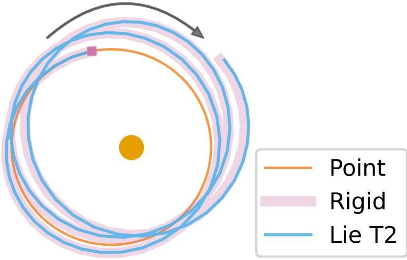
Figure 1: One planet’s orbit around a star: rigid body correction results in a precession, i.e. slow rotation of the orbital axis. Our method, ‘Lie T2’, learns $V$ from data and predicts a trajectory that matches the ground truth with the rigid body potential.

Deep Neural Networks (DNN) have been demonstrated to be effective tools for learning dynamical systems from data. One important class of systems to be learned have dynamics described by physical laws, whose structure can be exploited by learning the Hamiltonian of the system instead of the vector field [1, 2]. An appropriately learned Hamiltonian can endow the learned system with properties such as superior long prediction accuracy [3] and applicability to chaotic systems [4, 3, 5].

To learn continuous dynamics from discrete data, one important step is to bridge the continuous and discrete times. Seminal work initially approximated the time derivative via finite differences and then matched it with a learned (Hamiltonian) vector field[1, 2]. Recent efforts avoid the inaccuracy of finite difference by numerically integrating the learned vector field. Especially relevant here is SRNN [6], which uses a symplectic integrator to ensure the learned dynamics is symplectic (a necessity for Hamiltonian systems). Although SRNN only demonstrated learning separable Hamiltonians, breakthrough in symplectic integration of arbitrary Hamiltonians [7] was used to extend SRNN [8]. Further efforts on improving the time integration error have also been made [9, 10, 11]. Meanwhile, alternative approaches based on learning a symplectic map instead of the Hamiltonian also demonstrated efficacy [12, 3], although these approaches have not been extended to non-Euclidean problems.

In fact, one relatively under-explored area is learning Hamiltonian dynamics on manifolds like the Lie group manifold family. One important member of this family is $\mathsf{SO}(n)$, which describes isometries in $\mathbb{R}^{n}$ and is important for, e.g., dynamical astronomy. The evolution of celestial bodies correspond to a mechanical system, and the 2- and 3-body problems have been a staple problem in works on learning Hamiltonian (e.g., [1, 6, 3, 15]); however, the Newtonian (point-mass) gravity considered is already well understood. Practical problems in planetary dynamics are complicated by higher-order physics such as planet spin-orbit interaction, tidal dissipation, and general relativistic correction. While it is unclear what would be a perfect scientific model for these effects, planetary rotation is a necessary component to account for spin-orbit interaction and tidal forcing, creating an $\mathsf{SO}(3)^{\otimes N}$ component of the configuration space. To learn these physics from data, we need to learn on the Lie group.

Rigid body dynamics also play important roles in other applications such as robotics. In a seminal work [16], Hamiltonian dynamics on $\mathsf{SO}(3)$ are used to learn rigid body dynamics for a quadrotor. In that work, Runge-Kutta 4 integrator is used. Consequently, the method is applicable to short time-horizon (see Sec.3 and last paragraph of Sec.2).

For our problem of learning non-Newtonian astronomy, the time-horizon has to be long. Hence, we use a different approach by leveraging a Lie-group preserving symplectic integrator. Structure-preserving integration of dynamical systems on manifolds has been extensively studied in literature, for example for Lie groups [17, 18, 19, 20, 21] and more broadly, geometric integration [22, 23, 24, 25].

In summary, we propose a deep learning methodology for performing data-driven discovery of non-Newtonian astronomy. By leveraging the use of a symplectic Lie-group manifold preserving integrator, we show how a non-Euclidean Hamiltonian can be learned for accurate prediction of non-Newtonian effects. Moreover, we provide insights that show the importance of both symplecticity and exact preservation of the Lie-group manifold in training stability.

2 Method

Given observations of a dynamically evolving system, our goal is to learn the physics that governs its evolution from the data. Denote by $(\mathbf{q}_{k,l},\mathbf{R}_{k,l},\mathbf{p}_{k,l},\mathbf{\Pi}_{k,l})_{k=1}^{K},\;l\in[L]$ a dataset of snapshots of $L$ continuous-time trajectories of a system with $N$ interacting rigid bodies. That is,

$$(\mathbf{q}_{k,l},\mathbf{R}_{k,l},\mathbf{p}_{k,l},\mathbf{\Pi}_{k,l})=\big{(}\mathbf{q}_{l}(k\Delta t),\mathbf{R}_{l}(k\Delta t),\mathbf{p}_{l}(k\Delta t),\mathbf{\Pi}_{l}(k\Delta t)\big{)},$$

where $\mathbf{q}_{l}(t),\mathbf{R}_{l}(t),\mathbf{p}_{l}(t),\mathbf{\Pi}_{l}(t)$ is a solution of some latent Hamiltonian ODE to be learned corresponding to mechanical dynamics on $T^{*}\mathsf{SE(3)}^{\otimes N}$. $\Delta t$ is a (possibly large) observation timestep, $\mathbf{R}\in\mathsf{SO}(3)^{\otimes N}$ is the rotational configuration of the $N$ rigid bodies, and $\mathbf{\Pi}\in\mathfrak{so}(3)^{\otimes N}$ denotes each’s angular momentum in their respective body frames.

Importantly, since the configuration space $\mathcal{Q}=\mathsf{SE(3)}^{\otimes N}$ is not flat, the mechanical dynamics are not given by $\dot{\mathcalboondox{q}}=\partialderivative{\mathcal{H}}{\mathcalboondox{p}},\dot{\mathcalboondox{p}}=-\partialderivative{\mathcal{H}}{\mathcalboondox{q}}$ for some Hamiltonian $\mathcal{H}$ that depends on the generalized coordinates $\mathcalboondox{q}\in\mathcal{Q}$ and generalized momentum $\mathcalboondox{p}\in T^{*}{q}\mathcal{Q}$. Instead, the equations of motion can be derived via either Lagrange multipliers [20, 26] or a Lie group variational principle [20, 27], which will be

assuming a physical Hamiltonian $\mathcal{H}(\mathbf{q},\mathbf{R},\mathbf{p},\mathbf{\Pi})=\sum_{i=1}^{N}\frac{1}{2}\mathbf{p}_{i}^{T}\mathbf{p}_{i}/m_{i}+\sum_{i}\frac{1}{2}\mathbf{\Pi}^{T}_{i}\mathbf{J}_{i}^{-1}\mathbf{\Pi}_{i}+V(\mathbf{q},\mathbf{R})$ that sums total (translation and rotational) kinetic energy and interaction potential $V$, where $m_{i},\mathbf{J}_{i}$ denote the mass and inertial tensor of the $i$th body, and $F_{\mathbf{p}},F_{\mathbf{\Pi}}$ are forcing terms to model nonconervative forces. $\mathbf{\Pi}_{i}\in\mathbb{R}^{3}$ is a vector, $\wedge$ is the map from $\mathbb{R}^{3}$ to $\textrm{Skew}_{3}$ and $\vee$ is its inverse ([20] for more details). By learning the potential $V$, external forcing $F_{\mathbf{p}}$ and torque $F_{\mathbf{\Pi}}$, we can learn the physics of the system.

2.1 Machine Learning Challenges Posed by Dynamical Astronomy

We study this setup because it helps answer scientific questions like: what physics governs the motions of celestial bodies, such as planets in a planetary system? The leading order physics is of course already well known, namely these bodies can be approximated by point masses that are interacting through a $1/r$ gravitational potential. However, planets are not point masses, and their rotations matter because they shape planetary climates [28, 29] and even feedback to their orbits [30]. This already starts to alter $V$ even if one only considers classical gravity. For example, the gravitational potential $V$ for interacting bodies of finite sizes should be $V(\mathbf{q},\mathbf{R})=\sum_{i<j}V_{i,j}$, where

$$V_{i,j}(\mathbf{q},\mathbf{R})=\int_{\mathcal{B}_{i}}\int_{\mathcal{B}_{j}}-\frac{\mathcal{G}\rho(\mathbf{x}_{i})\rho(\mathbf{x}_{j})}{\norm{\mathbf{q}_{i}+\mathbf{R}_{i}\mathbf{x}_{i}-\mathbf{q}_{j}-\mathbf{R}_{j}\mathbf{x}_{j}}}\differential{\mathbf{x}_{i}}\differential{\mathbf{x}_{j}}\;\;\;=\;\;\;\underbrace{-\frac{\mathcal{G}m_{i}m_{j}}{\norm{\mathbf{q}_{i}-\mathbf{q}_{j}}}}_{V_{i,j,\textrm{point}}}+\underbrace{O\left(\frac{1}{\norm{q_{i}-q_{j}}^{2}}\right)}_{V_{i,j,\textrm{resid}}}.$$ (2)

Working with the full potential is complicated since $\mathcal{B}_{i}$ is not known and the integral is not analytically known. Can we directly learn $V_{\textrm{resid}}$ from time-series data?

Classical gravity (i.e. Newtonian physics) is not the only driver of planetary motion — tidal forces and general relativity (GR) matter too. The former provides a dissipation mechanism and plays critical roles in altering planetary orbits [31, 32]; the latter doesn’t need much explanation and has been demonstrated by, e.g., Mercury’s precessing orbit [33]. Tidal forces depend on celestial bodies’ rotations [34] and thus is a function of both $\mathbf{q},\mathbf{R}$. GR’s effects cannot be fully characterized with classical coordinates $\mathbf{q},\mathbf{R},\mathbf{p},\mathbf{\Pi}$, but post-Newtonian approximations based purely on these coordinates are popular [35]. Can we learn both purely from data if we did not have theories for either?

In addition to the scientific questions, there are also significant machine learning challenges:

Multiscale dynamics. Rigid-body correction ($V_{\textrm{resid}}$), tidal force, and GR correction are all much smaller forces compared to point-mass gravity. Consequently, their effects do not manifest until long time. Thus, one challenge for learning them is that the dynamical system exhibits different behaviors over multiple timescales. It is reasonable to require long time series data for the small effects to be learned; meanwhile, when observations are expensive to make, the observation time step $\Delta t$ can be much longer than the smallest timescales. Can we still learn the physics in this case? We will leverage symplectic integrator and its mild growth of error over long time [26, 7] to provide a positive answer.

Respecting the Lie group manifold. However, even having a symplectic integrator is not enough because the position variable of the latent dynamics (i.e. truth) stays on $\mathsf{SE(3)}^{\otimes N}$. If the integrated solution falls off this manifold such that $\mathbf{R}^{\intercal}\mathbf{R}=I$ no longer holds, it is not only incorrect but likely misleading for the learning of $V(\mathbf{q},\mathbf{R})$. Popular integrators such as forward Euler, Runge-Kutta 4 (RK4) and Leapfrog [1, 6, 36] unfortunately do no maintain the manifold structure.

2.2 Learning with Lie Symplectic RNNs

Our method can be viewed as a Lie-group generalization of the seminal work of SRNN [6], where a good integrator that is both symplectic and Lie-group preserving is employed as a recurrent block.

Lie $\mathrm{T}_{2}$: A Symplectic Lie-Group Preserving Integrator. To construct an integrator that achieves both properties, we borrow from [20] the idea of Lie-group and symplecticity preserving splitting, and split our Hamiltonian as $\mathcal{H}=\mathcal{H}_{\textrm{KE}}+\mathcal{H}_{\textrm{PE}}+\mathcal{H}_{\textrm{asym}}$, which contains the axial-symmetric kinetic energy, potential energy and asymmetric kinetic energy correction terms. This enables computing the exact integrators $\phi_{t}^{[\textrm{KE}]},\phi_{t}^{[\textrm{PE}]}$ and $\phi_{t}^{[\textrm{asym}]}$ (see App B for details). We then construct a 2nd-order symplectic integrator Lie $\mathrm{T}_{2}$ by applying the Strang composition scheme. To account for non-conservative forces, the corresponding non-conservative momentum update $\phi^{[\textrm{force}]}:(\mathbf{p},\mathbf{\Pi})\leftarrow F(\mathbf{q},\mathbf{R},\mathbf{p},\mathbf{\Pi})$ is inserted in the middle of the composition [20]. This gives $\phi_{h}^{[\textrm{Lie $\mathrm{T}_{2}$}]}$ for stepsize $h$ as

$$\phi_{h}^{\textrm{Lie $\mathrm{T}_{2}$}}\coloneqq\phi_{h/2}^{[\textrm{KE}]}\,\circ\,\phi_{h/2}^{[\textrm{PE}]}\,\circ\,\phi_{h/2}^{[\textrm{asym}]}\,\circ\,\phi_{h}^{[\textrm{force}]}\,\circ\,\phi_{h/2}^{[\textrm{asym}]}\,\circ\phi_{h/2}^{[\textrm{PE}]}\,\circ\,\phi_{h/2}^{[\textrm{KE}]}$$ (3)

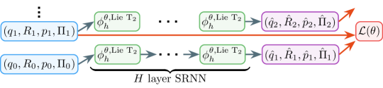
Figure 2: Inputs are fed through a recurrent layer with Lie $\mathrm{T}_{2}$. Prediction error is used as a loss on $\theta$.

A Recurrent Architecture for Nonlinear Regression. Given the simplicity of $V_{\textrm{point}}$, we assume this is known and learn $V_{\textrm{resid}}$ and $F^{\theta}$ with multi-layer perceptron (MLP) $V^{\theta}_{\textrm{resid}}$ and $F^{\theta}$ without assuming any pairwise structure (see App C for discussion). We then use $\phi^{\theta,\textrm{Lie $\mathrm{T}_{2}$}}$ to integrate dynamics forward, where $\theta$ denotes the dependence on the networks. However, when the temporal spacing between observations $\Delta t$ is large, using a single $\phi_{\Delta t}^{\theta,\textrm{Lie $\mathrm{T}_{2}$}{}}$ will result in large errors for the fast timescale dynamics. Instead, we compose $\phi_{h}^{\theta,\textrm{Lie $\mathrm{T}_{2}$}{}}$ $H$ times as $(\hat{\mathcalboondox{q}}_{k+1,l},\hat{\mathcalboondox{p}}_{k+1,l})=\phi_{h}^{\theta,\textrm{Lie $\mathrm{T}_{2}$}}\circ\dots\circ\phi_{h}^{\theta,\textrm{Lie $\mathrm{T}_{2}$}}(\mathcalboondox{q}_{k,l},\mathcalboondox{p}_{k,l})$, where $H=h/\Delta t\in\mathbb{Z}$ determines the integration stepsize $h$. We perform training by minimizing the following empirical loss over random minibatches of size $N_{b}$

$$\mathcal{L}(\theta)\coloneqq\frac{1}{N_{b}\,K}\sum_{l=1}^{N_{b}}\sum_{k=1}^{K}\Big{\{}\norm{\mathcalboondox{q}_{k,l}-\hat{\mathcalboondox{q}}_{k,l}^{\theta}}^{2}_{2}+\norm{\mathcalboondox{p}_{k,l}-\hat{\mathcalboondox{p}}_{k,l}^{\theta}}^{2}_{2}\Big{\}}$$ (4)

Note that we do not assume access to the true derivatives $\dot{\mathcalboondox{q}}_{k,j}$ and $\dot{\mathcalboondox{p}}_{k,j}$ used in the loss function of some works [1, 37, 38]. Our training process in summarized in Fig. 2 (see App C for details).

Benefit. Learning an accurate $V^{\theta},F^{\theta}$ requires accurate numerical simulation which also leads to a trainable model. Without preservation of the manifold structure, training can lead to ‘shortcuts’ outside the manifold that seemingly match the data but completely mislead the learning. Symplecticity also plays a vital role in controlling the long time integration error — under reasonable conditions, a $p$th-order symplectic integrator has linear $\mathcal{O}(\Delta th^{p})$ error bound, whereas a $p$th-order nonsymplectic one has an exponential $\mathcal{O}(e^{C\Delta t}h^{p})$ error bound [26, 7]. While these bounds do not matter for small $\Delta t$, they are significant for multiscale problems where $\Delta t$ is macroscopic but $h$ is microscopic. Consequently, improving error estimates for a nonsymplectic integrator by reducing $h$ makes the RNN exponentially deep — this often renders training difficult [39] and is not desirable.

3 Results

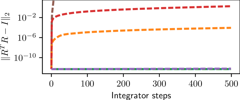
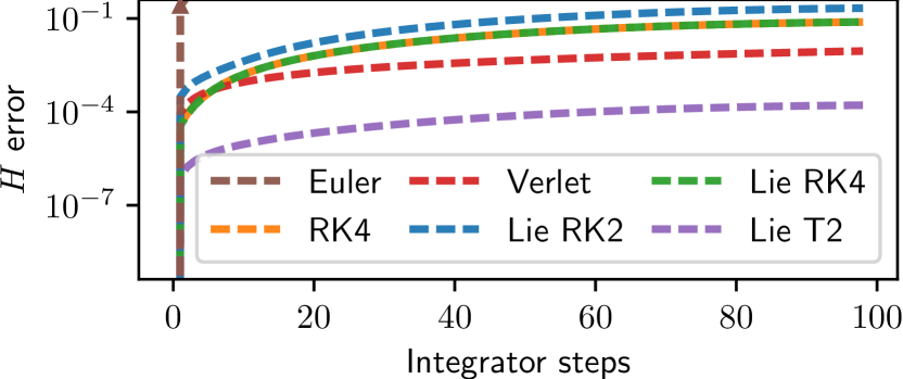
Figure 3: Results on TRAPPIST-1 with short data separation. Top: $SO(3)$ manifold error. Bottom: Hamiltonian error over the integrated trajectory. Only Lie T2 achieves low errors in both metrics.

We aim to answer two questions. Q1 Can we learn multiscale physics? Q2 How important are symplecticity (${\color[rgb]{0,0,0}\bm{\mathcal{S}}}$) and Lie-group preservation (${\color[rgb]{0,0,0}\bm{\mathcal{L}}}$) for learning? The closest baseline for our problem is work of [16], which learns short timescale rigid-body Hamiltonian dynamics for robotics. Placed in our framework, their work corresponds to using RK4 for the recurrent block, which is neither ${\color[rgb]{0,0,0}\bm{\mathcal{S}}}$ nor ${\color[rgb]{0,0,0}\bm{\mathcal{L}}}$. Therefore, to investigate Q2, we vary the choice of integrator in our framework as follows: Normal: Explicit Euler, RK4. ${\color[rgb]{0,0,0}\bm{\mathcal{S}}}$: Verlet. ${\color[rgb]{0,0,0}\bm{\mathcal{L}}}$: Lie RK2(CF2) and Lie RK4(CF4) [21]. We leave the precise details to Apps C and D.

Toy Two-Body Problem. We consider an illustrative two-body problem to demonstrate the effects of $V_{\textrm{rigid}}$. In Fig. 1 ‘Point’ & ‘Rigid’ denote exact solutions for a point-mass and rigid-body potential, and ‘Lie T2’ the prediction of our method based on a $V$ learned from data. Compared to ‘Point’, ‘Rigid’ induces an apsidal precession (rotation of the orbital axis) due to spin-orbit couplings. Our method successfully predict this interaction and matches the trajectory of ‘Rigid’.

We next test our method by learning the dynamics of the TRAPPIST-1 system [40] which consists of seven earth-sized planets and is notable for potential habitability for terrestrial forms of lives.

TRAPPIST-1, Large $\Delta t$. To answer Q1, we choose a large data timestep $\Delta t=$2.410-3\text{\,}\mathrm{yr}$$. The closest planet has an orbital period of $\sim 2\Delta t$ ($4.110-3\text{\,}\mathrm{yr}$), while the rigid body correction, tidal force and GR correction act on much longer scales. Only Lie $\mathrm{T}_{2}$ successfully trains. All other methods diverge during training (denoted by $\infty$) despite attempts at stabilization with techniques such as normalization (LayerNorm [41], GroupNorm [42]). Reducing $h$ improves integration accuracy, but increases the RNN depth and makes training more unstable. We compare with the solution for point-mass potential only (No Correction). Our method reduces the error up to two orders of magnitude in measures of trajectory error and potential gradients (Table 2). See App E for column definitions.

Table 1: TRAPPIST-1 with long data separation evaluated after $500$ integrator steps. All methods except for Lie $\mathrm{T}_{2}$ diverge during training. $\norm{\Delta q}_{2}$ $\norm{\Delta R}$ $\norm{\Delta\dot{p}}_{2}$ $\norm*{\Delta\dot{\Pi}}_{2}$ No Corrections $8.610-06$ $1.610+00$ $3.310+00$ $4.710-02$ Euler, RK4, Verlet, Lie RK2, Lie RK4 $\infty$ $\infty$ $\infty$ $\infty$ Lie $\bm{\mathrm{T}_{2}}$ (Ours) $6.110-08$ $4.010-02$ $1.210-01$ $3.110-03$ Table 2: TRAPPIST-1 with short data separation evaluated after $500$ integrator steps. $\norm{\Delta q}_{2}$ $\norm{\Delta R}$ $\norm*{\Delta\partialderivative{V}{\mathbf{q}}}_{2}$ $\norm*{\Delta\partialderivative{V}{\mathbf{R}}}_{2}$     Euler $\infty$ $\infty$ $\infty$ $\infty$     RK4 $1.610-05$ $3.910-01$ $1.510+03$ $7.910-01$ ${\color[rgb]{0,0,0}\bm{\mathcal{S}}}{}\phantom{{\color[rgb]{0,0,0}\bm{\mathcal{L}}}{}}$Verlet $8.610-08$ $2.010+07$ $1.610+01$ $4.110-01$ $\phantom{{\color[rgb]{0,0,0}\bm{\mathcal{S}}}{}}{\color[rgb]{0,0,0}\bm{\mathcal{L}}}$Lie RK2 $5.310-05$ $3.310-01$ $2.610+02$ $7.610-01$ $\phantom{{\color[rgb]{0,0,0}\bm{\mathcal{S}}}{}}{\color[rgb]{0,0,0}\bm{\mathcal{L}}}$Lie RK4 $1.610-05$ $3.510-01$ $1.510+03$ $8.410-01$ ${\color[rgb]{0,0,0}\bm{\mathcal{S}}}{}{\color[rgb]{0,0,0}\bm{\mathcal{L}}}$Lie $\mathrm{T}_{2}$ (Ours) $8.010-08$ $2.410-01$ $1.610+01$ $4.010-01$

TRAPPIST-1, Small $\Delta t$. To gain more insight on Q2, we shrink $\Delta t$ until almost all methods can converge and only consider conservative forces (i.e. no tidal force or GR). The mean errors in the predicted trajectory and derivatives of the learned potential $V$ after $500$ integrator steps are shown in Table 2. Both ${\color[rgb]{0,0,0}\bm{\mathcal{S}}}$ methods achieve small errors in position related terms. Verlet has a large rotational error since it does not integrate on the rotation manifold. ${\color[rgb]{0,0,0}\bm{\mathcal{L}}}$ methods achieve lower rotational errors but are worse elsewhere. Lie $\mathrm{T}_{2}$ being both ${\color[rgb]{0,0,0}\bm{\mathcal{S}}}{}{\color[rgb]{0,0,0}\bm{\mathcal{L}}}{}$ achieves the lowest error on both fronts.

4 Broader Impact

Our work presents an approach for learning multiscale, higher order physics on the Lie-group manifold in the context of non-Newtonian astronomy. This research, though directly applicable to astronomy, can also be applied to perform data-driven discovery multiscale phenomena on Lie groups in other fields.

Appendix A Rigid Body Equations of Motion

We present two derivations from Chen et al. [20]. The first derivation derives a constrained Hamiltonian system via Lagrange multipliers, while the second uses a variational principle for mechanics on Lie groups. We also note that the same equations can be derived via the use of the Port-Hamiltonian framework as in Duong and Atanasov [16], though they choose to express the linear momentum coordinates in the moving body frame rather than the inertial frame as is done in this work.

A.1 Constrained Hamiltonian System

Since the manifold $\mathsf{SE}(3)^{\otimes N}$ is a product space of the individual manifolds $\mathsf{SE}(3)$, we consider the latter for brevity and drop indices $i$ for each body. Furthermore, $\mathsf{SE}(3)$ can be seen as the product space of $\mathbb{R}^{3}\times\mathsf{SO}(3)$ for which the former is unconstrained, so we focus our attention on the latter. We can view $\mathbf{R}$ to be in the embedded Euclidean space $\mathbf{R}^{3\times 3}\xhookleftarrow{}\mathsf{SO}(3)$ and use $\mathbf{R}\in\mathsf{SO}(3)\coloneqq h(\mathbf{R})=\{\mathbf{R}^{\intercal}\mathbf{R}-\mathbf{I}_{3\times 3}=\mathbf{0}_{3\times 3}\}$ as a holonomic constraint. Using Lagrange multipliers $\mathbf{\Lambda}$ [26] for the constraint $h$ gives us the following Lagrangian

$$L(\mathbf{R},\dot{\mathbf{R}})=\frac{1}{2}\Tr\left[\dot{\mathbf{R}}\mathbf{J}_{d}{}\dot{\mathbf{R}}\right]-V(\mathbf{R})-\frac{1}{2}\Tr\left[\mathbf{\Lambda}^{\intercal}(\mathbf{R}^{\intercal}\mathbf{R}-\mathbf{I}_{3\times 3})\right]$$ (A5)

where $\mathbf{J}_{d}{}$ denotes the nonstandard moment of inertia [20, 27]

$$\mathbf{J}_{d}\coloneqq\int_{\mathcal{B}}\rho(\mathbf{x})\mathbf{x}\mathbf{x}^{\intercal}\differential{\mathbf{x}},\qquad\mathbf{J}_{d}=\Tr[\mathbf{J}]\mathbf{I}_{3\times 3}-\mathbf{J},\qquad\mathbf{J}=\Tr[\mathbf{J}_{d}]\mathbf{I}_{3\times 3}-\mathbf{J}_{d},$$ (A6)

and

$$\mathbf{\Lambda}=\begin{bmatrix}\lambda_{1}&\lambda_{4}&\lambda_{6}\\ \lambda_{4}&\lambda_{2}&\lambda_{5}\\ \lambda_{6}&\lambda_{5}&\lambda_{3}\end{bmatrix}\in\mathbb{R}^{3\times 3}$$ (A7)

is a 6-dimensional symmetric matrix of Lagrange multipliers. Performing the Legendre transform for (A5) gives us the conjugate rotational momentum $\mathbf{P}$ as

$$\mathbf{P}=\partialderivative{L(\mathbf{R},\dot{\mathbf{R}})}{\dot{\mathbf{R}}}=\dot{\mathbf{R}}\mathbf{J}_{d}$$ (A8)

and corresponding Hamiltonian

$$H(\mathbf{R},\mathbf{P})=\frac{1}{2}\Tr\left[\mathbf{P}{}\mathbf{J}_{d}{}^{-1}\mathbf{P}{}\right]+V(\mathbf{R})+\frac{1}{2}\Tr\left[\mathbf{\Lambda}^{\intercal}(\mathbf{R}^{\intercal}\mathbf{R}-\mathbf{I}_{3\times 3})\right]$$ (A9)

The constraint for $\mathbf{P}$ can be obtained by taking the time derivative of $h(\mathbf{R})=0$ according to Haier et al. [22], i.e., $\mathbf{J}_{d}^{-1}\mathbf{P}^{\intercal}\mathbf{R}+\mathbf{R}^{\intercal}\mathbf{P}\mathbf{J}_{d}^{1}=\mathbf{0}_{3\times 3}$. Hence, our equations of motion so far looks like

$$\begin{dcases}\dot{\mathbf{R}}=\partialderivative{H}{\mathbf{P}}=\mathbf{P}\mathbf{J}_{d}^{-1}\\ \dot{\mathbf{P}}=-\partialderivative{H}{\mathbf{R}}=-\partialderivative{V}{\mathbf{R}}-\mathbf{R}\mathbf{\Lambda}\end{dcases}$$ (A10)

on the manifold

$$\mathcal{M}\coloneqq\{(\mathbf{R},\mathbf{P})|\mathbf{R}^{\intercal}\mathbf{R}=\mathbf{I}_{3\times 3},\quad\mathbf{J}_{d}^{-1}\mathbf{P}^{\intercal}\mathbf{R}+\mathbf{R}^{\intercal}\mathbf{P}\mathbf{J}_{d}^{-1}=\mathbf{0}_{3\times 3}$$ (A11)

Let $\hat{\mathbf{\Omega}}=\mathbf{R}^{\intercal}\dot{\mathbf{R}}$ denote the body’s angular velocity in the inertial frame, where $\wedge$ denotes the cross-product operation $\hat{u}v=u\times v$. Then, it can written using $P$ as

$$\hat{\mathbf{\Omega}}=\mathbf{R}^{\intercal}\mathbf{P}\mathbf{J}_{d}^{-1}$$ (A12)

Taking the time derivative of $\hat{\mathbf{\Omega}}$ gives

$$\dot{\hat{\mathbf{\Omega}}}=\mathbf{J}_{d}^{-1}\mathbf{P}^{\intercal}\mathbf{P}\mathbf{J}_{d}^{-1}+\mathbf{R}^{\intercal}\left(-\partialderivative{V(\mathbf{R})}{\mathbf{R}}-\mathbf{R}\mathbf{\Lambda}\right)\mathbf{J}_{d}^{-1}$$ (A13)

Since our goal is to represent the dynamics of $\mathbf{\Pi}$, we convert the above to the body frame momentum using $\mathbf{\Pi}=\mathbf{J}\mathbf{\Omega}$. Using properties of the hat map [20, Appendix A.1] gives us

$$\hat{\mathbf{\Pi}}=\hat{\mathbf{J}\mathbf{\Omega}}=\Tr[\mathbf{J}_{d}]\hat{\mathbf{\Omega}}-\widehat{\mathbf{J}_{d}\mathbf{\Omega}}=\hat{\mathbf{\Omega}}\mathbf{J}_{d}{}-\mathbf{J}_{d}{}\hat{\mathbf{\Omega}}^{\intercal}.$$ (A14)

Taking the time derivative of the above then gives

$$\dot{\hat{\mathbf{\Pi}}} =\dot{\hat{\mathbf{\Omega}}}\mathbf{J}_{d}{}-\mathbf{J}_{d}{}\dot{\hat{\mathbf{\Omega}}},$$ (A15)

$$=\left(\mathbf{J}_{d}^{-1}\mathbf{P}^{\intercal}\mathbf{P}-\mathbf{P}^{\intercal}\mathbf{P}\mathbf{J}_{d}^{-1}\right)-\left(\mathbf{R}^{\intercal}\partialderivative{V(\mathbf{R})}{\mathbf{R}}+\left(\partialderivative{V(\mathbf{R})}{\mathbf{R}}\right)^{\intercal}\mathbf{R}\right)-\left(\mathbf{\Lambda}-\mathbf{\Lambda}^{\intercal}\right),$$ (A16)

$$=\left(\mathbf{J}_{d}^{-1}\mathbf{P}^{\intercal}\mathbf{P}-\mathbf{P}^{\intercal}\mathbf{P}\mathbf{J}_{d}^{-1}\right)-\left(\mathbf{R}^{\intercal}\partialderivative{V(\mathbf{R})}{\mathbf{R}}+\left(\partialderivative{V(\mathbf{R})}{\mathbf{R}}\right)^{\intercal}\mathbf{R}\right),$$ (A17)

where the symmetric $\mathbf{\Lambda}$ vanishes on the last line.

Since $\mathbf{P}=\mathbf{R}\hat{\mathbf{\Omega}}\mathbf{J}_{d}{}$, applying properties of the hat map [20, Appendix A.1] further simplifies the above as

$$\hat{\dot{\mathbf{\Pi}}} =\left(\hat{\mathbf{\Omega}}^{\intercal}\hat{\mathbf{\Omega}}\mathbf{J}_{d}{}-\mathbf{J}_{d}{}\hat{\mathbf{\Omega}}^{\intercal}\hat{\mathbf{\Omega}}\right)-\left(\mathbf{R}^{\intercal}\partialderivative{V(\mathbf{R})}{\mathbf{R}}+\left(\partialderivative{V(\mathbf{R})}{\mathbf{R}}\right)^{\intercal}\mathbf{R}\right),$$ (A18)

$$=\widehat{\mathbf{\Omega}\times\mathbf{J}_{d}{}\mathbf{\Omega}}-\left(\mathbf{R}^{\intercal}\partialderivative{V(\mathbf{R})}{\mathbf{R}}+\left(\partialderivative{V(\mathbf{R})}{\mathbf{R}}\right)^{\intercal}\mathbf{R}\right).$$ (A19)

Thus, applying the vee map and converting back to $\mathbf{J}$ and $\mathbf{\Pi}$ gives

$$\dot{\mathbf{\Pi}} =\mathbf{\Omega}\times\mathbf{J}_{d}{}\mathbf{\Omega}-\left(\mathbf{R}^{\intercal}\partialderivative{V(\mathbf{R})}{\mathbf{R}}+\left(\partialderivative{V(\mathbf{R})}{\mathbf{R}}\right)^{\intercal}\mathbf{R}\right)^{\vee},$$ (A20)

$$=\mathbf{\Omega}\times()\Tr[\mathbf{J}]-\mathbf{J})\mathbf{\Omega}-\left(\mathbf{R}^{\intercal}\partialderivative{V(\mathbf{R})}{\mathbf{R}}+\left(\partialderivative{V(\mathbf{R})}{\mathbf{R}}\right)^{\intercal}\mathbf{R}\right)^{\vee},$$ (A21)

$$=-\mathbf{\Omega}\times\mathbf{J}\mathbf{\Omega}-\left(\mathbf{R}^{\intercal}\partialderivative{V(\mathbf{R})}{\mathbf{R}}+\left(\partialderivative{V(\mathbf{R})}{\mathbf{R}}\right)^{\intercal}\mathbf{R}\right)^{\vee},$$ (A22)

$$=\mathbf{\Pi}\times\mathbf{J}^{-1}\mathbf{\Pi}-\left(\mathbf{R}^{\intercal}\partialderivative{V(\mathbf{R})}{\mathbf{R}}+\left(\partialderivative{V(\mathbf{R})}{\mathbf{R}}\right)^{\intercal}\mathbf{R}\right)^{\vee}.$$ (A23)

Hence, the rotational equations of motion on $\mathsf{SO}(3)$ are

$$\begin{dcases}\dot{\mathbf{R}}=\mathbf{R}\widehat{\mathbf{J}^{1}\mathbf{\Pi}},\\ \dot{\mathbf{\Pi}}=\mathbf{\Pi}\times\mathbf{J}^{-1}\mathbf{\Pi}-\left(\mathbf{R}^{\intercal}\partialderivative{V(\mathbf{R})}{\mathbf{R}}-\left(\partialderivative{V(\mathbf{R})}{\mathbf{R}}\right)^{\intercal}\mathbf{R}\right)^{\vee}.\end{dcases}$$ (A24)

A.2 Variational Principle for Mechanics on the Lie Group

We can also apply the Euler-Lagrange equations for Hamilton’s variational principle on a Lie group, a topic that has been well studied (e.g., Marsden and Ratiu [43], Holm et al. [44]) [20], and we summarize the results for the special case of rigid bodies from the expository part of Lee et al. [27].

Denote the infinitesimally varied rotation by $\mathbf{R}_{\epsilon}=\mathbf{R}\exp(\epsilon\hat{\mathbf{\eta}})$, with $\epsilon\in\mathbb{R}$ and $\mathbf{\eta}\in\mathbb{R}^{3}$, where $\exp(\cdot)$ is the exponential map from $\mathfrak{so}(3)$ to $\mathsf{SO}(3)$. The varied angular velocity $\hat{\mathbf{\Omega}}_{\epsilon}$ is

$$\hat{\mathbf{\Omega}}_{\epsilon} =\mathbf{R}_{\epsilon}^{\intercal}\dot{\mathbf{R}}_{\epsilon}=\exp(-\epsilon\hat{\mathbf{\eta}})\left(\dot{\mathbf{R}}\exp(\epsilon\hat{\mathbf{\eta}})+\mathbf{R}\exp(\epsilon\hat{\mathbf{\eta}})\epsilon\hat{\mathbf{\eta}}\right),$$ (A25)

$$=\exp(-\epsilon\hat{\mathbf{\eta}})\hat{\mathbf{\Omega}}\exp(-\epsilon\hat{\mathbf{\eta}})+\exp(-\epsilon\hat{\mathbf{\eta}})\hat{\dot{\mathbf{\eta}}},$$ (A26)

$$=\hat{\mathbf{\Omega}}+\epsilon\left(\hat{\dot{\mathbf{\eta}}}+\hat{\mathbf{\Omega}}\hat{\mathbf{\eta}}-\hat{\mathbf{\eta}}\hat{\mathbf{\Omega}}\right)+O(\epsilon^{2}).$$ (A27)

Consider the action

$$S(\mathbf{\Omega},\mathbf{R})=\int_{t_{0}}^{t_{1}}L(\mathbf{\Omega},\mathbf{R})\differential{t}=\int_{t_{0}}^{t_{1}}\frac{1}{2}\Tr[\hat{\mathbf{\Omega}}\mathbf{J}_{d}{}\hat{\mathbf{\Omega}}]-V(\mathbf{R})\differential{t}.$$ (A28)

Taking the variation $S_{\epsilon}$ of the action $S$, we have

$$\begin{split}S_{\epsilon}(\mathbf{\Omega},\mathbf{R})&=S(\mathbf{\Omega}_{\epsilon},\mathbf{R}_{\epsilon}),\\ &=S(\mathbf{\Omega},\mathbf{R})+\epsilon\int_{t_{0}}^{t_{1}}\bigg{\{}\frac{1}{2}\Tr[-\hat{\dot{\mathbf{\eta}}}\left(\mathbf{J}_{d}{}\hat{\mathbf{\Omega}}+\hat{\mathbf{\Omega}}\mathbf{J}_{d}{}\right)\\ \hfil&\quad+\hat{\mathbf{\eta}}\hat{\mathbf{\Omega}}\left(\mathbf{J}_{d}{}\hat{\mathbf{\Omega}}+\hat{\mathbf{\Omega}}\mathbf{J}_{d}{}\right)-\hat{\mathbf{\eta}}\left(\mathbf{J}_{d}{}\hat{\mathbf{\Omega}}+\hat{\mathbf{\Omega}}\mathbf{J}_{d}{}\hat{\mathbf{\Omega}}\right)\Big{]}+\Tr[\hat{\mathbf{\eta}}\mathbf{R}^{\intercal}\partialderivative{V(\mathbf{R})}{\mathbf{R}}]\bigg{\}}\differential{t}\\ &\quad+O(\epsilon^{2}).\end{split}$$ (A29)

Using Hamilton’s Principle, we have $\evaluated{\derivative{\epsilon}}_{\epsilon=0}S_{\epsilon}=0$, i.e.,

$$\frac{1}{2}\int_{t_{0}}^{t_{1}}\Tr\left[\hat{\mathbf{\eta}}\left\{\widehat{\mathbf{J}\dot{\mathbf{\Omega}}}+\widehat{\mathbf{\Omega}\times\mathbf{J}\mathbf{\Omega}}+2\mathbf{R}^{\intercal}\partialderivative{V(\mathbf{R})}{\mathbf{R}}\right\}\right]\differential{t}=0,$$ (A30)

for any $\mathbf{\eta}\in\mathbb{R}^{3}$. Hence, $\widehat{\mathbf{J}\dot{\mathbf{\Omega}}}+\widehat{\mathbf{\Omega}\times\mathbf{J}\mathbf{\Omega}}+2\mathbf{R}^{\intercal}\partialderivative{V(\mathbf{R})}{\mathbf{R}}$ must be skew-symmetric, giving us

$$\widehat{\mathbf{J}\dot{\mathbf{\Omega}}}=-\widehat{\mathbf{\Omega}\times\mathbf{J}\mathbf{\Omega}}+\left(\partialderivative{V(\mathbf{R})}{\mathbf{R}}^{\intercal}\mathbf{R}-\mathbf{R}^{\intercal}\partialderivative{V(\mathbf{R})}{\mathbf{R}}\right).$$ (A31)

Thus, by definition of $\mathbf{\Pi}$ and applying the vee map, we recover the same update

$$\dot{\mathbf{\Pi}}=\mathbf{\Pi}\times\mathbf{J}^{-1}\mathbf{\Pi}+\left(\partialderivative{V(\mathbf{R})}{\mathbf{R}}^{\intercal}\mathbf{R}-\mathbf{R}^{\intercal}\partialderivative{V(\mathbf{R})}{\mathbf{R}}\right)^{\vee}.$$ (A32)

Appendix B Details of the Lie $\mathrm{T}_{2}$ splitting integrator

The full Hamiltonian $H$ takes the form

$$\mathcal{H}(\mathbf{q},\mathbf{R},\mathbf{p},\mathbf{\Pi})=\sum_{i=1}^{N}\frac{1}{2}\mathbf{p}_{i}^{\intercal}\mathbf{p}_{i}/m_{i}+\frac{1}{2}\mathbf{\Pi}_{i}^{\intercal}\mathbf{J}_{i}^{-1}\mathbf{\Pi}_{i}+V(\mathbf{q},\mathbf{R})$$ (B33)

We borrow from Chen et al. [20] the idea of Lie-group and symplecticity preserving splitting and split our Hamiltonian as $\mathcal{H}=\mathcal{H}_{\textrm{KE}}+\mathcal{H}_{\textrm{PE}}+\mathcal{H}_{\textrm{asym}}$, where

$$\mathcal{H}_{\textrm{KE}} \coloneqq\sum_{i=1}^{N}\frac{1}{2}\mathbf{p}_{i}^{\intercal}\mathbf{p}_{i}/m_{i}+\frac{1}{2}\mathbf{\Pi}_{i}^{\intercal}\mathbf{J}_{i,\text{sym}}^{-1}\mathbf{\Pi}_{i}$$ (B34)

$$\mathcal{H}_{\textrm{PE}} \coloneqq V(\mathbf{q},\mathbf{R})$$ (B35)

$$\mathcal{H}_{\textrm{asym}} \coloneqq\sum_{i=1}^{N}\frac{1}{2}\mathbf{\Pi}_{i}^{\intercal}\mathbf{J}_{i,\textrm{asym}}^{-1}\mathbf{\Pi}_{i}$$ (B36)

where we assume that $\mathbf{J}_{i}$ is axis-symmetric, i.e.,

$$\mathbf{J}_{i}\coloneqq\begin{bmatrix}J_{i}^{(1)}&0&0\\ 0&J_{i}^{(2)}&0\\ 0&0&J_{i}^{(3)}\end{bmatrix}$$ (B37)

and $\mathbf{J}_{i,\text{sym}}^{-1}$ and $\mathbf{J}_{i,\textrm{asym}}^{-1}$ denote the axial-symmetric and residual terms of $\mathbf{J}_{i}^{-1}$ such that $\mathbf{J}_{i,\text{sym}}^{-1}+\mathbf{J}_{i,\textrm{asym}}^{-1}=\mathbf{J}_{i}^{-1}$, i.e.,

$$\mathbf{J}_{i,\text{sym}}^{-1}\coloneqq\begin{bmatrix}1/J_{i}^{(1)}&0&0\\ 0&1/J_{i}^{(1)}&0\\ 0&0&1/J_{i}^{(3)}\end{bmatrix},\qquad\mathbf{J}_{i,\text{asym}}^{-1}\coloneqq\begin{bmatrix}0&0&0\\ 0&1/J_{i}^{(2)}-1/J_{i}^{(1)}&0\\ 0&0&0\end{bmatrix}.$$ (B38)

Then, each of $\mathcal{H}_{\textrm{KE}}+\mathcal{H}_{\textrm{PE}}+\mathcal{H}_{\textrm{asym}}$ can be integrated exactly.

Exact integration of $\bm{\mathcal{H}_{\textrm{KE}}}$

For $\mathcal{H}_{\textrm{KE}}$, we have the equations of motion (using (1a)-(1d) but with $V=0$)

$$\dot{\mathbf{q}}_{i} =\mathbf{p}_{i}/m_{i}$$ (B39a)

$$\dot{\mathbf{p}}_{i} =0$$ (B39b)

$$\dot{\mathbf{R}}_{i} =\mathbf{R}{}_{i}\widehat{\mathbf{J}_{i,\text{sym}}^{-1}\mathbf{\Pi}_{i}}$$ (B39c)

$$\dot{\mathbf{\Pi}}_{i} =\mathbf{\Pi}{}_{i}\times\mathbf{J}_{i,\text{sym}}^{-1}\mathbf{\Pi}_{i}$$ (B39d)

The equation for $\dot{\mathbf{\Pi}}_{i}$ (B39d) is the Euler equation for a free rigid body [20]. It is exactly solvable with a simple expression for axial-symmetric bodies, since in this case $\dot{\mathbf{\Pi}}$ simplifies as

$$\dot{\mathbf{\Pi}}_{i}=\mathbf{\Pi}_{i}\times\mathbf{J}_{i,\textrm{sym}}^{-1}\mathbf{\Pi}_{i}=\begin{bmatrix}\left(1/J_{i}^{(3)}-1/J_{i}^{(1)}\right)\Pi_{i,y}\Pi_{i,z}\\ -\left(1/J_{i}^{(3)}-1/J_{i}^{(1)}\right)\Pi_{i,y}\Pi_{i,z}\\ 0\end{bmatrix}$$ (B40)

Consequently, $\Pi_{i,z}(t)=\Pi_{i,z}(0)$, meaning that we can express the above as the linear differential equation

$$\dot{\mathbf{\Pi}}_{i}(t) =\begin{bmatrix}0&\left(1/J_{i}^{(3)}-1/J_{i}^{(1)}\right)\Pi_{i,z}(0)&0\\ -\left(1/J_{i}^{(3)}-1/J_{i}^{(1)}\right)\Pi_{i,z}(0)&0&0\\ 0&0&0\end{bmatrix}\mathbf{\Pi}_{i}(0)$$ (B41)

$$=-\theta t\widehat{\begin{bmatrix}0\\ 0\\ 1\end{bmatrix}}\mathbf{\Pi}_{i}(0)$$ (B42)

where $\theta\coloneqq\left(1/J_{i}^{(3)}-1/J_{i}^{(1)}\right)\Pi_{i,z}(0)$ and has the solution

$$\mathbf{\Pi}_{i}(t)=\exp\left(-\theta t\widehat{\begin{bmatrix}0\\ 0\\ 1\end{bmatrix}}\right)\mathbf{\Pi}_{i}(0)=R_{z}^{\intercal}(\theta t)\mathbf{\Pi}_{i}(0)$$ (B43)

where $R_{z}$ denotes the rotation matrix around the $z$ axis. Taking the above back to (B39c) then gives us the solution for $\mathbf{R}_{i}$ as well, giving the flow $\phi_{h}^{[\textrm{KE}]}$ of $\mathcal{H}_{\textrm{KE}}$ as

$$\begin{dcases}\mathbf{q}_{i}(h)=\mathbf{q}_{i}(0)+\mathbf{p}_{i}/m_{i}h,\\ \mathbf{p}_{i}(h)=\mathbf{p}_{i}(0),\\ \mathbf{R}_{i}(h)=\mathbf{R}_{i}(0)R_{\mathbf{\Pi}_{i}(0)}\left(\norm{\mathbf{\Pi}_{i}(0)}h/J_{i}^{(1)}\right)R_{z}(\theta h),\\ \mathbf{\Pi}_{i}(h)=R^{\intercal}_{z}(\theta h)\mathbf{\Pi}_{i}(0).\end{dcases}$$ (B44)

Exact integration of $\bm{\mathcal{H}_{\textrm{PE}}}$

For $\mathcal{H}_{\textrm{PE}}$, the equations of motion are [20]

$$\begin{dcases}\dot{\mathbf{q}}_{i}=0,\dot{\mathbf{p}}_{i}=-\partialderivative{V}{\mathbf{q}_{i}},\\ \dot{\mathbf{R}}_{i}=0,\dot{\mathbf{\Pi}}_{i}=-\left(\mathbf{R}_{i}^{\intercal}\partialderivative{V}{\mathbf{R}_{i}}-\left(\partialderivative{V}{\mathbf{R}_{i}}\right)^{\intercal}\mathbf{R}_{i}\right)^{\vee}.\end{dcases}$$ (B45)

Since $\mathbf{q}_{i}$ and $\mathbf{p}_{i}$ stay constant, $\mathbf{p}_{i}$ and $\mathbf{\Pi}_{i}$ change at constant rates. Hence, the flow $\phi_{h}^{[\textrm{PE}]}$ of $\mathcal{H}_{\textrm{PE}}$ is given by

$$\begin{dcases}\mathbf{q}_{i}(h)=\mathbf{q}_{i}(0)\\ \mathbf{p}_{i}(h)=\mathbf{p}_{i}(0)-\partialderivative{V}{\mathbf{q}_{i}}h,\\ \mathbf{R}_{i}(h)=\mathbf{R}_{i}(0),\\ \mathbf{\Pi}_{i}(h)=\mathbf{\Pi}_{i}(0)-\left(\mathbf{R}_{i}^{\intercal}\partialderivative{V}{\mathbf{R}_{i}}-\left(\partialderivative{V}{\mathbf{R}_{i}}\right)^{\intercal}\mathbf{R}_{i}\right)^{\vee}h.\end{dcases}$$ (B46)

Exact integration of $\bm{\mathcal{H}_{\textrm{asym}}}$

Finally, the equations of motion of $\mathcal{H}_{\textrm{asym}}$ are given by (again adapting (1a)-(1d))

$$\begin{dcases}\dot{\mathbf{q}}_{i}=0,\dot{\mathbf{p}}_{i}=0,\\ \dot{\mathbf{R}}_{i}=\mathbf{R}_{i}\widehat{\mathbf{J}_{i,\textrm{asym}}^{-1}\mathbf{\Pi}_{i}},\dot{\mathbf{\Pi}}_{i}=\mathbf{\Pi}_{i}\times\mathbf{J}_{i,\textrm{asym}}^{-1}\mathbf{\Pi}_{i}.\end{dcases}$$ (B47)

which can be solved to obtain the flow $\phi_{h}^{[\textrm{asym}]}$ of $\mathcal{H}_{\textrm{asym}}$ as

$$\begin{dcases}\mathbf{q}_{i}(h)=\mathbf{q}_{i}(0)\\ \mathbf{p}_{i}(h)=\mathbf{p}_{i}(0),\\ \mathbf{R}_{i}(h)=R_{y}(\delta\Pi_{i}^{(2)}h)\mathbf{R}_{i}(0),\\ \mathbf{\Pi}_{i}(h)=R_{y}(-\delta\Pi_{i}^{(2)}h)\mathbf{\Pi}_{i}(0).\end{dcases}$$ (B48)

where $\delta\coloneqq 1/J_{i}^{(2)}-1/J_{i}^{(1)}$.

Having obtained analytical solutions for each of the flows $\phi^{[\textrm{KE}]},\phi^{[\textrm{PE}]},\phi^{[\textrm{asym}]}$, we then combine them with the non-conservative momentum update from the non-conservative forcing terms $F_{\mathbf{p}_{i}}$ and $F_{\mathbf{\Pi}_{i}}$ with flow $\phi_{h}^{[\textrm{force}]}$

$$\mathbf{q}_{i}(h)=\mathbf{q}_{i}(0)\\ \mathbf{p}_{i}(h)=\mathbf{p}_{i}(0)+F_{\mathbf{p}_{i}}h,\\ \mathbf{R}_{i}(h)=\mathbf{R}_{i}(0),\\ \mathbf{\Pi}_{i}(h)=\mathbf{\Pi}_{i}(0)+F_{\mathbf{\Pi}_{i}}h.$$ (B49)

Consequently, the full Lie $\mathrm{T}_{2}$ integrator is obtained by applying the Strang composition scheme to obtain

$$\phi_{h}^{\textrm{Lie $\mathrm{T}_{2}$}}\coloneqq\phi_{h/2}^{[\textrm{KE}]}\circ\phi_{h/2}^{[\textrm{PE}]}\circ\phi_{h/2}^{[\textrm{asym}]}\circ\phi_{h}^{[\textrm{force}]}\circ\phi_{h/2}^{[\textrm{asym}]}\circ\phi_{h/2}^{[\textrm{PE}]}\circ\phi_{h/2}^{[\textrm{KE}]}$$ (B50)

Appendix C Training Details

We implement our method using Jax [45] and use the Haiku framework [46] for constructing the deep neural networks. In all our experiments, we use a multilayer perceptron (MLP) with $3$ hidden layers each of size $256$ with the SiLU activation [47] for all networks ($V_{\text{resid}}^{\theta},F^{\theta}_{p},F^{\theta}_{\Pi}$). Each method is run until convergence. Other common training hyperparameters used are summarized in Table 3.

Structure of $V_{\textrm{resid}}^{\theta}$

Note that we do not assume prior knowledge on the pairwise structure of the potential function $V_{\text{resid}}$ or of the forcing terms $F_{\bf{p}},F_{\bf{\Pi}}$. More specifically, since the true Gravitational potential (2) only acts pairwise between rigid bodies, the rigid body correction potential also acts pairwise and has the structure

$$V_{\text{resid}}(\mathbf{q},\mathbf{R})=\sum_{i<j}V_{i,j,\text{resid}}(\mathbf{q}_{i},\mathbf{q}_{j},\mathbf{R}_{i},\mathbf{R}_{j}).$$ (C51)

For the forcing terms, the tidal forcing term also acts pairwise with coupled effects on $\bf{\mathbf{p}}_{i}$ and $\bf{\Pi}_{i}$ due the relationship between forces and torques, while the post-Newton general-relativity correction term acts on each planet individually and affects only $\bf{\mathbf{p}}_{i}$. However, in this work, we assume that none of this prior knowledge is available and aim to learn everything purely from data. Hence, we choose to learn the high dimensional forms of $V_{\text{resid}},F_{\bf{p}},F_{\bf{\Pi}}$. The fact that we were able to obtain improvements despite the high dimensionality of the input space ($8$ planets each with $(\mathbf{q}_{i},\mathbf{R}_{i})\in\mathbb{R}^{3}\times\mathbb{R}^{3\times 3}\approx\mathbb{R}^{12}$, i.e., $\mathbb{R}^{96}$ for $V$ and $\mathbb{R}^{144}$ for $F_{\bf{p}},F_{\bf{\Pi}}$) is an indication of the generality of our approach. We believe that the proposed approach can be made more scalable and have better generalization if we do assume some knowledge about the structure of the forces at play and instead, e.g., learn $V_{\text{resid}}^{\theta}(\mathbf{q}_{i},\mathbf{q}_{j},\mathbf{R}_{i},\mathbf{R}_{j},\phi_{i},\phi_{j})$ instead of the more general $V_{\text{resid}}^{\theta}(\mathbf{q},\mathbf{R})$ and similarly for the forcing terms, where $\phi_{i},\phi_{j}$ contains known or potentially learned information about physical properties about each rigid body which are needed. Here, since the ordering of $i$ and $j$ is not important, some type of permutation-invariant encoding such as [48] should be used to further improve generalization.

Training

All experiments are done on a single RTX 3090 locally. The length of each run is dependent on the complexity of the integrator. For example, explicit Euler is the simplest and has the fastest per-iteration time, while Lie RK4 has the slowest per-iteration time. The Lie T2 integrator has a per-iteration time between the two extremes with each experiment taking approximately three hours.

Table 3: Common hyperparameters used for training in all experiments.

Name	Value
Batch size	$256$
Optimizer	AdamW [49]
Learning Rate	$410-4$

Data generation

We use the GRIT simulator [20] for generating the dataset in all cases. Each dataset consists of $32$ different trajectories, which is then split in a $80$-$20$ training-validation split. Each trajectory is then further subsampled to provide $128$ tuples $(\mathbf{q},\mathbf{R},\mathbf{p},\mathbf{\Pi})$ of datapoints. Each trajectory is generated by adding small multiplicative Gaussian noise to the coordinates of each body.

C.1 Toy Two-Body Problem

The parameters for this system were hand-picked to provide intuition on how the additional corrections differ from the pure point-mass potential that is widely used in other Hamiltonian learning literature.

C.2 TRAPPIST-1

The initial conditions for this system were taken directly from the TRAPPIST-1 example from GRIT.

Appendix D Details on Integrators used for Comparison in Section 3

To answer the question Q2 of how important are symplecticity (${\color[rgb]{0,0,0}\bm{\mathcal{S}}}$) and Lie-group preservation (${\color[rgb]{0,0,0}\bm{\mathcal{L}}}$) for learning, we vary the choice of integrator in our experiments. The integrators used can be broadly split into four categories:

Neither Symplectic ${\color[rgb]{0,0,0}\bm{\mathcal{S}}}$ nor Lie-group preserving ${\color[rgb]{0,0,0}\bm{\mathcal{L}}}$: This category contains the popular explicit Euler and Runge-Kutta 4 integrators, neither of which are symplectic or Lie-group preserving. The finite-difference scheme from Greydanus et al. [1], Greydanus and Sosanya [37] can be interpreted as an application of the explicit Euler integrator David and Méhats [10]. Explicit Euler is also used in the works of . Runge-Kutta 4 is a popular fourth-order integrator due to its implementation simplicity and is used in Finzi et al. [13], Zhong et al. [50, 51, 14], Duong and Atanasov [16].

Symplectic ${\color[rgb]{0,0,0}\bm{\mathcal{S}}}$ but not Lie-group preserving ${\color[rgb]{0,0,0}\bm{\mathcal{L}}}$: This category contains the verlet integrator, which we define loosely in the current work as the integrator obtained by using classical splitting and Strang composition, but without performing exact integration on the manifold. In the Euclidean case where $\mathcal{H}(\mathbf{q},\mathbf{p})=\frac{1}{2}\mathbf{p}^{\intercal}\mathbf{p}/m+V(\mathbf{q})$, this takes the form

$$\mathbf{q}(h/2) =\mathbf{q}(0)+\frac{\mathbf{p}(0)}{m}h,$$ (D52)

$$\mathbf{p}(h) =\mathbf{p}(0)-\partialderivative{V}{\mathbf{q}}h,$$ (D53)

$$\mathbf{q}(h) =\mathbf{q}(h/2)+\frac{\mathbf{p}(1)}{m}h,$$ (D54)

and corresponds to the “leapfrog” proposed in SRNN Chen et al. [6]. In our setting where the space is not Euclidean, we interpret a “naive” implementation to look like the following

$$\mathbf{q}_{i}(h/2) =\mathbf{q}_{i}(0)+\frac{\mathbf{p}_{i}(0)}{m}h,$$ (D55a)

$$\mathbf{R}_{i}(h/2) =\mathbf{R}_{i}(0)+\mathbf{R}_{i}(0)\;\widehat{\mathbf{J}_{i}^{-1}\mathbf{\Pi}_{i}(0)}h,$$ (D55b)

$$\mathbf{p}_{i}(h) =\mathbf{p}_{i}(0)-\partialderivative{V}{\mathbf{q}_{i}}h,$$ (D56a)

$$\mathbf{\Pi}_{i}(h) =\mathbf{\Pi}_{i}(0)+\left(\mathbf{\Pi}_{i}(0)\times\mathbf{J}_{i}^{-1}\mathbf{\Pi}_{i}(0)-\left(\mathbf{R}_{i}^{\intercal}(0)\partialderivative{V}{\mathbf{R}_{i}}-\left(\partialderivative{V}{\mathbf{R}_{i}}\right)^{\intercal}\mathbf{R}_{i}(0)\right)^{\vee}\right)h,$$ (D56b)

$$\mathbf{q}_{i}(h) =\mathbf{q}_{i}(h/2)+\frac{\mathbf{p}_{i}(h)}{m}h,$$ (D57a)

$$\mathbf{R}_{i}(h) =\mathbf{R}_{i}(h/2)+\mathbf{R}_{i}(h)\widehat{\mathbf{J}_{i}^{-1}\mathbf{\Pi}_{i}(h)}h,$$ (D57b)

Not Symplectic ${\color[rgb]{0,0,0}\bm{\mathcal{S}}}$ but is Lie-group preserving ${\color[rgb]{0,0,0}\bm{\mathcal{L}}}$: This category contains the Lie RK2 (CF2) and Lie RK4 (CF4) commutator-free Lie-group preserving integrators from Celledoni et al. [52]. These integrators are Lie-group preserving but are not symplectic. Specifically, the flow of Lie RK2 is described by

$$\begin{dcases}\begin{bmatrix}\mathbf{q}_{i}(h/2)\\ \mathbf{p}_{i}(h/2)\\ \mathbf{\Pi}_{i}(h/2)\end{bmatrix}&=\begin{bmatrix}\mathbf{q}_{i}(0)\\ \mathbf{p}_{i}(0)\\ \mathbf{\Pi}_{i}(0)\end{bmatrix}+\begin{bmatrix}\dot{\mathbf{q}}_{i}(0)\\ \dot{\mathbf{p}}_{i}(0)\\ \dot{\mathbf{\Pi}}_{i}(0)\end{bmatrix}h,\\ F_{1}&=\widehat{\mathbf{J}_{i}^{-1}\mathbf{\Pi}_{i}(0)},\\ \mathbf{R}_{i}(h/2)&=\exp(F_{1}h/2)\mathbf{R}_{i}(0),\end{dcases}$$ (D58)

$$\begin{dcases}\begin{bmatrix}\mathbf{q}_{i}(h)\\ \mathbf{p}_{i}(h)\\ \mathbf{\Pi}_{i}(h)\end{bmatrix}&=\begin{bmatrix}\mathbf{q}_{i}(0)\\ \mathbf{p}_{i}(0)\\ \mathbf{\Pi}_{i}(0)\end{bmatrix}+\begin{bmatrix}\dot{\mathbf{q}}_{i}(h/2)\\ \dot{\mathbf{p}}_{i}(h/2)\\ \dot{\mathbf{\Pi}}_{i}(h/2)\end{bmatrix}h,\\ F_{2}&=\widehat{\mathbf{J}_{i}^{-1}\mathbf{\Pi}_{i}(h/2)},\\ \mathbf{R}_{i}(h)&=\exp(F_{2}h)\mathbf{R}_{i}(0).\end{dcases}$$ (D59)

For Lie RK4, the coordinates in Euclidean space (i.e., $\mathbf{q},\mathbf{p},\mathbf{\Pi}$) follow the normal RK4 integration in a similar fashion as above, while the flow of the $\mathbf{R}$ coordinate is described by

$$\begin{dcases}F_{1}=\widehat{\mathbf{J}_{i}^{-1}\mathbf{\Pi}_{i}(0)},\\ \mathbf{R}_{i}^{1}=\exp(F_{1}h/2)\mathbf{R}_{i}(0),\end{dcases}$$ (D60)

$$\begin{dcases}F_{2}=\widehat{\mathbf{J}_{i}^{-1}\mathbf{\Pi}_{i}^{1}},\\ \mathbf{R}_{i}^{2}=\exp(F_{2}h/2)\mathbf{R}_{i}(0),\end{dcases}$$ (D61)

$$\begin{dcases}F_{3}=\widehat{\mathbf{J}_{i}^{-1}\mathbf{\Pi}_{i}^{2}},\\ \mathbf{R}_{i}^{3}=\exp((F_{3}-F_{1}/2)h)\mathbf{R}_{i}^{2},\end{dcases}$$ (D62)

$$\begin{dcases}F_{4}=\widehat{\mathbf{J}_{i}^{-1}\mathbf{\Pi}_{i}^{3}},\\ \mathbf{R}_{i}(h/2)=\exp\left(\frac{h}{12}(3F_{1}+2F_{2}+2F_{3}-F_{4})\right)\mathbf{R}_{i}(0),\\ \mathbf{R}_{i}(h)=\exp\left(\frac{h}{12}(-F_{1}+2F_{2}+2F_{3}+3F_{4})\right)\mathbf{R}_{i}(h/2),\end{dcases}$$ (D63)

where the superscripts denote the intermediate outputs of each stage.

Both Symplectic ${\color[rgb]{0,0,0}\bm{\mathcal{S}}}$ and Lie-group preserving ${\color[rgb]{0,0,0}\bm{\mathcal{L}}}$: This category contains our proposed Lie $\mathrm{T}_{2}$ integrator which is both symplectic and Lie-group preserving using a splitting technique that allows for exact integration, borrowed from Chen et al. [20]. See App B for a detailed derivation.

Appendix E Definition of Evaluation Metrics

The errors $\norm{\Delta\mathbf{q}}_{2}$, $\norm{\Delta\mathbf{R}}$ in Table 2 and Table 2 are computed by predicting a trajectory with $500$ integrator steps, and then computing

$$\Delta\mathbf{q}_{k,l} \coloneqq\mathbf{q}_{k,l}-\hat{q}_{k,l},$$ (E64)

$$\Delta\mathbf{R}_{k,l} \coloneqq\mathbf{R}_{k,l}-\hat{R}_{k,l},$$ (E65)

and the norm for $\mathbf{R}\in\mathsf{SO}(3)^{\otimes N}$ is the geodesic computed as

$$\norm{\mathbf{R}}\coloneqq\sum_{i=1}^{N}\norm{\mathbf{R}_{i}},\qquad\norm{\mathbf{R}_{i}}\coloneqq\cos^{-1}\left(\frac{\tr(\mathbf{R}_{i}^{\intercal}\mathbf{R}_{i})-1}{2}\right)$$ (E66)

The numbers shown in the table are taken to be the mean across all $LK$ samples.

The errors $\norm{\Delta\dot{p}}$ and $\norm{\Delta\dot{\Pi}}$ in Table 2 are intended to measure how well the forces (both conservative and non-conservative) are learned. Consequently, these are computed along the dataset and not the predicted trajectory and are defined as

$$\Delta\dot{p}_{k} =\frac{\hat{p}((k+1)h)-p(kh)}{h}-\frac{p((k+1)h)-p(kh)}{h},$$ (E67)

$$\Delta\dot{\Pi}_{k} =\frac{\hat{\Pi}((k+1)h)-\Pi(kh)}{h}-\frac{\Pi((k+1)h)-\Pi(kh)}{h},$$ (E68)

where $\hat{p}$ and $\hat{\Pi}$ in the equation above denote the one-step predictions using the learned integrator $\phi_{h}$, i.e.

$$\hat{q}(h),\hat{p}(h),\hat{R}(h),\hat{\Pi}(h),\coloneqq\phi_{h}\big{(}q(0),p(0),R(0),\Pi(0)\big{)}.$$ (E69)

Similarly, the errors $\norm{\Delta\partialderivative{V}{q}}_{2}$ and $\norm{\Delta\partialderivative{V}{q}}_{2}$ in Table 2 measure how well the potential (and hence the conservative forces) have been learned. Hence, these are again computed along the dataset and not the predicted trajectory and are defined as

$$\norm{\Delta\partialderivative{V}{\mathbf{q}}}^{2}_{2} \coloneqq\norm{\partialderivative{V^{\theta}_{\textrm{resid}}}{\mathbf{q}}-\partialderivative{V_{\textrm{resid}}}{\mathbf{q}}}^{2}_{2},$$ (E70)

$$\norm{\Delta\partialderivative{V}{\mathbf{R}}}^{2}_{2} \coloneqq\sum_{i=1}^{N}\norm{\left(\mathbf{R}_{i}^{\intercal}\partialderivative{V^{\theta}_{\textrm{resid}}}{\mathbf{R}_{i}}-\left(\partialderivative{V^{\theta}_{\textrm{resid}}}{\mathbf{R}_{i}}\right)^{\intercal}\mathbf{R}_{i}\right)^{\vee}-\left(\mathbf{R}_{i}^{\intercal}\partialderivative{V_{\textrm{resid}}}{\mathbf{R}_{i}}-\left(\partialderivative{V_{\textrm{resid}}}{\mathbf{R}_{i}}\right)^{\intercal}\mathbf{R}_{i}\right)^{\vee}}^{2}_{2},$$ (E71)

where the additional manipulations for $\Delta\partialderivative{V}{\mathbf{R}}$ denote the projection of $\mathbf{R}_{i}^{\intercal}\partialderivative{V}{\mathbf{R}_{i}}$ on the skew-symmetric matrices. This is done because only the skew-symmetric part of $\mathbf{R}_{i}^{\intercal}\partialderivative{V}{\mathbf{R}_{i}}$ is used in the equations of motion (1a)–(1d) and hence the learned symmetric part can be arbitrarily defined.

Appendix F Limitations and Future Directions

One big assumption we make in our work is that the masses and inertial tensors $m_{i},\mathbf{J}_{i}$ are known. This may be a restricting assumption when applying this method to learning physics for rigid bodies where this information is not available and must be learned jointly with the physics, an approach taken in many works on learning with Hamiltonian structure (e.g., [51, 16]). Moreover, as discussed in App C, our framework does not assume that prior knowledge on the structure (e.g., pairwise, independent) of the potential or forcing terms is known. If we make this assumption, then additional physical properties for each rigid body may need to be provided to fully specify the structured physics (e.g., time lag and tide constants for tidal forcing). Extending this framework to handle the learning of per-body physical properties at the same time is left for future work.

Another direction that we have not been able to explore in this work is the robustness of our method to noise in the dataset. In this work, we use a dataset generated using the GRIT [20] simulator (see App C). Consequently, the dataset used is clean and not corrupted by any noise. As noted in SRNN Chen et al. [6], integrating for multiple consecutive timesteps may allow the network to better discern the true noiseless trajectory when computing the loss function. Moreover, the benefit from performing this multi-step training is integrator dependent, with improvements not observed when using the naive explicit Euler integration. Given that, 1. our configuration space now lies on a Lie-group manifold, and 2. the physics of our system are mutiscale, exploring whether those insights are applicable to the problem considered in this work is a future interesting direction that will help inform practitioners wishing to apply this methodology to real world data.

References

• Greydanus etย al. [2019] Samuel Greydanus, Misko Dzamba, and Jason Yosinski. Hamiltonian neural networks. Advances in neural information processing systems, 32, 2019.
• Bertalan etย al. [2019] Tom Bertalan, Felix Dietrich, Igor Meziฤ‡, and Ioannisย G Kevrekidis. On learning hamiltonian systems from data. Chaos: An Interdisciplinary Journal of Nonlinear Science, 29(12):121107, 2019.
• [3] Renyi Chen and Molei Tao. Data-driven prediction of general hamiltonian dynamics via learning exactly-symplectic maps. In Marina Meila and Tong Zhang, editors, Proceedings of the 38th International Conference on Machine Learning, volume 139 of Proceedings of Machine Learning Research, pages 1717โ€“1727. PMLR. URL https://proceedings.mlr.press/v139/chen21r.html.
• Choudhary etย al. [2020] Anshul Choudhary, Johnย F Lindner, Elliottย G Holliday, Scottย T Miller, Sudeshna Sinha, and Williamย L Ditto. Physics-enhanced neural networks learn order and chaos. Physical Review E, 101(6):062207, 2020.
• Han etย al. [2021] Chen-Di Han, Bryan Glaz, Mulugeta Haile, and Ying-Cheng Lai. Adaptable hamiltonian neural networks. Physical Review Research, 3(2):023156, 2021.
• Chen etย al. [2019] Zhengdao Chen, Jianyu Zhang, Martin Arjovsky, and Lรฉon Bottou. Symplectic recurrent neural networks. arXiv preprint arXiv:1909.13334, 2019.
• Tao [2016] Molei Tao. Explicit symplectic approximation of nonseparable hamiltonians: Algorithm and long time performance. Physical Review E, 94(4):043303, 2016.
• Xiong etย al. [2020] Shiying Xiong, Yunjin Tong, Xingzhe He, Shuqi Yang, Cheng Yang, and Boย Zhu. Nonseparable symplectic neural networks. arXiv preprint arXiv:2010.12636, 2020.
• DiPietro etย al. [2020] Daniel DiPietro, Shiying Xiong, and Boย Zhu. Sparse symplectically integrated neural networks. Advances in Neural Information Processing Systems, 33:6074โ€“6085, 2020.
• David and Mรฉhats [2021] Marco David and Florian Mรฉhats. Symplectic learning for hamiltonian neural networks. arXiv preprint arXiv:2106.11753, 2021.
• Mathiesen etย al. [2022] Frederikย Baymler Mathiesen, Bin Yang, and Jilin Hu. Hyperverlet: A symplectic hypersolver for hamiltonian systems. In Proceedings of the AAAI Conference on Artificial Intelligence, volumeย 36, pages 4575โ€“4582, 2022.
• Jin etย al. [2020] Pengzhan Jin, Zhen Zhang, Aiqing Zhu, Yifa Tang, and Georgeย Em Karniadakis. Sympnets: Intrinsic structure-preserving symplectic networks for identifying hamiltonian systems. Neural Networks, 132:166โ€“179, 2020.
• Finzi etย al. [2020] Marc Finzi, Keย Alexander Wang, and Andrewย G Wilson. Simplifying hamiltonian and lagrangian neural networks via explicit constraints. Advances in neural information processing systems, 33:13880โ€“13889, 2020.
• Zhong etย al. [2021a] Yaofengย Desmond Zhong, Biswadip Dey, and Amit Chakraborty. Extending lagrangian and hamiltonian neural networks with differentiable contact models. Advances in Neural Information Processing Systems, 34:21910โ€“21922, 2021a.
• Lu etย al. [2022] Yupu Lu, Shijie Lin, Guanqi Chen, and Jia Pan. Modlanets: Learning generalisable dynamics via modularity and physical inductive bias. In International Conference on Machine Learning, pages 14384โ€“14397. PMLR, 2022.
• Duong and Atanasov [2021] Thai Duong and Nikolay Atanasov. Hamiltonian-based neural ode networks on the se (3) manifold for dynamics learning and control. arXiv preprint arXiv:2106.12782, 2021.
• Iserles etย al. [2000] Arieh Iserles, Hansย Z Munthe-Kaas, Syvertย P Nรธrsett, and Antonella Zanna. Lie-group methods. Acta numerica, 9:215โ€“365, 2000.
• Bou-Rabee and Marsden [2009] Nawaf Bou-Rabee and Jerroldย E Marsden. Hamiltonโ€“pontryagin integrators on lie groups part i: Introduction and structure-preserving properties. Foundations of computational mathematics, 9(2):197โ€“219, 2009.
• Celledoni etย al. [2014] Elena Celledoni, Hรฅkon Marthinsen, and Brynjulf Owren. An introduction to lie group integratorsโ€“basics, new developments and applications. Journal of Computational Physics, 257:1040โ€“1061, 2014.
• Chen etย al. [2021] Renyi Chen, Gongjie Li, and Molei Tao. Grit: A package for structure-preserving simulations of gravitationally interacting rigid bodies. The Astrophysical Journal, 919(1):50, 2021.
• Celledoni etย al. [2022] Elena Celledoni, Ergys ร‡okaj, Andrea Leone, Davide Murari, and Brynjulf Owren. Lie group integrators for mechanical systems. International Journal of Computer Mathematics, 99(1):58โ€“88, 2022.
• Haier etย al. [2006] Ernst Haier, Christian Lubich, and Gerhard Wanner. Geometric Numerical integration: structure-preserving algorithms for ordinary differential equations. Springer, 2006.
• Leimkuhler and Reich [2004] Benedict Leimkuhler and Sebastian Reich. Simulating hamiltonian dynamics. Numberย 14. Cambridge university press, 2004.
• Blanes and Casas [2017] Sergio Blanes and Fernando Casas. A concise introduction to geometric numerical integration. CRC press, 2017.
• Sanz-Serna and Calvo [2018] Jesus-Maria Sanz-Serna and Mari-Paz Calvo. Numerical hamiltonian problems. Courier Dover Publications, 2018.
• [26] E.ย Hairer, Christian Lubich, and Gerhard Wanner. Geometric Numerical Integration: Structure-Preserving Algorithms for Ordinary Differential Equations. Numberย 31 in Springer Series in Computational Mathematics. Springer, 2nd ed edition.
• [27] Taeyoung Lee, Nย Harris McClamroch, and Melvin Leok. A lie group variational integrator for the attitude dynamics of a rigid body with applications to the 3D pendulum. In Proceedings of 2005 IEEE Conference on Control Applications, 2005. CCA 2005., pages 962โ€“967. IEEE. doi: 10.1109/CCA.2005.1507254. URL http://ieeexplore.ieee.org/document/1507254/.
• Quarles etย al. [2022] Billy Quarles, Gongjie Li, and Jackย J Lissauer. Milankovitch cycles for a circumstellar earth-analogue within $\alpha$ centauri-like binaries. Monthly Notices of the Royal Astronomical Society, 509(2):2736โ€“2757, 2022.
• Chen etย al. [2022] Renyi Chen, Gongjie Li, and Molei Tao. Low spin-axis variations of circumbinary planets. Monthly Notices of the Royal Astronomical Society, 515(4):5175โ€“5184, 2022.
• Millholland and Laughlin [2019] Sarah Millholland and Gregory Laughlin. Obliquity-driven sculpting of exoplanetary systems. Nature Astronomy, 3:424โ€“433, March 2019. doi: 10.1038/s41550-019-0701-7.
• [31] Rosemaryย A. Mardling and D.ย N.ย C. Lin. Calculating the Tidal, Spin, and Dynamical Evolution of Extrasolar Planetary Systems. 573(2):829โ€“844. ISSN 0004-637X, 1538-4357. doi: 10.1086/340752. URL https://iopscience.iop.org/article/10.1086/340752.
• Naoz etย al. [2011] Smadar Naoz, Willย M Farr, Yoram Lithwick, Fredericย A Rasio, and Jean Teyssandier. Hot jupiters from secular planetโ€“planet interactions. Nature, 473(7346):187โ€“189, 2011.
• Clemence [1947] Geraldย Maurice Clemence. The relativity effect in planetary motions. Reviews of Modern Physics, 19(4):361, 1947.
• Hut [1981] Pย Hut. Tidal evolution in close binary systems. Astronomy and Astrophysics, 99:126โ€“140, 1981.
• Blanchet [2014] Luc Blanchet. Gravitational radiation from post-newtonian sources and inspiralling compact binaries. Living reviews in relativity, 17(1):1โ€“187, 2014.
• Gruver etย al. [2022] Nate Gruver, Marcย Anton Finzi, Samuelย Don Stanton, and Andrewย Gordon Wilson. Deconstructing the inductive biases of hamiltonian neural networks. In International Conference on Learning Representations, 2022. URL https://openreview.net/forum?id=EDeVYpT42oS.
• Greydanus and Sosanya [2022] Sam Greydanus and Andrew Sosanya. Dissipative hamiltonian neural networks: Learning dissipative and conservative dynamics separately. arXiv preprint arXiv:2201.10085, 2022.
• Cranmer etย al. [2020] Miles Cranmer, Sam Greydanus, Stephan Hoyer, Peter Battaglia, David Spergel, and Shirley Ho. Lagrangian neural networks. arXiv preprint arXiv:2003.04630, 2020.
• Pascanu etย al. [2013] Razvan Pascanu, Tomas Mikolov, and Yoshua Bengio. On the difficulty of training recurrent neural networks. In International conference on machine learning, pages 1310โ€“1318. PMLR, 2013.
• Gillon etย al. [2016] Michaรซl Gillon, Emmanuรซl Jehin, Susanย M Lederer, Laetitia Delrez, Julien deย Wit, Artem Burdanov, Valรฉrie Vanย Grootel, Adamย J Burgasser, Amauryย HMJ Triaud, Cyrielle Opitom, etย al. Temperate earth-sized planets transiting a nearby ultracool dwarf star. Nature, 533(7602):221โ€“224, 2016.
• Ba etย al. [2016] Jimmyย Lei Ba, Jamieย Ryan Kiros, and Geoffreyย E Hinton. Layer normalization. arXiv preprint arXiv:1607.06450, 2016.
• Wu and He [2018] Yuxin Wu and Kaiming He. Group normalization. In Proceedings of the European conference on computer vision (ECCV), pages 3โ€“19, 2018.
• Marsden and Ratiu [2013] Jerroldย E Marsden and Tudorย S Ratiu. Introduction to mechanics and symmetry: a basic exposition of classical mechanical systems, volumeย 17. Springer Science & Business Media, 2013.
• Holm etย al. [2009] Darrylย D Holm, Tanya Schmah, and Cristina Stoica. Geometric mechanics and symmetry: from finite to infinite dimensions, volumeย 12. Oxford University Press, 2009.
• Bradbury etย al. [2018] James Bradbury, Roy Frostig, Peter Hawkins, Matthewย James Johnson, Chris Leary, Dougal Maclaurin, George Necula, Adam Paszke, Jake VanderPlas, Skye Wanderman-Milne, and Qiao Zhang. JAX: composable transformations of Python+NumPy programs, 2018. URL http://github.com/google/jax.
• Hennigan etย al. [2020] Tom Hennigan, Trevor Cai, Tamara Norman, and Igor Babuschkin. Haiku: Sonnet for JAX, 2020. URL http://github.com/deepmind/dm-haiku.
• Elfwing etย al. [2018] Stefan Elfwing, Eiji Uchibe, and Kenji Doya. Sigmoid-weighted linear units for neural network function approximation in reinforcement learning. Neural Networks, 107:3โ€“11, 2018.
• Lee etย al. [2019] Juho Lee, Yoonho Lee, Jungtaek Kim, Adam Kosiorek, Seungjin Choi, and Yeeย Whye Teh. Set transformer: A framework for attention-based permutation-invariant neural networks. In International conference on machine learning, pages 3744โ€“3753. PMLR, 2019.
• Loshchilov and Hutter [2017] Ilya Loshchilov and Frank Hutter. Decoupled weight decay regularization. arXiv preprint arXiv:1711.05101, 2017.
• [50] Yaofengย Desmond Zhong, Biswadip Dey, and Amit Chakraborty. Symplectic ODE-Net: Learning Hamiltonian Dynamics with Control. URL http://arxiv.org/abs/1909.12077.
• Zhong etย al. [2021b] Yaofengย Desmond Zhong, Biswadip Dey, and Amit Chakraborty. Benchmarking energy-conserving neural networks for learning dynamics from data. In Learning for Dynamics and Control, pages 1218โ€“1229. PMLR, 2021b.
• [52] Elena Celledoni, Arne Marthinsen, and Brynjulf Owren. Commutator-free Lie group methods. 19(3):341โ€“352. ISSN 0167739X. doi: 10.1016/S0167-739X(02)00161-9. URL https://linkinghub.elsevier.com/retrieve/pii/S0167739X02001619.