On the choice of diameters in a polydisperse model glassformer:
deterministic or stochastic?

Abstract

In particle-based computer simulations of polydisperse glassforming systems, the particle diameters $\sigma=\sigma_{1},\dots,\sigma_{N}$ of a system with $N$ particles are chosen with the intention to approximate a desired distribution density $f$ with the corresponding histogram. One method to accomplish this is to draw each diameter randomly from the density $f$. We refer to this stochastic scheme as model $\mathcal{S}$. Alternatively, one can apply a deterministic method, assigning an appropriate set of $N$ values to the diameters. We refer to this method as model $\mathcal{D}$. We show that especially for the glassy dynamics at low temperatures it matters whether one chooses model $\mathcal{S}$ or model $\mathcal{D}$. Using molecular dynamics computer simulation, we investigate a three-dimensional polydisperse non-additive soft-sphere system with $f(s)\sim s^{-3}$. The Swap Monte Carlo method is employed to obtain equilibrated samples at very low temperatures. We show that for model $\mathcal{S}$ the sample-to-sample fluctuations due to the quenched disorder imposed by the diameters $\sigma$ can be explained by an effective packing fraction. Dynamic susceptibilities in model $\mathcal{S}$ can be split into two terms: One that is of thermal nature and can be identified with the susceptibility of model $\mathcal{D}$, and another one originating from the disorder in $\sigma$. At low temperatures the latter contribution is the dominating term in the dynamic susceptibility.

I Introduction

Many of the colloidal systems that have been used to study the glass transition are polydisperse Gasser (2009). While monodisperse colloidal fluids crystallize very easily, with the introduction of a size polydispersity they become good glassformers van Megen and Underwood (1993, 1994); Schöpe et al. (2006, 2007); Pham et al. (2002); Pusey et al. (2009); Zaccarelli et al. (2015); Brambilla et al. (2009). As a matter of fact, the degree of polydispersity $\delta$, defined as the standard deviation of the particle diameter divided by the mean particle diameter, may strongly affect glassy dynamics. For example, for three-dimensional hard-sphere colloids, it has been shown that for moderate polydispersity $\delta<10\%$ a dynamic freezing is typically seen for a packing fraction $\phi_{\rm g}\approx 0.58$, while for $\delta\gtrsim 10\%$, the dynamics are more heterogeneous with the large particles undergoing a glass transition at $\phi_{\rm g}$ while the small particles are still mobile (note that this result is dependent on the distribution of particle diameters) Zaccarelli et al. (2015). An interesting finding regarding the effect of polydispersity on the dynamics has been reported in a simulation study of a two-dimensional Lennard-Jones model Klochko et al. (2020). Here, Klochko et al. show that polydispersity is associated with composition fluctuations that, even well above the glass-transition temperature, lead to a two-step relaxation of the dynamic structure factor at low wavenumbers and a long-time tail in the time-dependent heat capacity. These examples demonstrate that polydispersity and the specific distribution of particle diameters may strongly affect the static and dynamic properties of glassforming fluids.

In a particle-based computer simulation, one can assign to each particle $i$ a “diameter” $\sigma_{i}$. Note that in the following the diameter of a particle does not refer to the geometric diameter of a hard sphere, but in a more general sense it is a parameter with the dimension of a length that appears in the interaction potential between soft spheres (see below). To realize a polydisperse system in the simulation of an $N$ particle system, one selects the $N$ particle diameters to approximate a desired distribution density $f(\sigma)$ with the corresponding histogram. Here, two approaches have been used in previous simulation studies. In a stochastic method, referred to as model $\mathcal{S}$ in the following, one uses random numbers to independently draw each diameter $\sigma_{i}$ from the distribution $f$. As a consequence, one obtains a “configuration” of particle diameters that differs from sample to sample. Alternatively, to avoid this disorder, one can choose the $N$ diameters in a deterministic manner, i.e. one defines a map $(f,\,N)\mapsto(\sigma_{1},\dots,\sigma_{N})$, which uniquely determines $N$ diameter values. In the following, we refer to this approach as model $\mathcal{D}$. The diameters in model $\mathcal{D}$ should be selected such that in the limit $N\to\infty$ the histogram of diameters converges to $f$ as being the case for model $\mathcal{S}$. Unlike model $\mathcal{S}$, each sample of size $N$ of model $\mathcal{D}$ has exactly the same realization of particle diameters.

Recent simulation studies on polydisperse glassformers have either used model $\mathcal{S}$ (see, e.g., Refs. Zaccarelli et al. (2015); Klochko et al. (2020); Leocmach et al. (2013); Ingebrigtsen and Tanaka (2015); Ingebrigtsen et al. (2021); Ninarello et al. (2017); Guiselin et al. (2020a); Vaibhav et al. (2022); Lamp et al. (2022)) or model $\mathcal{D}$ schemes (see, e.g., Refs. Voigtmann and Horbach (2009); Weysser et al. (2010); Santen and Krauth (2001)). However, a systematic study is lacking where both approaches are compared. This is especially important when one considers states of glassforming liquids at very low temperatures (or high packing fractions) where dynamical heterogeneities are a dominant feature of structural relaxation. For polydisperse systems, such deeply supercooled liquid states have only recently become accessible in computer simulations, using the Swap Monte Carlo technique Tsai et al. (1978); Grigera and Parisi (2001). For these states, the additional sample-to-sample fluctuations in model $\mathcal{S}$ are expected to strongly affect static and dynamic fluctuations in the system, as quantified by appropriate susceptibilities.

In this work, we compare a model $\mathcal{S}$ to a model $\mathcal{D}$ approach for a polydisperse glassformer, using molecular dynamics (MD) computer simulation in combination with the Swap Monte Carlo (SWAP) technique. This hybrid scheme allows to equilibrate samples at very low temperatures far below the critical temperature of mode coupling theory. We analyze static and dynamic susceptibilities and their dependence on temperature $T$ and system size $N$, keeping the number density constant. We show that in the thermodynamic limit, $N\to\infty$, the sample-to-sample fluctuations of model $\mathcal{S}$ lead to a finite static disorder susceptibility of extensive observables. This result is numerically shown for the potential energy. Moreover, we analyze fluctuations of a time-dependent overlap correlation function $Q(t)$ via a dynamic susceptibility $\chi(t)$. At low temperatures, $\chi$ in model $\mathcal{S}$ is strongly enhanced when compared to the one in model $\mathcal{D}$. This finding indicates that it is crucial to carefully analyze the disorder due to size polydispersity when one uses a model $\mathcal{S}$ approach.

In the next section II, we introduce the model for a polydisperse soft-sphere system and define the models $\mathcal{S}$ and $\mathcal{D}$. The main details of the simulations are given in Sec. III. Then, Sec. IV is devoted to the analysis of static fluctuations of the potential energy. Here, we discuss in detail thermal fluctuations in terms of the specific heat $C_{V}(T)$ and static sample-to-sample fluctuations by a disorder susceptibility. In Sec. V, dynamic fluctuations of the overlap function $Q(t)$ are investigated. Finally, in Sec. VI, we summarize and draw conclusions.

II Polydisperse model system and choice of diameters

Particle interactions. As a model glassformer, we consider a polydisperse non-additive soft-sphere system of $N$ particles in three dimensions. This model has been proposed by Ninarello et al. Ninarello et al. (2017). The particles are placed in a cubic box of volume $V=L^{3}$, where $L$ is the linear dimension of the box. Periodic boundary conditions are imposed in the three spatial directions. The particles have identical masses $m$ and their positions and velocities are denoted by ${\bf r}_{i}$ and ${\bf v}_{i}$, $i=1,\dots,N$, respectively. The time evolution of the system is given by Hamilton’s equations of motion with Hamiltonian $H=K+U$. Here, $K=\sum_{i=1}^{N}{\bf p}_{i}^{2}/m$ is the total kinetic energy and ${\bf p}_{i}=m{\bf v}_{i}$ the momentum of particle $i$. Interactions between the particles are pairwise such that the total potential energy $U$ can be written as

$$U=\sum_{i=1}^{N-1}\sum_{j>i}^{N}u(r_{ij}/\sigma_{ij})\,.$$ (1)

Here the argument of the interaction potential $u$ is $x=r_{ij}/\sigma_{ij}$, where $r_{ij}=|\vec{r}_{i}-\vec{r}_{j}|$ denotes the absolute value of the distance vector between particles $i$ and $j$. The parameter $\sigma_{ij}$ is related to the “diameters” $\sigma_{i}$ and $\sigma_{j}$, respectively, as specified below. The pair potential $u$ is given by

$$u(x)=u_{0}\left(x^{-12}+c_{0}+c_{2}x^{2}+c_{4}x^{4}\right)\,\Theta(x_{c}-x)\,,$$ (2)

where the Heaviside step function $\Theta$ introduces a dimensionless cutoff $x_{c}=1.25$. The unit of energy is defined by $u_{0}$. The constants $c_{0}=-28/x_{c}^{12}$, $c_{2}=48/x_{c}^{14}$, and $c_{4}=-21/x_{c}^{16}$ ensure continuity of $u$ at $x_{c}$ up to the second derivative.

We consider a polydisperse system, i.e. each particle is allowed to have a different diameter $\sigma_{i}$. In the following, lengths are given in units of the mean diameter $\bar{\sigma}$, to be specified below. A non-additivity of the particle diameters is imposed in the sense that

$$\sigma_{ij}=\frac{\sigma_{i}+\sigma_{j}}{2}\left(1-0.2|\sigma_{i}-\sigma_{j}|\right)\,.$$ (3)

This non-additivity has been introduced to suppress crystallization Ninarello et al. (2017) which is in fact provided down to temperatures far below the critical temperature of mode coupling theory.

Choice of particle diameters. The diameters $\sigma_{i}$ of the particles are chosen according to two different protocols. In model $\mathcal{S}$, each diameter is drawn independently from the same probability density $f(\sigma)$. In model $\mathcal{D}$, the diameters for a system of size $N$ are chosen in a deterministic manner such that their histogram approximates $f$ in the limit $N\to\infty$. As in Ref. Ninarello et al. (2017), we consider a function $f(\sigma)\sim\sigma^{-3}$. In the case of an additive hard-sphere system, this probability density ensures that within each diameter interval of constant width the same volume is occupied by the spheres.

Model $\mathcal{S}$. For model $\mathcal{S}$, particle diameters $\sigma_{i}$ are independently and identically distributed, each according to the same distribution density

$$f(\sigma)=A\sigma^{-3}\mathbf{1}_{[\sigma_{\rm m},\sigma_{\rm M}]}(\sigma)\,.$$ (4)

Here $\mathbf{1}_{B}(\sigma)$ denotes the indicator function, being one if $\sigma\in B$ and $0$ otherwise. The normalization $\int f(\sigma)\;\text{d}\sigma=1$ is provided by the choice $A=2/(\sigma_{\rm m}^{-2}-\sigma_{\rm M}^{-2})$. We define the unit of length as the expectation value of the diameter,

$$\bar{\sigma}=\int\sigma f(\sigma)~{}\text{d}\sigma\,,$$ (5)

which implies $\sigma_{\rm M}=\sigma_{\rm m}/(2\sigma_{\rm m}-1)$. We set the lower diameter bound to $\sigma_{\rm m}=29/40=0.725$. Thus, the upper bound is given by $\sigma_{\rm M}=29/18=1.6\overline{1}$ and the amplitude in Eq. (4) is $A=29/22=1.3\overline{18}$. Note that the ratio $\sigma_{\rm m}/\sigma_{\rm M}=20/9=2.\overline{2}$, chosen in this work, deviates by less than 0.24% from the values $2.219$ and $2.217$ reported in Refs. Ninarello et al. (2017) and Guiselin et al. (2020b), respectively. The degree of polydispersity $\delta$ can be defined via the equation $\delta^{2}=\int(s-\bar{\sigma})^{2}f(s)\text{d}s/\bar{\sigma}^{2}$ and has the value $\delta\approx 22.93\%$ in our case.

In practice, random numbers $\sigma$ following a distribution $f$ can be generated from a uniform distribution on the interval $[0,1]$ via the method of inversion of the cumulative distribution function (CDF). The CDF is defined as

$$F(\sigma)=\int_{-\infty}^{\sigma}\,f(s)\;\text{d}s\,.$$ (6)

Its codomain is the interval $[0,1]$. Now the idea is to use a uniform random number $Y\in[0,1]$ to select a point on the codomain of $F$. Then, via the inverse of the CDF, $F^{-1}:[0,1]\to[\sigma_{\rm m},\sigma_{\rm M}]$, one can map $Y$ to the number

$$\sigma=F^{-1}(Y)=\left(\frac{1}{\sigma^{2}}-\frac{2}{A}Y\right)^{-1/2}\,,$$ (7)

which follows the distribution $f$ as desired.

The empirical CDF, $F_{N}$, associated with a sample of $N$ diameter values, reads

$$F_{N}(\sigma)=N^{-1}\sum_{i=1}^{N}\mathbf{1}_{\left(-\infty,\sigma\right]}(\sigma_{i}).$$ (8)

Since for model $\mathcal{S}$ the diameters $\sigma_{i}$ are independently and identically distributed according to the CDF $F$, the following relation holds for all $\sigma\in\mathbb{R}$,

$$\lim_{N\to\infty}F_{N}^{\mathcal{S}}(\sigma)\stackrel{{\scriptstyle\textit{almost surely}}}{{=}}F(\sigma)\,.$$ (9)

This follows from the strong law of large numbers.

Additive packing fraction. To a hard-sphere sample with particle diameters $\sigma_{i}$, $i=1,\dots,N$, one can assign the additive hard-sphere packing fraction

$$\phi_{\mathrm{hs}}=\frac{1}{V}\sum_{i=1}^{N}\frac{\pi}{6}\sigma_{i}^{3}.$$ (10)

For model $\mathcal{S}$, the value of $\phi_{\rm hs}$ fluctuates among independent samples of size $N$ around the expectation value

$$\phi^{\infty}_{\mathrm{hs}}:=\mathrm{E}^{\mathcal{S}}[\phi_{\rm hs}]=\frac{\pi n}{6}A\left(\sigma_{\rm M}-\sigma_{\rm m}\right)\approx 0.612\,.$$ (11)

Here $n=N/V$ is the number density and the expectation $\mathrm{E}^{\mathcal{S}}[\,.\,]$ is calculated with respect to the diameter distribution $\prod_{i=1}^{N}f(\sigma_{i})$ on the global diameter space. The variance of $\phi_{\rm hs}$ can be written as

$$\mathrm{Var}^{\mathcal{S}}(\phi_{\rm hs})=N^{-1}\left(\frac{\pi n}{6}\right)^{2}\mathrm{Var}^{\mathcal{S}}(\sigma^{3})\,,$$ (12)

where $\mathrm{Var}^{\mathcal{S}}(\sigma^{3})$ is the variance of $\sigma_{i}^{3}$ for a single particle. The fluctuations $\mathrm{Var}^{\mathcal{S}}(\phi_{\rm hs})\propto N^{-1}$ vanish for $N\to\infty$. Beyond that, the disorder susceptibility

$$\chi_{\mathrm{dis}}^{\mathcal{S}}[\phi_{\mathrm{hs}}]=N\mathrm{Var}^{\mathcal{S}}(\phi_{\rm hs})=\textit{Const}>0$$ (13)

is constant and finite for model $\mathcal{S}$. In Sec. IV.2, the disorder fluctuations for model $\mathcal{S}$ will be discussed and analyzed in more depth.

Note that $\phi_{\mathrm{hs}}$ is not an appropriate measure for a non-additive polydisperse model that we use in our work. Therefore, later on, we will define an effective packing fraction $\phi_{\mathrm{eff}}$ to account for non-additive particle interactions.

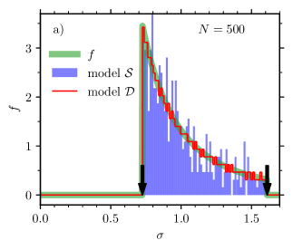
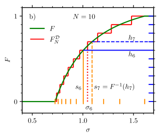
Figure 1: a) Histogram of $N=500$ particle diameters $\sigma_{i}$ of models $\mathcal{S}$ (blue) and $\mathcal{D}$ (red), respectively. For model $\mathcal{S}$ a single realization is shown, where each $\sigma_{i}$ is drawn independently from the density $f(\sigma)$ (green). In both histograms $70$ bins are used. The vertical arrows indicate the minimum and maximum diameters, $\sigma_{\rm m}$ and $\sigma_{\rm M}$, respectively. b) Cumulative distribution function (CDF) $F$ (green) and empirical CDF $F_{N}^{\mathcal{D}}$ for model $\mathcal{D}$ (red) as a function of diameter $\sigma$ for the example $N=10$. The diameters $\sigma_{i}$ are constructed from Eqs. (18-20), as graphically illustrated for $\sigma_{6}$.

Model $\mathcal{D}$. For model $\mathcal{D}$, we also use the CDF $F$ to obtain the particle diameters $\sigma_{i}$, $i=1,\dots,N$, but now we generate them in a deterministic manner. Our upcoming construction will satisfy the following three conditions:

1. The construction is deterministic. The system size $N$ uniquely defines the diameters,

   $$N~{}\mapsto~{}\sigma_{1},\dots,\sigma_{N}.$$ (14)

2. Convergence: The empirical CDF $F_{N}^{\mathcal{D}}$ approximates $F$. The convergence is uniform,

   $$\lim_{N\to\infty}F_{N}^{\mathcal{D}}\stackrel{{\scriptstyle\textit{uniform}}}{{=}}F\,.$$ (15)

   Thus the models $\mathcal{S}$ and $\mathcal{D}$ are consistent.

3. Constraint: For a given one-particle property $\theta(\sigma)$ of the diameter, the following constraint is fulfilled:

   $$\frac{1}{N}\sum_{i=1}^{N}\theta(\sigma_{i})=\mathrm{E}^{\mathcal{S}}[\,\theta\,].$$ (16)

   This means that the empirical mean of the function $\theta(\sigma_{i})$ equals the corresponding expectation $E^{\mathcal{S}}[\,\theta(\sigma_{i})\,]$ in model $\mathcal{S}$. To ensure this, $\theta$ is required to be a strictly monotonic function in $\sigma$.

For our work, we use $\theta(\sigma)=\frac{\pi}{6}\sigma^{3}$, inspired by the additive hard-sphere packing fraction, cf. Eq. (10). Here, Eq. (16) ensures that $\phi_{\mathrm{hs}}$ has the same value for any $N$,

$$\phi_{\mathrm{hs}}^{\mathcal{D}}=\mathrm{E}^{\mathcal{S}}[\phi_{\mathrm{hs}}]\equiv\phi_{\mathrm{hs}}^{\infty}.$$ (17)

So, how do we define the $N$ diameters $\sigma_{i}$ in the framework of model $\mathcal{D}$? First, we introduce $N+1$ equidistant nodes along the the codomain of $F$,

$$h_{i}=i/N, i=0,\dots,N.$$ (18)

Their pre-images $s_{i}$ are found on the domain of $F$,

$$s_{i}=F^{-1}(h_{i})\,.$$ (19)

We then define particle diameters $\sigma_{i}$, $i=1,\dots,N$, via

$$\theta(\sigma_{i})=N\int_{s_{i-1}}^{s_{i}}\theta(\sigma)f(\sigma)\,\mathrm{d}\sigma\,.$$ (20)

Since $\theta$ is assumed to be strictly monotonic, its inverse $\theta^{-1}$ exists and $\sigma_{i}$ is uniquely defined by Eq. (20). By summing over $i$ the constraint Eq. (16) is fulfilled. The proof of the uniform convergence $\lim_{N\to\infty}F_{N}^{\mathcal{D}}=F$ is presented in Appendix A. Note the analytical nature of the convergence for model $\mathcal{D}$ in contrast to the stochastic one for model $\mathcal{S}$, cf. Eq. (9).

Equation (20) with the choice $\theta(\sigma)=\frac{\pi}{6}\sigma^{3}$ is a sensible constraint for an additive hard-sphere system. For our non-additive soft-sphere system it is a minor tweak and not an essential condition. Another reasonable choice would be $\theta(\sigma)=\sigma$, which ensures that the empirical mean of the diameters exactly equals the unit of length $\bar{\sigma}$. Alternatively, one could ignore the constraint Eq. (16) and thus also Eq. (20) entirely and define $\sigma_{i}=s_{i}$ via Eq. (19) – note that one obtains $N+1$ diameters in this case. The latter approach was used in Ref. Santen and Krauth (2001). We expect that all these options are equivalent in the limit $N\to\infty$.

Figure 1a illustrates the distribution of diameters for the models $\mathcal{S}$ and $\mathcal{D}$. In each case, we show one histogram for $N=500$ particles, in comparison to the distribution density $f$. For a meaningful comparison, we have chosen the same number of 70 bins for both histograms. Since model $\mathcal{S}$ is of stochastic nature, we show the histogram for a single realization of diameters. In contrast, for model $\mathcal{D}$ the histogram at a given $N$ and bin number is uniquely defined (assuming an equidistant placement of bins on $[\sigma_{\mathrm{m}},\sigma_{\mathrm{M}}]$). The fluctuations around $f$ for model $\mathcal{S}$ appear to be larger than for $\mathcal{D}$. In the following paragraph “Order of convergence”, we put this finding on an analytical basis.

Figure 1b illustrates the construction of diameters $\sigma_{i}$ for model $\mathcal{D}$, based on the CDF $F$, for a small sample size $N=10$. For the resulting diameters the empirical CDF $F_{N}^{\mathcal{D}}$ is shown.

Order of convergence. Having established the convergence $\lim_{N\to\infty}F_{N}=F$ for models $\mathcal{S}$ and $\mathcal{D}$, we now compare their order of convergence. To this end, we calculate $\Delta F$, defined as the square-root of the mean squared deviation between $F_{N}$ and $F$,

$$\Delta F=(\mathrm{E}[(F_{N}-F)^{2}])^{1/2}\,.$$ (21)

Here, $\mathrm{E}[\,.\,]$ refers to the expectation with respect to the global diameter distribution. For model $\mathcal{D}$, the expectation $\mathrm{E}[\,.\,]$ is trivial and we obtain $\Delta F^{\mathcal{D}}=|F_{N}^{\mathcal{D}}-F|$. As shown in the Appendices A and B, the results for model $\mathcal{D}$ and $\mathcal{S}$ are respectively

$$\Delta F^{\mathcal{D}} \leq N^{-1}\,,$$ (22)

$$\Delta F^{\mathcal{S}} =\left((F(1-F)\right)^{1/2}N^{-1/2}\,.$$ (23)

This means that the order of convergence for model $\mathcal{D}$ is at least $1$, in contrast to model $\mathcal{S}$ where the order is only $1/2$. In this aspect, model $\mathcal{D}$ is superior to model $\mathcal{S}$, since its diameter distribution approaches the thermodynamic limit faster. Numerically, from the equations above, one has $\max_{\sigma}\Delta F^{\mathcal{D}}\leq\max_{\sigma}\Delta F^{\mathcal{S}}$ already for $N\geq 4$.

III Simulation details

Depending on the protocols introduced below, different particle-based simulation techniques are used, among which are molecular dynamics (MD) simulations, the Swap Monte Carlo (SWAP) method, and the coupling of the system to a Lowe-Andersen thermostat (LA).

In the MD simulations, Newton’s equations of motion are numerically integrated via the velocity form of the Verlet algorithm, using a time step of $\Delta t=0.01\,t_{0}$ (with $t_{0}=\bar{\sigma}\sqrt{m/u_{0}}$ setting the unit of time in the following). We employ the SWAP method in combination with MD simulation Berthier et al. (2019). To this end, every 25 MD steps, $N$ trial SWAP moves are performed. In a single SWAP move, a particle pair $(i,j)$ is randomly selected, followed by the attempt to exchange their diameters $(\sigma_{i},\sigma_{j})$ according to a Metropolis criterion. The probability $P_{\mathrm{SWAP}}$ to accept a SWAP trial as a function of $T$ is shown in Fig. 2. It indicates that even deep in the glassy state (far below the glass-transition temperature $T_{\rm g}^{\mathrm{SWAP}}\approx 0.06$, which we will define later on), the acceptance rate for a SWAP move is still $\gtrsim 4\%$ for $T\geq 0.01$. The latter is the lowest temperature shown here.

Figure 2: Acceptance rate $P_{\mathrm{SWAP}}$ of diameter exchange trials as a function of temperature $T$.

During the equilibration protocols, in each step, we couple the system to a Lowe-Andersen thermostat Koopman and Lowe (2006) for identical masses $m$ to reach a target temperature $T$: For each particle pair $(i,j)$ closer than a cutoff $R_{\mathrm{T}}$ and with a probability $\Gamma\Delta t$ new velocities are generated as

$${\bf v}_{i/j}^{\mathrm{new}}={\bf v}_{i/j}\pm\frac{1}{2}\left(\zeta\sqrt{\frac{2k_{B}T}{m}}-({\bf v}_{i}-{\bf v}_{j})\cdot\hat{\bf r}_{ij}\right)\hat{\bf r}_{ij},$$ (24)

where $\hat{\bf r}_{ij}=\mathbf{r}_{ij}/|\mathbf{r}_{ij}|$ and $\zeta$ is a normally distributed variable with expectation value of $0$ and variance of $1$. This means that only the component of the relative velocity parallel to $\hat{\bf r}_{ij}$ is thermalized, preserving the momentum as well as the angular momentum. We choose $R_{\mathrm{T}}=x_{c}$ and $\Gamma=4$.

Both for model $\mathcal{S}$ and model $\mathcal{D}$, we consider different system sizes $N=256$, $500$, $1000$, $2048$, $4000$, and $8000$ particles at different temperatures $T$, respectively. In each case, we prepare $60$ independent configurations as follows: The initial positions are given by a face-centered-cubic lattice (with cavities in case that $N\neq 4k^{3}$ for all integers $k$), while the initial velocities have a random orientation with a constant absolute value according to a high temperature $T=5$. The total momentum is set to $\bf{0}$ by subtracting $\sum_{i}{\bf v}_{i}/N$ from the velocity of each particle. The initial crystal is melted for a simulation time $t_{\text{max}}=2000$ with $\Delta t=0.001$, applying both the SWAP Monte Carlo and the LA thermostat. Then we cool the sample to $T=0.3$ for the same duration, followed by a run with $\Delta t=0.01$ over the time $t_{\text{max}}=10^{5}$ to fully equilibrate the sample at the target temperature $T$. After that we switch off SWAP (to ensure that the mean energy remains constant in the following) and measure a time series $H(t_{j})$ of the total energy over a time span of $0.75\,t_{\text{max}}$. Then we calculate the corresponding mean $H_{\mathrm{av}}$ and the standard deviation $\mathrm{sd}(H)$, and as soon as the condition $|H(t)-H_{\mathrm{av}}|<0.01\,\mathrm{sd}(H)$ is met, we switch off the LA thermostat and perform a microcanonical $NVE$ simulation for the remaining time up to $t=t_{\text{max}}$. This procedure reduces fluctuations in the final temperature $T$ for subsequent $NVE$ production runs.

For the analysis that we present in the following, we mostly compare $NVE$ with SWAP production runs (in both cases without the LA thermostat). Also, we perform MD production runs with the coupling to the LA thermostat but without applying the SWAP, and accordingly refer to these runs as the LA protocol. For all of these production runs, the initial configurations are the final samples obtained from the equilibration protocol described above.

For the LA thermostat and the SWAP Monte Carlo, pseudorandom numbers are generated by the Mersenne Twister algorithm Matsumoto and Nishimura (1998). For each sample, a different seed is chosen to ensure independent sequences. For an observable we eventually determine its $95\%$ confidence interval from its empirical CDF, which is calculated via Bootstrapping Efron (1992) with $1000$ repetitions.

IV Static fluctuations

In the following two subsections “Thermal fluctuations” and “Disorder fluctuations”, we consider two kinds of fluctuations. Thermal fluctuations quantify intrinsic fluctuations of phase-space variables for a given diameter configuration. These intrinsic observables are expected to coincide for both models $\mathcal{S}$ and $\mathcal{D}$, provided that $N$ is sufficiently large. As an example, we study thermal energy fluctuations, as quantified by the specific heat (here, numerical results are only shown for model $\mathcal{D}$). Below, we use this quantity to determine the glass-transition temperatures for the different dynamics.

In model $\mathcal{S}$, the dependence of thermally averaged observables on the diameter configuration leads to sample-to-sample fluctuations that are absent in model $\mathcal{D}$. We measure these fluctuations in terms of a disorder susceptibility, exemplified via the potential energy.

IV.1 Thermal fluctuations

Let us consider an $N$ particle sample of our system. An observable $O$ that characterizes the state of this sample depends in general on the particle coordinates $r=({\bf r}_{1},\dots,{\bf r}_{N}$), the momenta $p=({\bf p}_{1},\dots,{\bf p}_{N})$, and the particle diameters $\sigma=(\sigma_{1},\dots,\sigma_{N})$. When we denote the phase-space configuration by $q=(r,p)$, we can write the observable as $O=O(q,\sigma)$. Its thermal average can be expressed as

$$\langle O\rangle(\sigma)=\mathrm{E}(O|\sigma)=\int O(q,\sigma)\rho(q|\sigma)~{}\mathrm{d}q\,,$$ (25)

where $\rho(q|\sigma)$ is a conditional phase-space density. In the case of the canonical $NVT$ ensemble, it is given by

$$\rho(q|\sigma)=Z^{-1}\exp(-H(q|\sigma)/(k_{B}T))$$ (26)

with $Z=\int\exp(-H(q|\sigma)/(k_{B}T))~{}\mathrm{d}q$ the partition function and $H=K+U$ the Hamiltonian, cf. Sec. II.

In the simulations, we compute $\langle O\rangle(\sigma)$ via the average of an equidistant time sequence $q(t_{i})$ (with $\#t_{i}=5000$) over a time window $t_{\rm max}=10^{5}$. This approach is valid for an ergodic system - by definition - in case sufficient sampling is ensured. Then, the result does not depend on the initial condition $q(0)$. However, it does depend on the realization of $\sigma$ and, of course, the ensemble parameters, e.g. the temperature $T$.

Thermal fluctuations of the observable $O$ can be quantified in terms of the thermal susceptibility

$$\chi_{\mathrm{thm}}[O]=\mathrm{Var}(O|\sigma)/N=\langle O^{2}-\langle O\rangle^{2}\rangle/N\,.$$ (27)

Here the variance $\mathrm{Var}(\,.\,)$ is calculated according to the phase-space density (26). The normalization for $\chi_{\mathrm{thm}}$ is chosen such that for an extensive observable $O$ we expect finite values for $\lim_{N\to\infty}\chi_{\mathrm{thm}}[O]$.

An important quantity that is related to the thermal susceptibility of the potential energy $U$ is the excess specific heat at constant volume, defined by

$$C_{V}=\frac{1}{N}\frac{\partial\langle U\rangle}{\partial T}\,.$$ (28)

In the canonical $NVT$ ensemble, the relation between $C_{V}$ and the thermal susceptibility $\chi_{\mathrm{thm}}^{NVT}[U]$ is

$$C_{V}=\chi_{\mathrm{thm}}^{NVT}[U]/T^{2}\,.$$ (29)

This formula can be converted to the microcanonical $NVE$ ensemble to obtain Lebowitz et al. (1967)

$$C_{V}=\frac{\chi_{\mathrm{thm}}^{NVE}[U]}{T^{2}-(2/3)\chi_{\mathrm{thm}}^{NVE}[U]}\,.$$ (30)

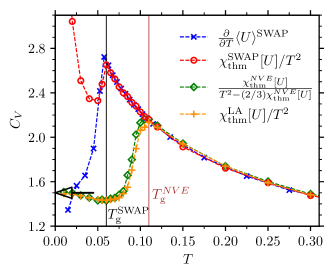
Figure 3: Specific heat $C_{V}$ as a function of temperature $T$ for model $\mathcal{D}$ with $N=2048$ particles. The solid lines indicate the glass-transition temperatures, corresponding to the microcanonical MD simulations (green, $T_{\mathrm{g}}^{NVE}=0.11$) and the simulations with SWAP dynamics (blue and red, $T_{\mathrm{g}}^{\mathrm{SWAP}}=0.06$). Coupling to the LA thermostat but without SWAP is represented by the orange line. The black arrow indicates the Dulong-Petit limit, $C_{V}=3/2$.

Figure 3 shows $C_{V}$ as a function of temperature $T$ for the different dynamics, namely the microcanonical MD via Eq. (30), the MD with SWAP using Eqs. (28) and (29), and the MD with LA thermostat employing again Eq. (29).

At high temperatures, $T\gtrsim 0.11$, the specific heat $C_{V}$ from the different calculations is in perfect agreement. Upon decreasing $T$, one observes relatively sharp drops in $C_{V}$ for the microcanonical $NVE$ and the SWAP dynamics. The drops occur at the temperatures $T_{\mathrm{g}}^{NVE}=0.11$ and $T_{\mathrm{g}}^{\mathrm{SWAP}}=0.06$, respectively, and indicate the glass transition of the different dynamics. These estimates of the glass-transition temperatures $T_{\mathrm{g}}$ are consistent with those obtained from dynamic correlation functions presented in Sec. V.

Another conclusion that we can draw from Fig. 3 is that fluctuations in $U$, as quantified by the $C_{V}$ from the SWAP dynamics simulations, correctly reproduce those in the canonical $NVT$ ensemble. This can be inferred from the coincidence of the blue and the red data points at temperatures $T>T_{\mathrm{g}}^{\mathrm{SWAP}}$. For the $NVE$ dynamics at $T<T_{\mathrm{g}}^{NVE}$, albeit using fully equilibrated samples as initial configurations for $T>T_{\mathrm{g}}^{\mathrm{SWAP}}$, relaxation times become too large to correctly resolve the fluctuations, as quantified by $\chi_{\mathrm{thm}}^{NVE}[U]$. We underestimate them within our finite simulation time and effectively measure a frequency-dependent specific heat Scheidler et al. (2001). Thus, from the monotonicity of Eq. (30), $C_{V}$ is underestimated as well. Furthermore, from the coincidence of the green with the orange data points, corresponding to the NVE and LA dynamics, respectively, we can conclude that the LA thermostat correctly reproduces the fluctuations in the canonical $NVT$ ensemble.

For the $NVE$ as well as LA dynamics, we see the Dulong-Petit law, i.e. for $T\to 0$ the specific heat approaches the value $C_{V}=3/2$. An exception to this finding are the results calculated from the SWAP dynamics. This can be understood by the fact that the SWAP dynamics are associated with fluctuating particle diameters even at very low temperatures; thus the resulting dynamics cannot be described in terms of the harmonic approximation for a frozen solid.

IV.2 Disorder fluctuations

In model $\mathcal{S}$, the Hamiltonian $H(q|\sigma)$ is parameterized by random variables $\sigma$ and this imposes a quenched disorder onto the system. This leads to fluctuations that can be quantified in terms of a disorder susceptibility that we shall define and analyze in this section.

To this end, we first introduce the diameter distribution density for both models,

$$g(\sigma) =\begin{cases}\Pi_{i=1}^{N}f(\sigma_{i}),&\mathrm{model}~{}\mathcal{S},\\ \Pi_{i=1}^{N}\delta_{\mathrm{D}}(\sigma_{i}-\sigma_{i}^{\mathcal{D}}),&\mathrm{model}~{}\mathcal{D}\,,\end{cases}$$ (31)

where $\delta_{\mathrm{D}}$ denotes the Dirac delta function.

Let us consider a variable $B=B(\sigma)$. This could be a function such as the additive hard-sphere packing fraction $\phi_{\mathrm{hs}}$ or the thermal average of a phase-space function at a given diameter configuration $\sigma$, e.g. $\langle U\rangle$. The disorder average of $B$, denoted by $\overline{B}$, is the expectation value of $B$ with respect to the distribution density $g$,

$$\overline{B}=\mathrm{E}(B)=\int B(\sigma)g(\sigma)~{}\mathrm{d}\sigma\,.$$ (32)

Note that in our analysis below, disorder averages are calculated by an average over all samples, i.e. over $60$ realizations of $\sigma$.

Fluctuations of an extensive quantity $B\sim N$ and its corresponding “density” $b=B/N$ can be measured by disorder susceptibilities, defined as

$$\chi_{\mathrm{dis}}[B] =\mathrm{Var}(B)/N=\overline{B^{2}-\overline{B}^{2}}/N\,,$$ (33)

$$\chi_{\mathrm{dis}}[b] =N\mathrm{Var}(b).$$ (34)

These two different definitions have to be applied for a meaningful scaling, i.e. to ensure $\chi_{\mathrm{dis}}[B]=\chi_{\mathrm{dis}}[b]$. For model $\mathcal{D}$, we have $\chi_{\mathrm{dis}}^{\mathcal{D}}[B]=0$ for any $B$. In contrast, for model $\mathcal{S}$ the variable $B(\sigma)$ fluctuates from sample to sample as quantified by $\chi_{\mathrm{dis}}[B]$. Here, in general, $\lim_{N\to\infty}\chi_{\mathrm{dis}}[B]\neq 0$, as exemplified by the fluctuations of the additive packing fraction: In Sec. II, we showed $\mathrm{Var}^{\mathcal{S}}(\phi_{\mathrm{hs}})\propto 1/N$, and thus we have $\chi^{\mathcal{S}}_{\mathrm{dis}}[\phi_{\mathrm{hs}}]=\textit{Const}>0$.

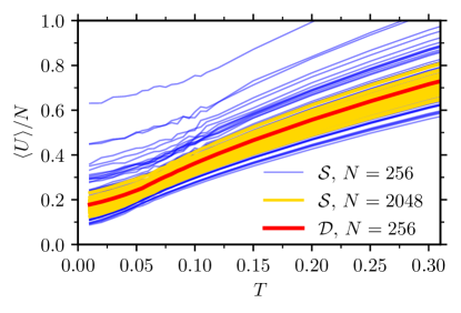
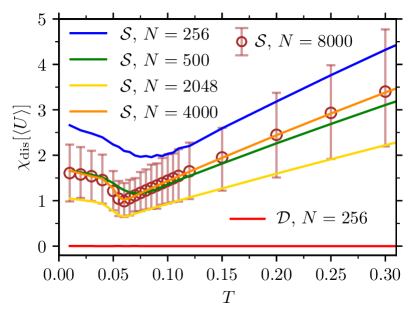
Figure 4: a) Mean potential energy $\langle U\rangle(\sigma)$ as a function of temperature $T$. For model $\mathcal{S}$, individual curves for each of the 60 samples are shown for systems with $N=256$ (blue lines) and $N=2048$ (orange lines) and for model $\mathcal{D}$ for the system with $N=256$. b) Disorder susceptibility $\chi_{\mathrm{dis}}[\langle U\rangle]$ for different values of $N$.

Potential energy. Having introduced the disorder average and susceptibility, we consider the variable $B(\sigma)=\langle U\rangle(\sigma)$, corresponding to the thermal average of the potential energy for a given sample with diameter configuration $\sigma$.

In Figure 4a the dependence of $\langle U\rangle(\sigma)$ on temperature $T$ is shown. For a given model and system size $N$, we present $60$ curves corresponding to $60$ independent samples. For model $\mathcal{S}$, results for $N=256$ and $2048$ are shown. Here, the diameter configurations $\sigma$ vary among the samples and thus, the potential energy fans out into various curves $\langle U\rangle(T)$. If we measure the fluctuations of the mean potential energy per particle, $\langle U\rangle(\sigma)/N$, with its variance, the fluctuations decrease with increasing $N$, as expected. For model $\mathcal{D}$, we show the curves of $60$ independent samples at $N=256$; here, sample-to-sample fluctuations are completely absent and all data collapse onto a single curve.

Figure 4b shows the disorder susceptibility $\chi_{\mathrm{dis}}[\langle U\rangle]$ of model $\mathcal{S}$ for different system sizes. As can be inferred from the figure, in a non-monotonous manner, $\chi_{\mathrm{dis}}[\langle U\rangle]$ seems to approach a finite temperature-dependent value in the limit $N\to\infty$,

$$\lim_{N\to\infty}\chi_{\mathrm{dis}}^{\mathcal{S}}[\langle U\rangle]=\textit{Constant}(T)>0\,.$$ (35)

Effective packing fraction. Now, we show that the disorder fluctuations in the potential energy $\langle U\rangle(\sigma)$ and the empirical limit value for $\chi_{\mathrm{dis}}^{\mathcal{S}}[\langle U\rangle]$, as given by Eq. (35), can be explained by fluctuations in a single scalar variable, namely an effective packing fraction $\phi_{\mathrm{eff}}$. The additive packing fraction $\phi_{\rm hs}$, cf. Eq. (10), is not an appropriate measure of a packing fraction for the non-additive soft-sphere system that we consider in this study. Therefore, we define an effective packing fraction $\phi_{\mathrm{eff}}$ to take into account the non-additivity of our model system.

The idea is to assign to each particle $i$ an “average” volume $V_{i}$ that accounts for the non-additive interactions. For this purpose, we first identify all $|\mathcal{N}_{i}|$ neighbors of $i$ within a given cutoff $r_{c}$,

$$\mathcal{N}_{i}=\left\{~{}j\in\{1,\dots,N\}~{}|~{}j\neq i,~{}r_{ij}<r_{c}\right\}\,.$$ (36)

Here $r_{c}=1.485$ is chosen, which corresponds to the location of the first minimum of the radial distribution function at the temperature $T=0.3$. Then, the volume $V_{i}$ of particle $i$ is defined as

$$V_{i}=\frac{1}{|\mathcal{N}_{i}|}\sum_{j\in\mathcal{N}_{i}}\frac{\pi}{6}\sigma_{ij}^{3}\,,$$ (37)

where non-additive diameters $\sigma_{ij}$ are given by Eq. (3).

Now we define an effective packing fraction $\phi_{\rm eff}$ as

$$\phi_{\mathrm{eff}}=V^{-1}\sum_{i=1}^{N}V_{i}\,.$$ (38)

Note that different from the hard-sphere packing fraction $\phi_{\rm hs}$, the value of the effective packing fraction $\phi_{\rm eff}$ of a given sample not only depends on the diameters $\sigma_{i}$, but it also depends on the coordinates ${\bf r}_{i}$. Thus, in our simulations of glassforming liquids, it is a thermally fluctuating variable. Therefore, we will use its thermal average $\langle\phi_{\mathrm{eff}}\rangle$ in our analysis below.

An alternative effective packing fraction can be defined by assigning an average diameter $S_{i}=\frac{1}{|\mathcal{N}_{i}|}\sum_{j\in\mathcal{N}_{i}}\sigma_{ij}$ instead of an average volume $V_{i}$ to each particle. The corresponding packing fraction is given by

$$\tilde{\phi}_{\mathrm{eff}}=V^{-1}\sum_{i=1}^{N}\frac{\pi}{6}S_{i}^{3}\,.$$ (39)

Below, we use the effective packing fractions $\phi_{\rm eff}$ and $\tilde{\phi}_{\rm eff}$ to analyse the sample-to-sample fluctuations in model $\mathcal{S}$. Although both definitions lead to similar results, we shall see that $\phi_{\rm eff}$ seems to provide a slightly better characterization of the thermodynamic state of the system than $\tilde{\phi}_{\rm eff}$.

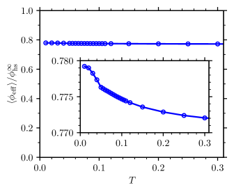
Figure 5: Reduced effective packing fraction $\langle\phi_{\mathrm{eff}}\rangle/\phi_{\rm hs}^{\infty}$ as a function of temperature $T$. The inset zooms into a region around $\langle\phi_{\mathrm{eff}}\rangle/\phi_{\rm hs}^{\infty}=0.775$.

Figure 5 displays the temperature dependence of $\langle\phi_{\mathrm{eff}}\rangle$. It is almost constant over the whole considered temperature range. This is a plausible result when one considers the weak temperature dependence of the structure of glassforming liquids. As we can infer from the inset of this figure, $\langle\phi_{\mathrm{eff}}\rangle$ increases mildly from about $0.772$ at $T=0.3$ to about $0.779$ at $T=0.01$.

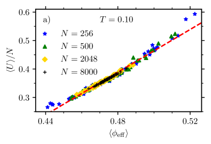
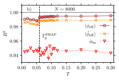
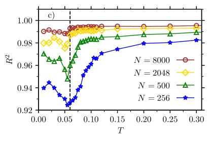
Figure 6: a) Scatter plot showing data points $\left(\langle\phi_{\rm eff}\rangle(\sigma)\,,\,\langle U\rangle(\sigma)/N\right)$ for model $\mathcal{S}$ at $T=0.10$ and different system sizes $N$. Each tuple belongs to a particular diameter realization $\sigma$. The red line is obtained via a linear-regression model $\phi\to\langle U\rangle$ with dependent variable $\langle U\rangle$ and regressor $\phi=\langle\phi_{\rm eff}\rangle$ for $N=2048$. Its coefficient of determination is $R^{2}\approx 0.984$. b) Coefficient of determination $R^{2}$ of the linear regression model $\phi\to\langle U\rangle$ as a function of $T$ for $N=8000$, using $\phi=\phi_{\mathrm{hs}}$ (red triangles), $\langle\phi_{\rm eff}\rangle$ (brown circles), and $\langle\tilde{\phi}_{\mathrm{eff}}\rangle$ (orange crosses) as regressors $\phi$. c) Similar to b), but here $R^{2}$ as a function of $T$ is shown for regressor $\phi=\langle\phi_{\rm eff}\rangle$ only, however for different system sizes $N$.

Now, we will use the variable $\langle\phi_{\mathrm{eff}}\rangle$ to quantify the sample-to-sample fluctuations of the potential energy per particle $\langle U\rangle(\sigma)/N$.

In Fig. 6a, we show $\langle U\rangle(\sigma)/N$ as a function of the mean packing fraction $\langle\phi_{\rm eff}\rangle(\sigma)$ at the temperature $T=0.10$. Here, we have used the data for $N=256$, $500$, and $2048$ particles. The plot suggests that the fluctuations of $\langle U\rangle$ can be explained by the variation of $\langle\phi_{\rm eff}\rangle$. We elaborate this finding by calculating the coefficient of determination $R^{2}$ of a linear-regression fit with dependent variable $\langle U\rangle/N$ and regressor $\langle\phi_{\rm eff}\rangle$.

In Fig. 6b we show $R^{2}$ as a function of $T$ for the system size $N=8000$. The linear regression analysis shows that approximately $99.5\%$ of the fluctuations can be explained by $\langle\phi_{\rm eff}\rangle$. This is a striking but physically plausible result, as it shows how a reduction from $N$ degrees of freedom given by $\sigma$ to one degree of freedom given by a thermodynamically relevant parameter $\langle\phi_{\rm eff}\rangle$ is sufficient to explain nearly all of the fluctuations. Also included in Fig. 6b is the coefficient of determination $R^{2}$ using $\phi=\phi_{\mathrm{hs}}$ and $\langle\tilde{\phi}_{\mathrm{eff}}\rangle$ as a regressor. While we obtain $R^{2}\approx 0.95$ for $\phi=\phi_{\mathrm{hs}}$, i.e. clearly below the value for $\langle\phi_{\rm eff}\rangle$, the value of $R^{2}$ for $\langle\tilde{\phi}_{\mathrm{eff}}\rangle$ is only slightly smaller, $R^{2}\approx 0.99$. Thus, among the three measures of the packing fraction, the variable $\langle\phi_{\rm eff}\rangle$ gives the best results. Note that the glass transition at $T_{\rm g}^{\rm SWAP}\approx 0.06$ is associated with a small drop of $R^{2}$ for the effective packing fractions.

Figure 6c displays the temperature dependence of $R^{2}$ for $\langle\phi_{\rm eff}\rangle$ for different system sizes $N$. The plot indicates a significant decrease of $R^{2}$ with decreasing $N$, especially at low temperatures around the glass-transition temperature $T_{\rm g}^{\rm SWAP}\approx 0.06$. The reason is that a linear relationship between $\langle U\rangle(\sigma)/N$ and $\langle\phi_{\rm eff}\rangle$ is expected to only hold in the vicinity of the disorder-averaged value $\overline{\langle\phi_{\mathrm{eff}}\rangle}$. For small system sizes, however, relatively large nonlinear deviations from this value occur that are reflected in a lower value of the coefficient of determination $R^{2}$. Moreover, for small $N$, the discretized nature of the diameter configuration does not any longer allow a description in terms of a single variable such as $\langle\phi_{\rm eff}\rangle$.

Our empirical results justify the idea to replace the dependency of $\langle U\rangle$ on the diameter configuration $\sigma$ by one on the single parameter $\langle\phi_{\rm eff}\rangle$,

$$\langle U\rangle(\sigma) \approx U^{*}\left(\langle\phi_{\mathrm{eff}}\rangle(\sigma)\right)$$

$$\approx U^{*}\left(\overline{\langle\phi_{\mathrm{eff}}\rangle}\right)+\frac{\partial U^{*}}{\partial\phi}\big{|}_{\phi=\overline{\langle\phi_{\mathrm{eff}}\rangle}}(\langle\phi_{\mathrm{eff}}\rangle-\overline{\langle\phi_{\mathrm{eff}}\rangle}).$$ (40)

Here $U^{*}$ is an unknown function in a scalar variable. According to the Taylor expansion above, fluctuations in $\langle U\rangle$ are inherited from those in $\langle\phi_{\mathrm{eff}}\rangle$ as

$$\mathrm{Var}(U^{*})\approx\left(\frac{\partial U^{*}}{\partial\phi}\right)^{2}\big{|}_{\phi=\overline{\langle\phi_{\mathrm{eff}}\rangle}}\mathrm{Var}(\langle\phi_{\mathrm{eff}}\rangle)\,.$$ (41)

Since $\langle\phi_{\mathrm{eff}}\rangle$ should scale similarly to the additive hard-sphere packing fraction $\phi_{\rm hs}$, we have $\mathrm{Var}(\langle\phi_{\mathrm{eff}}\rangle)\propto 1/N$. Then, since $U^{*}$ is extensive, Eq. (35) is confirmed.

V Structural Relaxation

In this section, the dynamic properties of the models $\mathcal{S}$ and $\mathcal{D}$ are compared. To this end, we analyze a time-dependent overlap function that measures the structural relaxation of the particles on a microscopic length scale. The timescale on which this function decays varies from sample to sample; these fluctuations around the average dynamics can be quantified in terms of a dynamic susceptibility. We shall see that the susceptibility in model $\mathcal{S}$ can be split into two terms. While the first term is due to thermal fluctuations and also present in model $\mathcal{D}$, the second term is due to the disorder in $\sigma$. At low temperatures, the contribution from the disorder can be the dominant term in the susceptibility.

For our analysis, we consider MD simulations in the microcanonical ensemble as well as hybrid simulations, combining MD with the Swap Monte Carlo technique (see Sec. III). In the following, we refer to these dynamics as “$NVE$” and “SWAP”, respectively.

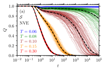
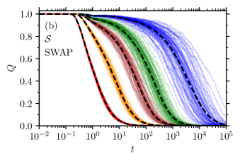
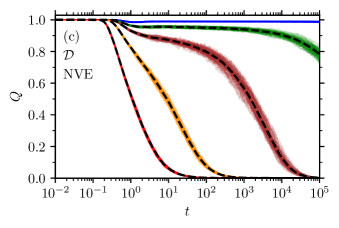
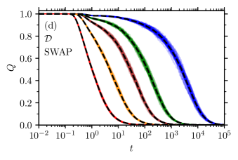
Figure 7: Overlap $Q(t)$ as a function of time $t$ for $NVE$ (left column) and SWAP dynamics (right column) for models $\mathcal{S}$ and $\mathcal{D}$. For the selected temperatures $T$ the initial configurations are in equilibrium. Solid colored lines represent $60$ individual simulations, while black dashed lines indicate their sample average. All results correspond to systems with $N=8000$ particles.

Glassy dynamics. A peculiar feature of the structural relaxation of glassforming liquids is the cage effect. On intermediate timescales, each particle gets trapped in a cage that is formed by its neighboring particles. To analyze structural relaxation from the cages, we therefore have to look at density fluctuations on a length scale $a$ similar to the size of the fluctuations of a particle inside such a cage. On a single-particle level, a simple time-dependent correlation function that measures the relaxation is the self part of the overlap function, defined by

$$Q(t)=\frac{1}{N}\sum_{i=1}^{N}\Theta(a-|{\bf r}_{i}(t)-{\bf r}_{i}(0)|)\,.$$ (42)

Here, we choose $a=0.3$ for the microscopic length scale. The behavior of $Q(t)$ is similar to that of the incoherent intermediate scattering function at a wave-number corresponding to the location of the first-sharp diffraction peak in the static structure factor. We note that we have not introduced any averaging in the definition (42). In the following, we will display the decay of $Q(t)$ for 60 individual samples at different temperatures. The corresponding initial configurations at $t=0$ were fully equilibrated with the aid of the SWAP dynamics before, as explained in Sec. III.

Figure 7 shows the overlap function $Q(t)$ for model $\mathcal{S}$ and model $\mathcal{D}$, in both cases for the $NVE$ and the SWAP dynamics. In all cases, we can see the typical signatures of glassy dynamics. At a high temperature, $T=0.3$, the function $Q(t)$ exhibits a monotonous decay to zero on a short microscopic timescale. Upon decreasing the temperature first a shoulder and then a plateau-like region emerges on intermediate timescales. This plateau extends over an increasing timescale with decreasing temperature and indicates the cage effect. Particles are essentially trapped within the same microstate in which they were initially at $t=0$. At the high temperature $T=0.3$ the decay of $Q(t)$ is very similar for $NVE$ and SWAP dynamics. Towards low temperatures, however, the decay is much faster in the case of the SWAP dynamics, as expected. A striking result is that at lower temperatures, the individual curves in model $\mathcal{S}$ show much larger variation than those in model $\mathcal{D}$. In the following, these sample-to-sample fluctuations shall be quantified in terms of a dynamic susceptibility.

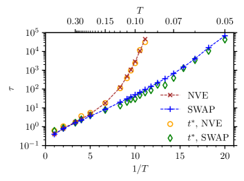
Figure 8: Relaxation time $\tau$, as extracted from the expectation of the overlap function, $\mathrm{E}[Q](t)$, and the time $t^{*}=\arg\max_{t}\chi(t)$, where the maximum of the dynamic susceptibility $\chi(t)$ occurs, for $NVE$ and SWAP dynamics. Here, a system with $N=8000$ particles is considered.

Relaxation time $\tau$. From the expectation of the overlap function, $\mathrm{E}[Q](t)$ (black dashed lines in Fig. 7), we extract an alpha-relaxation time $\tau$, defined by $\mathrm{E}[Q](\tau)=1/{\rm e}$. In Fig. 8, the logarithm of the timescale $\tau$ as a function of inverse temperature $1/T$ is shown. Also included in this plot are the times $t^{*}$ where the fluctuations of $Q(t)$ are maximal, which will be discussed in the following paragraph “Dynamic susceptibility”. One observes an increase of $\tau$ by about five orders of magnitude upon decreasing $T$. This increase is much quicker for the $NVE$ than for the SWAP dynamics, reflecting the fact that $T_{\rm g}^{\rm SWAP}$ is much lower than $T_{\rm g}^{NVE}$ (cf. Fig. 3). The glass-transition temperatures defined in Sec. IV via the drop in the specific heat $C_{V}(T)$ are approximately consistent with the alternative definition via $\tau(T_{\rm g})=10^{5}$.

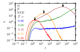
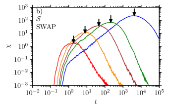
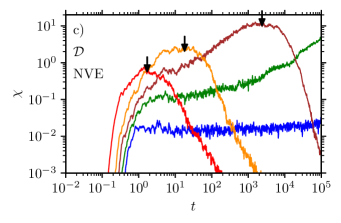
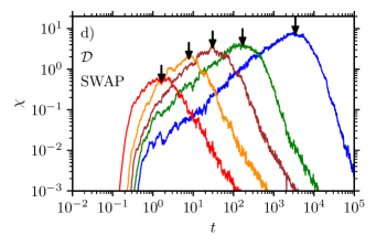
Figure 9: Dynamic susceptibility $\chi$ as a function of time $t$ for different temperatures $T$ and systems with $N=8000$ particles. Results for all four combinations of $NVE$ and SWAP dynamics with models $\mathcal{S}$ and $\mathcal{D}$ are shown, as labeled in a)-d). Maxima of $\chi(t)$ are marked by arrows. Prior to their calculation we performed a moving average over the raw data.

Dynamic susceptibility $\chi(t)$. A characteristic feature of glassy dynamics is the presence of dynamical heterogeneities that are associated with large fluctuations around the “average” dynamics. These fluctuations can be quantified in terms of a dynamic (or four-point) susceptibility. For the overlap function $Q(t)$, this susceptibility $\chi(t)$ can be defined as

$$\chi(t)=N\mathrm{Var}\left(Q(t)\right)\,.$$ (43)

The function $\chi(t)$ measures the fluctuations of $Q(t)$ around the average $\mathrm{E}[Q](t)$. In practice, we use the data of $Q(t)$ from the ensemble of 60 independent samples.

Figure 9 shows the dynamic susceptibility $\chi(t)$ for the same cases as for $Q(t)$ in Fig. 7. As a common feature of glassy dynamics Chandler et al. (2006); Cavagna (2009), $\chi(t)$ exhibits a peak $\chi^{*}:=\mathrm{max}_{t}~{}\chi(t)$ at $t=t^{*}$. The timescale $t^{*}$ is roughly equal to the alpha-relaxation time $\tau$, see Fig. 8. At the temperatures $T=0.1$ for the $NVE$ and $T=0.06$ for the SWAP dynamics, $\chi^{*}$ is more than one order of magnitude larger for model $\mathcal{S}$ than for model $\mathcal{D}$. This indicates that the disorder in $\sigma$ of model $\mathcal{S}$ strongly affects the sample-to-sample fluctuations. In the following paragraph “Variance decomposition” we will present how one can distinguish disorder from thermal fluctuations.

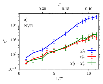
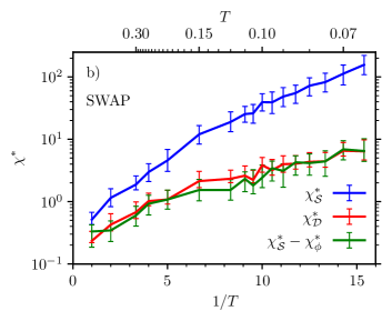
Figure 10: Maximum of the dynamic susceptibility, $\chi^{*}=\mathrm{max}_{t}\chi(t)$, as a function of $1/T$ for a) the $NVE$ and b) the SWAP dynamics. Results are shown for models $\mathcal{S}$ (blue line) and $\mathcal{D}$ (red line) with $N=8000$ particles. The green solid line displays $\chi_{\mathcal{S}}^{*}-\chi_{\phi}^{*}$, i.e. the total susceptibility minus the explained part caused by the packing-fraction fluctuations.

Figure 10 shows the maximum of the dynamic susceptibility, $\chi^{*}$, as a function of inverse temperature, $1/T$, for $NVE$ and SWAP dynamics. In both cases, the results for model $\mathcal{S}$ ($\chi_{\mathcal{S}}^{*}$) and model $\mathcal{D}$ ($\chi_{\mathcal{D}}^{*}$) are included, considering systems with $N=8000$ particles. In all cases $\chi^{*}$ increases with decreasing temperature $T$, as expected for glassy dynamics. For both types of dynamics the difference $\Delta\chi^{*}=\chi_{\mathcal{S}}^{*}-\chi_{\mathcal{D}}^{*}$ increases with decreasing temperature as well. The lowest temperatures for which we can calculate $\Delta\chi^{*}$ are (i) $T=0.09$ with a relative deviation $\Delta\chi^{*}/\chi^{*}_{\mathcal{D}}\approx 18$ for the $NVE$ and (ii) $T=0.065$ with $\Delta\chi^{*}/\chi^{*}_{\mathcal{D}}\approx 23$ for the SWAP dynamics.

Variance decomposition. To understand the difference $\Delta\chi^{*}$ between $\chi_{\mathcal{S}}$ and $\chi_{\mathcal{D}}$, we will decompose the dynamic susceptibility $\chi_{\mathcal{S}}$ of model $\mathcal{S}$ into one term that stems from the thermal fluctuations of the phase-space variables, and a second term that is caused by the sample-to-sample variation of the diameters $\sigma$.

As a matter of fact, in model $\mathcal{S}$ the overlap function $Q(t)$ and similar correlation functions depend on two random vectors, namely the initial phase-space point $q_{0}=\left(r(0),v(0)\right)$ and the diameters $\sigma$. As a consequence, we define and calculate $\chi=N\mathrm{Var}(Q)$ on a probability space with respect to the joint-probability density

$$\rho(q_{0},\sigma)=\rho(q_{0}|\sigma)g(\sigma).$$ (44)

Here $\rho(q_{0}|\sigma)$ is the conditional phase-space density introduced in Eq. (26) and $g(\sigma)$ is the diameter distribution defined by Eq. (31).

Now, since $Q$ depends on two random vectors $q_{0}$ and $\sigma$, we can decompose $\chi=N\mathrm{Var}(Q)$ according to the variance decomposition formula, also called law of total variance or Eve’s law Chung (1974):

$$\mathrm{Var}(Q) =\mathrm{E}\left[\mathrm{Var}(Q|\sigma)\right]+\mathrm{Var}\left(\mathrm{E}[Q|\sigma]\right)$$ (45)

$$\equiv\overline{\langle Q^{2}-\langle Q\rangle^{2}\rangle}+\overline{\langle Q\rangle^{2}-\overline{\langle Q\rangle}^{2}}\,.$$ (46)

Here, $\mathrm{E}\left[\mathrm{Var}(Q|\sigma)\right]$ describes intrinsic thermal fluctuations, while the term $\mathrm{Var}\left(\mathrm{E}[Q|\sigma]\right)$ expresses fluctuations induced by the disorder in $\sigma$.

The first summand in Eq. (45) is expected to coincide for both models $\mathcal{S}$ and $\mathcal{D}$ for sufficiently large $N$, as $\mathrm{Var}(Q|\sigma)$ describes intrinsic thermal fluctuations for a given realization of $\sigma$, which are calculated via the model-independent conditional phase-space density $\rho(q_{0}|\sigma)$. The physical observable $\mathrm{Var}(Q|\sigma)$ should not depend on microscopic details of the diameter configuration $\sigma$ for sufficiently large $N$. For the cumulative distribution functions of the diameters, the consistency equation $\lim_{N\to\infty}F_{N}^{\mathcal{S}}(s)=F(s)=\lim_{N\to\infty}F_{N}^{\mathcal{D}}(s)$ holds. Thus, we expect that $\mathrm{E}^{\mathcal{S}}\left[\mathrm{Var}(Q|\sigma)\right]\approx\mathrm{E}^{\mathcal{D}}\left[\mathrm{Var}(Q|\sigma)\right]$. This equation should be exact in the limit $N\to\infty$. We have implicitly used this line of argument also in Sec. IV, where we have only shown numerical results of the specific heat for model $\mathcal{D}$. Furthermore, for model $\mathcal{D}$ we have exactly $\mathrm{E}^{\mathcal{D}}[\mathrm{Var}(Q|\sigma)]=\mathrm{Var}(Q|\sigma^{\mathcal{D}})=\mathrm{Var}^{\mathcal{D}}(Q)$, since here there is only one diameter configuration $\sigma=\sigma^{\mathcal{D}}$ for a given system size $N$.

Summarizing the results above, we can express the dynamic susceptibility for model $\mathcal{S}$ as follows:

$$\mathrm{Var}^{\mathcal{S}}(Q)=\mathrm{Var}^{\mathcal{D}}(Q)+\mathrm{Var}^{\mathcal{S}}\left(\mathrm{E}[Q|\sigma]\right).$$ (47)

Now the aim is to estimate the second summand in Eq. (47). We assume that we can describe the disorder in $\sigma$ by a single parameter, namely the thermally averaged effective packing fraction $\langle\phi_{\rm eff}\rangle(\sigma)$, defined by Eq. (38). This idea has been already proven successful in Sec. IV, when we described the disorder fluctuations of the potential energy. Similarly, we write

$$\mathrm{E}[Q|{\sigma}]\equiv\langle Q\rangle(\sigma)\approx Q^{*}({\langle\phi_{\rm eff}\rangle}(\sigma))\,,$$ (48)

assuming that the values of $\langle Q\rangle(\sigma)$, which depend on $N$ degrees of freedom, can be described by a function $Q^{*}$ that only depends on a scalar argument, the scalar-valued function $\langle\phi_{\rm eff}\rangle(\sigma)$. The function $Q^{*}$ is unknown, but can be estimated numerically with a linear-regression analysis, predicting $\langle Q\rangle$ with the regressor $\langle\phi_{\rm eff}\rangle$. Insertion of Eq. (48) into Eq. (47) gives

$$\mathrm{Var}^{\mathcal{S}}(Q)\approx\mathrm{Var}^{\mathcal{D}}(Q)+\mathrm{Var}^{\mathcal{S}}(Q^{*}(\langle\phi_{\rm eff}\rangle))\,.$$ (49)

We can write this equation in terms of susceptibilities,

$$\chi_{\mathcal{S}} ~{}\approx\chi_{\mathcal{D}}+\chi_{\mathcal{\phi}},$$ (50)

$$\chi_{\mathcal{\phi}} :=N\mathrm{Var}^{\mathcal{S}}(Q^{*}(\langle\phi_{\rm eff}\rangle)).$$ (51)

Along the lines of Eq. (41) in Sec. IV, we can expand the overlap function $Q^{*}$ around $\overline{\langle\phi_{\rm eff}\rangle}$ to obtain

$$\mathrm{Var}^{\mathcal{S}}(Q^{*}(\langle\phi_{\rm eff}\rangle)\approx\mathrm{Var}^{\mathcal{S}}(\langle\phi_{\rm eff}\rangle)\,\left(\frac{\partial Q^{*}(\phi)}{\partial\phi}\big{|}_{\phi=\overline{\langle\phi_{\mathrm{eff}}\rangle}}\right)^{2}.$$ (52)

Since $\mathrm{Var}^{\mathcal{S}}(\langle\phi_{\rm eff}\rangle)\sim\mathrm{Var}^{\mathcal{S}}(\phi_{\rm hs})\propto N^{-1}$ and $Q^{*}\sim Q\in\mathcal{O}(1)$, this equation implies that the susceptibility $\chi_{\phi}$, to leading order, does not depend on $N$. Moreover, for a given temperature $T$ and time $t$, it approaches a constant value in the thermodynamic limit, $N\to\infty$. For small system sizes, however, higher-order corrections to Eq. (52) cannot be neglected. Beyond that, the discretized nature of the system at small $N$ will lead to a failure of the “continuity-assumption” (48) itself. Finite-size effects of $\chi$ will be analyzed in the following paragraph.

In Fig. 10, we show for the system with $N=8000$ particles that $\chi_{\phi}^{*}$, i.e. $\chi_{\phi}$ evaluated at $t=t^{*}$, indeed captures the sample-to-sample fluctuations in model $\mathcal{S}$ due to the disorder in $\sigma$. Both for $NVE$ and SWAP dynamics, it quantitatively describes the gap between $\chi_{\mathcal{S}}^{*}$ and $\chi_{\mathcal{D}}^{*}$.

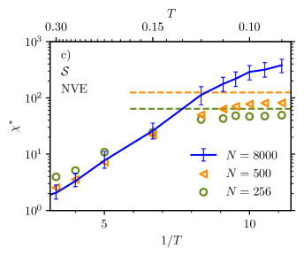
Figure 11: $\chi_{\mathcal{S}}^{*}$ as a function of $1/T$ for different system sizes $N$ using $NVE$ dynamics. The dashed lines denote $N/4$, which is the upper bound according to Popoviciou’s inequality on variances, see Eq. (53).

Finite-size effects: Popoviciou’s inequality on variances. Here, we analyze finite-size effects of the dynamic susceptibility $\chi$. To this end, we again consider the temperature dependence of the maximum of the dynamic susceptibility, $\chi^{*}$, considering only the case of the $NVE$ dynamics. Note that for model $\mathcal{D}$ finite-size effects in the considered temperature range $0.09\leq T\leq 0.3$ are negligible; therefore we only discuss model $\mathcal{S}$ in the following.

Figure 11 shows $\chi_{\mathcal{S}}^{*}$ as a function of $1/T$ for $N=256$, 500, and 8000. At high temperatures $T$, where fluctuations are small, there is hardly, if any, dependency on the system size $N$. However, upon lowering $T$ a saturation occurs at least for the small systems. This behavior can be understood by a hard stochastic upper limit on fluctuations, which is given by Popoviciou’s inequality on variances Popoviciu (1935). This inequality is valid for any bounded real-valued random variable $X$: Let $c$ and $C$ be the lower and upper bound of $X$, respectively, then Popoviciou states that $\mathrm{Var}(X)\leq(C^{2}-c^{2})/4$. Applying this result to $X=Q$ with sharp boundaries $c=0$ and $C=1$ yields

$$\chi\equiv N\mathrm{Var}(Q)\leq N/4.$$ (53)

Our data shows that this upper bound is quite sharp for $N=256$ and $N=500$ at low $T$. This can be understood by the fact that the equality of the inequality (53) holds precisely when $Q$ is a Bernoulli variable, i.e. when there are exactly two outcomes $Q=0$ or $Q=1$ each with probability $1/2$. In this sense, the saturation of $\chi$ should occur at temperatures $T$ and system sizes $N$ at a given $t$ when $Q(t)$ for approximately half of the samples has decayed close to $0$ while for the other half $Q$ is still close to $1$.

The inequality (53) is very useful to estimate how large a system size $N$ needs to be to avoid this kind of finite-size effect: All one has to do is to compare the measured $\chi$ at a given $N$ to the number $\chi_{c}:=N/4$. In the case that $\chi\approx\chi_{c}$, one has to consider larger system sizes $N$.

VI Summary and conclusions

In this work, we use molecular dynamics (MD) computer simulation in combination with the SWAP Monte Carlo technique to study a polydisperse model glassformer that has recently been introduced by Ninarello et al. Ninarello et al. (2017). Two methods are used to choose the particle diameters $\sigma_{1},\dots,\sigma_{N}$ to obtain samples with $N$ particles. Both of these approximate the desired distribution density $f(\sigma)\sim\sigma^{-3}$ with their histogram. In model $\mathcal{S}$ the diameters are drawn from $f(\sigma)$ in a stochastic manner. In model $\mathcal{D}$ the diameters are obtained via a deterministic scheme that assigns an appropriate set of $N$ values to them. We systematically compare the properties of model $\mathcal{S}$ to those of model $\mathcal{D}$ and investigate how the sample-to-sample variation of the diameters in model $\mathcal{S}$ affects various quantities: (i) classical phase-space functions such as the potential energy $U$ and its fluctuations, and (ii) dynamic correlation functions such as the overlap function $Q(t)$ and its fluctuations as well.

Obviously, model $\mathcal{D}$ has the advantage that always “the most representative sample” Santen and Krauth (2001) is used for any system size $N$, while model $\mathcal{S}$ may suffer from statistical outliers, especially in the case of small $N$. This indicates that the quenched disorder introduced by the different diameter configurations in model $\mathcal{S}$ may strongly affect fluctuations that we investigate systematically in this work.

Our main findings can be summarized as follows: The sample-to-sample fluctuations in model $\mathcal{S}$ can be described in terms of a single scalar parameter, namely the effective packing fraction $\langle\phi_{\rm eff}\rangle(\sigma)$, defined by Eq. (38). In terms of this parameter, one can explain the disorder fluctuations of the potential energy (cf. Fig. 6) as well as the gap between the dynamic susceptibilities of models $\mathcal{S}$ and $\mathcal{D}$ (cf. Fig. 10). The sample-to-sample fluctuations of the potential energy in model $\mathcal{S}$ can be quantified in terms of the disorder susceptibility $\chi_{\mathrm{dis}}^{\mathcal{S}}$ which is a non-trivial function of temperature (cf. Fig. 4) and finite in the thermodynamic limit $N\to\infty$. In model $\mathcal{S}$, at very low temperatures, the dynamic susceptibility is dominated by the fluctuations due to the diameter disorder. Thus, if one is aiming at analyzing the “true” dynamic heterogeneities of a glassformer, that stem from the intrinsic thermal fluctuations, one may preferentially use model $\mathcal{D}$. Note that it is possible to calculate the same thermal susceptibility in model $\mathcal{S}$ as in model $\mathcal{D}$, however the calculation in $\mathcal{S}$ is more difficult, as it demands an additional average over the disorder, as shown in Sec. V. This implies that model $\mathcal{S}$ requires more sampling in this case.

Our findings are of particular importance regarding recent simulation studies of polydisperse glassforming systems in external fields Guiselin et al. (2020a, b); Lamp et al. (2022); Lerner (2019); Rainone et al. (2020) where a model $\mathcal{S}$ approach was used to select the particle diameters. However, in these works sample-to-sample fluctuations due to the disorder in $\sigma$ have been widely ignored. Exceptions are the studies by Lerner et al. Lerner (2019); Rainone et al. (2020) where samples whose energy deviates from the mean energy by more than 0.5% were just discarded. Here the use of a model $\mathcal{D}$ scheme would be a more efficient alternative. However, one should still keep in mind that with regard to a realistic description of experiments on polydisperse colloidal systems, it might be more appropriate to choose model $\mathcal{S}$.

Appendix A Convergence of the CDF $F_{N}^{\mathcal{D}}$

Here, we prove that the empirical cumulative distribution function (CDF) $F_{N}^{\mathcal{D}}$ of model $\mathcal{D}$, see Eqs. (8) and (20), converges uniformly to the exact CDF $F$, defined by Eq. (6). As we shall see below, the order of convergence is at least $1$. For the strictly monotonic function $\theta$, that we have introduced in Sec. II, we assume that it is strictly increasing, but the proof is analogous for a strictly decreasing $\theta$.

In the first step, we show that

$$\sigma_{i}\in[s_{i-1},s_{i}], i=1,\dots,N.$$ (54)

Starting point is Eq. (20) from which we estimate

$$\theta(\sigma_{i}) \leq N\int_{s_{i-1}}^{s_{i}}\theta(s_{i})f(\sigma)~{}\mathrm{d}\sigma$$ (55)

$$=N\theta(s_{i})\int_{s_{i-1}}^{s_{i}}f(\sigma)~{}\mathrm{d}\sigma$$ (56)

$$=N\theta(s_{i})[F(s_{i})-F(s_{i-1})]$$ (57)

$$=N\theta(s_{i})\left[\frac{i}{N}-\frac{i-1}{N}\right]=\theta(s_{i}).$$ (58)

Since $\theta$ is strictly increasing, its inverse $\theta^{-1}$ exists and is strictly increasing, too. Applying $\theta^{-1}$ to the inequality above yields $\sigma_{i}\leq s_{i}$. Similarly, we obtain $\sigma_{i}\geq s_{i-1}$. This confirms Eq. (54).

In the second step, we consider an arbitrary $\epsilon>0$ and natural numbers $N\geq N_{0}$ with $N_{0}=\lceil\epsilon^{-1}\rceil$. Now we select $\sigma\in\mathbb{R}$. For $\sigma<\sigma_{\rm m}$ or $\sigma>\sigma_{\rm M}$, we trivially have $F_{N}^{\mathcal{D}}(\sigma)=F(\sigma)$. In the remaining case $\sigma_{\rm m}\leq\sigma\leq\sigma_{\rm M}$, an index $i$ exists such that $s_{i-1}\leq\sigma\leq s_{i}$. The latter statement is true, because the union of all intervals $[s_{i-1},s_{i}]$ yields the total interval $[\sigma_{\rm m},\sigma_{\rm M}]$. From Eq. (54) it follows that there are exactly $i$ or $i-1$ particles with $\sigma_{i}\leq\sigma$, so that $F_{N}^{\mathcal{D}}(\sigma)=i/N$ or $F_{N}^{\mathcal{D}}(\sigma)=(i-1)/N$, respectively.

In the third step, we point out that $F(\sigma)$ is a monotonously increasing function so that

$$\frac{i-1}{N}=F(s_{i-1})\leq F(\sigma)\leq F(s_{i})=\frac{i}{N}.$$ (59)

Subtracting $F_{N}^{\mathcal{D}}(\sigma)$ yields

$$|F_{N}^{\mathcal{D}}(\sigma)-F(\sigma)|\leq 1/N\leq 1/N_{0}<\epsilon\,.$$ (60)

This proves the uniform convergence

$$\lim_{N\to\infty}F_{N}^{\mathcal{D}}=F$$ (61)

of the order of convergence of at least $1$.

Appendix B Convergence of the CDF $F_{N}^{\mathcal{S}}$

To find the order of convergence for $\lim_{N\to\infty}F_{N}^{\mathcal{S}}=F$ of model $\mathcal{S}$, we measure deviations by $\Delta F=(\mathrm{E}^{\mathcal{S}}[(F_{N}^{\mathcal{S}}-F)^{2}])^{1/2}$, see Eq. (21). We first calculate

$$(F_{N}^{\mathcal{S}}-F)^{2} =\frac{1}{N^{2}}\sum_{i=1}^{N}\sum_{j=1}^{N}(\mathbf{1}_{i}-F)(\mathbf{1}_{j}-F),$$ (62)

$$\mathbf{1}_{i}(\sigma) :=\mathbf{1}_{\left(-\infty,\sigma\right]}(\sigma_{i}).$$ (63)

Here, we abbreviated the full notation of the indicator function $\mathbf{1}$. Its expectation is given by

$$\mathrm{E}^{\mathcal{S}}[\mathbf{1}_{i}(\sigma)] =1\,P(\sigma_{i}\leq\sigma)+0\,P(\sigma_{i}>\sigma)=F(\sigma).$$ (64)

Here, $P$ denotes the appropriate probability for model $\mathcal{S}$. When calculating the expectation $\mathrm{E}^{\mathcal{S}}$ of Eq. (62), only the diagonal terms $i=j$ remain due to the stochastic independence of the diameters $\sigma_{i}$ and $\sigma_{j}$ for $i\neq j$. We end up with

$$\mathrm{E}^{\mathcal{S}}[(F_{N}^{\mathcal{S}}-F)^{2}] =F(1-F)N^{-1},$$ (65)

$$\Rightarrow\Delta F^{\mathcal{S}} =\left((F(1-F)\right)^{1/2}\,N^{-1/2}.$$ (66)

This means the order of convergence for model $\mathcal{S}$ is only $1/2$. Concerning the prefactor, we have $\max_{\sigma}F(1-F)=1/4$ at the $\sigma$ where $F(\sigma)=1/2$. Thus it is

$$\max_{\sigma}\Delta F^{\mathcal{S}}=\frac{1}{2}N^{-1/2}.$$ (67)

Note that no inequality is used in the calculations above and thus the order of convergence is sharp.

References

- Gasser (2009) U. Gasser, Journal of Physics: Condensed Matter 21, 203101 (2009).
- van Megen and Underwood (1993) W. van Megen and S. M. Underwood, Physical Review Letters 70, 2766 (1993).
- van Megen and Underwood (1994) W. van Megen and S. M. Underwood, Physical Review E 49, 4206 (1994).
- Schöpe et al. (2006) H.-J. Schöpe, G. Bryant, and W. van Megen, Physical Review E 74, 060401(R) (2006).
- Schöpe et al. (2007) H.-J. Schöpe, G. Bryant, and W. van Megen, Journal of Chemical Physics 127, 084505 (2007).
- Pham et al. (2002) K. N. Pham, A. M. Puertas, J. Bergenholtz, S. U. Egelhaaf, A. Moussaïd, P. N. Pusey, A. B. Schofield, M. E. Cates, M. Fuchs, and W. C. K. Poon, Science 296, 104 (2002).
- Pusey et al. (2009) P. N. Pusey, E. Zaccarelli, C. Valeriani, E. Sanz, W. C. K. Poon, and M. E. Cates, Philosophical Transactions of the Royal Society A 367, 4993 (2009).
- Zaccarelli et al. (2015) E. Zaccarelli, S. M. Liddle, and W. C. K. Poon, Soft Matter 11, 324 (2015).
- Brambilla et al. (2009) G. Brambilla, D. El Masri, M. Pierno, L. Berthier, L. Cipelletti, G. Petekidis, and A. B. Schofield, Physical Review Letters 102, 085703 (2009).
- Klochko et al. (2020) L. Klochko, J. Baschnagel, J. P. Wittmer, O. Benzerara, C. Ruscher, and A. N. Semenov, Physical Review E 102, 042611 (2020).
- Leocmach et al. (2013) M. Leocmach, J. Russo, and H. Tanaka, Journal of Chemical Physics 138, 12A536 (2013).
- Ingebrigtsen and Tanaka (2015) T. S. Ingebrigtsen and H. Tanaka, Journal of Physical Chemistry B 119, 11052 (2015).
- Ingebrigtsen et al. (2021) T. S. Ingebrigtsen, T. B. Schrøder, and J. C. Dyre, Journal of Physical Chemistry B 125, 317 (2021).
- Ninarello et al. (2017) A. Ninarello, L. Berthier, and D. Coslovich, Physical Review X 7, 021039 (2017).
- Guiselin et al. (2020a) B. Guiselin, G. Tarjus, and L. Berthier, The Journal of Chemical Physics 153, 224502 (2020a).
- Vaibhav et al. (2022) V. Vaibhav, J. Horbach, and P. Chaudhuri, Journal of Chemical Physics 156, 244501 (2022).
- Lamp et al. (2022) K. Lamp, N. Küchler, and J. Horbach, Journal of Chemical Physics 157, 034501 (2022).
- Voigtmann and Horbach (2009) T. Voigtmann and J. Horbach, Physical Review Letters 103, 205901 (2009).
- Weysser et al. (2010) F. Weysser, A. M. Puertas, M. Fuchs, and T. Voigtmann, Physical Review E 82, 011504 (2010).
- Santen and Krauth (2001) L. Santen and W. Krauth, arXiv preprint cond-mat/0107459 (2001).
- Tsai et al. (1978) N.-H. Tsai, F. F. Abraham, and G. Pound, Surface Science 77, 465 (1978).
- Grigera and Parisi (2001) T. S. Grigera and G. Parisi, Physical Review E 63, 045102(R) (2001).
- Guiselin et al. (2020b) B. Guiselin, L. Berthier, and G. Tarjus, Physical Review E 102, 042129 (2020b).
- Berthier et al. (2019) L. Berthier, E. Flenner, C. J. Fullerton, C. Scalliet, and M. Singh, Journal of Statistical Mechanics: Theory and Experiment 2019, 064004 (2019).
- Koopman and Lowe (2006) E. Koopman and C. Lowe, The Journal of chemical physics 124, 204103 (2006).
- Matsumoto and Nishimura (1998) M. Matsumoto and T. Nishimura, ACM Transactions on Modeling and Computer Simulation (TOMACS) 8, 3 (1998).
- Efron (1992) B. Efron, in Breakthroughs in statistics (Springer, 1992), pp. 569–593.
- Lebowitz et al. (1967) J. Lebowitz, J. Percus, and L. Verlet, Physical Review 153, 250 (1967).
- Scheidler et al. (2001) P. Scheidler, W. Kob, A. Latz, J. Horbach, and K. Binder, Physical Review B 63, 104204 (2001).
- Chandler et al. (2006) D. Chandler, J. P. Garrahan, R. L. Jack, L. Maibaum, and A. C. Pan, Phys. Rev. E 74, 051501 (2006), URL https://link.aps.org/doi/10.1103/PhysRevE.74.051501.
- Cavagna (2009) A. Cavagna, Physics Reports 476, 51 (2009).
- Chung (1974) K. L. Chung, A Course in Probability Theory (Academic Press, New York, 1974).
- Popoviciu (1935) T. Popoviciu, Mathematica 9, 20 (1935).
- Lerner (2019) E. Lerner, Journal of Non-Crystalline Solids 522, 119570 (2019), ISSN 0022-3093, URL https://www.sciencedirect.com/science/article/pii/S0022309319304417.
- Rainone et al. (2020) C. Rainone, E. Bouchbinder, and E. Lerner, Proceedings of the National Academy of Sciences 117, 5228 (2020), eprint https://www.pnas.org/doi/pdf/10.1073/pnas.1919958117, URL https://www.pnas.org/doi/abs/10.1073/pnas.1919958117.