Slimmable Networks for Contrastive Self-supervised Learning

Abstract

Self-supervised learning makes significant progress in pre-training large models, but struggles with small models. Previous solutions to this problem rely mainly on knowledge distillation, which involves a two-stage procedure: first training a large teacher model and then distilling it to improve the generalization ability of smaller ones. In this work, we present a one-stage solution to obtain pre-trained small models without the need for extra teachers, namely, slimmable networks for contrastive self-supervised learning (SlimCLR). A slimmable network consists of a full network and several weight-sharing sub-networks, which can be pre-trained once to obtain various networks, including small ones with low computation costs. However, interference between weight-sharing networks leads to severe performance degradation in self-supervised cases, as evidenced by gradient magnitude imbalance and gradient direction divergence. The former indicates that a small proportion of parameters produce dominant gradients during backpropagation, while the main parameters may not be fully optimized. The latter shows that the gradient direction is disordered, and the optimization process is unstable. To address these issues, we introduce three techniques to make the main parameters produce dominant gradients and sub-networks have consistent outputs. These techniques include slow start training of sub-networks, online distillation, and loss re-weighting according to model sizes. Furthermore, theoretical results are presented to demonstrate that a single slimmable linear layer is sub-optimal during linear evaluation. Thus a switchable linear probe layer is applied during linear evaluation. We instantiate SlimCLR with typical contrastive learning frameworks and achieve better performance than previous arts with fewer parameters and FLOPs.

1 Introduction

Over the last decade, deep learning achieves significant success in various fields of artificial intelligence, primarily due to a significant amount of manually labeled data. However, manually labeled data is expensive and far less available than unlabeled data in practice. To overcome the constraint of costly annotations, self-supervised learning (Dosovitskiy et al., 2016; Wu et al., 2018; van den Oord et al., 2018; He et al., 2020; Chen et al., 2020a) aims to learn transferable representations for downstream tasks by training networks on unlabeled data. There has been significant progress in large models, which are larger than ResNet-50 (He et al., 2016) that has roughly 25M parameters. For example, ReLICv2 (Tomasev et al., 2022) achieves an accuracy of 77.1% on ImageNet (Russakovsky et al., 2015) under a linear evaluation protocol with ResNet-50, outperforming the supervised baseline 76.5%.

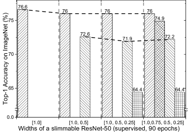
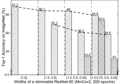
Figure 1: A slimmable ResNet-50 in supervised (left) and self-supervised (right) manners. $\text{ResNet-50}_{[1.0,0.75,0.5,0.25]}$ means this slimmbale network can switch at width $[1.0,0.75,0.5,0.25]$. The width ${0.25}$ represents that the number of channels is scaled by $0.25$ of the full network.

In contrast to the success of the large model pre-training, self-supervised learning with small models lags behind. For instance, supervised ResNet-18 with 12M parameters achieves an accuracy of 72.1% on ImageNet, but its self-supervised result with MoCov2 (Chen et al., 2020c) is only 52.5% (Fang et al., 2021). The gap is nearly 20%. To bridge the significant performance gap between supervised and self-supervised small models, previous methods (Koohpayegani et al., 2020; Fang et al., 2021; Gao et al., 2022; Xu et al., 2022) mainly focus on knowledge distillation, where they attempt to transfer the knowledge of a self-supervised large model into small ones. Nevertheless, such methodology has a two-stage procedure: first train an additional large model, and then train a small model to mimic the large one. Moreover, one-time distillation only produces a single small model for a specific computation scenario.

An interesting question arises: can we obtain multiple small models through one-time pre-training to meet various computation scenarios without the need for additional teachers? Inspired by the success of slimmable networks in supervised learning (Yu et al., 2019; Yu and Huang, 2019b, a), we develop a novel one-stage method for obtaining pre-trained small models without extra large models: slimmable networks for contrastive self-supervised learning, referred to as SlimCLR. A slimmable network comprises a full network and several weight-sharing sub-networks with different widths, where the width represents the number of channels in a network. The slimmable network can operate at various widths, allowing flexible deployment on different computing devices. Therefore, we can obtain multiple networks, including small ones for low computing scenarios, through one-time pre-training. Weight-sharing networks can also inherit knowledge from large ones via shared parameters, resulting in better generalization performance.

Weight-sharing networks in a slimmable network cause interference with each other when training simultaneously, particularly in self-supervised cases. In Figure 1, weight-sharing networks only have a slight impact on each other under supervision, with the full model achieving 76.6% vs. 76.0% accuracy in $\text{ResNet-50}_{[1.0]}$ and $\text{ResNet-50}_{[1.0,0.75,0.5,0.25]}$. However, without supervision, the corresponding numbers become 67.2% vs. 64.8%. The observed evidence of interference among weight-sharing networks includes gradient magnitude imbalance and gradient direction divergence. Gradient magnitude imbalance occurs when a small proportion of parameters produce dominant gradients during backpropagation. This happens because the shared parameters receive gradients from multiple losses of different networks, which can result in the majority of parameters not being fully explored. Gradient direction divergence refers to the situation where the gradient directions of the full network are disordered, resulting in an unstable optimization process. In self-supervised cases, weighting-sharing networks may produce diverse outputs without strong constraints such as labels in supervised cases, leading to conflicts in gradient directions.

To alleviate gradient magnitude imbalance, it is essential to ensure that the main parameters generate dominant gradients during backpropagation. To avoid conflicts in gradient directions of weight-sharing networks, they should have consistent outputs. To achieve these goals, we propose three simple yet effective techniques during pre-training to alleviate interference among networks. 1) We adopt a slow start strategy for sub-networks. The networks and pseudo supervision of contrastive learning are both unstable and fast updating at the start of training. To avoid interference making the situation worse, we only train the full model initially. After the full model becomes relatively stable, sub-networks can inherit learned knowledge via shared parameters and begin with better initialization. 2) We apply online distillation to make all sub-networks consistent with the full model, thereby eliminating the gradient divergence of networks. The predictions of the full model serve as consistent guidance for all sub-networks. 3) We re-weight the losses of networks according to their widths to ensure that the full model dominates the optimization process. Additional, theoretical results are provided to demonstrate that a single slimmable linear layer is sub-optimal during linear evaluation. Therefore, we adopt a switchable linear probe layer to avoid the interference caused by parameter-sharing.

We instantiate two algorithms for SlimCLR with typical contrastive learning frameworks, i.e., MoCov2 (Chen et al., 2020c) and MoCov3 (Chen et al., 2021). Extensive experiments on ImageNet (Russakovsky et al., 2015) show that SlimCLR achieves significant performance improvements compared to previous arts with fewer parameters and FLOPs.

2 Related Works

2.1 Self-supervised learning 

Self-supervised learning aims to learn transferable representations for downstream tasks from the input data itself. According to Liu et al. (2020), self-supervised methods can be summarized into three main categories according to their objectives: generative, contrastive, and generative-contrastive (adversarial). Methods belonging to the same categories can be further classified by the difference between pretext tasks. Given input $x$, generative methods encode $x$ into an explicit vector $z$ and decode $z$ to reconstruct $x$ from $z$, e.g., auto-regressive (van den Oord et al., 2016a, b), auto-encoding models (Ballard, 1987; Kingma and Welling, 2014; Devlin et al., 2019; He et al., 2022). Contrastive learning methods encoder input $x$ into an explicit vector $z$ to measure similarity. The two mainstream methods below this category are context-instance contrast (infoMax Hjelm et al. (2019), CPC van den Oord et al. (2018), AMDIM Bachman et al. (2019)) and instance-instance contrast (DeepCluster Caron et al. (2018), MoCo  He et al. (2020); Chen et al. (2021), SimCLR  Chen et al. (2020a, b), SimSiam Chen and He (2021)). Generative-contrastive methods generate a fake sample $x^{\prime}$ from $x$ and try to distinguish $x^{\prime}$ from real samples, e.g., DCGANs Radford et al. (2016), inpainting Pathak et al. (2016), and colorization Zhang et al. (2016).

2.2 Slimmable networks

Slimmable networks are first proposed to achieve instant and adaptive accuracy-efficiency trade-offs on different devices (Yu et al., 2019). A slimmable network can execute at different widths during runtime. Following the pioneering work, universally slimmable networks (Yu and Huang, 2019b) develop systematic training approaches to allow slimmable networks to run at arbitrary widths. AutoSlim (Yu and Huang, 2019a) further achieves one-shot architecture search for channel numbers under a certain computation budget. MutualNet (Yang et al., 2020) trains slimmable networks using different input resolutions to learn multi-scale representations. Dynamic slimmable networks (Li et al., 2022, 2021) change the number of channels of each layer on the fly according to the input. In contrast to weight-sharing sub-networks in slimmable networks, some methods aim to train multiple sub-networks with independent parameters (Zhao et al., 2022b). A relevant concept of slimmable networks in network pruning is network slimming (Liu et al., 2017; Chavan et al., 2022; Wang et al., 2021), which aims to achieve channel-level sparsity for better computation efficiency.

2.3 Knowledge distillation

Knowledge distillation (Hinton et al., 2015) aims to transfer the knowledge learned by a large network to a smaller one, and can be roughly categorized into two types: logits distillation (Hinton et al., 2015; Zhang et al., 2018; Guo, 2022; Zhao et al., 2022a; Mirzadeh et al., 2020) and intermediate feature distillation (Park et al., 2019; Tian et al., 2020; Peng et al., 2019). The former only requires the student to mimic the output of the teacher, while the latter also aligns the intermediate features of the teacher and student. Intermediate feature distillation methods generally achieve better performance than logits distillation methods. Recently, several methods (Guo, 2022; Zhao et al., 2022a) try to find out the limit of logits distillation and improve its performance. In this paper, online distillation is a kind of logits distillation. Besides, in a slimmable network, distillation also occurs between a large network and a small network via the shared parameters.

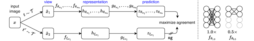
(a) left: SlimCLR-MoCov2. right: a slimmable network with two widths $[1.0,0.5]$.

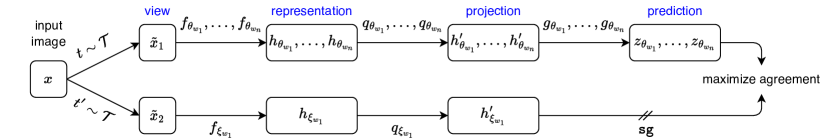
(b) SlimCLR-MoCov3

Figure 2: The overall framework of SlimCLR. A slimmable network produces different outputs from weight-sharing networks with various widths $w_{1},\ldots,w_{n}$, where $w_{1}$ is the width of the full model. $\theta$ are the network parameters and $\xi$ are an exponential moving average of $\theta$. $\mathtt{sg}$ means stop-gradient.

3 Method

3.1 Description of SlimCLR

We develop two instantial algorithms for SlimCLR with typical contrastive learning frameworks MoCov2 and MoCov3 (Chen et al., 2020c, 2021). As shown in Figure 2(a) (right), a slimmable network with $n$ widths ${w_{1}},\ldots,{w_{n}}$ contains multiple weight-sharing networks $f_{\theta_{w_{1}}},\ldots,f_{\theta_{w_{n}}}$, which are parameterized by learnable weights ${\theta_{w_{1}}},\ldots,{\theta_{w_{n}}}$, respectively. Each network $f_{\theta_{w_{i}}}$ in the slimmable network has its own set of weights $\Theta_{w_{i}}$ and $\theta_{w_{i}}\in\Theta_{w_{i}}$. A network with a small width shares the weights with large ones, namely, $\Theta_{w_{j}}\subset\Theta_{w_{i}}$ if $w_{j}<w_{i}$. Generally, we assume $w_{j}<w_{i}$ if $j>i$, i.e., $w_{1},\ldots,w_{n}$ arrange in descending order, and $\theta_{w_{1}}$ represent the parameters of the full model.

We first illustrate the learning process of SlimCLR-MoCov2 in Figure 2(a). Given a set of images $\mathcal{D}$, an image $x$ sampled uniformly from $\mathcal{D}$, and one distribution of image augmentation $\mathcal{T}$, SlimCLR produces two data views $\tilde{x}_{1}=t(x)$ and $\tilde{x}_{2}=t^{\prime}(x)$ from $x$ by applying augmentations $t\sim\mathcal{T}$ and $t^{\prime}\sim\mathcal{T}$, respectively. For the first view, SlimCLR outputs multiple representations $h_{\theta_{w_{1}}},\ldots,h_{\theta_{w_{n}}}$ and predictions $z_{\theta_{w_{1}}},\ldots,z_{\theta_{w_{n}}}$  , where $h_{\theta_{w_{i}}}=f_{\theta_{w_{i}}}(\tilde{x}_{1})$ and $z_{\theta_{w_{i}}}=g_{\theta_{w_{i}}}(h_{\theta_{w_{i}}})$. $g$ is a stack of slimmable linear transformation layers, i.e., a slimmable version of the MLP head in MoCov2 and SimCLR (Chen et al., 2020a). For the second view, SlimCLR only outputs a single representation from the full model $h_{\xi_{w_{1}}}=f_{\xi_{w_{1}}}(\tilde{x}_{2})$ and prediction $z_{\xi_{w_{1}}}=g_{\xi_{w_{1}}}(h_{\xi_{w_{1}}})$. We minimize the InfoNCE (van den Oord et al., 2018) loss with respect to $\theta_{w_{i}}$ to maximize the similarity of positive pairs $z_{\theta_{w_{i}}}$ and $z_{\xi_{w_{1}}}$:

$$\mathcal{L}_{\theta_{w_{i}}}=-\log\frac{\mathrm{e}^{\overline{z}_{\xi_{w_{1}}}\cdot\frac{\overline{z}_{\theta_{w_{i}}}}{\tau_{1}}}}{\mathrm{e}^{\overline{z}_{\xi_{w_{1}}}\cdot\frac{\overline{z}_{\theta_{w_{i}}}}{\tau_{1}}}+\sum_{z^{-}}\mathrm{e}^{z^{-}\cdot\frac{\overline{z}_{\theta_{w_{i}}}}{\tau_{1}}}},$$ (1)

where $\overline{z}_{\theta_{w_{i}}}=z_{\theta_{w_{i}}}/\lVert z_{\theta_{w_{i}}}\rVert_{2}$, $\overline{z}_{\xi_{w_{1}}}=z_{\xi_{w_{1}}}/\lVert z_{\xi_{w_{1}}}\rVert_{2}$, $\tau_{1}$ is a temperature hyper-parameter, and $\{z^{-}\}$ are features of negative samples. In SlimCLR-MoCov2, $\{z^{-}\}$ are obtained from a queue which is updated every iteration during training by $\overline{z}_{\xi_{w_{1}}}$, following the approach used in MoCov2. Without any regularization during training, the overall objective is the sum of losses of all networks with various widths:

$$\mathcal{L}_{\theta}=\sum_{i=1}^{n}\mathcal{L}_{\theta_{w_{i}}}.$$ (2)

Here $\xi$ is updated by $\theta$ every iteration using a momentum coefficient $m\in[0,1)$, as follows: $\xi\leftarrow m\xi+(1-m)\theta$.

Compared to SlimCLR-MoCov2, SlimCLR-MoCov3 has an additional projection process. Firstly, it projects the representation to another high dimensional space, then makes predictions. The projector $q$ is a stack of slimmable linear transformation layers. SlimCLR-MoCov3 also adopts the InfoNCE loss, but the negative samples come from other samples in the mini-batch.

After contrastive learning, we only keep $f_{\theta_{w_{1}}},\ldots,f_{\theta_{w_{n}}}$ and abandon other components.

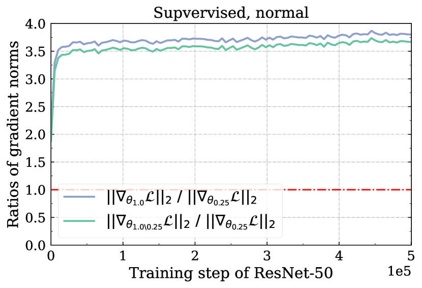
(a) 76.6%

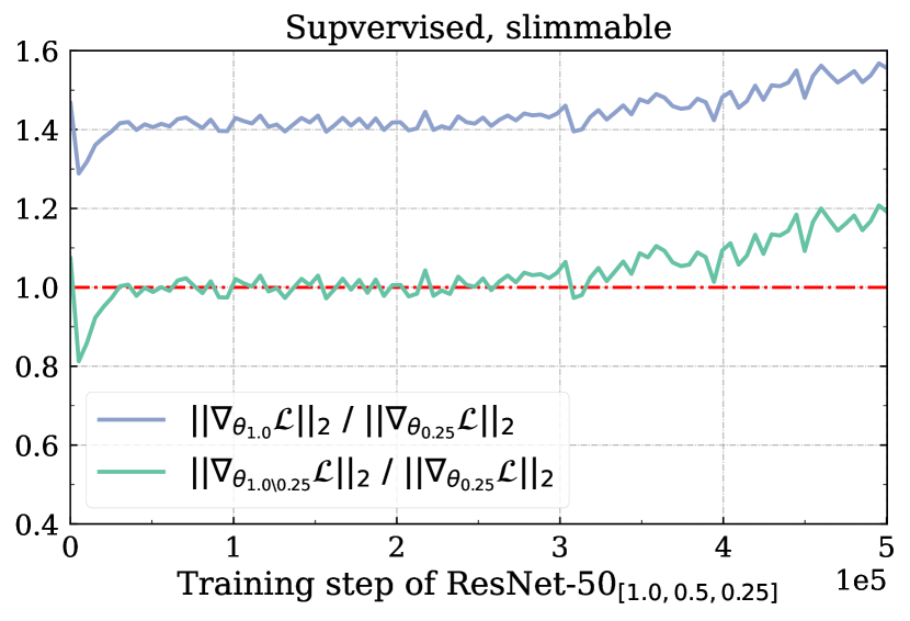
(b) 76.0%, 72.9%, 64.4%

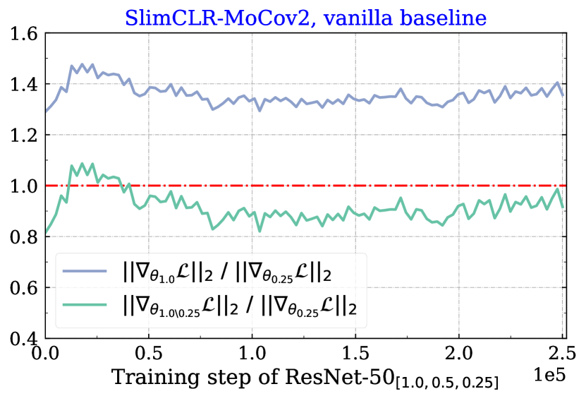
(c) 66.0%, 61.4%, 54.5%

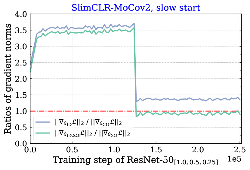
(d) 66.3%, 62.2%, 55.1%

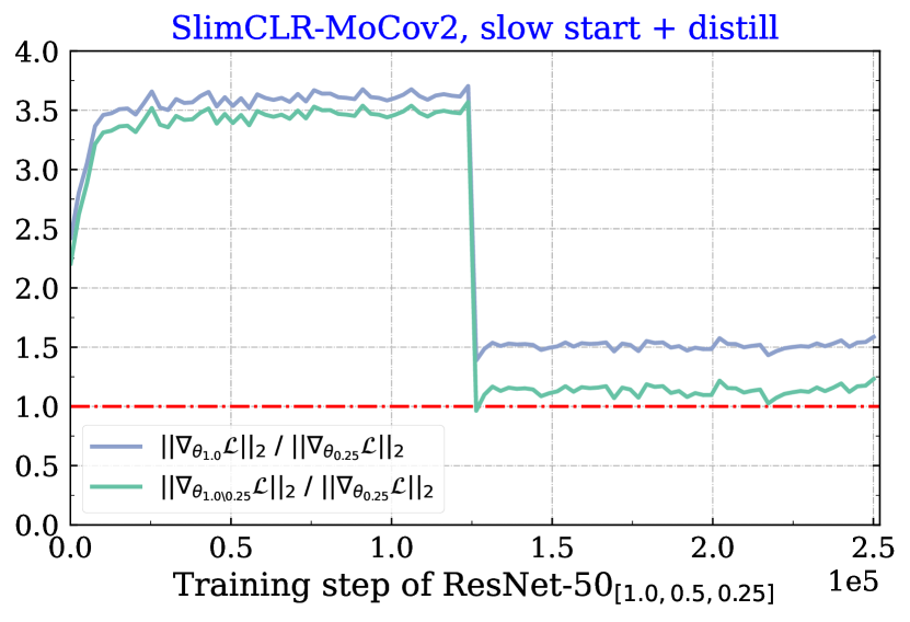
(e) 66.9%, 62.3%, 54.9%

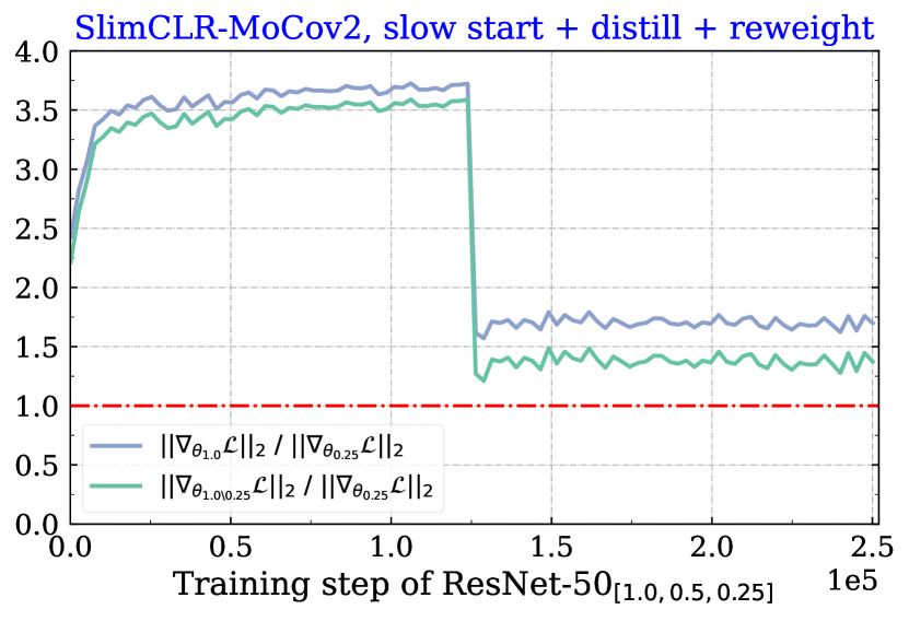
(f) 67.0%, 62.4%, 55.1%

Figure 3: Ratios of gradient norms: $\frac{\lVert\nabla_{\theta_{1.0}}\mathcal{L}_{\theta}\rVert_{2}}{\lVert\nabla_{\theta_{0.25}}\mathcal{L}_{\theta}\rVert_{2}}$ and $\frac{\lVert\nabla_{\theta_{1.0\backslash 0.25}}\mathcal{L}_{\theta}\rVert_{2}}{\lVert\nabla_{\theta_{0.25}}\mathcal{L}_{\theta}\rVert_{2}}$. The gradient norm of the network is calculated by averaging the layer-wise $\ell_{2}$ gradient norms. $\nabla_{\theta_{1.0\backslash 0.25}}\mathcal{L}_{\theta}$ is the gradient of the final loss w.r.t. parameters $\theta_{1.0\backslash 0.25}\in\Theta_{1.0}\backslash\Theta_{0.25}$, i.e., rest parameters of $\Theta_{1.0}$ besides $\Theta_{0.25}$.

3.2 Interference of networks and solutions

In Figure 1, it can be observed that a vanilla implementation of SlimCLR suffers from significant performance degradation due to interference of weight-sharing networks. In this section, we will discuss the consequences of this interference and present solutions to address it.

Gradient magnitude imbalance

Gradient magnitude imbalance refers to the phenomenon where a small fraction of parameters receives dominant gradients during backpropagation. For example, in a slimmable network with widths $[1.0,0.5,0.25]$, $\ell 2$ norm of $\theta_{0.25}$ — $\lVert\nabla_{\theta_{0.25}}\mathcal{L}_{\theta}\rVert_{2}$ maybe larger than that of the remaining parameters $\lVert\nabla_{\theta_{1.0\backslash 0.25}}\mathcal{L}_{\theta}\rVert_{2}$, even though $\theta_{0.25}$ only counts for approximately $6\%$ of the total parameters. This is because the gradients of different losses accumulate as follows:

$$\nabla_{\theta_{w_{n}}}\mathcal{L}_{\theta}=\frac{\partial\mathcal{L}_{\theta}}{\partial\theta_{w_{n}}}=\sum_{i=1}^{n}\frac{\partial\mathcal{L}_{\theta_{w_{i}}}}{\partial{\theta_{w_{n}}}}.$$ (3)

Assuming that the gradients of a single loss have a similar magnitude distribution, the accumulation of gradients from different losses increases the gradient norm of the shared parameters.

We evaluate the gradient magnitude imbalance by calculating the ratios of gradient norms during training. Figure 3 shows the ratios of $\lVert\nabla_{\theta_{1.0}}\mathcal{L}_{\theta}\rVert_{2}$ and $\lVert\nabla_{\theta_{1.0\backslash 0.25}}\mathcal{L}_{\theta}\rVert_{2}$ versus $\lVert\nabla_{\theta_{0.25}}\mathcal{L}_{\theta}\rVert_{2}$, separately. The ratio of their numbers of parameters is $\frac{\lvert{\Theta_{1.0}\backslash\Theta_{0.25}}\rvert}{\lvert{\Theta_{0.25}}\rvert}\approx 15$, where $\theta_{1.0\backslash 0.25}\in\Theta_{1.0}\backslash\Theta_{0.25}$. In Figure 3(a), both ratios of gradient norms are around 3.5, indicating that the majority of parameters obtain a large gradient norm and dominate the optimization process. However, in Figure 3(b) & 3(c), when training a slimmable network with widths $[1.0,0.5,0.25]$, $\lVert\nabla_{\theta_{0.25}}\mathcal{L}_{\theta}\rVert_{2}$ becomes close or larger than $\lVert\nabla_{\theta_{1.0\backslash 0.25}}\mathcal{L}_{\theta}\rVert_{2}$ despite having much fewer parameters.

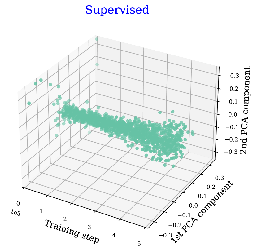
(a) supervised R-50_{[1.0,0.5,0.25]}

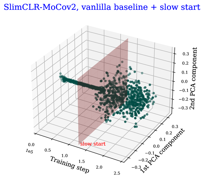
(b) SlimCLR-MoCov2

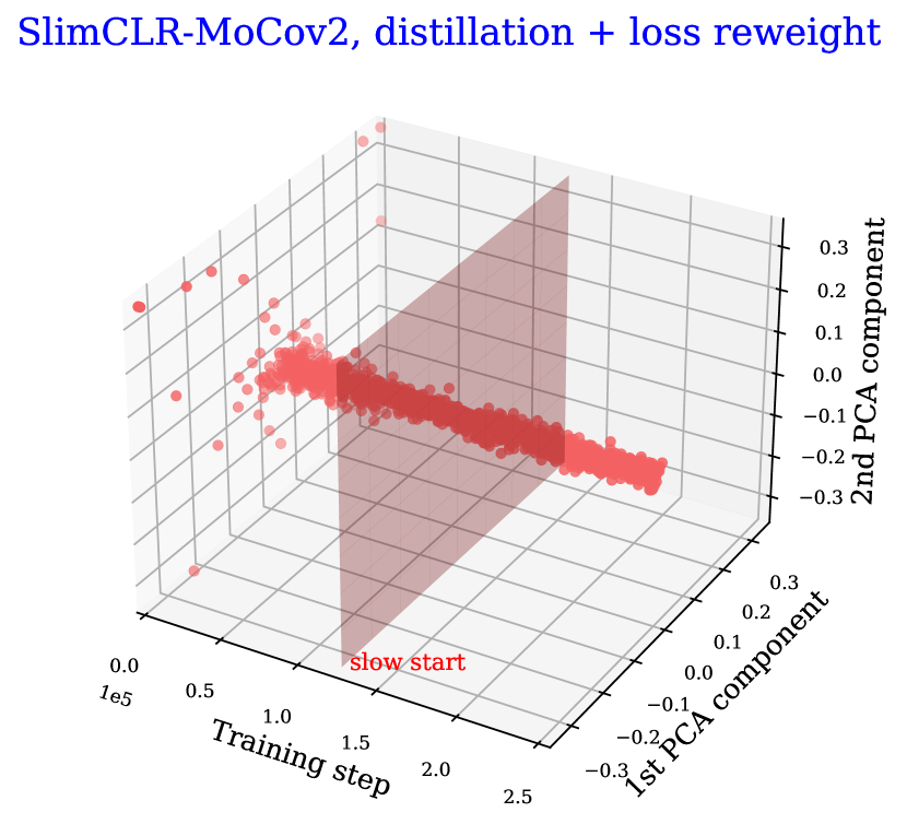
(c) SlimCLR-MoCov2

Figure 4: Gradient direction divergence. The principal gradient directions of the last linear layer are shown.

Gradient magnitude imbalance is more pronounced in self-supervised cases. In the case of supervised learning shown in Figure 3(b), $\lVert\nabla_{\theta_{1.0\backslash 0.25}}\mathcal{L}_{\theta}\rVert_{2}$ is is initially close to $\lVert\nabla_{\theta_{0.25}}\mathcal{L}_{\theta}\rVert_{2}$, but the former increases as training progresses. By contrast, for vanilla SlimCLR-MoCov2 in Figure 3(c), $\lVert\nabla_{\theta_{1.0\backslash 0.25}}\mathcal{L}_{\theta}\rVert_{2}$ is smaller than the other most time. A conjecture is that the pretext task — instance discrimination is more challenging than supervised classification. Consequently, small networks with limited capacity face difficulty in converging, leading to large losses and dominant gradients.

Gradient direction divergence

In addition to the imbalance in gradient magnitudes, the gradient directions of different weight-sharing networks can also conflict with each other. These conflicts lead to disordered gradient directions of the full model, which we refer to as gradient direction divergence.

We visualize the principal gradient directions in Figure 4. Specifically, we collect the gradients with respect to parameters in the last linear layer during training; after training, we perform PCA on these gradients and calculate their projections on the first two principal components (Li et al., 2018). In Figure 4(b), before the slow start point, we only train the full model. In this case, the gradient directions are stable and consistent during training. By contrast, after the slow start point, gradient directions become disordered due to conflicts in weight-sharing networks. We also show the gradient directions when training a slimmable network in a supervised case in Figure 4(a). In the supervised case, gradient direction divergence is also inevitable. Nevertheless, the gradient direction divergence in the supervised case is less significant compared to the self-supervised case in Figure 4(b). In supervised cases, all networks have consistent global supervision during training. By contrast, in self-supervised cases, the negative samples in Eq. (1) are always changing during training, and the optimization goal is not consistent throughout the training process. Additionally, since the predictions of weight-sharing networks may vary significantly from each other, this can result in different similarity scores in Eq. (1) and divergent gradient directions. These factors exacerbate the phenomenon of gradient direction divergence in self-supervised cases.

Solutions to network interference

To address the issue of gradient magnitude imbalance, it is necessary for the majority of parameters to dominate the optimization process, namely, the ratios of gradient norms in Figure 3 should be large. To alleviate the problem of gradient direction divergence, constraints can be placed on the similarity scores in Eq. (1) to prevent predictions from varying significantly from each other. To achieve these goals, we develop three simple yet effective pre-training techniques: slow start, online distillation, and loss reweighting. Furthermore, we provide theoretical evidence demonstrating that a weight-sharing linear layer is suboptimal during linear evaluation, and a switchable linear probe layer is a better alternative.

slow start  At the start of training, the model and contrastive similarity scores in Eq. (1) update quickly, resulting in an unstable optimization procedure. To prevent interference between networks making the situation harder, we employ a slow start technique in which we only train the full model, updating $\theta_{1.0}$ by $\nabla_{\theta_{1.0}}\mathcal{L}_{\theta}$, for the first $S$ epochs. As shown in Figure 3(d), the ratios of gradient norms are large prior to the $S$-th epoch, but dramatically decrease after the slow start point. During the first $S$ epochs, the full model can learn knowledge from the data without disturbances, and sub-networks can inherit this knowledge via the shared parameters and begin training with a better initialization. Similar approaches are also adopted in some one-shot NAS methods (Cai et al., 2020; Yu et al., 2020).

online distillation  The full network has the highest capacity to acquire knowledge from the data, and its predictions can provide guidance to all sub-networks in resolving gradient direction conflicts among weight-sharing networks. Namely, sub-networks should learn from the full network. Following Yu and Huang (2019b), we minimize the Kullback-Leibler (KL) divergence between the estimated probabilities of sub-networks and the full network:

$$p_{w_{i}} =\frac{\mathrm{e}^{\overline{z}_{\xi_{w_{1}}}\cdot\frac{\overline{z}_{\theta_{w_{i}}}}{\tau_{2}}}}{\mathrm{e}^{\overline{z}_{\xi_{w_{1}}}\cdot\frac{\overline{z}_{\theta_{w_{i}}}}{\tau_{2}}}+\sum_{z^{-}}\mathrm{e}^{z^{-}\cdot\frac{\overline{z}_{\theta_{w_{i}}}}{\tau_{2}}}},$$ (4)

$$\mathcal{L}_{p_{w_{i}}} =-p_{w_{1}}\log p_{w_{i}},\quad w_{i}\in\{w_{2},\ldots,w_{n}\}.$$ (5)

Here $\tau_{2}$ is a temperature coefficient of distillation. The results in Figure 3(e) demonstrate that online distillation helps alleviate gradient magnitude imbalance, with the ratios $\frac{\lVert\nabla_{\theta_{1.0\backslash 0.25}}\mathcal{L}_{\theta}\rVert_{2}}{\lVert\nabla_{\theta_{0.25}}\mathcal{L}_{\theta}\rVert_{2}}$ becoming larger than $1.0$. This indicates that online distillation assists the majority of parameters in dominating the optimization process.

loss reweighting  Another approach to address interference among weight-sharing networks is to assign large confidence to networks with large widths, allowing the strongest network to take control. The weight for the loss of the network with width $w_{i}$ is:

$$\lambda_{i}=1.0+\bm{1}\{w_{i}=w_{1}\}\times\sum_{j=2}^{n}w_{j},$$ (6)

where $\bm{1}\{\cdot\}$ equals to $1$ if the inner condition is true, 0 otherwise. In Figure 3(f), both ratios become large, and $\frac{\lVert\nabla_{\theta_{1.0\backslash 0.25}}\mathcal{L}_{\theta}\rVert_{2}}{\lVert\nabla_{\theta_{0.25}}\mathcal{L}_{\theta}\rVert_{2}}$ is significantly larger than $1.0$. In Figure 4(c), using online distillation and loss reweighting leads to much more stable gradient directions compared to compared to Figure 4(b).

Considering online distillation and loss reweighting, the overall pre-training objective is:

$$\mathcal{L}_{\theta}=\lambda_{1}\mathcal{L}_{\theta_{w_{1}}}+\sum_{i=2}^{n}\lambda_{i}\frac{\mathcal{L}_{\theta_{w_{i}}}+\mathcal{L}_{p_{w_{i}}}}{2}.$$ (7)

switchable linear probe layer  As we demonstrate theoretically in Appendix A, given the features extracted by a slimmable network that is pre-trained via contrastive self-supervised learning, a single slimmable linear probe layer cannot achieve several complex mappings from different representations to the same object classes simultaneously. The failure is because the learned representations in Figure 2 do not meet the requirement discussed in Appendix A. In this case, we propose to use a switchable linear probe layer during linear evaluation, where each network in the slimmable network has its own linear probe layer. This allows each network to learn its unique mapping from its representation to the object classes.

4 Experiments

Method	Backbone	Teacher	Top-1	Top-5	Epochs	#Params	#FLOPs
Supervised	R-50	✗	76.6	93.2	100	25.6 M	4.1 G
	R-34		75.0	-	-	21.8 M	3.7 G
	R-18		72.1	-	-	11.9 M	1.8 G
2-8[2pt/2pt]	R-501.0	✗	76.0(0.6↓)	92.9	100	25.6 M	4.1 G
	R-500.75		74.9	92.3		14.7 M	2.3 G
	R-500.5		72.2	90.8		6.9 M	1.1 G
	R-500.25		64.4	86.0		2.0 M	278 M
Baseline (individual networks trained with MoCov2)	R-50	✗	67.5	-	200	25.6 M	4.1 G
2-8[2pt/2pt]	R-501.0	✗	67.2	87.8	200	25.6 M	4.1 G
	R-500.75		64.3	85.8		14.7 M	2.3 G
	R-500.5		58.9	82.2		6.9 M	1.1 G
	R-500.25		47.9	72.8		2.0 M	278 M
MoCov2 (2020c, preprint)	R-50	✗	71.1	-	800	25.6 M	4.1 G
MoCov3 (2021, ICCV)	R-50		72.8	-	300
SlimCLR-MoCov2	R-501.0		67.4(0.1↓)	87.9	200
SlimCLR-MoCov2	R-501.0		70.4(0.7↓)	89.6	800
SlimCLR-MoCov3	R-501.0		72.3(0.5↓)	90.8	300
SEED (2021, ICLR)	R-34	R-50 (67.4)	58.5	82.6	200	21.8 M	3.7 G
DisCo (2022, ECCV)	R-34	R-50 (67.4)	62.5	85.4	200
BINGO (2022, ICLR)	R-34	R-50 (67.4)	63.5	85.7	200
SEED (2021, ICLR)	R-34	R-50$\times$2 (77.3)	65.7	86.8	800
DisCo (2022, ECCV)	R-34	R-50$\times$2 (77.3)	67.6	88.6	200
BINGO (2022, ICLR)	R-34	R-50$\times$2 (77.3)	68.9	88.9	200
2-8[3pt/2pt] SlimCLR-MoCov2	R-500.75	✗	65.5	87.0	200	14.7 M	2.3 G
SlimCLR-MoCov2	R-500.75		68.8	88.8	800
SlimCLR-MoCov3	R-500.75		69.7	89.4	300
CompRess (2020, NeurIPS)	R-18	R-50 (71.1)	62.6	-	130	11.9 M	1.8 G
SEED (2021, ICLR)	R-18	R-50$\times$2 (77.3)	63.0	84.9	800
DisCo (2022, ECCV)	R-18	R-50$\times$2 (77.3)	65.2	86.8	200
BINGO (2022, ICLR)	R-18	R-50$\times$2 (77.3)	65.5	87.0	200
SEED (2021, ICLR)	R-18	R-152 (74.1)	59.5	65.5	200
DisCo (2022, ECCV)	R-18	R-152 (74.1)	65.5	86.7	200
BINGO (2022, ICLR)	R-18	R-152 (74.1)	65.9	87.1	200
2-8[2pt/2pt] SlimCLR-MoCov2	R-500.5	✗	62.5	84.8	200	6.9 M	1.1 G
SlimCLR-MoCov2	R-500.5		65.6	87.2	800
SlimCLR-MoCov3	R-500.5		67.6	88.2	300
SlimCLR-MoCov2	R-500.25	✗	55.1	79.5	200	2.0 M	278 M
SlimCLR-MoCov2	R-500.25		57.6	81.5	800
SlimCLR-MoCov3	R-500.25		62.4	84.4	300

Table 1: Linear evaluation results of SlimCLR with ResNet-50_{[1.0,0.75,0.5.0.25]} on ImageNet. Through only one-time pre-training, SlimCLR produces multiple different small models without extra large teacher models. It also outperforms previous methods using ResNet as backbones while requiring fewer parameters and FLOPs. The performance degradation when training a slimmable network is shown in cyan.

4.1 Experimental details

Datatest  We train SlimCLR on ImageNet (Russakovsky et al., 2015), which contains 1.28M training and 50K validation images. During pre-training, we use training images without labels.

Pre-training of SlimCLR-MoCov2  By default, we use a total batch size 1024, an initial learning rate 0.2, and weight decay $1\times 10^{-4}$. We adopt the SGD optimizer with a momentum 0.9. A linear warm-up and cosine decay policy (Goyal et al., 2017; He et al., 2019) for learning rate is applied, and the warm-up epoch is 10. The temperatures are $\tau_{1}=0.2$ for InfoNCE and $\tau_{2}=5.0$ for online distillation. Without special mentions, other settings including data augmentations, queue size (65536), and feature dimension (128) are the same as the counterparts of MoCov2 (Chen et al., 2020c). The slow start epoch $S$ of sub-networks is set to be half of the number of total epochs.

Pre-training of SlimCLR-MoCov3  We use a total batch size 1024, an initial learning rate 1.2, and weight decay $1\times 10^{-6}$. We adopt the LARS (You et al., 2017) optimizer and a cosine learning rate policy with warm-up epoch 10. The temperatures are $\tau_{1}=1.0$ and $\tau_{2}=1.0$. The slow start epoch $S$ is half of the total epochs. One different thing is that we increase the initial learning rate to 3.2 after $S$ epochs. Pre-training is all done with mixed precision (Micikevicius et al., 2018).

Linear evaluation  Following the general linear evaluation protocol  (Chen et al., 2020a; He et al., 2020), we add new linear layers on the backbone and freeze the backbone during evaluation. We also apply online distillation with a temperature $\tau_{2}=1.0$ when training these linear layers. For evaluation of SlimCLR-MoCov2, we use a total batch size 1024, epochs 100, and an initial learning rate 60, which is decayed by 10 at 60 and 80 epochs. For evaluation of SlimCLR-MoCov3, we use a total batch size 1024, epochs 90, and an initial learning rate 0.4 with cosine decay policy.

4.2 Linear evaluation on ImageNet

The results of SlimCLR on ImageNet are presented in Table 1. Despite our efforts to mitigate the interference of weight-sharing networks, as described in Section 3.2, slimmable training unavoidably causes a drop in performance for the full model. Moreover, when training for more epochs, the performance degradation becomes more pronounced. However, it is important to note that such degradation is not unique in the self-supervised case, and it also occurs in the supervised case. Despite this drop in performance, slimmable training has significant advantages, as we will discuss below.

The results of SlimCLR on ImageNet show that it can help sub-networks achieve significant performance improvements compared to MoCov2 with individual networks. Specifically, when pre-training for 200 epochs, SlimCLR-MoCov2 achieves 3.5% and 6.6% improvements in performance for ResNet-50_0.5 and ResNet-50_0.25, respectively. This indicates that sub-networks can inherit knowledge from the full model via parameter sharing to enhance their generalization ability. Moreover, using a more powerful contrastive learning framework, such as SlimCLR-MoCov3, can further boost the performance of sub-networks.

pre-train	backbone	#Params	AP${}^{\text{bb}}_{\text{}}$	AP${}^{\text{bb}}_{\text{50}}$	AP${}^{\text{bb}}_{\text{75}}$	AP${}^{\text{mk}}_{\text{}}$	AP${}^{\text{mk}}_{\text{50}}$	AP${}^{\text{mk}}_{\text{75}}$
supervised (Yu et al., 2019)	R-501.0	25.6 M	37.4	59.6	40.5	34.9	56.5	37.3
	R-500.75	14.7 M	36.7	58.7	39.3	34.3	55.4	36.1
	R-500.5	6.9 M	34.7	56.3	36.8	32.6	53.1	34.1
	R-500.25	2.0 M	30.2	50.3	31.5	28.6	47.5	29.9
MoCo (He et al., 2020)	R-50	25.6 M	38.5	58.9	42.0	35.1	55.9	37.7
SEED (Fang et al., 2021)	R-34	21.8 M	38.4	57.0	41.0	33.3	53.6	35.4
BINGO (Xu et al., 2022)	R-18	11.9 M	32.0	51.0	34.7	29.6	48.2	31.5
SlimCLR-MoCov2	R-501.0	25.6 M	38.6	60.1	42.0	35.7	57.2	38.0
	R-500.75	14.7 M	37.7	59.3	40.9	34.9	56.3	37.4
	R-500.5	6.9 M	35.8	56.9	38.6	33.2	54.2	35.3
	R-500.25	2.0 M	31.1	51.0	33.3	29.1	48.1	30.9

Table 2: Transfer learning results of SlimCLR pre-trained models on COCO val2017 set. Bounding-box AP (AP${}^{\text{bb}}_{\text{}}$) for object detection and mask AP (AP${}^{\text{mk}}_{\text{}}$) for instance segmentation. The parameters of backbones during pre-training are also presented.

Compared to previous methods aimed at distilling knowledge from large teacher models, sub-networks of ResNet-50_{[1.0,0.75,0.5,0.25]} achieve superior performance with fewer parameters and FLOPs. Notably, SlimCLR also helps smaller models approach the performance of their supervised counterparts. In addition, SlimCLR obviates the need for any additional training of large teacher models, and all networks in SlimCLR are jointly trained. By training only once, we obtain different models with varying computational costs that are suitable for different devices. These results demonstrate the superiority of adopting slimmable networks for contrastive learning, and highlight the potential of SlimCLR in various applications.

Model	slimmable		switchable
	Top-1	Top-5	Top-1	Top-5
R-501.0	64.8	86.1	65.6	86.8
R-500.75	63.4	85.3	64.3	86.0
R-500.5	59.6	82.9	61.3	84.1
R-500.25	53.0	77.8	54.5	79.1

(a) switchable linear probe layer

Model	$S=0$		$S=100$
	Top-1	Top-5	Top-1	Top-5
R-501.0	65.6	86.8	66.7	87.5
R-500.75	64.3	86.0	65.3	86.4
R-500.5	61.3	84.1	62.5	84.3
R-500.25	54.5	79.1	54.9	79.5

(b) slow start epoch $S$, 200 epochs

Model	MSE	ATKD	DKD	KD
	Top-1
R-501.0	66.9	66.4	66.8	67.0
R-500.75	65.2	65.0	65.1	65.3
R-500.5	62.4	62.2	62.3	62.6
R-500.25	55.2	54.7	54.9	54.9

(c) online distillation loss choice

Model	$3.0$	$4.0$	$5.0$	$6.0$
	Top-1
R-501.0	67.0	67.0	67.0	66.7
R-500.75	65.2	65.3	65.3	65.2
R-500.5	62.4	62.6	62.6	62.4
R-500.25	55.0	54.8	54.9	55.0

(d) online distillation temperature

Model	(1)	(2)	(3)	(4)
	Top-1
R-501.0	67.4	67.3	67.5	67.5
R-500.75	65.5	65.7	65.9	65.8
R-500.5	62.5	62.2	62.6	62.4
R-500.25	55.1	54.5	54.4	54.5

(e) loss reweighting

Model	$200$	$300$	$400$	$500$
	Top-1
R-501.0	70.2	70.0	70.3	70.1
R-500.75	68.3	68.6	68.8	68.4
R-500.5	65.7	65.6	65.6	65.3
R-500.25	57.8	57.5	57.6	57.3

(f) slow start epoch $S$, 800 epochs

Table 3: Ablation experiments with SlimCLR-MoCov2 on ImageNet. The experiment in a former table serves as a baseline for the consequent table.

4.3 Transfer learning

In this section, we assess the transfer learning ability of SlimCLR on object detection and instance segmentation, using the Mask R-CNN (He et al., 2017) with FPN (Lin et al., 2017) architectures as the supervised slimmable network (Yu et al., 2019). We fine-tune all parameters, including batch normalization (Ioffe and Szegedy, 2015), end-to-end on the COCO 2017 dataset (Lin et al., 2014) using a default $1\times$ training schedule from MMDetection (Chen et al., 2019). During training, we apply synchronized batch normalization across different GPUs. The backbone is a ResNet-50_{[1.0,0.75,0.5,0.25]} pre-trained via SlimCLR-MoCov2 for 800 epochs. Our results, presented in Table 2, demonstrate that SlimCLR-MoCov2 outperforms the supervised baseline in terms of transfer learning ability. Notably, by training only once, SlimCLR produces multiple networks that surpass previous methods pre-trained with large teachers while requiring fewer parameters. Particularly, SlimCLR outperforms previous distillation-based pre-training methods significantly in the instance segmentation task. These findings demonstrate the effectiveness of pre-training with SlimCLR.

4.4 Discussion

In this section, we will discuss the influences of different components in SlimCLR.

switchable linear probe layer  Table 3(a) demonstrates the notable impact of the switchable linear probe layer compared to a slimmable linear probe layer during linear evaluation. The introduction of a switchable linear probe layer results in significant improvements in accuracy. When only one slimmable layer is used, the interference between weight-sharing linear layers is unavoidable as discussed in Appendix A. The learned representations of pre-trained models do not satisfy the requirements in Appendix A.

slow start and training time  Table 3(b) presents experiments conducted with and without the slow start technique. The pre-training time of SlimCLR-MoCov2 with and without slow start epoch $S$$=$$100$ on 8 Tesla V100 GPUs are 33 and 45 hours, respectively. To provide context, pre-training MoCov2 with ResNet-50 takes approximately 20 hours. The use of slow start leads to a significant reduction in pre-training time and prevents interference between weight-sharing networks during the initial stages of training, allowing the system to quickly reach a stable point during optimization. Consequently, sub-networks start with better initialization and achieve better performance. Furthermore, Table 3(f) provides ablations of the slow start epoch $S$ when training for a longer duration. Choosing $S$ to be half of the total epochs is a natural and appropriate choice.

online distillation  We compared four different distillation losses, including the classical mean-square-error (MSE) and KL divergence (KD), as well as two recent approaches: ATKD (Guo, 2022) and DKD (Zhao et al., 2022a). ATKD reduces the difference in sharpness between distributions of teacher and student to help the student better mimic the teacher. DKD decouples the classical knowledge distillation objective function into target class and non-target class knowledge distillation to achieve more effective and flexible distillation. In Table 3(c), these four distillation losses make trivial differences in our context.

Upon combining the outcomes of distillation with ResNet-50_{[1.0,0.5,0.25]} in Figure 3(e), we observe that the primary advantage of distillation lies in improving the performance of the full model, while the enhancements in sub-networks are relatively marginal. This contradicts the original objective of knowledge distillation, which aims to transfer knowledge from larger models to smaller ones and enhance their performance. One plausible explanation for this outcome is that the sub-networks in a slimmable network already inherit the knowledge from the full network through shared parameters, rendering logtis distillation less useful. In our context, the primary function of online distillation is to alleviate the interference among weight-sharing sub-networks, as demonstrated in Figure 3(e) & 4(c).

We also test the influence of different temperatures in online distillation, i.e., $\tau_{2}$ in Eq. (4). Following classical KD (Hinton et al., 2015), we choose $\tau_{2}\in\{3.0,4.0,5.0,6.0\}$. The results are presented in Table 3(d). The choices of temperatures make trivial differences. By contrast, SEED (Fang et al., 2021) uses a small temperature 0.01 for the teacher to get sharp distribution and a relatively large temperature 0.2 for the student. BINGO (Xu et al., 2022) adopts a single temperature 0.2. These choices are different from ours, but we observed that SlimCLR is more robust to the choice of temperature.

loss reweighting  We compared four loss reweighting manners in Table 3(e). They are

$$(1).~{}~{}\lambda_{i}=1.0+\bm{1}\{w_{i}=w_{1}\}\times\sum_{j=2}^{n}w_{j},$$

$$(2).~{}~{}\lambda_{i}=1.0+\bm{1}\{w_{i}=w_{1}\}\times\max\{w_{2},\ldots,w_{n}\},$$

$$(3).~{}~{}\lambda_{i}=n\times\frac{w_{i}}{\sum_{j=1}^{n}w_{j}},$$

$$(4).~{}~{}\lambda_{i}=n\times\frac{1.0+\sum_{j=i}^{n}w_{j}}{\sum_{j=1}^{n}(1.0+\sum_{k=j}^{n}w_{k})}.$$

where $\bm{1}\{\cdot\}$ equals to $1$ if the inner condition is true, 0 otherwise. The corresponding weights of networks with widths $[1.0,0.75,0.5,0.25]$ are $[2.5,1.0,1.0,1.0]$, $[1.75,1.0,1.0,1.0]$, $[1.6,1.2,0.8,0.4]$, and $[1.54,1.08,0.77,0.62]$. It is clear that a larger weight for the full model helps the system achieve better performance. This demonstrates again that it is important for the full model to lead the training process. The differences between the above four loss reweighting strategies are mainly reflected in the sub-networks with small sizes. To ensure the performance of the smallest network, we adopt the reweighting manner (1) in practice.

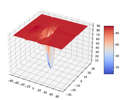
(a) error surface (supervised). left: R-20$\times$4, 94.07%; right: R-20$\times$4_[1.0,0.5], 93.58%, 93.03%.

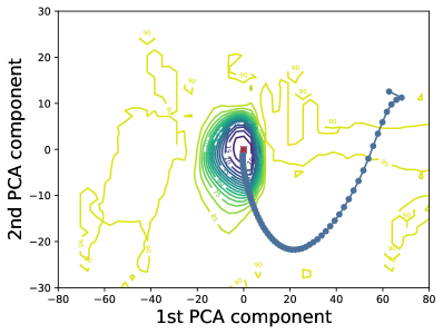
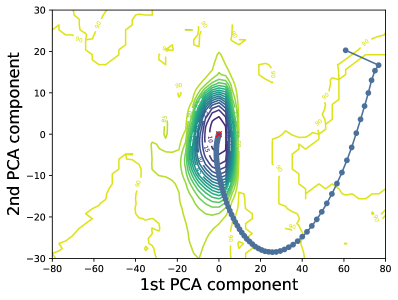
(b) trajectory (supervised). left: R-20$\times$4, 94.07%; right: R-20$\times$4_[1.0,0.5], 93.58%, 93.03%.

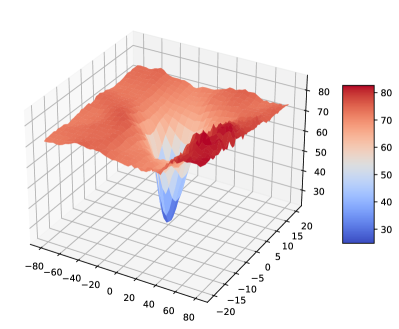
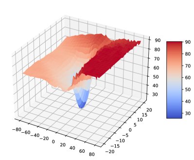
(c) error surface (MoCo). left: R-20$\times$4, 76.75%; right: R-20$\times$4_[1.0,0.5], 75.74%, 74.24%.

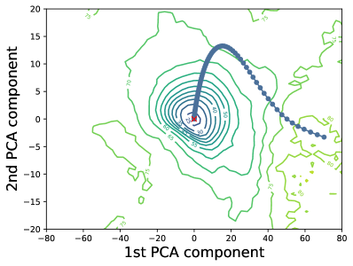
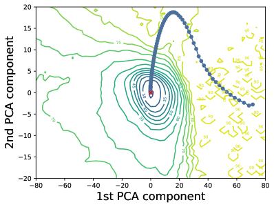
(d) trajectory (MoCo). left: R-20$\times$4, 76.75%; right: R-20$\times$4_[1.0,0.5], 75.74%, 74.24%.

Figure 5: Error surface and optimization trajectory. Best viewed in color with 300% zoom.

Self-supervised and supervised slimmable networks  Training slimmable networks is generally more challenging in self-supervised learning than in supervised learning. In Figure 3 and Figure 4, gradient imbalance and gradient direction divergence are more pronounced in self-supervised cases, leading to more severe performance degradation in Figure 1. To gain a deeper understanding of the difficulty in training slimmable networks in self-supervised learning, we visualize the error surface and optimization trajectory (Li et al., 2018) of slimmable networks during training. Specifically, we train slimmable networks in both supervised and self-supervised (MoCo He et al. (2020)) manners on CIFAR- 10 (Krizhevsky and Hinton, 2009) for 100 epochs, with a ResNet-20$\times$4 base network containing 4.3M parameters. In self-supervised cases, we use a $k$-NN predictor (Wu et al., 2018) to obtain the accuracy. After training, we visualize the error surface and optimization trajectory in Figure 5 following Li et al. (2018).

The visualizations reveal that self-supervised learning is more challenging than supervised learning. In the left error surface of Figure 5(a) and Figure 5(c), it can be observed that the terrain surrounding the valley is relatively flat in supervised cases, while it is more complex in self-supervised cases. Moreover, from the trajectory in the left of Figure 5(b) and Figure 5(d), the contours in supervised cases are denser, indicating that the model in self-supervised cases requires more time to achieve the same accuracy improvement compared to the model in supervised cases.

The visualization indicates that weight-sharing networks have a greater impact in self-supervised cases. Firstly, weight-sharing networks induce significant changes to the error surface in Figure 5(c), while the change is less apparent in supervised cases. Secondly, in self-supervised cases, interference between weight- sharing networks causes the model to deviate further from the global minima (i.e., the origin in the visualization) as illustrated in Figure 5(d). In Figure 5(b), the maximal offsets from the global minima along the 2nd PCA component are 21.75 and 28.49 for ResNet-20$\times$4 and ResNet-20$\times$4_[1.0,0.5], respectively. This represents a 31.0% increase in offset. Conversely, for self-supervised cases in Figure 5(d), the maximal offsets from the global minima along the 2nd PCA component are 13.26 and 18.75 for ResNet-20$\times$4 and ResNet- 20$\times$4_[1.0,0.5], respectively. This increase in offset is 41.4%. Therefore, it is evident that weight-sharing networks have a more pronounced impact in self-supervised cases.

5 Conclusion

In this work, we adapt slimmable networks for contrastive learning to obtain pre-trained small models in a self-supervised manner. By using slimmable networks, we can pre-train once and obtain several models of varying sizes, making them suitable for use across different devices. Additionally, our approach does not require the additional training process of large teacher models, as seen in previous distillation-based methods. However, weight-sharing networks in a slimmable network cause interference during self-supervised learning, resulting in gradient magnitude imbalance and gradient direction divergence. We develop several techniques to relieve the interference among networks during pre-training and linear evaluation. Two specific algorithms are instantiated in this work, i.e., SlimCLR-MoCov2 and SlimCLR-MoCov3. We take extensive experiments on ImageNet and achieve better performance than previous arts with fewer network parameters and FLOPs.

Conflict of interest

The authors declare that they have no conflict of interest.

Data availability

The datasets analysed during the current study are available in https://www.image-net.org/, https://www.cs.toronto.edu/~kriz/cifar.html, and https://cocodataset.org/. No new datasets were generated.

Appendix

Appendix A Conditions of inputs

We consider the conditions of inputs when only using one slimmable linear layer during evaluation, i.e., consider solving multiple multi-class linear regression problems with shared weights. The parameters of the linear layer are $\bm{\theta}\in\mathbb{R}^{d\times C}$, $C$ is the number of classes, where $\bm{\theta}=\begin{bmatrix}\bm{\theta}_{11}\\ \bm{\theta}_{21}\end{bmatrix}$, $\bm{\theta}_{11}\in\mathbb{R}^{d_{1}\times C}$, $\bm{\theta}_{21}\in\mathbb{R}^{d_{2}\times C}$, $d_{1}\ +\ d_{2}\ =\ d$. The first input for the full model is $\bm{X}\in\mathbb{R}^{N\times d}$, where $N$ is the number of samples, ${\bm{X}}=\begin{bmatrix}\bm{X}_{11}&\bm{X}_{12}\end{bmatrix}$, $\bm{X}_{11}\in\mathbb{R}^{N\times d_{1}}$, $\bm{X}_{12}\ \in\mathbb{R}^{N\times d_{2}}$. The second input $\bm{X}_{1}\in\mathbb{R}^{N\times d_{1}}$ is the input feature for the sub-model parameterized by $\bm{\theta}_{11}$. Generally, we have $N\geq d>d_{1}$. We assume that both $\bm{X}$ and $\bm{X}_{1}$ have independent columns, i.e., $\bm{X}^{T}\bm{X}$ and $\bm{X}_{1}^{T}\bm{X}_{1}$ are invertible. The ground truth is $\bm{T}\in\mathbb{R}^{N\times C}$. The prediction of the full model is $\bm{Y}=\bm{X}\bm{\theta}$, to minimize the sum-of-least-squares loss between prediction and ground truth, we get

$$\bm{\theta}=\operatorname*{arg\,min}_{\bm{\theta}}\lVert\bm{X\theta}\ -\ \bm{T}\rVert_{2}^{2}.$$ (8)

By setting the derivative w.r.t. $\bm{\theta}$ to 0, we get

$$\bm{\theta}=\left(\bm{X}^{T}\bm{X}\right)^{-1}\bm{X}^{T}\bm{T}.$$ (9)

In the same way, we can get

$$\bm{\theta}_{11}=\left(\bm{X}_{1}^{T}\bm{X}_{1}\right)^{-1}\bm{X}_{1}^{T}\bm{T}.$$ (10)

For $\bm{X}^{T}\bm{X}$, we have

$$\bm{X}^{T}\bm{X}=\begin{bmatrix}\bm{X}_{11}^{T}\bm{X}_{11}&\bm{X}_{11}^{T}\bm{X}_{12}\\ \bm{X}_{12}^{T}\bm{X}_{11}&\bm{X}_{12}^{T}\bm{X}_{12}\end{bmatrix}.$$ (11)

We denote the inverse of $\bm{X}^{T}\bm{X}$ as $\bm{B}=\begin{bmatrix}\bm{B}_{11}&\bm{B}_{12}\\ \bm{B}_{21}&\bm{B}_{22}\end{bmatrix}$, where $\bm{B}_{12}=\bm{B}_{21}^{T}$ as $\bm{X}^{T}\bm{X}$ is a symmetric matrix. For $\bm{X}^{T}\bm{XB}=\bm{I}$, we have

$$\bm{X}^{T}\bm{X}\begin{bmatrix}\bm{B}_{11}&\bm{B}_{12}\\ \bm{B}_{21}&\bm{B}_{22}\end{bmatrix}=\begin{bmatrix}\bm{I}_{d_{1}}&\bm{0}_{d_{1},\ d_{2}}\\ \bm{0}_{d_{2},\ d_{1}}&\bm{I}_{d_{2}}\end{bmatrix}.$$ (12)

Then we can get

$$\bm{X}_{11}^{T}\bm{X}_{11}\bm{B}_{11}+\bm{X}_{11}^{T}\bm{X}_{12}\bm{B}_{21} =\bm{I}_{d_{1}},$$ (13)

$$\bm{X}_{11}^{T}\bm{X}_{11}\bm{B}_{12}+\bm{X}_{11}^{T}\bm{X}_{12}\bm{B}_{22} =\bm{0}_{d_{1},\ d_{2}},$$ (14)

$$\bm{X}_{12}^{T}\bm{X}_{11}\bm{B}_{11}+\bm{X}_{12}^{T}\bm{X}_{12}\bm{B}_{21} =\bm{0}_{d_{1},\ d_{2}},$$ (15)

$$\bm{X}_{12}^{T}\bm{X}_{11}\bm{B}_{12}+\bm{X}_{12}^{T}\bm{X}_{12}\bm{B}_{22} =\bm{I}_{d_{2}}.$$ (16)

At the same time

$$\bm{\theta} =\left(\bm{X}^{T}\bm{X}\right)^{-1}\bm{X}^{T}\bm{T}=\bm{BX}^{T}\bm{T}$$

$$=\begin{bmatrix}\bm{B}_{11}&\bm{B}_{12}\\ \bm{B}_{21}&\bm{B}_{22}\end{bmatrix}\begin{bmatrix}\bm{X}_{11}&\bm{X}_{12}\end{bmatrix}^{T}\bm{T}$$

$$=\begin{bmatrix}\bm{B}_{11}\bm{X}_{11}^{T}+\bm{B}_{12}\bm{X}_{12}^{T}\\ \bm{B}_{21}\bm{X}_{11}^{T}+\bm{B}_{22}\bm{X}_{12}^{T}\end{bmatrix}\bm{T},$$ (17)

and

$$\bm{\theta}_{11}\ =\ \left(\bm{B}_{11}\bm{X}_{11}^{T}+\bm{B}_{12}\bm{X}_{12}^{T}\right)\bm{T}$$

$$=\left(\bm{X}_{1}^{T}\bm{X}_{1}\right)^{-1}\bm{X}_{1}^{T}\bm{T}.$$ (18)

From Eq. (15), we get

$$\bm{B}_{21} =-\left(\bm{X}_{12}^{T}\bm{X}_{12}\right)^{-1}\bm{X}_{12}^{T}\bm{X}_{11}\bm{B}_{11},$$ (19)

$$\bm{B}_{12} =\bm{-B}_{11}\bm{X}_{11}^{T}\bm{X}_{12}\left(\bm{X}_{12}^{T}\bm{X}_{12}\right)^{-1}.$$ (20)

Substitute Eq. (19) into Eq. (13), we get

$$\bm{B}_{11}\ =$$

$$\left(\ \bm{X}_{11}^{T}\bm{X}_{11}-\bm{X}_{11}^{T}\bm{X}_{12}\left(\bm{X}_{12}^{T}\bm{X}_{12}\right)^{-1}\bm{X}_{12}^{T}\bm{X}_{11}\right)^{-1}.$$ (21)

At the same time

$$\bm{\theta}_{11} =\left(\bm{B}_{11}\bm{X}_{11}^{T}+\bm{B}_{12}\bm{X}_{12}^{T}\right)\bm{T}$$

$$=\bm{B}_{11}\left(\bm{X}_{11}^{T}-\bm{X}_{11}^{T}\bm{X}_{12}\left(\bm{X}_{12}^{T}\bm{X}_{12}\right)^{-1}\bm{X}_{12}^{T}\right)\bm{T}.$$ (22)

Combining Eq. (A) and Eq. (A), we get the condition of the input

$$\bm{B}_{11}\left(\bm{X}_{11}^{T}-\bm{X}_{11}^{T}\bm{X}_{12}\left(\bm{X}_{12}^{T}\bm{X}_{12}\right)^{-1}\bm{X}_{12}^{T}\right)\bm{T}=$$

$$\left(\bm{X}_{1}^{T}\bm{X}_{1}\right)^{-1}\bm{X}_{1}^{T}\bm{T}.$$ (23)

In order to verify whether the input condition in Eq. (A) is met in practice, we randomly sampled 2048 images from the training set of ImageNet and used a ResNet-50_{[1.0,0.75,0.5,0.25]} pre- trained by SlimCLR-MoCov2 (800 epochs) to extract their features. The features extracted by ResNet-50_1.0 are denoted as $\bm{X}\in\mathbb{R}^{2048\times 1024}$, and the features extracted by ResNet-50_0.5 are denoted as $\bm{X}_{1}\in\mathbb{R}^{2048\times 512}$. We use $\bm{L}$ to represent the left side of Eq. (A) and $\bm{R}$ for the right side. Then, we calculate the absolute difference between $\bm{L}$ and $\bm{R}$, denoted as $\lvert\bm{L}-\bm{R}\rvert$. The average value of entries in $\lvert\bm{L}-\bm{R}\rvert$ is $1.07$, which indicates a total difference of $1096665.50$. We also conducted similar experiments on the validation set of ImageNet and found that the average value of entries in $\lvert\bm{L}-\bm{R}\rvert$ is $0.88$, which indicates a total difference of $903094.19$.

These results demonstrate that the features of a slimmable network learned by contrastive self-supervised learning cannot meet the input conditions in Eq. (A) when using a single slimmable linear probe layer. This provides an explanation for why using a switchable linear probe layer achieves much better performance in Table 3(a).

References

- Bachman et al. (2019) Bachman P, Hjelm RD, Buchwalter W (2019) Learning representations by maximizing mutual information across views. In: NeurIPS
- Ballard (1987) Ballard DH (1987) Modular learning in neural networks. In: AAAI
- Cai et al. (2020) Cai H, Gan C, Wang T, Zhang Z, Han S (2020) Once-for-all: Train one network and specialize it for efficient deployment. In: ICLR
- Caron et al. (2018) Caron M, Bojanowski P, Joulin A, Douze M (2018) Deep clustering for unsupervised learning of visual features. In: ECCV
- Chavan et al. (2022) Chavan A, Shen Z, Liu Z, Liu Z, Cheng KT, Xing EP (2022) Vision transformer slimming: Multi-dimension searching in continuous optimization space. In: CVPR
- Chen et al. (2019) Chen K, Wang J, Pang J, Cao Y, Xiong Y, Li X, Sun S, Feng W, Liu Z, Xu J, Zhang Z, Cheng D, Zhu C, Cheng T, Zhao Q, Li B, Lu X, Zhu R, Wu Y, Dai J, Wang J, Shi J, Ouyang W, Loy CC, Lin D (2019) MMDetection: Open mmlab detection toolbox and benchmark. arXiv preprint arXiv:190607155
- Chen et al. (2020a) Chen T, Kornblith S, Norouzi M, Hinton GE (2020a) A simple framework for contrastive learning of visual representations. In: ICML
- Chen et al. (2020b) Chen T, Kornblith S, Swersky K, Norouzi M, Hinton GE (2020b) Big self-supervised models are strong semi-supervised learners. In: NeurIPS
- Chen and He (2021) Chen X, He K (2021) Exploring simple siamese representation learning. In: CVPR
- Chen et al. (2020c) Chen X, Fan H, Girshick RB, He K (2020c) Improved baselines with momentum contrastive learning. CoRR abs/2003.04297, 2003.04297
- Chen et al. (2021) Chen X, Xie S, He K (2021) An empirical study of training self-supervised vision transformers. In: ICCV
- Devlin et al. (2019) Devlin J, Chang M, Lee K, Toutanova K (2019) BERT: pre-training of deep bidirectional transformers for language understanding. In: NAACL-HLT
- Dosovitskiy et al. (2016) Dosovitskiy A, Fischer P, Springenberg JT, Riedmiller MA, Brox T (2016) Discriminative unsupervised feature learning with exemplar convolutional neural networks. TPAMI
- Fang et al. (2021) Fang Z, Wang J, Wang L, Zhang L, Yang Y, Liu Z (2021) SEED: self-supervised distillation for visual representation. In: ICLR
- Gao et al. (2022) Gao Y, Zhuang J, Lin S, Cheng H, Sun X, Li K, Shen C (2022) Disco: Remedy self-supervised learning on lightweight models with distilled contrastive learning. In: ECCV
- Goyal et al. (2017) Goyal P, Dollár P, Girshick RB, Noordhuis P, Wesolowski L, Kyrola A, Tulloch A, Jia Y, He K (2017) Accurate, large minibatch SGD: training imagenet in 1 hour. CoRR abs/1706.02677, 1706.02677
- Guo (2022) Guo J (2022) Reducing the teacher-student gap via adaptive temperatures
- He et al. (2016) He K, Zhang X, Ren S, Sun J (2016) Deep residual learning for image recognition. In: CVPR
- He et al. (2017) He K, Gkioxari G, Dollár P, Girshick RB (2017) Mask R-CNN. In: ICCV, pp 2980–2988
- He et al. (2020) He K, Fan H, Wu Y, Xie S, Girshick RB (2020) Momentum contrast for unsupervised visual representation learning. In: CVPR
- He et al. (2022) He K, Chen X, Xie S, Li Y, Dollár P, Girshick R (2022) Masked autoencoders are scalable vision learners. In: CVPR
- He et al. (2019) He T, Zhang Z, Zhang H, Zhang Z, Xie J, Li M (2019) Bag of tricks for image classification with convolutional neural networks. In: CVPR
- Hinton et al. (2015) Hinton GE, Vinyals O, Dean J (2015) Distilling the knowledge in a neural network. CoRR abs/1503.02531
- Hjelm et al. (2019) Hjelm RD, Fedorov A, Lavoie-Marchildon S, Grewal K, Bachman P, Trischler A, Bengio Y (2019) Learning deep representations by mutual information estimation and maximization. In: ICLR
- Ioffe and Szegedy (2015) Ioffe S, Szegedy C (2015) Batch normalization: Accelerating deep network training by reducing internal covariate shift. In: ICML
- Kingma and Welling (2014) Kingma DP, Welling M (2014) Auto-encoding variational bayes. In: ICLR
- Koohpayegani et al. (2020) Koohpayegani SA, Tejankar A, Pirsiavash H (2020) Compress: Self-supervised learning by compressing representations. In: NeurIPS
- Krizhevsky and Hinton (2009) Krizhevsky A, Hinton G (2009) Learning multiple layers of features from tiny images. Technical report, University of Toronto
- Li et al. (2021) Li C, Wang G, Wang B, Liang X, Li Z, Chang X (2021) Dynamic slimmable network. In: CVPR
- Li et al. (2022) Li C, Wang G, Wang B, Liang X, Li Z, Chang X (2022) Ds-net++: Dynamic weight slicing for efficient inference in cnns and transformers. T-PAMI
- Li et al. (2018) Li H, Xu Z, Taylor G, Studer C, Goldstein T (2018) Visualizing the loss landscape of neural nets. In: NeurIPS
- Lin et al. (2014) Lin T, Maire M, Belongie SJ, Hays J, Perona P, Ramanan D, Dollár P, Zitnick CL (2014) Microsoft COCO: common objects in context. In: ECCV
- Lin et al. (2017) Lin T, Dollár P, Girshick RB, He K, Hariharan B, Belongie SJ (2017) Feature pyramid networks for object detection. In: CVPR, pp 936–944
- Liu et al. (2020) Liu X, Zhang F, Hou Z, Wang Z, Mian L, Zhang J, Tang J (2020) Self-supervised learning: Generative or contrastive. CoRR abs/2006.08218
- Liu et al. (2017) Liu Z, Li J, Shen Z, Huang G, Yan S, Zhang C (2017) Learning efficient convolutional networks through network slimming. In: ICCV
- Micikevicius et al. (2018) Micikevicius P, Narang S, Alben J, Diamos GF, Elsen E, García D, Ginsburg B, Houston M, Kuchaiev O, Venkatesh G, Wu H (2018) Mixed precision training. In: ICLR
- Mirzadeh et al. (2020) Mirzadeh S, Farajtabar M, Li A, Levine N, Matsukawa A, Ghasemzadeh H (2020) Improved knowledge distillation via teacher assistant. In: AAAI
- van den Oord et al. (2016a) van den Oord A, Kalchbrenner N, Espeholt L, Kavukcuoglu K, Vinyals O, Graves A (2016a) Conditional image generation with pixelcnn decoders. In: NeurIPS
- van den Oord et al. (2016b) van den Oord A, Kalchbrenner N, Kavukcuoglu K (2016b) Pixel recurrent neural networks. In: ICML
- van den Oord et al. (2018) van den Oord A, Li Y, Vinyals O (2018) Representation learning with contrastive predictive coding. CoRR abs/1807.03748
- Park et al. (2019) Park W, Kim D, Lu Y, Cho M (2019) Relational knowledge distillation. In: CVPR, DOI 10.1109/CVPR.2019.00409
- Pathak et al. (2016) Pathak D, Krähenbühl P, Donahue J, Darrell T, Efros AA (2016) Context encoders: Feature learning by inpainting. In: CVPR
- Peng et al. (2019) Peng B, Jin X, Li D, Zhou S, Wu Y, Liu J, Zhang Z, Liu Y (2019) Correlation congruence for knowledge distillation. In: ICCV, DOI 10.1109/ICCV.2019.00511
- Radford et al. (2016) Radford A, Metz L, Chintala S (2016) Unsupervised representation learning with deep convolutional generative adversarial networks. In: ICLR
- Russakovsky et al. (2015) Russakovsky O, Deng J, Su H, Krause J, Satheesh S, Ma S, Huang Z, Karpathy A, Khosla A, Bernstein MS, Berg AC, Li F (2015) Imagenet large scale visual recognition challenge. IJCV
- Tian et al. (2020) Tian Y, Krishnan D, Isola P (2020) Contrastive representation distillation. In: ICLR
- Tomasev et al. (2022) Tomasev N, Bica I, McWilliams B, Buesing L, Pascanu R, Blundell C, Mitrovic J (2022) Pushing the limits of self-supervised resnets: Can we outperform supervised learning without labels on imagenet? CoRR abs/2201.05119
- Wang et al. (2021) Wang W, Chen M, Zhao S, Chen L, Hu J, Liu H, Cai D, He X, Liu W (2021) Accelerate cnns from three dimensions: A comprehensive pruning framework. In: ICML
- Wu et al. (2018) Wu Z, Xiong Y, Yu SX, Lin D (2018) Unsupervised feature learning via non-parametric instance discrimination. In: CVPR
- Xu et al. (2022) Xu H, Fang J, Zhang X, Xie L, Wang X, Dai W, Xiong H, Tian Q (2022) Bag of instances aggregation boosts self-supervised distillation. In: ICLR
- Yang et al. (2020) Yang T, Zhu S, Chen C, Yan S, Zhang M, Willis AR (2020) Mutualnet: Adaptive convnet via mutual learning from network width and resolution. In: ECCV
- You et al. (2017) You Y, Gitman I, Ginsburg B (2017) Large batch training of convolutional networks. arXiv preprint arXiv:170803888
- Yu and Huang (2019a) Yu J, Huang T (2019a) Autoslim: Towards one-shot architecture search for channel numbers. arXiv preprint arXiv:190311728
- Yu and Huang (2019b) Yu J, Huang TS (2019b) Universally slimmable networks and improved training techniques. In: ICCV
- Yu et al. (2019) Yu J, Yang L, Xu N, Yang J, Huang TS (2019) Slimmable neural networks. In: ICLR
- Yu et al. (2020) Yu J, Jin P, Liu H, Bender G, Kindermans P, Tan M, Huang TS, Song X, Pang R, Le Q (2020) Bignas: Scaling up neural architecture search with big single-stage models. In: ECCV, Springer, pp 702–717
- Zhang et al. (2016) Zhang R, Isola P, Efros AA (2016) Colorful image colorization. In: ECCV
- Zhang et al. (2018) Zhang Y, Xiang T, Hospedales TM, Lu H (2018) Deep mutual learning. In: CVPR, DOI 10.1109/CVPR.2018.00454
- Zhao et al. (2022a) Zhao B, Cui Q, Song R, Qiu Y, Liang J (2022a) Decoupled knowledge distillation. In: CVPR
- Zhao et al. (2022b) Zhao S, Zhou L, Wang W, Cai D, Lam TL, Xu Y (2022b) Towards better accuracy-efficiency trade-offs: Divide and co-training. TIP