Realizing efficient quantum error-correction with three-qubit codes

Abstract

In this work, the efficient quantum error-correction protocol against the general independent noise is constructed with the three-qubit quantum error-correction codes. The rules of concatenation are summarized according to the error-correcting capability of the codes. The codes not only play the role of correcting errors, but the role of polarizing the effective channel. The performance of the protocol is dependent on the type of noise and the level of concatenation. For the general Pauli noise, the threshold of the protocol is $0.91518$ when against the depolarizing noise, while for the amplitude damping noise it is about $0.849$. For the general independent noise, the threshold of the protocol is about $0.932$, which is obtained through the numerical simulations. If there is no limit on the level of concatenation, the error-correction threshold can be much lower. The physical resources costed by this protocol is multiple of the physical resources costed by realizing the three-qubit quantum error-correction, with no increase in complexity. We believe it will be helpful for realizing quantum error-correction in the physical system.

Introduction.—In quantum computation and communication, quantum error-correction (QEC) developed from classic schemes to preserving coherent states from noise and other unexpected interactions. It was independently discovered by Shor and Steane Shor ; Steane . The QEC conditions were proved independently by Bennett, DiVincenzo, Smolin and Wootters Bennett , and by Knill and Laflamme Knill . QEC codes are introduced as active error-correction. The nine-qubit code was discovered by Shor, called the Shor code. The seven-qubit code was discovered by Steane, called the Steane code. The five-qubit code was discovered by Bennett, DiVincenzo, Smolin and Wootters Bennett , and independently by Laflamme, Miquel, Paz and Zurek Laflamme .

There are many constructions for specific classes of quantum codes. Rains, Hardin, Shor and Sloane Rains have constructed interesting examples of quantum codes lying outside the stabilizer codes. Gottesman Gottesman2 and Rains Rains2 construct non-binary codes and consider fault-tolerant computation with such codes. Aharonov and Ben-Or Aharonov construct non-binary codes using interesting techniques based on polynomials over finite fields, and also investigate fault-tolerant computation with such codes. Approximate QEC can lead to improved codes was shown by Leung, Nielsen, Chuang and Yamamoto Leung .

Calderbank and Shor Calderbank , and Steane Steane2 used ideas from classical error-correction to develop the CSS (Calderbank-Shor-Steane) codes. Calderbank and Shor also stated and proved the Gilbert-Varshamov bound for CSS codes. Gottesman Gottesman invented the stabilizer formalism, and used it to define stabilizer codes, and investigated some of the properties of some specific codes. Independently, Calderbank, Rains, Shor and Sloane Calderbank2 invented an essentially equivalent approach to QEC based on ideas from classical coding theory.

QEC codes are introduced as active error-correction. Another way, passive error-avoiding techniques contain decoherence-free subspaces Duan ; Lidar ; Zanardi and noiseless subsystem KandLV ; Zanardi2 ; Kempe . Recently, it has been proven that both the active and passive QEC methods can be unified Kribs ; Poulin 05 ; Kribs2 . So, more QEC codes means more options for suppressing noise, and more options for optimizing the performance of QEC. Meanwhile, how to realize efficient QEC with these codes in the physical system is still an important question.

As known, the three-qubit code is not efficient for arbitrary one-qubit errors because of the Hamming bound. We still used it for QEC simulation because it is the simplest QEC code. The three-qubit code is bound to cause channel fidelity to improve when the weight of the polarizing error (Pauli-X, Y, or Z) is above $\frac{2}{3}$. The three-qubit code in Eq. (Realizing efficient quantum error-correction with three-qubit codes) will change the polarizing of the effective channel to Pauli-Z after QEC, and the three-qubit code in Eq. (Realizing efficient quantum error-correction with three-qubit codes) will change the polarizing of the effective channel to Pauli-X after QEC. Based on the reasons, under certain conditions, the QEC for arbitrary one-qubit errors can be realized in nine-qubit channels when the two three-qubit codes are applied in concatenated. Meanwhile, we should notice that correcting arbitrary one-qubit errors is an equivalent description for the performance of QEC, which means the channel fidelity of the effective channel is no less than $f_{0}^{9}+9f_{0}^{8}(1-f_{0})$. Here, $f_{0}$ is the channel fidelity of the initial channel, and $1-f_{0}$ is the possibility of all errors in the initial channel.

In this work, the efficient quantum error-correction protocol against the general independent noise is constructed with the three-qubit quantum error-correction codes. The rules of concatenation are summarized according to the error-correcting capability of the codes. The codes not only play the role of correcting errors, but the role of polarizing the effective channel. The performance of the protocol is dependent on the type of noise and the level of concatenation.

Three-qubit codes.—In the first place, we introduce the two simplest three-qubit QEC codes Fig. (1), because only the two simplest three-qubit codes can be used for encoding the physical qubits. One is the bit-flip code, which is the simplest code with the stabilizer $\langle Z_{1}Z_{2},Z_{2}Z_{3}\rangle$,

$$|0_{\mathcal{L}}\rangle=|000\rangle,$$

$$|1_{\mathcal{L}}\rangle=|111\rangle.$$ (1)

With the code, the state $|\psi\rangle=a|0\rangle+b|1\rangle$ is encoded to $|\tilde{\psi}\rangle=a|000\rangle+b|111\rangle$. For the code in Eq. (Realizing efficient quantum error-correction with three-qubit codes), the correctable errors are $X_{1},X_{2},X_{3}$, $Z_{1}Z_{2},Z_{1}Z_{3},Z_{2}Z_{3}$, $Y_{1}Z_{2},Y_{1}Z_{3},Y_{2}Z_{3}$, $Z_{1}Y_{2},Z_{1}Y_{3},Z_{2}Y_{3}$, and $Z_{1}Z_{2}X_{3},Z_{1}Z_{3}X_{2},Z_{2}Z_{3}X_{1}$ (for Pauli-Y errors, the correctable errors are replacing the $X$ as $Y$, and the $Y$ as $X$). Because the list of correctable errors result in the same states as $X_{1},X_{2},X_{3}$, which are identifiable and correctable,

$$X_{1}|\tilde{\psi}\rangle = a|100\rangle+b|011\rangle,$$

$$X_{2}|\tilde{\psi}\rangle = a|010\rangle+b|101\rangle,$$

$$X_{3}|\tilde{\psi}\rangle = a|001\rangle+b|110\rangle.$$

For Pauli-Y errors, the list of correctable errors result in the same states as $Y_{1},Y_{2},Y_{3}$, which are identifiable and correctable,

$$Y_{1}|\tilde{\psi}\rangle = i[a|100\rangle-b|011\rangle],$$

$$Y_{2}|\tilde{\psi}\rangle = i[a|010\rangle-b|101\rangle],$$

$$Y_{3}|\tilde{\psi}\rangle = i[a|001\rangle-b|110\rangle].$$

The other is the phase-flip code, which is the simplest code with the stabilizer $\langle X_{1}X_{2},X_{2}X_{3}\rangle$,

$$|0_{\mathcal{L}}\rangle=\frac{1}{2}[|000\rangle+|011\rangle+|101\rangle+|110\rangle],$$

$$|1_{\mathcal{L}}\rangle=\frac{1}{2}[|111\rangle+|100\rangle+|010\rangle+|001\rangle].$$ (2)

With the code, the state $|\psi\rangle=a|0\rangle+b|1\rangle$ is encoded to $|\tilde{\psi}\rangle=a[|000\rangle+|011\rangle+|101\rangle+|110\rangle]+b[|111\rangle+|100\rangle+|010\rangle+|001\rangle]$. For the code in Eq. (Realizing efficient quantum error-correction with three-qubit codes), the correctable errors are $Z_{1},Z_{2},Z_{3}$, $X_{1}X_{2},X_{1}X_{3},X_{2}X_{3}$, $Y_{1}X_{2},Y_{1}X_{3},Y_{2}X_{3}$, $X_{1}Y_{2},X_{1}Y_{3},X_{2}Y_{3}$, and $X_{1}X_{2}Z_{3},X_{1}X_{3}Z_{2},X_{2}X_{3}Z_{1}$ (for Pauli-Y errors, the correctable errors are replacing the $Z$ as $Y$, and the $Y$ as $Z$). Because the list of correctable errors result in the same states as $Z_{1},Z_{2},Z_{3}$, which are identifiable and correctable,

$$Z_{1}|\tilde{\psi}\rangle = a[|000\rangle+|011\rangle-|101\rangle-|110\rangle]$$

$$+b[-|111\rangle-|100\rangle+|010\rangle+|001\rangle],$$

$$Z_{2}|\tilde{\psi}\rangle = a[|000\rangle-|011\rangle+|101\rangle-|110\rangle]$$

$$+b[-|111\rangle+|100\rangle-|010\rangle+|001\rangle],$$

$$Z_{3}|\tilde{\psi}\rangle = a[|000\rangle-|011\rangle-|101\rangle+|110\rangle]$$

$$+b[-|111\rangle+|100\rangle+|010\rangle-|001\rangle].$$

For Pauli-Y errors, the list of correctable errors result in the same states as $Y_{1},Y_{2},Y_{3}$, which are identifiable and correctable,

$$Y_{1}|\tilde{\psi}\rangle = i[a[|100\rangle+|111\rangle-|001\rangle-|010\rangle]$$

$$+b[-|011\rangle-|000\rangle+|110\rangle+|101\rangle]],$$

$$Y_{2}|\tilde{\psi}\rangle = i[a[|010\rangle-|001\rangle+|111\rangle-|100\rangle]$$

$$+b[-|101\rangle+|110\rangle-|000\rangle+|011\rangle]],$$

$$Y_{3}|\tilde{\psi}\rangle = i[a[|001\rangle-|010\rangle-|100\rangle+|111\rangle]$$

$$+b[-|110\rangle+|101\rangle+|011\rangle-|000\rangle]].$$

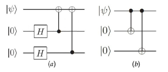
Figure 1: (a) Encoding circuits for the phase-flip code. (b) Encoding circuits for the bit-flip code.

Then, we introduce other two three-qubit QEC codes, which can not be used for encoding the physical qubits, but the QEC protocol may be simplified with them. When they are used for encoding the physical qubits, efficient error correction can not be realized because the logical code words will be degenerate. One is obtained by applying the logical $H$ on the code in Eq. (Realizing efficient quantum error-correction with three-qubit codes),

$$|0_{\mathcal{L}}\rangle=\frac{1}{\sqrt{2}}[|000\rangle+|111\rangle],$$

$$|1_{\mathcal{L}}\rangle=\frac{1}{\sqrt{2}}[|000\rangle-|111\rangle].$$ (3)

The other is obtained by applying the logical $H$ on the code in Eq. (Realizing efficient quantum error-correction with three-qubit codes),

$$|0_{\mathcal{L}}\rangle = \frac{1}{2\sqrt{2}}[|000\rangle+|011\rangle+|101\rangle+|110\rangle$$

$$+|111\rangle+|100\rangle+|010\rangle+|001\rangle],$$

$$|1_{\mathcal{L}}\rangle = \frac{1}{2\sqrt{2}}[|000\rangle+|011\rangle+|101\rangle+|110\rangle$$ (4)

$$-|111\rangle-|100\rangle-|010\rangle-|001\rangle].$$

Performance for the general Pauli noise.—The general Pauli noise is represented by $\varepsilon_{0}$,

$$\varepsilon_{0}=f_{0}\hat{\sigma}_{I}+p_{x}\hat{\sigma}_{x}+p_{y}\hat{\sigma}_{y}+p_{z}\hat{\sigma}_{z}.$$

Here, $f_{0}$ is the channel fidelity, and $p_{x},p_{y},p_{z}$ is the probability of the Pauli-X, Pauli-Y, Pauli-Z, respectively. There are four different schemes for the general Pauli noise when it is the physical noise, and only the codes in Eq. (Realizing efficient quantum error-correction with three-qubit codes) and Eq. (Realizing efficient quantum error-correction with three-qubit codes) are available. The effective channel can be represented by $\varepsilon_{1}$ after one-level QEC.

For the code in Eq. (Realizing efficient quantum error-correction with three-qubit codes), when correcting $X_{1},X_{2},X_{3}$,

$$f_{1} = f_{0}^{3}+3f_{0}^{2}p_{x}+3f_{0}p_{z}^{2}+6f_{0}p_{y}p_{z}+3p_{x}p_{z}^{2}$$

$$p1_{z} = p_{z}^{3}+3p_{z}^{2}p_{y}+3p_{z}f_{0}^{2}+6f_{0}p_{x}p_{z}+3p_{y}f_{0}^{2}$$

$$p1_{x} = p_{x}^{3}+3p_{x}^{2}f_{0}+3p_{x}p_{y}^{2}+6p_{x}p_{y}p_{z}+3f_{0}p_{y}^{2}$$

$$p1_{y} = p_{y}^{3}+3p_{y}^{2}p_{z}+3p_{y}p_{x}^{2}+6f_{0}p_{y}p_{x}+3p_{z}p_{x}^{2}.$$ (5)

When correcting $Y_{1},Y_{2},Y_{3}$, the results can be obtained by replacing the $p_{x}$ with $p_{y}$, and the $p_{y}$ with $p_{x}$ in Eq. (Realizing efficient quantum error-correction with three-qubit codes).

For the code in Eq. (Realizing efficient quantum error-correction with three-qubit codes), when correcting $Z_{1},Z_{2},Z_{3}$,

$$f_{1} = f_{0}^{3}+3f_{0}^{2}p_{z}+3f_{0}p_{x}^{2}+6f_{0}p_{y}p_{x}+3p_{z}p_{x}^{2}$$

$$p1_{z} = p_{z}^{3}+3p_{z}^{2}f_{0}+3p_{z}p_{y}^{2}+6p_{z}p_{x}p_{y}+3f_{0}p_{y}^{2}$$

$$p1_{x} = p_{x}^{3}+3p_{x}^{2}p_{y}+3p_{x}f_{0}^{2}+6p_{x}p_{z}f_{0}+3p_{y}f_{0}^{2}$$

$$p1_{y} = p_{y}^{3}+3p_{y}^{2}p_{x}+3p_{y}p_{z}^{2}+6p_{y}f_{0}p_{z}+3p_{x}p_{z}^{2}.$$ (6)

When correcting $Y_{1},Y_{2},Y_{3}$, the results can be obtained by replacing the $p_{z}$ with $p_{y}$, and the $p_{y}$ with $p_{z}$ in Eq. (Realizing efficient quantum error-correction with three-qubit codes).

Here, $f_{1}$ is the channel fidelity, and $p1_{x},p1_{y},p1_{z}$ is the probability of the Pauli-X, Pauli-Y, Pauli-Z, respectively. In general cases, $f_{0}\gg p_{x},p_{y},p_{z}$. So, based on the value of $p1_{z}$ in Eq. (Realizing efficient quantum error-correction with three-qubit codes) and $p1_{x}$ in Eq. (Realizing efficient quantum error-correction with three-qubit codes), the three-qubit codes have the ability to polarize the effective channel. The code in Eq. (Realizing efficient quantum error-correction with three-qubit codes) will polarize the effective channel to Pauli-Z, and the code in Eq. (Realizing efficient quantum error-correction with three-qubit codes) will polarize the effective channel to Pauli-X. This phenomenon makes the effective channel more correctable, and increases the possibility of realizing efficient QEC with the three-qubit codes.

Rules of concatenation.—Based on the Eq. (Realizing efficient quantum error-correction with three-qubit codes) and Eq. (Realizing efficient quantum error-correction with three-qubit codes), $4^{8}$ different combinations with the four Pauli operators are correctable when concatenated the two codes in Eq. (Realizing efficient quantum error-correction with three-qubit codes) and Eq. (Realizing efficient quantum error-correction with three-qubit codes). Fortunately, the correctable errors contain all one-wight errors, which is the necessary condition for efficient QEC. Now, the core problem we need to solve becomes how to improve performance under the premise of efficient QEC. There are three rules we should follow,

1. The codes used for encoding the physical qubits must be the simplest three-qubit codes. Otherwise, the logical code words will be degenerate in concatenated QEC.

2. If the Pauli-Y errors need to be corrected, it should be done in the physical qubits. Otherwise, the best performance can not be reached, because the effective channel will be approaching to Pauli-Z or Pauli-X after QEC with any three-qubit code. In the case $p_{y}\leq p_{x},p_{z}$, the Pauli-Y errors can be neglected. In the rest cases, the Pauli-Y errors need to be corrected, and the choice of code depends on the weights of Pauli-X and Pauli-Z. When $p_{z}>p_{x}$, a better performance can be reached with the code in Eq. (Realizing efficient quantum error-correction with three-qubit codes). When $p_{z}<p_{x}$, a better performance can be reached with the code in Eq. (Realizing efficient quantum error-correction with three-qubit codes). When $p_{z}=p_{x}$, the same performance is reached with the codes in Eq. (Realizing efficient quantum error-correction with three-qubit codes) and Eq. (Realizing efficient quantum error-correction with three-qubit codes).

3. In the logical level-l, the choice of code depends on the weights of Pauli-X, Pauli-Y and Pauli-Z. Here, $pl_{x},pl_{y},pl_{z}$ is the probability of the Pauli-X, Pauli-Y, Pauli-Z in concatenated level-$l$, respectively. If $pl_{y}$ is the maximum, the choice of code depends on the values of $pl_{x}$ and $pl_{z}$. When $pl_{z}>pl_{x}$, a better performance can be reached with the code in Eq. (Realizing efficient quantum error-correction with three-qubit codes) or Eq. (Realizing efficient quantum error-correction with three-qubit codes). When $pl_{z}<pl_{x}$, a better performance can be reached with the code in Eq. (Realizing efficient quantum error-correction with three-qubit codes) or Eq. (Realizing efficient quantum error-correction with three-qubit codes). If $pl_{x}$ is the maximum, a better performance can be reached with the code in Eq. (Realizing efficient quantum error-correction with three-qubit codes) or Eq. (Realizing efficient quantum error-correction with three-qubit codes). If $pl_{z}$ is the maximum, a better performance can be reached with the code in Eq. (Realizing efficient quantum error-correction with three-qubit codes) or Eq. (Realizing efficient quantum error-correction with three-qubit codes). Here, we introduce the codes in Eq. (Realizing efficient quantum error-correction with three-qubit codes) and Eq. (Realizing efficient quantum error-correction with three-qubit codes), because they may make the concatenated protocol much simpler. As known from Eq. (Realizing efficient quantum error-correction with three-qubit codes) and Eq. (Realizing efficient quantum error-correction with three-qubit codes), the code in Eq. (Realizing efficient quantum error-correction with three-qubit codes) will polarize the effective channel to Pauli-Z, and the code in Eq. (Realizing efficient quantum error-correction with three-qubit codes) will polarize the effective channel to Pauli-X. When applied logical $H$ on the codes in Eq. (Realizing efficient quantum error-correction with three-qubit codes) and Eq. (Realizing efficient quantum error-correction with three-qubit codes), the code in Eq. (Realizing efficient quantum error-correction with three-qubit codes) will polarize the effective channel to Pauli-X, and the code in Eq. (Realizing efficient quantum error-correction with three-qubit codes) will polarize the effective channel to Pauli-Z. The codes in Eq. (Realizing efficient quantum error-correction with three-qubit codes) and Eq. (Realizing efficient quantum error-correction with three-qubit codes) can be repeated in the logical level of concatenated QEC, usually from the level-2 or level-3.

Examples.—Before applying the concatenated QEC with three-qubit codes, we introduce the representation of the protocol. Written $C_{i}(\hat{\sigma}_{j}),i=1,2,3,4,j=x,y,z$, $C_{i}$ represents which code in Eq. (Realizing efficient quantum error-correction with three-qubit codes) to (Realizing efficient quantum error-correction with three-qubit codes) is applied, and $(\hat{\sigma}_{j})$ represents which errors are corrected with this code.

1. Depolarizing channel. Based on the rules of concatenation, it is depolarizing channel that the worst performance of the protocol against the general Pauli noise. When limit the concatenated level $l=2$, one protocol written as $C_{1}(\hat{\sigma}_{x})C_{2}(\hat{\sigma}_{z})$, and the error-correction threshold is $f_{0}=0.91518$. A much lower error-correction threshold $f_{0}=0.875$ can be reached with no limit on the concatenated level, which is obtained after one 10-level protocol written as $C_{2}(\hat{\sigma}_{z})C_{1}(\hat{\sigma}_{x})C_{3}(\hat{\sigma}_{x})C_{3}(\hat{\sigma}_{x})C_{3}(\hat{\sigma}_{x})C_{3}(\hat{\sigma}_{x})C_{3}(\hat{\sigma}_{x})C_{3}(\hat{\sigma}_{x})\\ C_{4}(\hat{\sigma}_{z})C_{4}(\hat{\sigma}_{z})$ applied. In order to show the evolution of the effective channel, we apply one 10-level protocol written as $C_{1}(\hat{\sigma}_{y})C_{2}(\hat{\sigma}_{z})C_{2}(\hat{\sigma}_{z})C_{1}(\hat{\sigma}_{x})C_{2}(\hat{\sigma}_{z})C_{1}(\hat{\sigma}_{x})C_{2}(\hat{\sigma}_{z})C_{1}(\hat{\sigma}_{x})\\ C_{1}(\hat{\sigma}_{x})C_{2}(\hat{\sigma}_{z})$ on the depolarizing channel with fidelity $0.92$, and the results are obtained in Table 1.

2. Amplitude damping noise. There are two ways to select the optimal QEC protocol for none Pauli noise, one is to treat it as an approximate Pauli channel, and the other is dependent on the performance with all possible QEC protocols. The amplitude damping noise may be treated as one channel, in which $p_{y}>p_{x}>p_{z}$. The QEC protocol should begin with $C_{2}(\hat{\sigma}_{y})C_{1}(\hat{\sigma}_{x})$, and the error-correction threshold is $f_{0}=0.849$ in the 2-level protocol. If there was no limit on the number of concatenated level, the error-correction threshold can be $f_{0}=0.843$, with one 8-level concatenated protocol written as $C_{2}(\hat{\sigma}_{y})C_{1}(\hat{\sigma}_{x})C_{3}(\hat{\sigma}_{x})C_{3}(\hat{\sigma}_{x})C_{3}(\hat{\sigma}_{x})C_{3}(\hat{\sigma}_{x})C_{3}(\hat{\sigma}_{x})C_{3}(\hat{\sigma}_{x})$.

Table 1: Results of 10-level concatenated QEC, where the initial process matrix $\lambda_{l,l=0}$ is $\lambda_{II}=0.92,\lambda_{XX}=\lambda_{ZZ}=\lambda_{YY}=\frac{0.08}{3}$, and $l$ is the concatenation level.

$l-\lambda$	$(\lambda_{II},\lambda_{XX},\lambda_{ZZ},\lambda_{YY})$
$Initial$	$(0.92,\frac{0.08}{3},\frac{0.08}{3},\frac{0.08}{3})$
$1.C_{1}(\hat{\sigma}_{y})$	$(0.852345,0.00411496,0.139425,0.00411496)$
$2.C_{2}(\hat{\sigma}_{z})$	$(0.923232,0.0208713,0.0524821,0.00341433)$
$3.C_{2}(\hat{\sigma}_{z})$	$(0.922795,0.0681813,0.00782988,0.00119405)$
$4.C_{1}(\hat{\sigma}_{x})$	$(0.960219,0.0131944,0.0260095,0.000576644)$
$5.C_{2}(\hat{\sigma}_{z})$	$(0.957846,0.0400713,0.00196852,0.000114371)$
$6.C_{1}(\hat{\sigma}_{x})$	$(0.989099,0.00467851,0.00618629,0.0000363724)$
$7.C_{2}(\hat{\sigma}_{z})$	$(0.985875,0.0140098,0.000113806,1.87668\times 10^{-6})$
$8.C_{1}(\hat{\sigma}_{x})$	$(0.99907,0.000583257,0.000346744,2.2364\times 10^{-7})$
$9.C_{1}(\hat{\sigma}_{x})$	$(0.998959,1.01981\times 10^{-6},0.00104018,0)$
$10.C_{2}(\hat{\sigma}_{z})$	$(0.999994,3.06284\times 10^{-6},3.24367\times 10^{-6},0)$

3. Arbitrary independent noise. To simulate the arbitrary independent noise, we fixed the initial channel fidelity $f_{0}$ from $0.91518$, then generated $N=300,000$ independent quantum noise randomly through the noise model in Eq. (32) of Huang1 . For an unknown channel, there is only way to select the optimal QEC protocol, which is dependent on the performance after all possible QEC protocols applied. Limited by the computing power, we fixed the concatenated level $l=2$. There are four different QEC protocols, written as $C_{2}(\hat{\sigma}_{y})C_{1}(\hat{\sigma}_{x})$, $C_{1}(\hat{\sigma}_{y})C_{2}(\hat{\sigma}_{z})$, $C_{2}(\hat{\sigma}_{z})C_{1}(\hat{\sigma}_{x})$, and $C_{1}(\hat{\sigma}_{x})C_{2}(\hat{\sigma}_{z})$. For each arbitrary independent noise channel, we apply the four protocols, and pick the max fidelity from the 8 effective channel fidelities. If any maximum fidelity was lower than $f_{0}$, we should improve the initial channel fidelity $f_{0}$. Then, to repeat the previous process until no maximum fidelity is lower than $f_{0}$. Through numerical simulations, the error-correction threshold is about $0.932$.

Cost.—The concatenated QEC protocol with three-qubit codes is not only efficient protocol for the general independent noise, but also an error-correcting solution that consumes fewer resources. The physical resources costed by the protocol is multiple of the physical resources costed by realizing the three-qubit QEC, which is

$$R_{l}=1+3+3^{2}+3^{3}+3^{4}+3^{l-1}...$$ (7)

Here, $R_{l},l\geq 1$ is the cost of the $l$-level concatenated QEC protocol, and $1$ represents the cost of realizing three-qubit QEC.

Conclusions and outlook.—In this work, the efficient quantum error-correction protocol against the general independent noise is constructed with the three-qubit quantum error-correction codes. The rules of concatenation are summarized according to the error-correcting capability of the codes. The codes not only play the role of correcting errors, but the role of polarizing the effective channel. The performance of the protocol is dependent on the type of noise and the level of concatenation. For the general Pauli noise, the threshold of the protocol is $0.91518$ when against the depolarizing noise, while for the amplitude damping noise it is about $0.849$. For the general independent noise, the threshold of the protocol is about $0.932$, which is obtained through the numerical simulations. If there is no limit on the level of concatenation, the error-correction threshold can be much lower.

In the realization of QEC, state preservation by repetitive error detection has been done in a superconducting quantum circuit Kelly , and estimation of consumption have been done in Sohn . In the concatenated QEC protocol with three-qubit codes, no measurement is required, and the cost is minor as shown in Eq. (7). Why the concatenated QEC protocol can be efficient, the reason may arise from the ability to change the logical error when applying inner QEC, and the outer QEC is good at suppressing it. Similar phenomena for other codes have been noted in Nielsen ; Huang1 ; Huang2 , but the realizations need more complicated quantum gate operations. As an example in realization, once the QEC with the three-qubit code had been realized as in Chiaverini , the QEC for depolarizing noise can be efficient when realizing four QECs with the three-qubit codes at the same time.

References

- (1) P. W. Shor, Phys. Rev. A 52, R2493(R) (1995).
- (2) A. M. Steane, Phys. Rev. Lett. 77, 793 (1996).
- (3) C. H. Bennett, D. P. DiVincenzo, J. A. Smolin, and W. K. Wootters, Phys. Rev. A 54, 3824 (1996).
- (4) E. Knill and R. Laflamme, Phys. Rev. A 55, 900 (1997).
- (5) R. Laflamme, C. Miquel, J. P. Paz, and W. H. Zurek, Phys. Rev. Lett. 77, 198 (1996).
- (6) E. M. Rains, R. H. Hardin, P. W. Shor, and N. J. A. Sloane, Phys. Rev. Lett. 79, 953 (1997).
- (7) D. Gottesman, arXive e-print quant-ph/9802007 (1998).
- (8) E. M. Rains, IEEE Trans. Inf. Theory 45, 1827 (1999).
- (9) D. Aharonov and M. Ben-Or, arXive e-print quant-ph/9906129 (1999).
- (10) D. W. Leung, M. A. Nielsen, I. L. Chuang, and Y. Yamamoto, Phys. Rev. A 56, 2567 (1997).
- (11) A. R. Calderbank and P. W. Shor, Phys. Rev. A 54, 1098 (1996).
- (12) A. M. Steane, Proc. R. Soc. London A 452, 2551 (1996).
- (13) D. Gottesman, Phys. Rev. A 54, 1862 (1996).
- (14) A. R. Calderbank, E. M. Rains, P. W. Shor, and N. J. A. Sloane, Phys. Rev. Lett. 78, 405 (1997).
- (15) L.-M. Duan and G.-C. Guo, Phys. Rev. Lett. 79, 1953 (1997).
- (16) D. A. Lidar, I. L. Chuang, and K. B. Whaley, Phys. Rev. Lett. 81, 2594 (1998).
- (17) P. Zanardi and M. Rasetti, Phys. Rev. Lett. 79, 3306 (1997).
- (18) E. Knill, R. Laflamme, and L. Viola, Phys. Rev. Lett. 84, 2525 (2000).
- (19) P. Zanardi, Phys. Rev. A 63, 012301 (2000).
- (20) J. Kempe, D. Bacon, D. A. Lidar, and K. B. Whaley, Phys. Rev. A 63, 042307 (2001).
- (21) D. Kribs, R. Laflamme, and D. Poulin, Phys. Rev. Lett. 94, 180501 (2005).
- (22) D. Poulin, Phys. Rev. Lett. 95, 230504 (2005).
- (23) D. W. Kribs and R. W. Spekkens, Phys. Rev. A 74, 042329 (2006).
- (24) L. Huang, B. You, X. H. Wu, and T. Zhou, Phys. Rev. A 92, 052320 (2015).
- (25) J. Kelly, R. Barends, A. G. Fowler, A. Megrant, E. Jeffrey, T. C. White, D. Sank, J. Y. Mutus, B. Campbell, Y. Chen et al., Nature 519, 66 (2015).
- (26) IlKwon Sohn, Seigo Tarucha, and Byung-Soo Choi, Phys. Rev. A 95, 012306 (2017).
- (27) M. A. Nielsen and I. L. Chuang, Quantum Computation and Quantum information(Cambridge University Press,Cambridge, 2000).
- (28) L. Huang, X. H. Wu, and T. Zhou, Phys. Rev. A 100, 042321 (2019).
- (29) J. Chiaverini, D. Leibfried, T. Schaetz, M. D. Barrett, R. B. Blakestad, J. Britton, W. M. Itano, J. D. Jost, E. Knill, C. Langer, R. Ozeri, D. J. Wineland, Nature 432, 602 (2004).