NAG-GS: Semi-Implicit, Accelerated and Robust Stochastic Optimizers

NAG-GS: Semi-Implicit, Accelerated and Robust Stochastic Optimizer

Abstract

Classical machine learning models such as deep neural networks are usually trained by using Stochastic Gradient Descent-based (SGD) algorithms. The classical SGD can be interpreted as a discretization of the stochastic gradient flow. In this paper we propose a novel, robust and accelerated stochastic optimizer that relies on two key elements: (1) an accelerated Nesterov-like Stochastic Differential Equation (SDE) and (2) its semi-implicit Gauss-Seidel type discretization. The convergence and stability of the obtained method, referred to as NAG-GS, are first studied extensively in the case of the minimization of a quadratic function. This analysis allows us to come up with an optimal learning rate in terms of the convergence rate while ensuring the stability of NAG-GS. This is achieved by the careful analysis of the spectral radius of the iteration matrix and the covariance matrix at stationarity with respect to all hyperparameters of our method. Further, we show that NAG-GS is competitive with state-of-the-art methods such as momentum SGD with weight decay and AdamW for the training of machine learning models such as the logistic regression model, the residual networks models on standard computer vision datasets, Transformers in the frame of the GLUE benchmark and the recent Vision Transformers.

1 Introduction

Nowadays, machine learning, and more particularly deep learning, has achieved promising results on a wide spectrum of AI application domains. In order to process large amounts of data, most competitive approaches rely on the use of deep neural networks. Such models require to be trained and the process of training usually corresponds to solving a complex optimization problem. The development of fast methods is urgently needed to speed up the learning process and obtain efficiently trained models. In this paper, we introduce a new optimization framework for solving such problems. Main contributions of our paper:

• We propose a new accelerated gradient method of Nesterov type for convex and non-convex stochastic optimization;

• We analyze the properties of the proposed method both theoretically and empirically;

• We show that our method is robust to the selection of learning rate values, memory-efficient compared with AdamW and competitive with baseline methods in various benchmarks.

Organization of our paper:

• Section 1.1 gives the theoretical background for our method.

• In Section 2, we propose an accelerated system of Stochastic Differential Equations (SDE) and a corresponding solver based on a specific discretization method. This method, called NAG-GS (Nesterov Accelerated Gradient with Gauss-Seidel Splitting), is initially discussed in terms of convergence for quadratic functions. Additionally, we apply NAG-GS to solve a 1-dimensional non-convex SDE and provide strong numerical evidence of its superior acceleration compared to classical SDE solvers in Section B of the Appendix.

• In Section 3, NAG-GS is tested to tackle stochastic optimization problems of increasing complexity and dimension, starting from the logistic regression model to the training of large machine learning models such as ResNet-20, VGG-11 and Transformers.

1.1 Preliminaries

We start here with some general considerations in the deterministic setting for obtaining accelerated Ordinary Differential Equations (ODE) that will be extended in the stochastic setting in Section 2.1. We consider iterative methods for solving the unconstrained minimization problem:

$$\min_{x\in V}f(x),$$ (1)

where $V$ is a Hilbert space, and $f:V\rightarrow\mathbb{R}\cup\{+\infty\}$ is a properly closed convex extended real-valued function. In the following, for simplicity, we shall consider the particular case of $\mathbb{R}^{n}$ for $V$ and consider function $f$ smooth on the entire space. We also suppose $V$ is equipped with the canonical inner product $\langle x,y\rangle=\sum_{i=1}^{n}x_{i}y_{i}$ and the correspondingly induced norm $\|x\|=\sqrt{\langle x,x\rangle}$. Finally, we will consider in this section the class of functions $\mathcal{S}^{1,1}_{L,\mu}$ which stands for the set of strongly convex functions of parameter $\mu>0$ with Lipschitz-continuous gradients of constant $L>0$. For such class of functions, it is well-known that the global minimizer exists uniquely Nesterov (2018). One well-known approach to deriving the Gradient Descent (GD) method is discretizing the so-called gradient flow:

$$\dot{x}(t)=-\nabla f(x(t)),\quad t>0.$$ (2)

The simplest forward (explicit) Euler method with step size $\alpha_{k}>0$ leads to the GD method

$$x_{k+1}\leftarrow x_{k}-\alpha_{k}\nabla f(x_{k}).$$

In the field of numerical analysis, it is widely recognized that this method is conditionally $A$-stable. Moreover, when considering $f\in\mathcal{S}^{1,1}_{L,\mu}$ with $0\leq\mu\leq L\leq\infty$, the utilization of a step size $\alpha_{k}=1/L$ leads to a linear convergence rate. It is important to highlight that the highest rate of convergence is attained when $\alpha_{k}=\frac{2}{\mu+L}$. In such a scenario, we have $\|x_{k}-x^{\star}\|^{2}\leq\left(\frac{Q_{f}-1}{Q_{f}+1}\right)^{2k}\|x_{0}-x^{\star}\|^{2}$,

where $Q_{f}$ is defined as $Q_{f}=\frac{L}{\mu}$ and is commonly referred to as the condition number of function $f$ Nesterov (2018). Another approach that can be considered is the backward (implicit) Euler method, which is represented as:

$$x_{k+1}\leftarrow x_{k}-\alpha_{k}\nabla f(x_{k+1}),$$ (3)

This method is unconditionally $A$-stable. Here-under, we summarize the methodology proposed by Luo & Chen (2021) to come up with a general family of accelerated gradient flows by focusing on the following simple problem:

$$\min_{x\in\mathbb{R}^{n}}f(x)=\frac{1}{2}x^{T}Ax$$ (4)

for which the gradient flow in equation 2 reads simply as:

$$\dot{x}(t)=-Ax(t),\quad t>0,$$ (5)

where $A$ is a $n$-by-$n$ symmetric positive semi-definite matrix ensuring that $f\in\mathcal{S}^{1,1}_{L,\mu}$ where $\mu$ and $L$ respectively correspond to the minimum and maximum eigenvalues of matrix $A$, which are real and positive by hypothesis. Instead of directly resolving equation 5, authors of Luo & Chen (2021) opted to address a general linear ODE system as follows:

$$\dot{y}(t)=Gy(t),\quad t>0.$$ (6)

The main concept is to search for a system equation 6 with an asymmetric block matrix $G$ that transforms the spectrum of $A$ from the real line to the complex plane, reducing the condition number from $\kappa(A)=\frac{L}{\mu}$ to $\kappa(G)=O\left(\sqrt{\frac{L}{\mu}}\right)$. Subsequently, accelerated gradient methods can be constructed from $A$-stable methods to solve equation 6 with a significantly larger step size, improving the contraction rate from $O\left(\left(\frac{Q_{f}-1}{Q_{f}+1}\right)^{2k}\right)$ to $O\left(\left(\frac{\sqrt{Q_{f}}-1}{\sqrt{Q_{f}}+1}\right)^{2k}\right)$. Moreover, to handle the convex case $\mu=0$, the authors in Luo & Chen (2021) combine the transformation idea with a suitable time scaling technique. In this paper we consider one transformation that relies on the embedding of $A$ into some $2\times 2$ block matrix $G$ with a rotation built-in Luo & Chen (2021):

$$G_{NAG}=\begin{bmatrix}-I&I\\ \mu/\gamma-A/\gamma&-\mu/\gamma I\end{bmatrix}$$ (7)

where $\gamma$ is a positive time scaling factor that satisfies

$$\dot{\gamma}(t)=\mu-\gamma(t),\quad\gamma(0)=\gamma_{0}>0.$$ (8)

Note that, given $A$ positive definite, we can easily show that for the considered transformation, we have that $\mathcal{R}(\lambda)<0$ for all $\lambda\in\sigma(G)$ with $\sigma(G)$ denotes the spectrum of $G$, i.e. the set of all eigenvalues of $G$. Further, we will denote by $\rho(G):=\underset{\lambda\in\sigma(G)}{\text{max}}|\lambda|$ the spectral radius of matrix $G$. Let us now consider the NAG block Matrix and let $y=(x,v)$, the dynamical system given in equation 6 with $y(0)=y_{0}\in\mathbb{R}^{2n}$ reads:

$$\begin{split}&\frac{dx}{dt}=v-x,\\ &\frac{dv}{dt}=\frac{\mu}{\gamma}(x-v)-\frac{1}{\gamma}Ax\end{split}$$ (9)

with initial conditions $x(0)=x_{0}$ and $v(0)=v_{0}$. Before going further, let us remark that this linear ODE can be expressed as the following second-order ODE by eliminating $v$:

$$\gamma\ddot{x}+(\gamma+\mu)\dot{x}+Ax=0,$$ (10)

where $Ax$ is therefore the gradient of $f$ w.r.t. $x$. Thus, one could generalize this approach for any function $f\in\mathcal{S}^{1,1}_{L,\mu}$ by replacing $Ax$ by $\nabla f(x)$, respectively, within equation 7, equation 9 and equation 10. Finally, some additional and useful insights are discussed in Appendix, Section A.

2 Model and Theory

2.1 Accelerated Stochastic Gradient flow

In the previous section, we presented a family of accelerated Gradient flows obtained by an appropriate spectral transformation $G$ of matrix $A$, see equation 9. One can observe the presence of a gradient term of the smooth function $f(x)$ at $x$ in the second differential equation equation 10. Let us recall that $Ax$ can be replaced by $\nabla f(x)$ for any function $f\in\mathcal{S}^{1,1}_{L,\mu}$. In the frame of this paper, function $f(x)$ may correspond to some loss function used to train neural networks. For such a setting, we assume that the gradient input $\nabla f(x)$ is contaminated by noise due to a finite-sample estimate of the gradient. The study of accelerated Gradient flows is now adapted to include and model the effect of the noise; to achieve this we consider the dynamics given in equation 6 perturbed by a general martingale process. This leads us to consider the following Accelerated Stochastic Gradient (ASG) flows:

$$\begin{split}&\frac{dx}{dt}=v-x,\\ &\frac{dv}{dt}=\frac{\mu}{\gamma}(x-v)-\frac{1}{\gamma}Ax+\frac{dZ}{dt},\end{split}$$ (11)

which corresponds to an (Accelerated) system of SDE’s, where $Z(t)$ is a continuous Ito martingale. We assume that $Z(t)$ has the simple expression $dZ=\sigma dW$, where $W=(W_{1},...,W_{n})$ is a standard $n$-dimensional Brownian Motion. As a simple and first approach, we consider the volatility parameter $\sigma$ constant. In the next section, we present the discretizations considered for ASG flows given in equation 11.

2.2 Discretization: Gauss-Seidel Splitting and Semi-Implicitness

In this section, we present the main strategy to discretize the Accelerated SDE’s system from equation 11. The main motivation behind the discretization method is to derive integration schemes that are, in the best case, unconditionally $A$-stable or conditionally $A$-stable with the highest possible integration step. In the classical terminology of (discrete) optimization methods, this value ensures convergence of the obtained methods with the largest possible step size and consequently improves the contraction rate (or the rate of convergence). In Section 1.1, we have briefly recalled that the most well-known unconditionally $A$-stable scheme was the backward Euler method (see equation 3), which is an implicit method and hence can achieve faster convergence rate. However, this requires to either solve a linear system either, in the case of a general convex function, to compute the root of a non-linear equation, both situations leading to a high computational cost. This is the main reason why few implicit schemes are used in practice for solving high-dimensional optimization problems. But still, it is expected that an explicit scheme closer to the implicit Euler method will have good stability with a larger step size than the one offered by a forward Euler method. Motivated by the Gauss–Seidel (GS) method for solving linear systems, we consider the matrix splitting $G=M+N$ with $M$ being the lower triangular part of $G$ and $N=G-M$, we propose the following Gauss-Seidel splitting scheme for equation 6 perturbated with noise:

$$\frac{y_{k+1}-y_{k}}{\alpha_{k}}=My_{k+1}+Ny_{k}+\begin{bmatrix}0\\ \sigma\frac{W_{k+1}-W_{k}}{\alpha_{k}}\end{bmatrix}$$ (12)

which for $G=G_{NAG}$ (see (7)), gives the following semi-implicit scheme with step size $\alpha_{k}>0$:

$$\begin{split}&\frac{x_{k+1}-x_{k}}{\alpha_{k}}=v_{k}-x_{k+1},\\ &\frac{v_{k+1}-v_{k}}{\alpha_{k}}=\frac{\mu}{\gamma_{k}}(x_{k+1}-v_{k+1})-\frac{1}{\gamma_{k}}Ax_{k+1}+\sigma\frac{W_{k+1}-W_{k}}{\alpha_{k}}.\end{split}$$ (13)

Note that due to the properties of Brownian motion, we can simulate its values at the selected points by: $W_{k+1}=W_{k}+\Delta W_{k}$, where $\Delta W_{k}$ are independent random variables with distribution $\mathcal{N}(0,\alpha_{k})$. Furthermore, ODE (8) corresponding to the parameter $\gamma$ is also discretized implicitly:

$$\frac{\gamma_{k+1}-\gamma_{k}}{\alpha_{k}}=\mu-\gamma_{k+1},\quad\gamma_{0}>0.$$ (14)

As already mentioned earlier, heuristically, for general $f\in\mathcal{S}^{1,1}_{L,\mu}$ with $\mu\geq 0$, we just replace $Ax$ in equation 13 with $\nabla f(x)$ and obtain the following NAG-GS scheme:

$$\begin{split}\frac{x_{k+1}-x_{k}}{\alpha_{k}}&=v_{k}-x_{k+1},\\ \frac{v_{k+1}-v_{k}}{\alpha_{k}}&=\frac{\mu}{\gamma_{k}}(x_{k+1}-v_{k+1})-\frac{1}{\gamma_{k}}\nabla f(x_{k+1})+\\ &+\sigma\frac{W_{k+1}-W_{k}}{\alpha_{k}}.\end{split}$$ (15)

Finally, we introduce a method called the NAG-GS method (see Algorithm 1). In this method, we take into account the presence of unknown noise when computing the gradient $\nabla f(x_{k+1})$. We denote this noisy gradient as $\nabla\tilde{f}(x_{k+1})$ in Algorithm 1. Notably, in order to achieve strict equivalence with the scheme described in  Equation 15, we have the relationship $\nabla\tilde{f}(x_{k+1})=\nabla f(x_{k+1})+\sigma\mu(1-\frac{1}{b_{k}})(W_{k+1}-W_{k})$, where $b_{k}$ is defined as $b_{k}:=\alpha_{k}\mu(\alpha_{k}\mu+\gamma_{k+1})^{-1}$.

Algorithm 1 Nesterov Accelerated Gradients with Gauss–Seidel splitting (NAG-GS).

0:  Choose point $x_{0}\in\mathbb{R}^{n}$, some $\mu\geq 0,\gamma_{0}>0$.

  Set $v_{0}:=x_{0}$.

  for $k=1,2,\ldots$ do

     Choose step size $\alpha_{k}>0$.

     $\triangleright$ Update parameters and state $x$:

     Set $a_{k}:=\alpha_{k}(\alpha_{k}+1)^{-1}$.

     Set $\gamma_{k+1}:=(1-a_{k})\gamma_{k}+a_{k}\mu$.

     Set $x_{k+1}:=(1-a_{k})x_{k}+a_{k}v_{k}$.

     $\triangleright$ Update state $v$:

     Set $b_{k}:=\alpha_{k}\mu(\alpha_{k}\mu+\gamma_{k+1})^{-1}$.

     Set $v_{k+1}:=(1-b_{k})v_{k}+b_{k}x_{k+1}-\mu^{-1}b_{k}\nabla\tilde{f}(x_{k+1})$.

  end for

Remark 1 (Complexity of NAG-GS algorithm compared to AdamW).

According to Algorithm 1, NAG-GS algorithm requires one auxiliary vector that matches the dimension of the trained parameters. In contrast, AdamW requires two auxiliary vectors of the same dimension. Hence, NAG-GS is expected to be more efficient than AdamW due to its lower computational complexity and memory requirements, enabling faster training and improving scalability for optimizing deep learning models with large datasets and resource-constrained environments.

Moreover, the step size update can be performed with different strategies, for instance, one may choose the method proposed by Nesterov (Nesterov, 2018, Method 2.2.7) which specifies to compute $\alpha_{k}\in(0,1)$ such that $L\alpha_{k}^{2}=(1-\alpha_{k})\gamma_{k}+\alpha_{k}\mu$. Note that for $\gamma_{0}=\mu$, hence the sequences $\gamma_{k}=\mu$ and $\alpha_{k}=\sqrt{\frac{\mu}{L}}$ for all $k\geq 0$. In Section 2.3, we discuss how to compute the step size for Algorithm 1.

Let us mention that full-implicit discretizations have been considered and studied by the authors, these will be briefly discussed in Appendix, Section A.2. However, their interests are, at the moment, limited for ML applications since the obtained implicit schemes use second-order information about $f$, such schemes are typically intractable for real-life ML models.

2.3 Convergence analysis of quadratic case

We propose to study how to select a maximum step size that ensures an optimal contraction rate while guaranteeing the convergence, or the stability of NAG-GS method once used to solve SDE’s system 11. Ultimately, we show that the choice of the optimal step size is actually mostly influenced by the values of $\mu$, $L$ and $\gamma$. These (hyper)parameters are central and in order to show this, we study two key quantities, namely the spectral radius of the iteration matrix and the covariance matrix associated with the NAG-GS method summarized by Algorithm 1. Note that this theoretical study only concerns the case $f(x)=\frac{1}{2}x^{T}Ax$. Considering the size limitation of the paper, we present below only the main theoretical result and place its proof in Appendix, Section A.1.4:

Theorem 1.

For $G_{NAG}$ equation 7, given $\gamma\geq\mu$, and assuming $0<\mu=\lambda_{1}\leq\ldots\leq\lambda_{n}=L<\infty$; if $0<\alpha\leq\frac{\mu+\gamma+\sqrt{(\mu-\gamma)^{2}+4\gamma L}}{L-\mu}$, then the NAG-GS method summarized by Algorithm 1 is convergent for the $n$-dimensional case, with $n>2$.

All the steps of the convergence analysis are fully detailed in Appendix, A, and organized as follows:

• Sections A.1.1 and A.1.2 in Appendix respectively provide the full analysis of the spectral radius of the iteration matrix associated with the NAG-GS method and the covariance matrix at stationarity w.r.t. hyperparameters $\mu$, $L$, $\gamma$ and $\sigma$, for the case of the dimension $n=2$. The theoretical results obtained are summarized in Section A.1.3 in Appendix to come up with an optimal step size in terms of contraction rate. The extension to $n>2$ is detailed in Section A.1.4 along with the proof of Theorem 1.

• Numerical tests are performed and detailed in Appendix, Section A.1.5, to support the theoretical results obtained for the quadratic case.

3 Experiments

We test the NAG-GS method on several neural architectures: logistic regression, transformer model for natural language processing (RoBERTa model) and computer vision (ViT model) tasks, residual networks for computer vision tasks (ResNet20). To ensure a fair benchmark of our method on these neural architectures, we replace the reference optimizers with our own and solely adjust the hyperparameters of our optimizer. We maintain the integrity of the model architectures and hyperparameters, including the dropout rate, schedule, batch size, number of training epochs, and evaluation methodology. The experiments described below can be easily reproduced using the available codes. The results of the benchmark for the considered models are summarized in Table 1.

Table 1: Summary on the comparison of NAG-GS to the reference optimizer for different neural architectures (greater is better). Target metrics are acc@1 for ResNet20 and ViT, and the average score on GLUE for RoBERTa.

Model	Dataset	Optimizer	Score
ResNet20	CIFAR-10	SGD-MW	91.25
		NAG-GS	91.29
RoBERTa	GLUE	AdamW	82.92
		NAG-GS	82.44
ViT	food101	AdamW	83.24
		NAG-GS	86.06

3.1 Toy problems

In this section, we illustrate the convergence of the NAG-GS method for a strongly convex quadratic function and a one-dimensional non-convex function. These experiments demonstrate that the interval of the feasible learning rates for NAG-GS is larger than for competitors.

Strongly convex quadratic function.

Consider the problem $\min_{x}f(x)$, where $f(x)=\frac{1}{2}x^{\top}Ax-b^{\top}x$ is convex quadratic function. The matrix $A\in\mathbb{S}^{n}_{++}$ is symmetric and positive semidefinite, $L=\lambda_{\max}(A)$, $\mu=\lambda_{\min}(A)$ and $n=100$. Figure 1 shows the dependence of the number of iterations needed for convergence of NAG-GS, gradient descent (GD), and accelerated gradient descent (AGD) on the learning rates for different $\mu$ and $L$. A method converges if $f(x_{k})-f^{*}\leq 10^{-4}$, where $f^{*}=f(x^{*})$ is the optimum function value. If the learning rate leads to divergence, we set the number of iterations to $10^{10}$. Figure 1 shows that NAG-GS provides two benefits. First, it accepts larger learning rates compared to GD and AGD. Second, NAG-GS converges faster in terms of the number of iterations compared to GD and AGD in the large learning rate regime. In this experiment, we use the version of accelerated gradient descent from Su et al. (2014). In NAG-GS we use constant $\gamma=\mu=\lambda_{\min}(A)$. Also, we test 70 learning rates distributed uniformly in the logarithmic grid in the interval $[10^{-3},10]$.

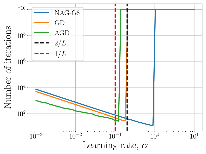
(a) $\mu=1$, $L=10$

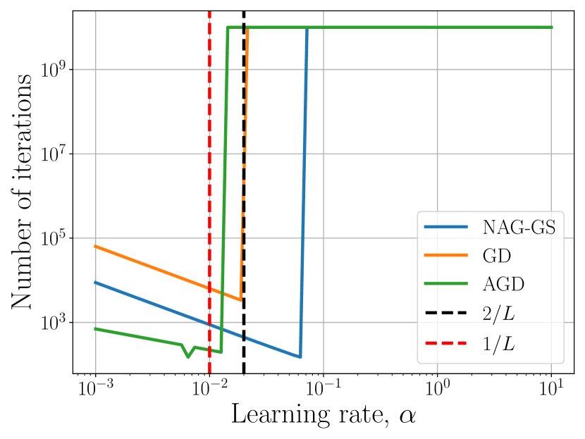
(b) $\mu=10^{-1}$, $L=100$

Figure 1: Dependence of the number of iterations needed for convergence on the learning rate used in the corresponding method. NAG-GS is more robust with respect to the learning rate than gradient descent (GD) and accelerated gradient descent (AGD). Also, NAG-GS converges faster than competitors if the learning rate is sufficiently large. The number of iterations $10^{10}$ indicates the divergence of the method with a corresponding learning rate.

3.2 Logistic regression

In this section, we benchmark NAG-GS method against state-of-the-art optimizers on the logistic regression training problem for MNIST dataset LeCun et al. (2010). Since this problem is convex and non-quadratic, we consider this problem as the natural and next test case after the theoretical analysis and numerical tests of the NAG-GS method in Section 2.3 for the quadratic convex problem. In Figure 2 and Table 2 we present the comparison of the NAG-GS method with competitors. We confirm numerically that the NAG-GS method allows the use of a larger range of values for the learning rate than SGD Momentum and AdamW optimizers. This observation highlights the robustness of our method w.r.t. the selection of hyperparameters. Moreover, the results indicate that the semi-implicit nature of the NAG-GS method indeed ensures the acceleration effect through the use of larger learning rates while keeping a high accuracy of the model, and this holds not only for the convex quadratic problems but also for non-quadratic convex ones.

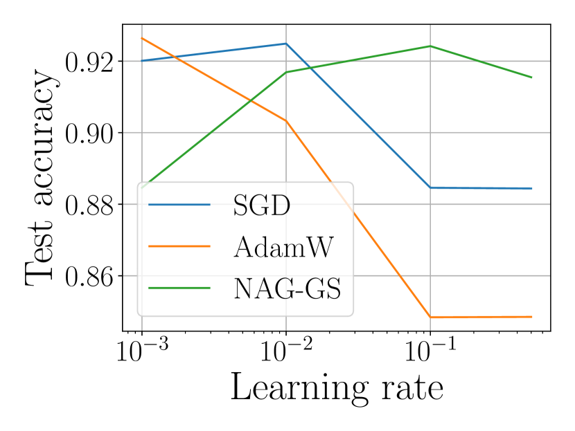
(a) $\mu=1$

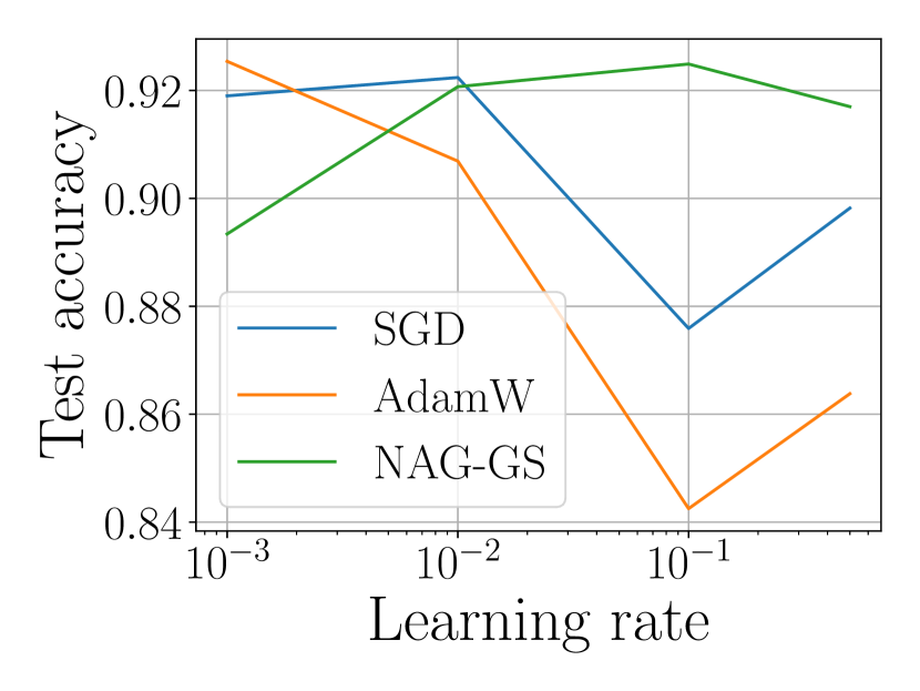
(b) $\mu=10^{-5}$

Figure 2: Dependence of the test accuracy on the learning rates for the considered methods. NAG-GS provides the highest test accuracy for the larger learning rate. This trend preserves for considered $\mu$ of different orders.

Table 2: Test accuracies for NAG-GS, SGD-Momentum, and AdamW for the logistic regression model and MNIST classification problem. NAG-GS gives higher test accuracy for large learning rates, which indicates that it is more robust and does not diverge while learning rate is increased.

Learning rate	NAG-GS	SGD	AdamW
$10^{-3}$	$0.8934$	$0.9190$	$\mathbf{0.9254}$
$10^{-2}$	$0.9207$	$\mathbf{0.9224}$	$0.9069$
$0.1$	$\mathbf{0.9249}$	$0.8759$	$0.8425$
$0.5$	$\mathbf{0.9170}$	$0.8982$	$0.8638$

3.3 Transformer Models

3.3.1 RoBERTa

In this section we test NAG-GS optimizer in the frame of natural language processing for the tasks of fine-tuning pretrained model on GLUE benchmark datasets Wang et al. (2018). We use pretrained RoBERTa Liu et al. (2019) model from Hugging Face’s transformers Wolf et al. (2020) library. In this benchmark, the reference optimizer is AdamW Ilya et al. (2019) with polynomial learning rate schedule. The training setup defined in Liu et al. (2019) is used for both NAG-GS and AdamW optimizers. We search for an optimal learning rate for NAG-GS optimizer with fixed $\gamma$ and $\mu$ to get the best performance on the task at hand. Note that NAG-GS is used with constant schedule which makes it simpler to tune. In terms of learning rate values, the one allowed by AdamW is around $10^{-5}$ while NAG-GS allows a much bigger value of $10^{-2}$. Evaluation results on GLUE tasks are presented in Table 3. Despite a rather restrained search space for NAG-GS hyperparameters, it demonstrates better performance on some tasks and competitive performance on others. Figure 3 shows the behavior of loss values and target metrics on GLUE.

Table 3: Comparison of AdamW and NAG-GS optimizers in fine-tuning on GLUE benchmark. We use reported hyperparameters for AdamW. In the case of NAG-GS, we search hyperparameters space for the best performance metric. Search space consists of learning rate $\alpha$ from $[10^{-3},\,10^{0}]$, factor $\gamma$ from $[10^{-2},\,10^{0}]$, and momentum $\mu=1$.

Optimizer	CoLA	MNLI	MRPC	QNLI	QQP	RTE	SST2	STS-B	WNLI
AdamW	61.60	87.56	88.24	92.62	91.69	78.34	94.95	90.68	56.34
NAG-GS	61.60	87.24	90.69	92.59	91.01	77.97	94.50	90.21	56.34

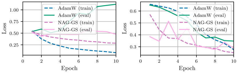
Figure 3: Cross-entropy losses on validation and train sets for CoLA (left) and MRPC (right) tasks. Solid lines correspond to the best trial with the NAG-GS optimizer.

3.3.2 Vision Transformer model

We used the Vision Transformer model Wu et al. (2020), which was pretrained on the ImageNet dataset Deng et al. (2009), and fine-tuned it on the food101 dataset Bossard et al. (2014) using NAG-GS and AdamW. It is worth noting that all weights were updated during the fine-tuning. This task involves classifying a dataset of 101 food categories, with 1000 images per class. To ensure a fair comparison, we first conducted an intensive hyperparameter search Biewald (2020) for all possible hyperparameter configurations on a subset of the data for each of the methods and selected the best configuration. After the hyperparameter search, we performed the experiments on the entire dataset. The results are presented in Table 4. We observed that properly-tuned NAG-GS outperformed AdamW in both training and evaluation metrics. Also, NAG-GS reached higher accuracy compared to AdamW after one epoch. The optimal hyperparameters found for NAG-GS are $\alpha=0.07929,\gamma=0.3554,\mu=0.1301$; for AdamW $\mathrm{lr}=0.00004949,\beta_{1}=0.8679,\beta_{2}=0.9969$.

Table 4: Test accuracies for NAG-GS and AdamW.

Stage	NAG-GS	AdamW
After 1 epoch	$\mathbf{0.8419}$	$0.8269$
After 25 epochs	$\mathbf{0.8606}$	$0.8324$

3.4 ResNet-20 and VGG-11

We compare NAG-GS and momentum SGD with weight decay (SGD-MW) on ResNet-20 He et al. (2016) and VGG-11 Simonyan & Zisserman (2014) models. In particular, we choose these architectures for versatile experimental verification of properties of our optimizer.

ResNet-20.

We carried out intensive experiments in order to deeply evaluate the performance of NAG-GS for computer vision tasks (residual networks in particular) and to show that NAG-GS with the appropriate choice of optimizer parameters is on par with SGD-MW (see Table 1 and Figure 4). For the latter, we use the parameters reported in the literature. The classification problem is solved using CIFAR-10 Krizhevsky (2009). The experimental setup is the same in all experiments except optimizer and its parameters. The best test score for NAG-GS is achieved for $\alpha=0.11$, $\gamma=17$, and $\mu=0.01$.

Figure 4: Evaluation of NAG-GS with SGD-MW on ResNet-20 on CIFAR-10.

VGG-11.

We test this architecture on the CIFAR-10 image classification problem without data resizing and demonstrate the robustness of the NAG-GS optimizer to large learning rates compared to SGD-MW. The hyperparameters are the following: batch size equals to 1000, number of epoch is 50. We use the constant $\gamma=1.$ and $\mu=10^{-4}$ equal to the weight decay parameter in SGD-MW. Also, momentum term in SGD-MW equals to $0.9$. Comparison results are presented in Table 5, where the resulting test accuracy after 50 epochs are given. From this table follows that NAG-GS preserves the expected behaviour to show higher test accuracy in the large learning rate regime compared to SGD-MW optimizer.

Table 5: Test accuracies for NAG-GS and SGD-MW (SGD with momentum and weight decay) for CIFAR-10 classification task on VGG-11 model. NAG-GS gives higher test accuracy for large learning rates to confirm that it is more robust and does not diverge while learning rate is increased.

Learning rate	NAG-GS	SGD-MW
$10^{-3}$	$0.1$	$\mathbf{0.65}$
$10^{-2}$	$0.62$	$\mathbf{0.74}$
$0.1$	$\mathbf{0.76}$	$0.1$
$0.2$	$\mathbf{0.76}$	$0.1$

4 Related works

The approach of interpreting and analyzing optimization methods from the ODEs discretization perspective is well-known and widely used in practice Muehlebach & Jordan (2019); Wilson et al. (2021); Shi et al. (2021). The main advantage of this approach is to construct a direct correspondence between the properties of some classes of ODEs and their associated optimization methods. In particular, gradient descent and Nesterov accelerated methods are discussed in Su et al. (2014) as a particular discretization of ODEs. In the same perspective, many other optimization methods were analyzed, we can mention the mirror descent method and its accelerated versions Krichene et al. (2015), the proximal methods Attouch et al. (2019) and ADMM Franca et al. (2018). It is well known that discretization strategy is essential for transforming a particular ODE to an efficient optimization method, Shi et al. (2019); Zhang et al. (2018) investigate the most proper discretization techniques for different classes of ODEs. A similar analysis but for stochastic first-order methods is presented in Laborde & Oberman (2020); Malladi et al. (2022).

5 Conclusions and further works

We have presented a new and theoretically motivated stochastic optimizer called NAG-GS. It comes from the semi-implicit Gauss-Seidel type discretization of a well-chosen accelerated Nesterov-like SDE. These building blocks ensure two central properties for NAG-GS: (1) the ability to accelerate the optimization process and (2) better robustness to large learning rates. We demonstrate these features theoretically and provide a detailed analysis of the convergence of the method in the quadratic case. Moreover, we show that NAG-GS is competitive with state-of-the-art methods for tackling a wide variety of stochastic optimization problems of increasing complexity and dimension, starting from the logistic regression model to the training of large machine learning models such as ResNet-20, VGG-11 and Transformers. In all tests, NAG-GS demonstrates competitive performance compared with standard optimizers. Further works will focus on the non-asymptotic convergence analysis of NAG-GS for general convex functions and the derivation of efficient and tractable higher-order methods based on the full-implicit discretization of the accelerated Nesterov-like SDE.

Appendix A Additional remarks related to theoretical background

An accelerated ODE has been presented in the main text Section 1.1 which relied on a specific spectral transformation. In this brief section, we add some useful insights:

• Equation (10) is a variant of the heavy ball model with variable damping coefficients in front of $\ddot{x}$ and $\dot{x}$.

• Thanks to the scaling factor $\gamma$ , both the convex case $\mu=0$ and the strongly convex case $\mu>0$ can be handled in a unified way.

• In the continuous time, one can solve easily (8) as follows: $\gamma(t)=\mu+(\gamma_{0}-\mu)e^{-t},\quad t\geq 0$. Since $\gamma_{0}>0$, we have that $\gamma(t)>0$ for all $t\geq 0$ and $\gamma(t)$ converges to $\mu$ exponentially and monotonically as $t\rightarrow+\infty$. In particular, if $\gamma_{0}=\mu>0$, then $\gamma(t)=\mu$ for all $t\geq 0$. We remark here the links between the behavior of the scaling factor $\gamma(t)$ and the sequence $\{\gamma_{k}\}_{k=0}^{\infty}$ introduced by Nesterov Nesterov (2018) in its analysis of optimal first-order methods in discrete-time, see (Nesterov, 2018, Lemma 2.2.3).

• Authors from Luo & Chen (2021) prove the exponential decay property $\mathcal{L}(t)\leq e^{-t}\mathcal{L}_{0},\quad t>0$ for a Taylored Lyapunov function $\mathcal{L}(t):=f(x(t))-f(x^{\star})+\frac{\gamma(t)}{2}\|v(t)-x^{\star}\|^{2}$ where $x^{\star}\in$ argmin $f$ is a global minimizer of $f$. Again we note the similarity between the Lyapunov function proposed here and the estimating sequence $\{\phi_{k}(x)\}_{k=0}^{\infty}$ of function $f$ introduced by Nesterov in its optimal first-order methods analysis Nesterov (2018). In (Nesterov, 2018, Lemma 2.2.3), this sequence that takes the form $\phi_{k}(x)=\phi_{k}^{\star}(x)+\frac{\gamma_{k}}{2}\|v_{k}-x\|^{2}$ where $\gamma_{k+1}:=(1-\alpha_{k})\gamma_{k}+\alpha_{k}\mu$ and $v_{k+1}:=\frac{1}{\gamma_{k+1}}[(1-\alpha_{k})\gamma_{k}v_{k}+\alpha_{k}\mu y_{k}-\alpha_{k}\nabla f(y_{k})]$ which stand for a forward Euler discretization respectively of (8) and second ODE of (9).

We ask the attentive reader to remember that this discussion mainly concerns the continuous time case. A second central part of our analysis was based on the methods of discretization of (9). Indeed, these discretizations ensure together with the spectral transformation (7) the optimal convergence rates of the methods and their particular ability to handle noisy gradients.

A.1 Convergence/Stability analysis of the quadratic case: details

As briefly mentioned in Section 2.3 of the main text, the two key elements to come up with a maximum (constant) step size for Algorithm 1 are the study of the spectral radius of iteration matrix associated with NAG-GS scheme (Section A.1.1) and the covariance matrix at stationarity (Section A.1.2) w.r.t. all the significant parameters of the scheme. These parameters are the step size (integration step/time step) $\alpha$, the convexity parameters $0\leq\mu\leq L\leq\infty$ of the function $f(x)$, the variance of the noise $\sigma^{2}$ and the positive scaling parameter $\gamma$. Note that this theoretical study only concerns the case $f(x)=\frac{1}{2}x^{\top}Ax$.

Reproducibility

• In Section A.1.1, we start by determining the explicit formulation of the spectral radius of the iteration matrix $\rho(E(\alpha))$, specifically for the 2-dimensional quadratic case. This formulation allows us to derive the optimal step size $\alpha_{c}$ that minimizes $\rho(E(\alpha))$, resulting in the highest convergence rate for NAG-GS method. Notably, Lemma 2 presents a crucial outcome for the asymptotic convergence analysis of NAG-GS, revealing that $\rho(E(\alpha))$ is a strictly monotonically increasing function of $\alpha$ within a certain interval, under mild assumptions.

• In Section A.1.2, we conduct an in-depth analysis of the covariance matrix at stationarity, which enables us to establish the sufficient conditions for $\alpha_{c}$ to ensure the asymptotic convergence of the NAG-GS method. The formal proof for this convergence is presented in Lemma 3 for the case of $n=2$.

• In Section A.1.4, we provide the formal proof of Theorem 1, which is enunciated in the main text. This theorem stated the asymptotic convergence of the NAG-GS method for dimensions $n>2$.

A.1.1 Spectral radius analysis

Let us assume $f(x)=\frac{1}{2}x^{\top}Ax$ and since $A\in\mathbb{S}^{n}_{+}$ by hypothesis, it is diagonalizable and can be presented as $A=\text{diag}(\lambda_{1},\ldots,\lambda_{n})$ without loss of generality, that is to say, that we will consider a system of coordinates composed of the eigenvectors of matrix $A$. Let us note that $\mu=\lambda_{1}\leq\ldots\leq\lambda_{n}=L$.

For the following we restrict the discussion to the case $n=2$. In this setting, $y=(x,v)\in\mathbb{R}^{4}$ and the matrices $M$ and $N$ from the Gauss-Seidel splitting of $G_{NAG}$ (7) are:

$$M =\begin{bmatrix}-I_{2\times 2}&0_{2\times 2}\\ \mu/\gamma I_{2\times 2}-A/\gamma&-\mu/\gamma I_{2\times 2}\end{bmatrix}=\begin{bmatrix}-1&0&0&0\\ 0&-1&0&0\\ 0&0&-\mu/\gamma&0\\ 0&\mu/\gamma-L/\gamma&0&-\mu/\gamma\\ \end{bmatrix},$$

$$N =\begin{bmatrix}0_{2\times 2}&I_{2\times 2}\\ 0_{2\times 2}&0_{2\times 2}\end{bmatrix}$$

For the minimization of $f(x)=\frac{1}{2}x^{\top}Ax$, given the property of Brownian motion $\Delta W_{k}=W_{k+1}-W_{k}=\sqrt{\alpha_{k}}\eta_{k}$ where $\eta_{k}\sim\mathcal{N}(0,1)$, (12) reads:

$$y_{k+1} =(I_{4\times 4}-\alpha M)^{-1}(I_{4\times 4}+\alpha N)y_{k}+(I_{4\times 4}-\alpha M)^{-1}\begin{bmatrix}0\\ \sigma\sqrt{\alpha}\eta_{k}\end{bmatrix}$$ (16)

Since matrix $M$ is lower-triangular, matrix $I_{4\times 4}-\alpha M$ is as well and can be factorized as follows:

$$I_{4\times 4}-\alpha M =DT$$

$$=\begin{bmatrix}(1+\alpha)I_{2\times 2}&0_{2\times 2}\\ 0_{2\times 2}&(1+\frac{\alpha\mu}{\gamma})I_{2\times 2}\end{bmatrix}\begin{bmatrix}I_{2\times 2}&0_{2\times 2}\\ \frac{\alpha(A-\mu I_{2\times 2})}{\gamma(1+\frac{\alpha\mu}{\gamma})}&I_{2\times 2}\end{bmatrix}$$

Hence $(I_{4\times 4}-\alpha M)^{-1}=T^{-1}D^{-1}$ where $D^{-1}$ can be easily computed. It remains to compute $T^{-1}$; $T$ can be decomposed as follows: $T=I_{4\times 4}+Q$ with $Q$ a nilpotent matrix such that $QQ=O_{4\times 4}$. For such decomposition, it is well known that:

$$T^{-1}=(I_{4\times 4}+Q)^{-1}=I_{4\times 4}-Q=\begin{bmatrix}I_{2\times 2}&0_{2\times 2}\\ \frac{\alpha(\mu I_{2\times 2}-A)}{\gamma(1+\tau_{k})}&I_{2\times 2}\end{bmatrix}$$ (17)

where $\tau_{k}=\frac{\alpha\mu}{\gamma}$. Combining these results, equation 16 finally reads:

$$y_{k+1} =\begin{bmatrix}\frac{1}{\alpha+1}&0&\frac{\alpha}{1+\alpha}&0\\ 0&\frac{1}{\alpha+1}&0&\frac{\alpha}{1+\alpha}\\ 0&0&\frac{1}{1+\tau}&0\\ 0&\frac{\alpha(\mu-L)}{\gamma(\tau+1)(\alpha+1)}&0&\frac{\alpha^{2}(\mu-L)}{\gamma(1+\tau)(1+\alpha)}+\frac{1}{1+\tau}\end{bmatrix}y_{k}+\begin{bmatrix}0\\ \sigma\frac{\sqrt{\alpha}}{1+\tau}\eta_{k}\end{bmatrix}$$ (18)

$$=Ey_{k}+\begin{bmatrix}0\\ \sigma\frac{\sqrt{\alpha}}{1+\tau}\eta_{k}\end{bmatrix}$$

with $E$ denoting the iteration matrix associated with the NAG-GS method. Hence equation 18 includes two terms, the first is the product of the iteration matrix times the current vector $y_{k}$ and the second one features the effect of the noise. For the latter, it will be studied in Section A.1.2 from the point of view of maximum step size for the NAG-GS method through the key quantity of the covariance matrix. Let us focus on the first term. It is clear that in order to get the maximum contraction rate, we should look for $\alpha$ that minimizes the spectral radius of $E$. Since the spectral radius is the maximum absolute value of the eigenvalues of iteration matrix $E$, we start by computing them. Let us find the expression of $\lambda_{i}\in\sigma(E)$ for $1\leq i\leq 4$ that satisfies $\det(E-\lambda I_{4\times 4})=0$ as functions of the scheme’s parameters. Solving

leads to the following eigenvalues:

$$\lambda_{1} =\frac{\gamma}{\gamma+\alpha\mu}$$ (20)

$$\lambda_{2} =\frac{1}{1+\alpha}$$

$$\lambda_{3} =\frac{2\gamma+\alpha\gamma+\alpha\mu-L\alpha^{2}+\alpha^{2}\mu}{2(\gamma+\alpha\gamma+\alpha\mu+\alpha^{2}\mu)}+$$

$$\frac{\alpha\sqrt{L^{2}\alpha^{2}-2L\alpha^{2}\mu-2L\alpha\mu-2\gamma L\alpha-4\gamma L+\alpha^{2}\mu^{2}+2\alpha\mu^{2}+2\gamma\alpha\mu+\mu^{2}+2\gamma\mu+\gamma^{2}}}{2(\gamma+\alpha\gamma+\alpha\mu+\alpha^{2}\mu)}$$

$$\lambda_{4} =\frac{2\gamma+\alpha\gamma+\alpha\mu-L\alpha^{2}+\alpha^{2}\mu}{2(\gamma+\alpha\gamma+\alpha\mu+\alpha^{2}\mu)}-$$

$$\frac{\alpha\sqrt{L^{2}\alpha^{2}-2L\alpha^{2}\mu-2L\alpha\mu-2\gamma L\alpha-4\gamma L+\alpha^{2}\mu^{2}+2\alpha\mu^{2}+2\gamma\alpha\mu+\mu^{2}+2\gamma\mu+\gamma^{2}}}{2(\gamma+\alpha\gamma+\alpha\mu+\alpha^{2}\mu)}$$

Let us first mention some general behavior or these eigenvalues. Given $\gamma$ and $\mu$ positive, we observe that:

1. $\lambda_{1}$ and $\lambda_{2}$ are positive decreasing functions w.r.t. $\alpha$. Moreover, for bounded $\gamma$ and $\mu$, we have $\lim_{\alpha\to\infty}|\lambda_{1}(\alpha)|=0=\lim_{\alpha\to\infty}|\lambda_{2}(\alpha)|$.

2. One can show that for $\alpha\in[\frac{\mu+\gamma-2\sqrt{\gamma L}}{L-\mu},\frac{\mu+\gamma+2\sqrt{\gamma L}}{L-\mu}]$, functions $\lambda_{3}(\alpha)$ and $\lambda_{4}(\alpha)$ are complex values and one can easily show that both share the same absolute value. Note that the lower bound of the interval $\frac{\mu+\gamma-2\sqrt{\gamma L}}{L-\mu}$ is negative as soon as $\gamma\in[2L-\mu-2\sqrt{L^{2}-\mu L},2L-\mu+2\sqrt{L^{2}-\mu L}]\subseteq\mathbb{R}_{+}$. Moreover, one can easily show that $\lim_{\alpha\to\infty}|\lambda_{3}(\alpha)|=0$ and $\lim_{\alpha\to\infty}|\lambda_{4}(\alpha)|=\frac{L-\mu}{\mu}=\kappa(A)-1$. The latter limit shows that eigenvalue $\lambda_{4}$ plays a central role in the convergence of the NAG-GS method since it is the one that can reach the value one and violate the convergence condition, as soon as $\kappa(A)>2$. The analysis of $\lambda_{4}$ also allows us to come up with a good candidate for the step size $\alpha$ that minimizes the spectral radius of matrix $E$, especially and obviously at critical point $\alpha_{max}=\frac{\mu+\gamma+2\sqrt{\gamma L}}{L-\mu}$ which is positive since $L\geq\mu$ by hypothesis. Note that the case $L\to\mu$ gives some preliminary hints that the maximum step size can be almost "unbounded" in some particular cases.

Now, let us study these eigenvalues in more detail, it seems that three different scenarios must be studied:

1. For any variant of Algorithm 1 for which $\gamma_{0}=\mu$, then $\gamma=\mu$ for all $k\geq 0$ and therefore $\lambda_{1}(\alpha)=\lambda_{2}(\alpha)$. Moreover, at $\alpha=\frac{\mu+\gamma+2\sqrt{\gamma L}}{L-\mu}=\frac{2\mu+2\sqrt{\mu L}}{L-\mu}$, we can easily check that $|\lambda_{1}(\alpha)|=|\lambda_{2}(\alpha)|=|\lambda_{3}(\alpha)|=|\lambda_{4}(\alpha)|$. Therefore $\alpha=\frac{2\mu+2\sqrt{\mu L}}{L-\mu}$ is the step size ensuring the minimal spectral radius and hence the maximum contraction rate. Figure 5 shows the evolution of the absolute values of the eigenvalues of iteration matrix $E$ w.r.t. $\alpha$ for such a setting.

2. As soon as $\gamma<\mu$, one can easily show that $\lambda_{1}(\alpha)<\lambda_{2}(\alpha)$. Therefore the step size $\alpha$ with the minimal spectral radius is such that $|\lambda_{4}(\alpha)|=|\lambda_{2}(\alpha)|$. One can show that the equality holds for $\alpha=\frac{\mu+\gamma+\sqrt{(\mu-\gamma)^{2}+4\gamma L}}{L-\mu}$. One can easily check that $\frac{\mu+\gamma+\sqrt{(\mu-\gamma)^{2}+4\gamma L}}{L-\mu}-\frac{\mu+\gamma+2\sqrt{\gamma L}}{L-\mu}=(\mu-\gamma)^{2}>0$. Hence the second candidate for step size $\alpha$ will be bigger than the first one and the distance between them increases as the squared distance between $\gamma$ and $\mu$. Figure 6 shows the evolution of the absolute values of the eigenvalues of iteration matrix $E$ w.r.t. $\alpha$ for this setting.

3. For $\gamma>\mu$: the analysis of this case gives the same results as the previous point. According to Algorithm 1, $\gamma$ is either constant and equal to $\mu$ or decreasing to $\mu$ along iterations. Hence, the case $\gamma>\mu$ will be considered for the theoretical analysis when $\gamma\neq\mu$.

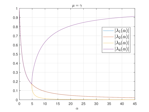
Figure 5: Evolution of absolute values of $\lambda_{i}$ w.r.t $\alpha$; $\mu=\gamma$.

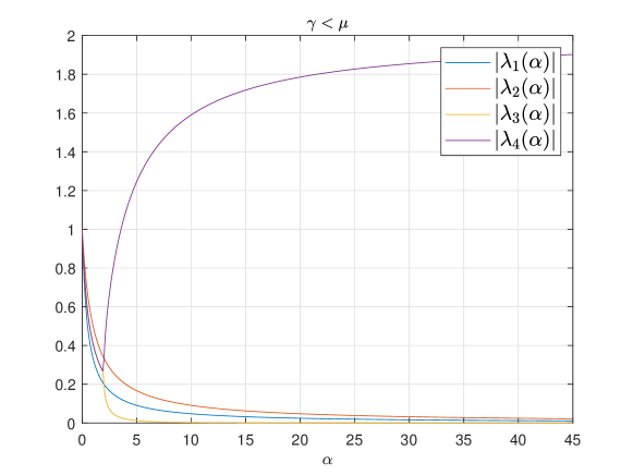
Figure 6: Evolution of absolute values of $\lambda_{i}$ w.r.t $\alpha$; $\gamma<\mu$.

As a first summary, the detailed analysis of the eigenvalues of iteration matrix $E$ w.r.t. the significant parameters of the NAG-GS method leads us to come up with two candidates for the step size that minimize the spectral radius of $E$, hence ensuring the highest contraction rate possible. These results will be gathered with those obtained in Section A.1.2 dedicated to the covariance matrix analysis.

Let us now look at the behavior of the dynamics in expectation; given the properties of the Brownian motion and by applying the Expectation operator $\mathbb{E}$ on both sides of the system of SDE’s (11), the resulting "averaged" equations identify with the "deterministic" setting studied by Luo & Chen (2021). For such a setting, authors from Luo & Chen (2021) demonstrated that, if $0\leq\alpha\leq\frac{2}{\sqrt{\kappa(A)}}$, then a Gauss–Seidel splitting-based scheme for solving (9) is A-stable for quadratic objectives in the deterministic setting. We conclude this section by showing that the two candidates we derived above for step size are higher than the limit $\frac{2}{\sqrt{\kappa(A)}}$ given in (Luo & Chen, 2021, Theorem 1). It can be intuitively understood in the case $L\to\mu$, however, we give a formal proof in Lemma 1.

Lemma 1.

Given $\gamma>0$, and assuming $0<\mu<L$, then for $\gamma=\mu$ and $\gamma>\mu$ the following inequalities respectively hold:

$$\frac{2\mu+2\sqrt{\mu L}}{L-\mu} >\frac{2}{\sqrt{\kappa(A)}}$$ (21)

$$\frac{\mu+\gamma+\sqrt{(\mu-\gamma)^{2}+4\gamma L}}{L-\mu} >\frac{2}{\sqrt{\kappa(A)}}$$

where $\kappa(A)=\frac{L}{\mu}$.

Proof.

Let us start for the case $\mu=\gamma$, hence first inequality from equation 21 becomes:

$$\frac{2\mu+2\sqrt{L\mu}}{L-\mu}>\frac{2}{\sqrt{L/\mu}}$$

$$\equiv (\mu+\sqrt{L\mu})\sqrt{L/\mu}>(L-\mu)$$

$$\equiv \sqrt{\mu L}+L>L-\mu$$

$$\equiv \sqrt{\mu L}>-\mu$$

which holds for any positive $\mu,L$ and satisfied by hypothesis. For the case $\gamma>\mu$, we have:

$$\frac{\mu+\gamma+\sqrt{(\mu-\gamma)^{2}+4\gamma L}}{L-\mu}>\frac{2}{\sqrt{L/\mu}}$$

$$\equiv \sqrt{(\mu-\gamma)^{2}+4\gamma L}>\frac{2}{\sqrt{L/\mu}}(L-\mu)-\gamma-\mu$$

$$\equiv (\mu-\gamma)^{2}+4\gamma L>(\mu+2\sqrt{\frac{\mu}{L}}(\mu-L)+\gamma)^{2}$$

$$\equiv \gamma>\frac{-2\mu^{2}+\mu^{3}/L+\mu^{2}\sqrt{\mu/L}+\mu L-\mu L\sqrt{\mu/L}}{-\mu-\sqrt{\mu/L}(\mu-L)+L}$$

where second inequality hold since $L\geq\mu$ and last inequality holds since $-\mu-\sqrt{\mu/L}(\mu-L)+L>0$ (one can easily check this by using $L>\mu$). It remains to show that:

$$\mu>\frac{-2\mu^{2}+\mu^{3}/L+\mu^{2}\sqrt{\mu/L}+\mu L-\mu L\sqrt{\mu/L}}{-\mu-\sqrt{\mu/L}(\mu-L)+L}$$

which holds for any $\mu$ and $L$ positive (technical details are skipped; it mainly consists of the study of a table of signs of a polynomial equation in $\mu$).

Since $\gamma>\mu$ by hypothesis, therefore inequality

$$\gamma>\frac{-2\mu^{2}+\mu^{3}/L+\mu^{2}\sqrt{\mu/L}+\mu L-\mu L\sqrt{\mu/L}}{-\mu-\sqrt{\mu/L}(\mu-L)+L}$$

holds for any $\mu$ and $L$ positive as well, conditions satisfied by hypothesis. This concludes the proof.

∎

Furthermore, let us note that both step size candidates, that are $\{\frac{2\mu+2\sqrt{\mu L}}{L-\mu},\frac{\mu+\gamma+\sqrt{(\mu-\gamma)^{2}+4\gamma L}}{L-\mu}\}$ respectively for the cases $\gamma=\mu$ and $\gamma>\mu$ show that NAG-GS method converges in the case $L\to\mu$ with a step size that tends to $\infty$, this behavior cannot be anticipated by the upper-bound given by (Luo & Chen, 2021, Theorem 1). Some simple numerical experiments are performed in Section A.1.5 to support this theoretical result.

Finally, based on previous discussions, let us remark that for $\alpha\in[\frac{\mu+\gamma+\sqrt{(\mu-\gamma)^{2}+4\gamma L}}{L-\mu},\infty]$ when $\gamma\neq\mu$ or $\alpha\in[\frac{2\mu+2\sqrt{\mu L}}{L-\mu},\infty]$ when $\gamma=\mu$, we have $\rho(E(\alpha))=|\lambda_{4}(\alpha)|$ and one can show that $\rho(E)$ is strictly monotonically increasing function of $\alpha$ for all $L>\mu>0$ and $\gamma>0$, see Lemma 2 for the formal proof.

Lemma 2.

Given $\gamma>0$, and assuming $0<\mu<L$, then for $\gamma=\mu$ and $\gamma>\mu$, the spectral radius $\rho(E(\alpha))$ is a strict monotonic increasing function of $\alpha$ for $\alpha\in[\alpha_{c},\infty]$ with $\alpha_{c}=\frac{2\mu+2\sqrt{\mu L}}{L-\mu}$ or $\alpha_{c}=\frac{\mu+\gamma+\sqrt{(\mu-\gamma)^{2}+4\gamma L}}{L-\mu}$.

Proof.

Let us first recall that on $[\alpha_{c},\infty]$, the spectral radius $\rho(E(\alpha))$ is equal to $|\lambda_{4}|$, the expression of $\lambda_{4}$ as a function of parameters of interests for the convergence analysis of NAG-GS method was given in equation 20 and recalled here-under for convenience:

$$\lambda_{4} =\frac{2\gamma+\alpha\gamma+\alpha\mu-L\alpha^{2}+\alpha^{2}\mu}{2(\gamma+\alpha\gamma+\alpha\mu+\alpha^{2}\mu)}-$$ (22)

$$\frac{\alpha\sqrt{L^{2}\alpha^{2}-2L\alpha^{2}\mu-2L\alpha\mu-2\gamma L\alpha-4\gamma L+\alpha^{2}\mu^{2}+2\alpha\mu^{2}+2\gamma\alpha\mu+\mu^{2}+2\gamma\mu+\gamma^{2}}}{2(\gamma+\alpha\gamma+\alpha\mu+\alpha^{2}\mu)}$$

Let start by showing that $\lambda_{4}$ is negative on $[\alpha_{c},\infty]$. Firstly, one can easily observe that the denominator of $\lambda_{4}$ is positive, secondly let us compute the values for $\alpha$ such that:

$$2\gamma+\alpha\gamma+\alpha\mu-L\alpha^{2}+\alpha^{2}\mu-$$ (23)

$$\alpha\sqrt{L^{2}\alpha^{2}-2L\alpha^{2}\mu-2L\alpha\mu-2\gamma L\alpha-4\gamma L+\alpha^{2}\mu^{2}+2\alpha\mu^{2}+2\gamma\alpha\mu+\mu^{2}+2\gamma\mu+\gamma^{2}}=0$$

$$\equiv -4\gamma^{2}-4\alpha\gamma(\mu+\gamma)+\alpha^{2}(\gamma^{2}-4\gamma L+2\gamma\mu+\mu^{2})-\alpha^{2}(\gamma^{2}-4\gamma L+6\gamma\mu+\mu^{2})=0$$

$$\equiv (-4\gamma\mu)\alpha^{2}-4\gamma(\mu+\gamma)\alpha-4\gamma^{2}=0$$

The expression above is negative as soon as $\alpha<-1$ or $\alpha>\frac{-\gamma}{\mu}<0$ since $\gamma,\mu>0$ by hypothesis. The latter is always satisfied since $\alpha\geq\alpha_{c}>0$ by hypothesis. Therefore $\rho(E(\alpha))=-\lambda_{4}$ for $\alpha\in[\alpha_{c},\infty]$.

To show the monotonic increasing behavior of $\rho(E(\alpha))$ w.r.t. $\alpha\in[\alpha_{c},\infty]$, it remains to show that:

$$\frac{d(\rho(E(\alpha))}{d\alpha}=\frac{d(-\lambda_{4})}{d\alpha}>0.$$ (24)

To ease the analysis, let us decompose $-\lambda_{4}(\alpha)=t_{1}(\alpha)+t_{2}(\alpha)$ such that:

$$t_{1}(\alpha)=-\frac{2\gamma+\alpha\gamma+\alpha\mu-L\alpha^{2}+\alpha^{2}\mu}{2(\gamma+\alpha\gamma+\alpha\mu+\alpha^{2}\mu)}$$ (25)

$$t_{2}(\alpha)=\frac{\alpha\sqrt{L^{2}\alpha^{2}-2L\alpha^{2}\mu-2L\alpha\mu-2\gamma L\alpha-4\gamma L+\alpha^{2}\mu^{2}+2\alpha\mu^{2}+2\gamma\alpha\mu+\mu^{2}+2\gamma\mu+\gamma^{2}}}{2(\gamma+\alpha\gamma+\alpha\mu+\alpha^{2}\mu)}$$

Let us now show that $\frac{dt_{1}(\alpha)}{d\alpha}>0$ and $\frac{dt_{2}(\alpha)}{d\alpha}>0$ for any $L>\mu>0$. We first obtain:

$$\frac{dt_{1}(\alpha)}{d\alpha} =\frac{(2\gamma+2\mu+4\alpha\mu)(2\gamma+\alpha\gamma+\alpha\mu-L\alpha^{2}+\alpha^{2}\mu)}{(2\gamma+2\alpha\gamma+2\alpha\mu+2\alpha^{2}\mu)^{2}}-$$ (26)

$$\frac{\gamma+\mu-2L\alpha+2\alpha\mu}{2\gamma+2\alpha\gamma+2\alpha\mu+2\alpha^{2}\mu}$$

$$=\frac{(L\alpha^{2}+\gamma)(\gamma+\mu)+2\alpha\gamma(L+\mu)}{2(\alpha+1)^{2}(\gamma+\alpha\mu)^{2}}$$

which is strictly positive since $L>\mu>0$ and $\gamma>0$ by hypothesis. Furthermore:

The remaining demonstration is significantly long and technically heavy in the case $\gamma>\mu$. Then we limit the last part of the demonstration for the case $\mu=\gamma$ for which we have shown previously than $\alpha_{c}=\frac{\mu+\gamma+2\sqrt{\gamma L}}{L-\mu}=\frac{2\mu+2\sqrt{\mu L}}{L-\mu}$. In practice, with respect to the NAG-GS method summarized by Algorithm 1, $\gamma$ quickly decreases to $\mu$ and equality $\mu=\gamma$ holds for the most part of the iterations of the Algorithm, hence this case is more important to detail here. However, the reasoning explained herein ultimately leads to identical final conclusions when considering the case where $\gamma$ is greater than $\mu$.

The first term of the numerator of Equation 27 is positive as soon as $\alpha\geq\sqrt{\frac{3\gamma}{L}}$. In the case $\mu=\gamma$, we determine the conditions under which the second term of the numerator of Equation 27 is positive, that is:

$$\alpha^{2}(L(-2\mu^{2})+2\mu(L^{2}-L\mu+\mu^{2}))+\mu(2\mu^{2}-2\mu(2L-\mu))>0$$ (28)

$$\equiv\alpha^{2}(L(-2\mu^{2})+2\mu(L^{2}-L\mu+\mu^{2}))>\mu(-2\mu^{2}+2\mu(2L-\mu))$$

First one can see that:

$$(L(-2\mu^{2})+2\mu(L^{2}-L\mu+\mu^{2}))>0,$$ (29)

$$\mu(-2\mu^{2}+2\mu(2L-\mu))>0$$

hold as soon as $L>\mu>0$ which is satisfied by hypothesis. Therefore, the second term of the numerator of Equation 27 is positive as soon as

$$\alpha>\sqrt{\frac{\mu(-2\mu^{2}+2\mu(2L-\mu))}{(L(-2\mu^{2})+2\mu(L^{2}-L\mu+\mu^{2}))}}=\sqrt{\frac{2\mu}{L-\mu}}$$ (30)

which exists since $L>\mu>0$ by hypothesis (the second root of equation 29 being negative). Finally, since $\alpha\in[\alpha_{c},\infty]$ by hypothesis, $\frac{dt_{2}(\alpha)}{d\alpha}$ is positive as soon as:

$$\alpha_{c}>\sqrt{\frac{3\mu}{L}}$$ (31)

$$\alpha_{c}>\sqrt{\frac{2\mu}{L-\mu}}$$

hold with $\alpha_{c}=\frac{2\mu+2\sqrt{\mu L}}{L-\mu}$. One can easily show that both inequalities hold as soon as $L>\mu>0$ which is satisfied by the hypothesis. This concludes the proof of the strict increasing monotonicity of $\rho(E(\alpha))$ w.r.t. $\alpha$ for $\alpha\in[\alpha_{c},\infty]$ assuming $L>\mu>0$ and $\gamma=\mu$.

∎

A.1.2 Covariance analysis

In this section, we study the contribution to the computation of maximum step size for the NAG-GS method through the analysis of the covariance matrix at stationarity. Let us start by computing the covariance matrix $C$ obtained at iteration $k+1$ from Algorithm 1:

$$C_{k+1}=\mathbb{E}(y_{k+1}y_{k+1}^{T})$$ (32)

By denoting $\xi_{k}=\begin{bmatrix}0\\ \sigma\frac{\sqrt{\alpha}}{1+\tau}\eta_{k}\end{bmatrix}$, let us replace $y_{k+1}$ by its expression given in equation 18, equation 32 writes:

$$C_{k+1} =\mathbb{E}(y_{k+1}y_{k+1}^{T})$$ (33)

$$=\mathbb{E}\left((Ey_{k}+\xi_{k})(Ey_{k}+\xi_{k})^{T}\right)$$

$$=\mathbb{E}\left(Ey_{k}y_{k}^{T}E^{T}\right)+\mathbb{E}\left(\xi_{k}\xi_{k}^{T}\right)$$

which holds since expectation operator $\mathbb{E}(.)$ is a linear operator and by assuming statistical independence between $\xi_{k}$ and $Ey_{k}$. On the one hand, by using again the properties of linearity of $\mathbb{E}$ and since $E$ is seen as a constant by $\mathbb{E}(.)$, one can show that $\mathbb{E}\left(Ey_{k}y_{k}^{T}E^{T}\right)=EC_{k}E^{T}$. On the other hand, since $\eta_{k}\sim\mathcal{N}(0,1)$, then Equation equation 33 becomes:

$$C_{k+1} =EC_{k}E^{T}+Q$$ (34)

where $Q=\begin{bmatrix}0_{2\times 2}&0_{2\times 2}\\ 0_{2\times 2}&\frac{\alpha_{k}\sigma^{2}}{(1+\tau_{k})^{2}}I_{2\times 2}\end{bmatrix}$. Let us now look at the limiting behavior of Equation equation 34, that is $\lim_{k\to\infty}C_{k}$. Let be $C=\lim_{k\to\infty}C_{k}$ the covariance matrix reached in the asymptotic regime, also referred to as stationary regime. Applying the limit on both sides of Equation equation 34, $C$ then satisfies

$$C =ECE^{T}+Q$$ (35)

Hence equation 35 is a particular case of discrete Lyapunov equation. For solving such equation, the vectorization operator denoted $\vec{.}$ is applied on both sides on equation 35, this amounts to solve the following linear system:

$$(I_{4^{2}\times 4^{2}}-E\otimes E)\vec{C}=\vec{Q}$$ (36)

where $A\otimes B=\begin{bmatrix}a_{11}B&\cdots&a_{1n}B\\ \vdots&\ddots&\vdots\\ a_{m1}B&\cdots&a_{mn}B\end{bmatrix}$ stands for the Kronecker product. The solution is given by:

$$C=\overleftarrow{(I_{4^{2}\times 4^{2}}-E\otimes E)^{-1}\vec{Q}}$$ (37)

where $\overleftarrow{a}$ stands for the un-vectorized operator.

Let us note that, even for the $2$-dimensional case considered in this section, the dimension of matrix $C$ rapidly growth and cannot be written in plain within this paper. For the following, we will keep its symbolic expression. The stationary matrix $C$ quantifies the spreading of the limit of the sequence $\{y_{k}\}$, as a direct consequence of the Brownian motion effect. Now we look at the directions that maximize the scattering of the points, in other words, we are looking for the eigenvectors and the associated eigenvalues of $C$. Actually, the required information for the analysis of the step size is contained within the expression of the eigenvalues $\lambda_{i}(C)$. The obtained eigenvalues are rationale functions w.r.t. the parameters of the schemes, while their numerator brings less interest for us (supported further), we will focus on their denominator. We obtained the following expressions:

$$\lambda_{1}(C) =\frac{N_{1}(\alpha,\mu,L,\gamma,\sigma)}{D_{1}(\alpha,\mu,L,\gamma,\sigma)},$$ (38)

$$\text{s.t. }D_{1}(\alpha,\mu,L,\gamma,\sigma) =-L^{2}\alpha^{3}\mu-L^{2}\alpha^{2}\mu-\gamma L^{2}\alpha^{2}+2L\alpha^{3}\mu^{2}+4L\alpha^{2}\mu^{2}+$$

$$4\gamma L\alpha^{2}\mu+2L\alpha\mu^{2}+8\gamma L\alpha\mu+2\gamma^{2}L\alpha+4\gamma L\mu+4\gamma^{2}L$$

$$\lambda_{2}(C) =\frac{N_{2}(\alpha,\mu,L,\gamma,\sigma)}{D_{2}(\alpha,\mu,L,\gamma,\sigma)},$$ (39)

$$\text{s.t. }D_{2}(\alpha,\mu,L,\gamma,\sigma) =\alpha^{3}\mu^{3}+3\alpha^{2}\mu^{3}+3\gamma\alpha^{2}\mu^{2}+2\alpha\mu^{3}+$$

$$8\gamma\alpha\mu^{2}+2\gamma^{2}\alpha\mu+4\gamma\mu^{2}+4\gamma^{2}\mu$$

$$\lambda_{3}(C) =\frac{N_{3}(\alpha,\mu,L,\gamma,\sigma)}{D_{3}(\alpha,\mu,L,\gamma,\sigma)},$$ (40)

$$\text{s.t. }D_{3}(\alpha,\mu,L,\gamma,\sigma) =\alpha^{3}\mu^{3}+3\alpha^{2}\mu^{3}+3\gamma\alpha^{2}\mu^{2}+2\alpha\mu^{3}+$$

$$8\gamma\alpha\mu^{2}+2\gamma^{2}\alpha\mu+4\gamma\mu^{2}+4\gamma^{2}\mu$$

$$\lambda_{4}(C) =\frac{N_{4}(\alpha,\mu,L,\gamma,\sigma)}{D_{4}(\alpha,\mu,L,\gamma,\sigma)},$$ (41)

$$\text{s.t. }D_{4}(\alpha,\mu,L,\gamma,\sigma) =-L^{2}\alpha^{3}\mu-L^{2}\alpha^{2}\mu-\gamma L^{2}\alpha^{2}+2L\alpha^{3}\mu^{2}+4L\alpha^{2}\mu^{2}+$$

$$4\gamma L\alpha^{2}\mu+2L\alpha\mu^{2}+8\gamma L\alpha\mu+2\gamma^{2}L\alpha+4\gamma L\mu+4\gamma^{2}L$$

One can observe that:

1. Given $\alpha,L,\mu,\gamma$ positive, the denominators of eigenvalues $\lambda_{2}$ and $\lambda_{3}$ are positive as well, unlike eigenvalues $\lambda_{1}$ and $\lambda_{4}$ for which some vertical asymptotes may appear. The latter will be studied in more detail further. Note that, even if some eigenvalues share the same denominator, it is not the case for the numerator. This will be illustrated later in Figures 9 and 10 to ease the analysis.

2. Interestingly, the volatility of the noise defined by the parameter $\sigma$ does not appear within the expressions of the denominators. It gives us a hint that these vertical asymptotes are due to the fact that spectral radius is getting close to 1 (discussed further in Section A.1.3). Moreover, the parameter $\sigma$ appears only within the numerators and based on intensive numerical tests, this parameter has a pure scaling effect onto the eigenvalues $\lambda_{i}(C)$ when studied w.r.t. $\alpha$ without modifying the trends of the curves.

Let us now study in more details the denominator of $\lambda_{1}$ and $\lambda_{4}$ and seek for critical step size as a function of $\gamma,\mu$ and $L$ at which a vertical asymptote may appear by solving:

$$-L^{2}\alpha^{3}\mu-L^{2}\alpha^{2}\mu-\gamma L^{2}\alpha^{2}+2L\alpha^{3}\mu^{2}+4L\alpha^{2}\mu^{2}+$$ (42)

$$4\gamma L\alpha^{2}\mu+2L\alpha\mu^{2}+8\gamma L\alpha\mu+2\gamma^{2}L\alpha+4\gamma L\mu+4\gamma^{2}L=0$$

$$\equiv \mu(2\mu-L)\alpha^{3}+(\mu+\gamma)(4\mu-L)\alpha^{2}+(2\mu^{2}+8\gamma\mu+2\gamma^{2})\alpha+4\gamma(\mu+\gamma)=0$$

This polynomial equation in $\alpha$ has three roots:

$$\alpha_{1} =\frac{-\gamma-\mu}{\mu},$$ (43)

$$\alpha_{2} =\frac{\mu+\gamma-\sqrt{\gamma^{2}-6\gamma\mu+\mu^{2}+4\gamma L}}{L-2\mu},$$

$$\alpha_{3} =\frac{\mu+\gamma+\sqrt{\gamma^{2}-6\gamma\mu+\mu^{2}+4\gamma L}}{L-2\mu}.$$

First, it is obvious that the first root $\alpha_{1}$ is negative given $\gamma,\mu$ assumed nonnegative and therefore can be disregarded. Concerning $\alpha_{2}$ and $\alpha_{3}$, those are real roots as soon as:

$$\gamma^{2}-6\gamma\mu+\mu^{2}+4\gamma L\geq 0$$ (44)

$$\equiv (\gamma-\mu)^{2}-4\gamma\mu+4\gamma L\geq 0$$

$$\equiv (\gamma-\mu)^{2}\geq 4\gamma(\mu-L)$$

which is always satisfied since $\gamma>0$ and $0<\mu<L$ by hypothesis.

Further, it is obvious that the study must include three scenarios:

1. Scenario 1: $L-2\mu<0$, or equivalently $\mu>L/2$. Given $\mu$ and $\gamma$ positive by hypothesis, it implies that $\alpha_{3}$ is negative and hence can be disregarded. It remains to check if $\alpha_{2}$ can be positive, it amounts to verifying if

   $$\mu+\gamma-\sqrt{\gamma^{2}-6\gamma\mu+\mu^{2}+4\gamma L}<0$$

   $$\equiv (\mu+\gamma)^{2}<\gamma^{2}-6\gamma\mu+\mu^{2}+4\gamma L$$

   $$\equiv \mu<\frac{L}{2}$$

   which never holds by hypothesis. Therefore, for the first scenario, there is no positive critical step size at which a vertical asymptote for the eigenvalues may appear.

2. Scenario 2: $L-2\mu>0$, or equivalently $\mu<L/2$. Obviously, $\alpha_{3}$ is positive and hence shall be considered for the analysis of maximum step size for our NAG-GS method. It remains to check if $\alpha_{2}$ is positive, that is to verify if the numerator can be negative. We have seen in the first scenario that $\alpha_{2}$ is negative as soon as $\mu<\frac{L}{2}$ which is verified by hypothesis. Therefore, only $\alpha_{3}$ is positive.

3. Scenario 3: $L-2\mu=0$. For such a situation, the critical step size is located at $\infty$ and can be disregarded as a potential limitation in our study.

In summary, a potentially critical and limiting step size only exists in the case $\mu<L/2$, or equivalently if $\kappa(A)>2$. In this setting, the critical step size is positive and is equal to $\alpha_{\text{crit}}=\frac{\mu+\gamma+\sqrt{\gamma^{2}-6\gamma\mu+\mu^{2}+4\gamma L}}{L-2\mu}$. Figures 7 to 8 display the evolution of the eigenvalues $\lambda_{i}(C)$ for $1\leq i\leq 4$ w.r.t. to $\alpha$ for the two first scenarios, that are for $\mu>L/2$ and $\mu<L/2$. For the first scenario, the parameters $\sigma$, $\gamma$, $\mu$ and $L$ have been respectively set to $\{1,3/2,1,3/2\}$. For the second scenario, $\sigma$, $\gamma$, $\mu$ and $L$ have been respectively set to $\{1,3/2,1,3\}$. As expected, one can observe in Figure 7 that no vertical asymptote is present. Furthermore, one can observe $\lambda_{i}(C)$ seem to converge to some limit point when $\alpha\to\infty$, numerically we report that this limit point is zero, for all the values of $\gamma$ and $\sigma$ considered.

Finally, again as expected by the results presented in this section, Figure 8 shows the presence of two vertical asymptotes for the eigenvalues $\lambda_{1}$ and $\lambda_{4}$, and none for $\lambda_{2}$ and $\lambda_{3}$. Moreover, the critical step size is approximately located at $\alpha=6$ which aligns with analytical expression $\alpha_{\text{crit}}=\frac{\mu+\gamma+\sqrt{\gamma^{2}-6\gamma\mu+\mu^{2}+4\gamma L}}{L-2\mu}$. Finally, one can observe that, after the vertical asymptotes, all the eigenvalues converge to some limit points, again numerically we report that this limit point is zero, for all the values of $\gamma$ and $\sigma$ considered.

Figure 7: Evolution of $\lambda_{i}(C)$ w.r.t $\alpha$ for scenario $\mu>L/2$; $\sigma=1$, $\gamma=3/2$, $\mu=1$, $L=3/2$.

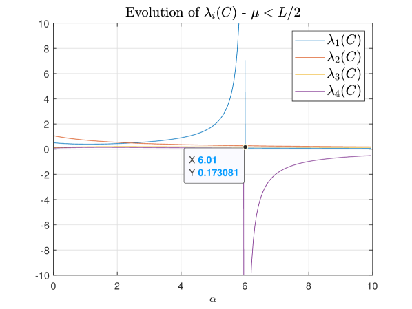
Figure 8: Evolution of $\lambda_{i}(C)$ w.r.t $\alpha$ for scenario $\mu<L/2$; $\sigma=1$, $\gamma=3/2$, $\mu=1$, $L=3$.

A.1.3 A conclusion for the 2-dimensional case

In Section A.1.1 and Section A.1.2, several theoretical results have been derived for coming up with appropriate choices of constant step size for Algorithm 1. Key insights and interesting values for the step size have been discussed from the study of the spectral radius of iteration matrix $E$ and through the analysis of the covariance matrix in the asymptotic regime. Let us summarize the theoretical results obtained:

• from the spectral radius analysis of iteration matrix $E$; two scenarios have been highlighted, that are:

  1. case $\gamma=\mu$: the step size $\alpha$ that minimizes the spectral radius of matrix $E$ is $\alpha=\frac{2\mu+2\sqrt{\mu L}}{L-\mu}$,

  2. case $\gamma>\mu$: the step size $\alpha$ that minimizes the spectral radius of matrix $E$ is $\alpha=\frac{\mu+\gamma+\sqrt{(\mu-\gamma)^{2}+4\gamma L}}{L-\mu}$.

• from the analysis of covariance matrix $C$ at stationarity: in the case $L-2\mu>0$, or equivalently $\mu<L/2$, we have seen that there is a vertical asymptote for two eigenvalues of $C$ at $\alpha_{\text{crit}}=\frac{\mu+\gamma+\sqrt{\gamma^{2}-6\gamma\mu+\mu^{2}+4\gamma L}}{L-2\mu}$, leading to an intractable scattering of the limit points $\{y_{k}\}_{k\to\infty}$ generated by Algorithm 1. In the case $\mu>L/2$, there is no positive critical step size at which a vertical asymptote for the eigenvalues may appear.

Therefore, for quadratic functions such that $\mu>L/2$, we can safely choose either $\alpha=\frac{2\mu+2\sqrt{\mu L}}{L-\mu}$ when $\gamma=\mu$ either $\alpha=\frac{\mu+\gamma+\sqrt{(\mu-\gamma)^{2}+4\gamma L}}{L-\mu}$ when $\gamma>\mu$ to get the minimal spectral radius for iteration matrix $E$ and hence the highest contraction rate for the NAG-GS method.

For quadratic functions such that $\mu<L/2$, we must show that the NAG-GS method is stable for both step sizes. Let us denote by $\alpha_{c}=\{\frac{2\mu+2\sqrt{\mu L}}{L-\mu},\frac{\mu+\gamma+\sqrt{(\mu-\gamma)^{2}+4\gamma L}}{L-\mu}\}$, two values of step size for the two scenarios $\gamma=\mu$ and $\gamma>\mu$. In Lemma 3, we show that NAG-GS is asymptotically convergent, or stable, for the 2-dimensional case under mild assumptions in the case $\mu<L/2$.

Lemma 3.

Given $\gamma>0$, and assuming $0<\mu<L/2$, then for $\gamma=\mu$ and $\gamma>\mu$ the following inequalities respectively hold:

$$\frac{\mu+\gamma+\sqrt{\gamma^{2}-6\gamma\mu+\mu^{2}+4\gamma L}}{L-2\mu} >\frac{2\mu+2\sqrt{\mu L}}{L-\mu}$$ (45)

$$\frac{\mu+\gamma+\sqrt{\gamma^{2}-6\gamma\mu+\mu^{2}+4\gamma L}}{L-2\mu} >\frac{\mu+\gamma+\sqrt{(\mu-\gamma)^{2}+4\gamma L}}{L-\mu}$$

Thus, in the 2-dimensional case, NAG-GS is asymptotically convergent (or stable) when choosing $\alpha_{c}=\frac{\mu+\gamma+\sqrt{(\mu-\gamma)^{2}+4\gamma L}}{L-\mu}$ or $\alpha_{c}=\frac{2\mu+2\sqrt{\mu L}}{L-\mu}$ respectively for the cases $\gamma>\mu$ and $\gamma=\mu$.

Proof.

In order to prove the asymptotic stability or convergence of NAG-GS for the 2-dimensional case within the set of assumptions detailed above, one must show that $\rho(E(\alpha_{c}))<1$ for the two choices of $\alpha_{c}$.

Let us start by computing $\alpha$ such that $\rho(E(\alpha))=1$. As proved in Lemma 2, for $\alpha\in[\alpha_{c},\infty]$, $\rho(E(\alpha))=-\lambda_{4}$ with $\lambda_{4}$ given in equation 20, we then have to compute $\alpha$ such that:

$$-\lambda_{4} =-\frac{2\gamma+\alpha\gamma+\alpha\mu-L\alpha^{2}+\alpha^{2}\mu}{2(\gamma+\alpha\gamma+\alpha\mu+\alpha^{2}\mu)}+$$

$$\frac{\alpha(L^{2}\alpha^{2}-2L\alpha^{2}\mu-2L\alpha\mu-2\gamma L\alpha-4\gamma L+\alpha^{2}\mu^{2}+2\alpha\mu^{2}+2\gamma\alpha\mu+\mu^{2}+2\gamma\mu+\gamma^{2})^{1/2}}{2(\gamma+\alpha\gamma+\alpha\mu+\alpha^{2}\mu)}=1.$$

This leads to computing the roots of a quadratic polynomial equation in $\alpha$, the positive root is:

$$\alpha=\frac{\gamma+\mu+\sqrt{4L\gamma+\gamma^{2}-6\gamma\mu+\mu^{2}}}{L-2\mu}$$ (46)

which not surprisingly identifies to $\alpha_{\text{crit}}$ from the covariance matrix analysis .

Furthermore, as per Lemma 2, $\rho(E(\alpha))$ is strictly monotonically increasing function over the interval $[\alpha_{c},\infty]$. Therefore, showing that $\rho(E(\alpha_{c}))<1$ is equivalent to show that $\alpha_{c}$ is strictly lower than $\alpha_{\text{crit}}:=\frac{\gamma+\mu+\sqrt{4L\gamma+\gamma^{2}-6\gamma\mu+\mu^{2}}}{L-2\mu}$.

Let us focus on the case $\gamma>\mu$; since $0<\mu<L/2$ by hypothesis, the second inequality from equation 45 can be written as:

$$(L-\mu)(\gamma+\mu+\sqrt{(\gamma-\mu)^{2}+4\gamma(L-\mu)})-(L-2\mu)(\gamma+\mu+\sqrt{(\gamma-\mu)^{2}+4\gamma L})>0$$

$$\equiv \gamma\mu+\mu^{2}+(L-\mu)\sqrt{\gamma^{2}+\mu^{2}+\gamma(4L-6\mu)}+(2\mu-L)\sqrt{(\gamma-\mu)^{2}+4\gamma L}>0$$

Given $\gamma,\mu>0$, it remains to show that:

$$(L-\mu)\sqrt{\gamma^{2}+\mu^{2}+\gamma(4L-6\mu)}+(2\mu-L)\sqrt{(\gamma-\mu)^{2}+4\gamma L}>0$$ (47)

In order to show this, we study the conditions for $\gamma$ such that the left-hand side of equation 47 is positive. With simple manipulations, one can show that canceling the left-hand side of equation 47 boils down to canceling the following quadratic polynomial:

$$(L-\mu)\sqrt{\gamma^{2}+\mu^{2}+\gamma(4L-6\mu)}+(2\mu-L)\sqrt{(\gamma-\mu)^{2}+4\gamma L} =0$$

$$\equiv(-3\mu+2L)\gamma^{2}+(2\mu^{2}-8L\mu+4L^{2})\gamma+2L\mu^{2}-3\mu^{3} =0$$

The two roots are:

$$\gamma_{1} =\frac{-\mu^{2}-2L^{2}-2\sqrt{-2\mu^{4}+L^{4}-4\mu L^{3}+4\mu^{2}L^{2}+\mu^{3}L}+4\mu L}{2L-3\mu}$$

$$\gamma_{2} =\frac{-\mu^{2}-2L^{2}+2\sqrt{-2\mu^{4}+L^{4}-4\mu L^{3}+4\mu^{2}L^{2}+\mu^{3}L}+4\mu L}{2L-3\mu},$$

which are real and distinct as soon as:

$$-2\mu^{4}+L^{4}-4\mu L^{3}+4\mu^{2}L^{2}+\mu^{3}L>0$$

$$\equiv (L-2\mu)(L-\mu)(-\mu^{2}+L^{2}-\mu L)>0,$$

which holds since $0<\mu<L/2$ by hypothesis (one can easily show that $-\mu^{2}+L^{2}-\mu L$ is positive in such setting). Moreover, the denominator $2L-3\mu$ is strictly positive since $0<\mu<L/2$. One can check that $\gamma_{1}$ is negative for all $\gamma,L>0$ and $0<\mu<L/2$ (simply show that $-\mu^{2}-2L^{2}+4\mu L$ is negative) and can be disregarded since $\gamma$ is positive by hypothesis. Therefore, proving that equation 47 holds is equivalent to show that:

$$\gamma>\frac{-\mu^{2}-2L^{2}+2\sqrt{(L-2\mu)(L-\mu)(-\mu^{2}+L^{2}-\mu L)}+4\mu L}{2L-3\mu}$$ (48)

To achieve this, let us first show that

$$\mu>\frac{-\mu^{2}-2L^{2}+2\sqrt{(L-2\mu)(L-\mu)(-\mu^{2}+L^{2}-\mu L)}+4\mu L}{2L-3\mu}$$

$$\equiv 0>\mu^{2}+\sqrt{(L-2\mu)(L-\mu)(-\mu^{2}+L^{2}-\mu L)}-L^{2}+\mu L$$

$$\equiv -\mu^{2}+L^{2}-\mu L>(L-2\mu)(L-\mu)$$

$$\equiv \mu<\frac{2}{3}L,$$

which holds by hypothesis. Since $\gamma>\mu$ by hypothesis, inequality equation 48 holds for any $\mu$ and $L$ positive as well, conditions satisfied by hypothesis.

Finally, since $\frac{\mu+\gamma+\sqrt{(\mu-\gamma)^{2}+4\gamma L}}{L-\mu}>\frac{\mu+\gamma+2\sqrt{\gamma L}}{L-\mu}$ for any $\gamma,\mu,L>0$, then first inequality in equation 45 holds as well. This concludes the proof. ∎

We conclude this section by discussing several important insights:

• Except for $\alpha_{\text{crit}}$, we do not report significant information coming from the analysis of $\lambda_{i}(C)$ for the computation of the step size and the validity of the candidates for $\alpha$ that are from $\left\{\frac{2\mu+2\sqrt{\mu L}}{L-\mu},\frac{\mu+\gamma+\sqrt{(\mu-\gamma)^{2}+4\gamma L}}{L-\mu}\right\}$ respectively for the cases $\gamma=\mu$ and $\gamma>\mu$.

• Concerning the effect of the volatility $\sigma$ of the noise, we have mentioned earlier that the parameter $\sigma$ appears only within the numerators $\lambda_{i}(C)$ and based on intensive numerical tests, this parameter has a pure scaling effect onto the eigenvalues $\lambda_{i}(C)$ when studied w.r.t. $\alpha$ without modifying the trends of the curves. For compliance purpose, Figures 9 and 10 respectively show the evolution of the numerators $N_{i}(\alpha,\mu,L,\gamma,\sigma)$ of eigenvalues expressions of $C$ given in Equations equation 38 to equation 41 w.r.t. $\sigma$, for both scenarios $\mu<L/2$ and $\mu>L/2$. One can observe monotonic polynomial increasing behavior of $N_{i}(\alpha,\mu,L,\gamma,\sigma)$ w.r.t $\sigma$ for all $1\leq i\leq 4$.

• The theoretical analysis summarized in this section is valid for the $2$-dimensional case, we show in Section A.1.4 how to generalize our results for the $n$-dimensional case. This has no impact on our results.

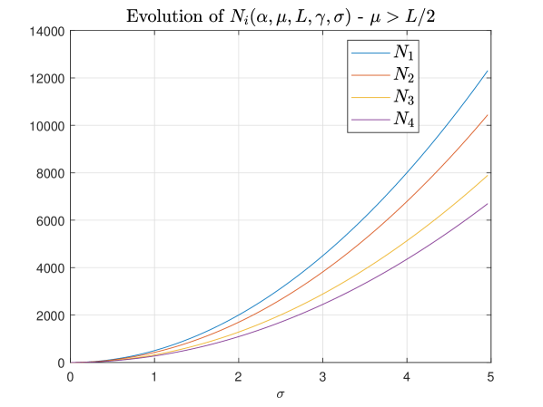
Figure 9: Evolution of $N_{i}(\alpha,\mu,L,\gamma,\sigma)$ w.r.t $\sigma$ for scenario $\mu>L/2$; $\gamma=3/2$, $\mu=1$, $L=3/2$, $\alpha=\frac{\mu+\gamma+\sqrt{(\mu-\gamma)^{2}+4\gamma L}}{L-\mu}$.

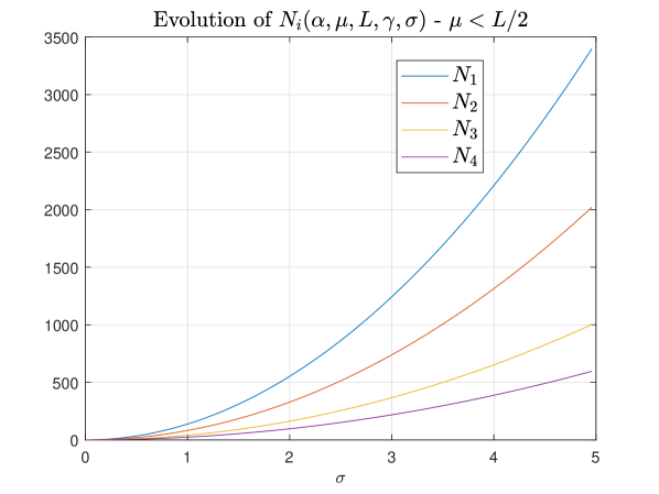
Figure 10: Evolution of $N_{i}(\alpha,\mu,L,\gamma,\sigma)$ w.r.t $\sigma$ for scenario $\mu<L/2$; $\gamma=3/2$, $\mu=1$, $L=3$, $\alpha=\frac{\mu+\gamma+\sqrt{(\mu-\gamma)^{2}+4\gamma L}}{L-\mu}$.

A.1.4 Extension to $n$-dimensional case

In this section, we show that we can easily extend the results obtained for the $2$-dimensional case in Section A.1.1, Section A.1.2 and Section A.1.3 to the $n$-dimensional case with $n>2$. Let us start by recalling that for NAG transformation (7), the general SDE’s system to solve for the quadratic case is:

$$\dot{y}(t)=\begin{bmatrix}-I_{n\times n}&I_{n\times n}\\ 1/\gamma(\mu I_{n\times n}-A)&-\mu/\gamma I_{n\times n}\end{bmatrix}y(t)+\begin{bmatrix}0_{n\times 1}\\ \frac{dZ}{dt}\end{bmatrix},\quad t>0.$$ (49)

Let recall that $y=(x,v)$ with $x,v\in\mathbb{R}^{n}$, let $n$ be even and let consider the permutation matrix $P$ associated to permutation indicator $\pi$ given here-under in two-line form: $\begin{aligned} \pi=\left[\begin{array}[]{ccccccc|cccccc}(1&2)&(3&4)&\cdots&(n-1&n)&(n+1&n+2)&\cdots&(2n-1&2n)\\ (2*1-1&2*1)&(2*3-1&2*3)&\cdots&(2n-3&2n-2)&(3&4)&\cdots&(2n-1&2n)\end{array}\right]\end{aligned}$ where the bottom second-half part of $\pi$ corresponds to the complementary of the bottom first half w.r.t. to the set $\{1,2,...,2n\}$ in the increasing order. For avoiding ambiguities, the ones element of $P$ are at indices $(\pi(1,j),\pi(2,j))$ for $1\leq j\leq 2n$. For such convention and since permutation matrix $P$ associated to indicator $\pi$ is orthogonal matrix, equation 49 can be equivalently written as follows:

$$\dot{y}(t)=PP^{T}\begin{bmatrix}-I_{n\times n}&I_{n\times n}\\ 1/\gamma(\mu I_{n\times n}-A)&-\mu/\gamma I_{n\times n}\end{bmatrix}PP^{T}y(t)+\begin{bmatrix}0_{n\times 1}\\ \dot{Z}\end{bmatrix},$$ (50)

$$\equiv P^{T}\dot{y}(t)=P^{T}\begin{bmatrix}-I_{n\times n}&I_{n\times n}\\ 1/\gamma(\mu I_{n\times n}-A)&-\mu/\gamma I_{n\times n}\end{bmatrix}PP^{T}y(t)+P^{T}\begin{bmatrix}0_{n\times 1}\\ \dot{Z}\end{bmatrix},$$

Since we assumed w.l.o.g. $A=\text{diag}(\lambda_{1},\ldots,\lambda_{n})$ with $\mu=\lambda_{1}\leq\ldots\leq\lambda_{n}=L$, one can easily see that Equation equation 50 has the structure:

which boils down to $m=\frac{n}{2}$ independent 2-dimensional SDE’s systems where $A_{i}=\text{diag}(\lambda_{2i-1},\lambda_{2i})$ with $1\leq i\leq m$ such that $\lambda_{1}=\mu$ and $\lambda_{n}=L$.

Therefore, the $m$ SDE’s systems can be studied and theoretically solved independently with the schemes and the associated step sizes presented in previous sections. However, in practice, we will use a unique and general step size $\alpha$ to tackle the full SDE’s system 49.

Let now use the "decoupled" structure given in equation 51 to come up with a general step size that will ensure the convergence of each system and hence the convergence of the full original system given in equation 49. Let us denote by $\alpha_{i}$ the step size for the $i$-th SDE’s system with $1\leq i\leq m=n/2$ minimizing the spectral radius of the system at hand. For convenience, let us consider the case $\gamma>\mu$, we apply the same method as detailed in Section A.1.1 and Section A.1.2 to compute the expression of $\alpha_{i}$ that minimizes $\rho(E_{i}(\alpha))$, we obtain:

$$\alpha_{i}=\frac{\mu+\gamma+\sqrt{(\mu-\gamma)^{2}+4\gamma\lambda_{2i}}}{\lambda_{2i}-\mu}$$ (52)

Finally, in Theorem 1, we show that choosing $\alpha_{c}:=\alpha=\frac{\mu+\gamma+\sqrt{(\mu-\gamma)^{2}+4\gamma L}}{L-\mu}$ ensures the convergence of NAG-GS method used to solve the SDE’s system 49 in the $n$-dimensional case for $n>2$. Theorem 1 is enunciated in Section 2.3 in the main text and the proof is given here-under.

Proof.

First, we recall that Lemma 3 in Section A.1.3 provides the proof for the asymptotic convergence of NAG-GS method for $n=2$ when choosing $\alpha:=\alpha_{c}=\frac{\mu+\gamma+\sqrt{(\mu-\gamma)^{2}+4\gamma L}}{L-\mu}$ for the case $\gamma>\mu$. In particular, it is shown that the spectral radius of the iteration matrix $\rho(E(\alpha_{c}))$ is strictly lower than 1 under consistent assumptions with the ones of Theorem 1 (see Lemma 3 for more details). The following steps of the proof show that choosing $\alpha_{c}$ also leads to the asymptotic convergence of NAG-GS method for $n>2$.

To do so, let us start by considering, w.l.o.g., the SDE’s system in the form given by equation 51 and let $\alpha_{i}=\frac{\mu+\gamma+\sqrt{(\mu-\gamma)^{2}+4\gamma\lambda_{2i}}}{\lambda_{2i}-\mu}$ be the step size (given in Equation 52) selected for solving the $i$-th SDE’s system with $1\leq i\leq m=n/2$, minimizing $\rho(E_{i}(\alpha))$, that is the spectral radius of the associated iteration matrix $E_{i}$. The result of Lemma 3 can be directly extended for each independent 2-dimensional SDE’s system, in particular showing that $\rho(E_{i}(\alpha_{i}))<1$ for $1\leq i\leq m=n/2$.

Therefore, to prove the convergence of the NAG-GS method by choosing a single step size $\alpha$ such that $0<\alpha\leq\frac{\mu+\gamma+\sqrt{(\mu-\gamma)^{2}+4\gamma L}}{L-\mu}$, it suffices to show that:

$$\alpha=\frac{\mu+\gamma+\sqrt{(\mu-\gamma)^{2}+4\gamma L}}{L-\mu}\leq\underset{1\leq i\leq m=n/2}{\text{min}}\alpha_{i}$$ (53)

For proving that equation 53 holds, it sufficient to show that for any $\lambda$ such that $0<\mu\leq\lambda\leq L<\infty$ we have:

$$\frac{\mu+\gamma+\sqrt{(\mu-\gamma)^{2}+4\gamma L}}{L-\mu}\leq\frac{\mu+\gamma+\sqrt{(\mu-\gamma)^{2}+4\gamma\lambda}}{\lambda-\mu}.$$ (54)

which is equivalent to showing:

$$\frac{\mu+\gamma+\sqrt{(\mu-\gamma)^{2}+4\gamma L}}{L-\mu}-\frac{\mu+\gamma+\sqrt{(\mu-\gamma)^{2}+4\gamma\lambda}}{\lambda-\mu}\leq 0$$ (55)

$$\equiv \gamma(\frac{1}{L-\mu}-\frac{1}{\lambda-\mu})+\mu(\frac{1}{L-\mu}-\frac{1}{\lambda-\mu})+\frac{\sqrt{(\mu-\gamma)^{2}+4\gamma L}}{L-\mu}-\frac{\sqrt{(\mu-\gamma)^{2}+4\gamma\lambda}}{\lambda-\mu}\leq 0$$

Since $0<\mu\leq\lambda\leq L<\infty$ by hypothesis, one can easily show that first two terms of the last inequality are negative. It remains to show that:

$$\frac{\sqrt{(\mu-\gamma)^{2}+4\gamma L}}{L-\mu}-\frac{\sqrt{(\mu-\gamma)^{2}+4\gamma\lambda}}{\lambda-\mu}\leq 0$$ (56)

$$\equiv (-\gamma^{2}-4\gamma\lambda+2\gamma\mu-\mu^{2})L^{2}+(4\gamma\lambda^{2}+2\gamma^{2}\mu+2\mu^{3})L+$$

$$\gamma^{2}\lambda^{2}-2\gamma^{2}\lambda\mu-2\gamma\lambda^{2}\mu+\lambda^{2}\mu^{2}-2\lambda\mu^{3}\leq 0$$

Note that we can easily show that the coefficient of $L^{2}$ is negative, hence last inequality is satisfied as soon as $L\leq\frac{-\gamma^{2}\lambda+2\gamma^{2}\mu+2\gamma\lambda\mu-\lambda\mu^{2}+2\mu^{3}}{\gamma^{2}+4\gamma\lambda-2\gamma\mu+\mu^{2}}$ or $L\geq\lambda$. The latter condition is satisfied by hypothesis, this concludes the proof.

Note that one can check that $\frac{-\gamma^{2}\lambda+2\gamma^{2}\mu+2\gamma\lambda\mu-\lambda\mu^{2}+2\mu^{3}}{\gamma^{2}+4\gamma\lambda-2\gamma\mu+\mu^{2}}\leq\lambda$. ∎

The theoretical results derived in these sections along with the key insights are validated in Section A.1.5 through numerical experiments conducted for the NAG-GS method in the quadratic case.

A.1.5 Numerical tests for quadratic case

In this section, we report some simple numerical tests for the NAG-GS method (Algorithm 1) used to tackle the accelerated SDE’s system given in (11) where:

• the objective function is $f(x)=(x-ce)^{T}A(x-ce)$ with $A\in\mathbb{S}^{3}_{+}$, $e$ a all-ones vector of dimension 3 and $c$ a positive scalar. For such a strongly convex setting, since the feasible set is $V=\mathbb{R}^{3}$, the minimizer $\arg\min f$ uniquely exists and is simply equal to $ce$; it will be denoted further by $x^{\star}$. The matrix $A$ is generated as follows: $A=QAQ^{-1}$ where matrix $D$ is a diagonal matrix of size 3 and $Q$ is a random orthogonal matrix. This test procedure allows us to specify the minimum and maximum eigenvalues of $A$ that are respectively $\mu$ and $L$ and hence it allows us to consider the two scenarios discussed in Section A.1.1, that are $\mu>L/2$ and $\mu<L/2$.

• The noise volatility $\sigma$ is set to 1, we report that this corresponds to a significant level of noise.

• Initial parameter $\gamma_{0}$ is set to $\mu$.

• Different values for the step size $\alpha$ will be considered in order to empirically demonstrate the optimal choice $\alpha_{c}$ in terms of contraction rate, but also validate the critical values for step size in the case $\mu<L/2$ and, finally, highlight the effect of the step size in terms of scattering of the final iterates generated by NAG-GS around the minimizer of $f$.

From a practical point of view, we consider $m=200000$ points. For each of them, the NAG-GS method is run for a maximum number of iterations to reach the stationarity, and the initial state $x_{0}$ is generated using normal Gaussian distribution. Since $f(x)$ is a quadratic function, it is expected that the points will converge to some Gaussian distribution around the minimizer $x^{\star}=ce$. Furthermore, since the initial distribution is also Gaussian, then it is expected that the intermediate distributions (at each iteration of the NAG-GS method) are Gaussian as well. Therefore, in order to quantify the rate of convergence of the NAG-GS method for different values of step size, we will monitor $\|\bar{x}^{k}-x^{\star}\|$, that is the distance between the empirical mean of the distribution at iteration $k$ and the minimizer $x^{\star}$ of $f$.

Figures 11 and 12 respectively show the evolution of $\|\bar{x}^{k}-x^{\star}\|$ along iteration and the final distribution of points obtained by NAG-GS at stationarity for the scenario $\mu>L/2$, for the latter the points are projected onto the three planes to have a full visualization. As expected by the theory presented in Section A.1.3, there is no critical $\alpha$, hence one may choose arbitrary large values for step size while the NAG-GS method still converges. Moreover, the choice of $\alpha=\alpha_{c}$ gives the highest rate of convergence. Finally, one can observe that the distribution of limit points tightens more and more around the minimizer $x^{\star}$ of $f$ as the chosen step increases, as expected by the analysis of Figure 7. Hence, one may choose a very large step size $\alpha$ so that the limit points converge to $x^{\star}$ almost surely but at a cost of a (much) slower convergence rate. Here comes the tradeoff between the convergence rate and the limit points scattering.

Finally, Figures 13 and 14 provide similar results for the scenario $\mu<L/2$. The theory outlined in Section A.1.3 and Section A.1.4 predicts a critical value of $\alpha$ that indicates when the convergence of NAG-GS is destroyed in such a scenario. In order to illustrate this gradually, different values of $\alpha$ have been chosen within the set $\{\alpha_{c},\alpha_{c}/2,(\alpha_{c}+\alpha_{\text{crit}})/2,0.98\alpha_{\text{crit}}\}$. First, one can observe that the choice of $\alpha=\alpha_{c}$ gives again the highest rate of convergence, see Figure 13. Moreover, one can clearly see that for $\alpha\rightarrow\alpha_{\text{crit}}$, the convergence starts to fail and the spreading of the limit points tends to infinity. We report that for $\alpha=\alpha_{\text{crit}}$, NAG-GS method diverges. Again, these numerical results are fully predicted by the theory derived in previous sections.

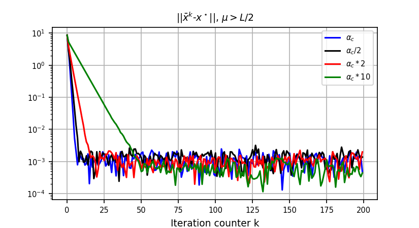
Figure 11: Evolution of $\|\bar{x}^{k}-x^{\star}\|$ along iteration for the scenario $\mu>L/2$; $c=5$, $\gamma=\mu=1$, $L=1.9$ and $\sigma=1$ for $\alpha\in\{\alpha_{c},\alpha_{c}/2,2\alpha_{c},10\alpha_{c}\}$ with $\alpha_{c}=\frac{2\mu+2\sqrt{\mu L}}{L-\mu}=5.29$.

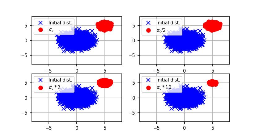
(a) Projection in $XY$ plane.

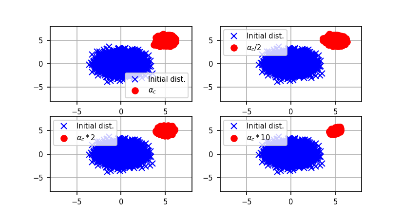
(b) Projection in $YZ$ plane.

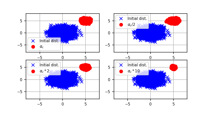
(c) Projection in $XZ$ plane.

Figure 12: Initial (blue crosses) and final (red circles) distributions of points generated by the NAG-GS method for the scenario $\mu>L/2$; $c=5$, $\gamma=\mu=1$, $L=1.9$ and $\sigma=1$ for $\alpha\in\{\alpha_{c},\alpha_{c}/2,2\alpha_{c},10\alpha_{c}\}$ with $\alpha_{c}=\frac{2\mu+2\sqrt{\mu L}}{L-\mu}=5.29$.

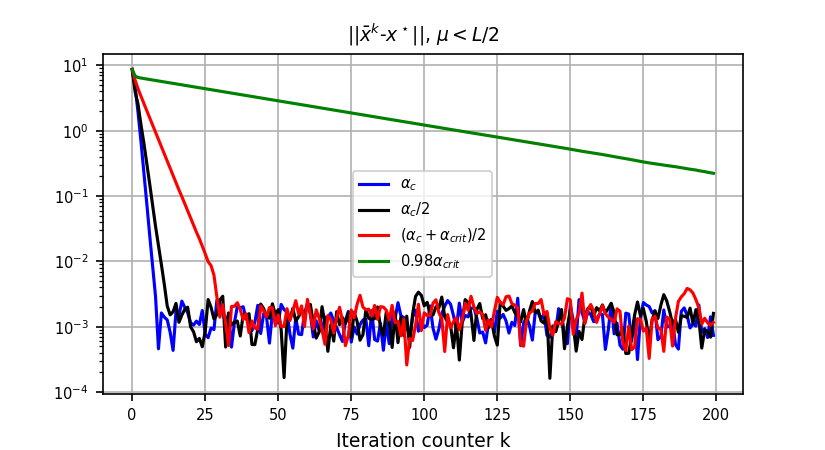
Figure 13: Evolution of $\|\bar{x}^{k}-x^{\star}\|$ along iteration for the scenario $\mu<L/2$; $c=5$, $\gamma=\mu=1$, $L=3$ and $\sigma=1$ for $\alpha\in\{\alpha_{c},\alpha_{c}/2,(\alpha_{c}+\alpha_{\text{crit}})/2,0.98\alpha_{\text{crit}}\}$ with $\alpha_{c}=\frac{2\mu+2\sqrt{\mu L}}{L-\mu}=2.73$ and $\alpha_{\text{crit}}=\frac{\mu+\gamma+\sqrt{\gamma^{2}-6\gamma\mu+\mu^{2}+4\gamma L}}{L-2\mu}=4.83$.

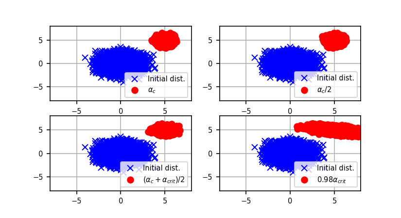
(a) Projection in $XY$ plane.

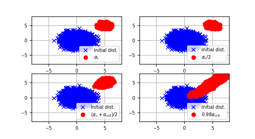
(b) Projection in $YZ$ plane.

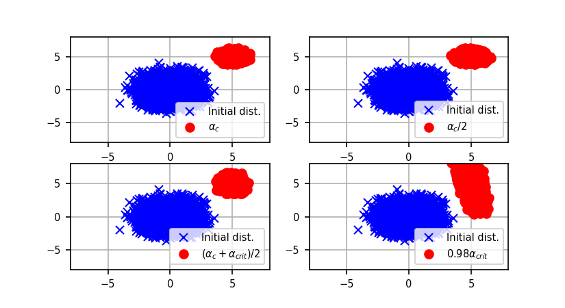
(c) Projection in $XZ$ plane.

Figure 14: Initial (blue crosses) and final (red circles) distributions of points generated by the NAG-GS method for scenario $\mu<L/2$; $c=5$, $\gamma=\mu=1$, $L=3$ and $\sigma=1$ for $\alpha\in\{\alpha_{c},\alpha_{c}/2,(\alpha_{c}+\alpha_{\text{crit}})/2,0.98\alpha_{\text{crit}}\}$ with $\alpha_{c}=\frac{2\mu+2\sqrt{\mu L}}{L-\mu}=2.73$ and $\alpha_{\text{crit}}=\frac{\mu+\gamma+\sqrt{\gamma^{2}-6\gamma\mu+\mu^{2}+4\gamma L}}{L-2\mu}=4.83$.

A.2 Fully-implicit scheme

In this section, we present an iterative method based on the NAG transformation $G_{NAG}$ (7) along with a fully implicit discretization to tackle (4) in the stochastic setting, the resulting method shall be referred to as "NAG-FI" method. We propose the following discretization for (6) perturbated with noise; given step size $\alpha_{k}>0$:

$$\begin{split}&\frac{x_{k+1}-x_{k}}{\alpha_{k}}=v_{k+1}-x_{k+1},\\ &\frac{v_{k+1}-v_{k}}{\alpha_{k}}=\frac{\mu}{\gamma_{k}}(x_{k+1}-v_{k+1})-\frac{1}{\gamma_{k}}Ax_{k+1}+\sigma\frac{W_{k+1}-W_{k}}{\alpha_{k}}.\end{split}$$ (57)

As done for the NAG-GS method, from a practical point of view, we will use $W_{k+1}-W_{k}=\Delta W_{k}=\sqrt{\alpha_{k}}\eta_{k}$ where $\eta_{k}\sim\mathcal{N}(0,1)$, by the properties of the Brownian motion.

In the quadratic case, that is $f(x)=\frac{1}{2}x^{\top}Ax$, solving equation 57 is equivalent to solve:

$$\begin{bmatrix}x_{k}\\ v_{k}+\sigma\sqrt{\alpha_{k}}\eta_{k}\end{bmatrix}=\begin{bmatrix}(1+\alpha_{k})I&-\alpha_{k}I\\ \frac{\alpha_{k}}{\gamma_{k}}(A-\mu I)&(1+\frac{\alpha_{k}\mu}{\gamma_{k}})I\end{bmatrix}\begin{bmatrix}x_{k+1}\\ v_{k+1}\end{bmatrix}$$ (58)

where $\eta_{k}\sim\mathcal{N}(0,1)$. Furthermore, ODE (8) from the main text is again discretized implicitly:

$$\frac{\gamma_{k+1}-\gamma_{k}}{\alpha_{k}}=\mu-\gamma_{k+1},\quad\gamma_{0}>0.$$ (59)

As done for NAG-GS method, heuristically, for general $f\in\mathcal{S}^{1,1}_{L,\mu}$ with $\mu\geq 0$, we just replace $Ax_{k+1}$ in equation 57 with $\nabla f(x_{k+1})$ and obtain the following NAG-FI scheme:

$$\begin{split}&\frac{x_{k+1}-x_{k}}{\alpha_{k}}=v_{k+1}-x_{k+1},\\ &\frac{v_{k+1}-v_{k}}{\alpha_{k}}=\frac{\mu}{\gamma_{k}}(x_{k+1}-v_{k+1})-\frac{1}{\gamma_{k}}\nabla f(x_{k+1})+\sigma\frac{W_{k+1}-W_{k}}{\alpha_{k}}.\end{split}$$ (60)

From the first equation, we get $v_{k+1}=\frac{x_{k+1}-x_{k}}{\alpha_{k}}+x_{k+1}$ that we substitute within the second equation, we obtain:

$$x_{k+1}=\frac{v_{k}+\tau_{k}x_{k}-\frac{\alpha_{k}}{\gamma_{k}}\nabla f(x_{k+1})+\sigma\sqrt{\alpha_{k}}\eta_{k}}{1+\tau_{k}}$$ (61)

with $\tau_{k}=1/\alpha_{k}+\mu/\gamma_{k}$.

Computing $x_{k+1}$ is equivalent to computing a fixed point of the operator given by the right-hand side of equation 61. Hence, it is also equivalent to finding the root of the function:

$$g(u)=u-\left(\frac{v_{k}+\tau_{k}x_{k}-\frac{\alpha_{k}}{\gamma_{k}}\nabla f(u)+\sigma\sqrt{\alpha_{k}}\eta_{k}}{1+\tau_{k}}\right)$$ (62)

with $g:\mathbb{R}^{n}\rightarrow\mathbb{R}^{n}$. In order to compute the root of this function, we consider a classical Newton-Raphson procedure detailed in Algorithm 2.

Algorithm 2 Newton-Raphson method

0:  Choose the point $u_{0}\in\mathbb{R}^{n}$, some $\alpha_{k},\gamma_{k},\tau_{k}>0$.

  for $i=0,1,\ldots$ do

     Compute $J_{g}(u_{i})=I_{n}+\frac{\alpha_{k}}{\gamma_{k}(1+\tau_{k})}\nabla^{2}f(u_{i})$

     Compute $g(u_{i})$ using equation 62

     Set $u_{i+1}=u_{i}-[J_{g}(u_{i})]^{-1}g(u_{i})$

  end for

In Algorithm 2, $J_{g}(.)$ denotes the Jacobian operator of function $g$ equation 62 w.r.t. $u$, $I_{n}$ denotes the identity matrix of size $n$ and $\nabla^{2}f$ denotes the Hessian matrix of objective function $f$. Please note that the iterative method outlined in Algorithm 2 exhibits a connection to the family of second-order methods called the Levenberg-Marquardt algorithm Levenberg (1944); Marquardt (1963) applied to the unconstrained minimization problem $\min_{x\in\mathbb{R}^{n}}f(x)$ for a twice-differentiable function $f$. Finally, Algorithm 3 summarizes the NAG-FI method.

Algorithm 3 NAG-FI Method

0:  Choose the point $x_{0}\in\mathbb{R}^{n}$, set $v_{0}=x_{0}$, some $\sigma\geq 0$, $\mu\geq 0,\gamma_{0}>0$.

  for $k=0,1,\ldots$ do

     Sample $\eta_{k}\sim\mathcal{N}(0,1)$

     Choose $\alpha_{k}>0$

     Set $\gamma_{k+1}:=\frac{\gamma_{k}+\alpha_{k}\mu}{1+\alpha_{k}}$

     Set $\tau_{k+1}=1/\alpha_{k}+\mu/\gamma_{k+1}$

     Compute the root $u$ of equation 62 by using Algorithm 2

     Set $x_{k+1}=u$

  end for

By following a similar stability analysis as the one performed for NAG-GS, one can show that this method is unconditionally A-stable as expected by the theory of implicit schemes. In particular, one can show that eigenvalues of the iterations matrix are positive decreasing functions w.r.t. step size $\alpha$, allowing then the choice of any positive value for $\alpha$. Similarly, one can show that the eigenvalues of the covariance matrix at stationarity associated with the NAG-FI method are decreasing functions w.r.t. $\alpha$ that tend to 0 as soon as $\alpha\rightarrow\infty$. It implies that Algorithm 3 is theoretically able to generate iterates that converge to $\arg\min f$ almost surely, even in the stochastic setting with the potentially quadratic rate of converge. This theoretical result is quickly highlighted in Figure 15 that shows the final distribution of points generated by NAG-FI once used in test setup detailed in Section A.1.5, in the most interesting and critical scenario $\mu<L/2$. As expected, $\alpha$ can be chosen as large as desired, we choose here $\alpha=1000\alpha_{c}$. Moreover, for increasing $\alpha$, the final distributions of points are more and more concentrated around $x^{*}$.

Therefore, the NAG-FI method constitutes a good basis for deriving efficient second-order methods for tackling stochastic optimization problems, which is hard to find in the current SOTA. Indeed, second-order methods and more generally some variants of preconditioned gradient methods have recently been proposed and used in the deep learning community for the training of NN for instance. However, it appears that there is limited empirical success for such methods when used for training NN when compared to well-tuned Stochastic Gradient Descent schemes, see for instance Botev et al. (2017); Zeiler (2012). To the best of our knowledge, no theoretical explanations have been brought to formally support these empirical observations. This will be part of our future research directions.

Besides these nice preliminary theoretical results and numerical observations for small dimension problems, there is a limitation of the NAG-FI method that comes from the numerical feasibility for computing the root of the non-linear function equation 62 that can be very challenging in practice. We will try to address this issue in future works.

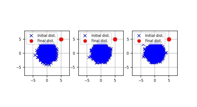
Figure 15: Projection onto $XY$, $YZ$, and $XZ$ planes (from left to right) of initial (blue crosses) and final (red circles) distributions of points generated by NAG-FI method - scenario $\mu<L/2$; $c=5$, $\gamma=\mu=1$, $L=3$ and $\sigma=1$ for $\alpha=1000\alpha_{c}$ with $\alpha_{c}=\frac{2\mu+2\sqrt{\mu L}}{L-\mu}=2.73$.

Appendix B Convergence to the stationary distribution

Another way to study the convergence of the proposed algorithms is to consider the Fokker-Planck equation for the density function $\rho(t,x)$. We will consider the simple case of the scalar SDE for the stochastic gradient flow (similarly as in (11)). Here $f:\mathbb{R}\to\mathbb{R}$:

$$dx=-\nabla f(x)dt+dZ=-\nabla f(x)dt+\sigma dW,\quad x(0)\sim\rho(0,x).$$

It is well known, that the density function for $x(t)\sim\rho(t,x)$ satisfies the corresponding Fokker-Planck equation:

$$\dfrac{\partial\rho(t,x)}{\partial t}=\nabla\left(\rho(t,x)\nabla f(x)\right)+\frac{\sigma^{2}}{2}\Delta\rho(t,x)$$ (63)

For the equation 63 one could write down the stationary (with $t\to\infty$) distribution

$$\rho^{*}(x)=\lim_{t\to\infty}\rho(t,x)=\dfrac{1}{Z}\exp\left(-\frac{2}{\sigma^{2}}f(x)\right),\quad Z=\int\limits_{x\in V}\exp\left(-\frac{2}{\sigma^{2}}f(x)\right)dx.$$ (64)

It is useful to compare different optimization algorithms in terms of convergence in the probability space because it allows us to study the methods in the non-convex setting. We have to address two problems with this approach. Firstly, we need to specify some distance functional between current distribution $\rho_{t}=\rho(t,x)$ and stationary distribution $\rho^{*}=\rho^{*}(x)$. Secondly, we do not need to have access to the densities $\rho_{t},\rho^{*}$ themselves.

For the first problem, we will consider the following distance functionals between probability distributions in the scalar case:

• Kullback-Leibler divergence. Several studies dedicated to convergence in probability space are available Arnold et al. (2001); Chewi et al. (2020); Lambert et al. (2022). We used the approach proposed in Pérez-Cruz (2008) to estimate KL divergence between continuous distributions based on their samples.

• Wasserstein distance. Wasserstein distance is relatively easy to compute for scalar densities. Also, it was shown, that the stochastic gradient process with a constant learning rate is exponentially ergodic in the Wasserstein sense Latz (2021).

• Kolmogorov-Smirnov statistics. We used the two-sample Kolmogorov-Smirnov test for goodness of fit.

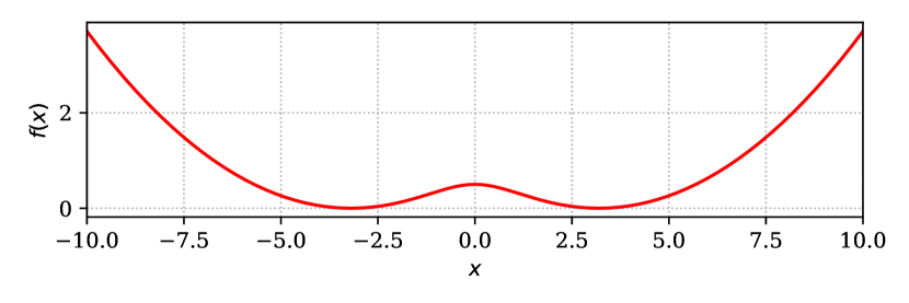
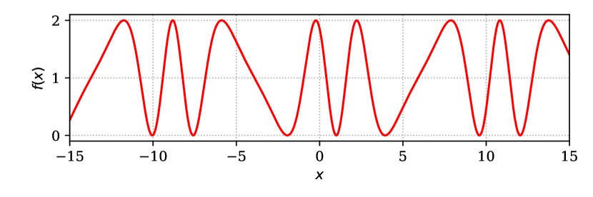
(a) Two pits function.
$f_{1}(x)=\frac{1}{50}\left(2\log\left(\cosh(x)\right)-5\right)^{2}$

(b) Frequently modulated sin function.
$f_{2}(x)=\cos\left(1.6x+\frac{5}{3}\sin(0.64x)-\pi\right)$

Figure 16: Non convex scalar functions to test

To the best of our knowledge, the explicit formula for the stationary distribution of Fokker-Planck equations for the ASG SDE (11) remains unknown. That is why we have decided to get samples from the empirical stationary distributions using Euler-Maruyama integration Maruyama (1955) with a small enough step size of corresponding SDE with a bunch of different independent initializations.

We tested two functions, which are presented in Figure 16. We initially generated $100$ points uniformly in the function domain. Then we independently solved the initial value problem (9) for each of them with Maruyama (1955). Results of the integration are presented in Figure 17. One can see, that in the relatively easy case (Figure 16), NAG-GS converges faster, than gradient flow to its stationary distribution, see Figure 17(a). At the same time, in the hard case (Figure 16), NAG-GS is more robust to the large step size, see Figure 17(b).

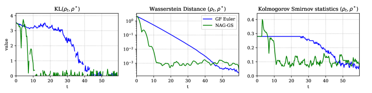
(a) Results for $f_{1}(x)$. $\alpha=8*10^{-3},\sigma=10^{-3},\mu=\frac{1}{33}$

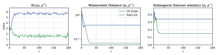
(b) Results for $f_{2}(x)$. $\alpha=1.5,\sigma=10^{-2},\mu=1$

Figure 17: Convergence in probabilities of Euler integration of Gradient Flow (GF Euler) and NAG-GS for the non-convex scalar problems.

Appendix C Additional insights

In this section, we provide additional experimental details. In particular, we discuss a little bit more our experimental setup and give some insights about NAG-GS as well.

Our computational resources are limited to a single Nvidia DGX-1 with 8 GPUs Nvidia V100. Almost all experiments were carried out on a single GPU. The only exception is for the training of ResNet50 on ImageNet which used all 8 GPUs.

C.1 Phase diagrams

In Section C.4 we mentioned that the lowest eigenvalues $\mu$ of approximated Hessian matrices evaluated during the training of the ResNet-20 model were negative. Furthermore, our theoretical analysis of NAG-GS in the convex case includes some conditions on the optimizer parameters $\alpha$, $\gamma$, and $\mu$. In particular, it is required that $\mu>0$ and $\gamma\geq\mu$. In order to bring some insights about these remarks in the non-convex setting and inspired by Velikanov et al. (2022), we experimentally study the convergence regions of NAG-GS and sketch out the phase diagrams of convergence for different projection planes, see Figure 18.

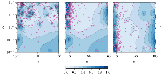
Figure 18: Landscapes of classification error for ResNet-20 model trained on CIFAR-10 with NAG-GS after projections onto $\alpha-\gamma$, $\alpha-\mu$ and $\gamma-\mu$ planes (from left to right). Hyperparameter optimization algorithm samples learning rate $\alpha$ from $[10^{-2},\,10^{2}]$, factor $\gamma$ from $[10^{-2},\,10^{2}]$, and factor $\mu$ from $[-10,90]$. Hyperparameters $\alpha$ and $\gamma$ are sampled from log-uniform distribution, and hyperparameter $\mu$ is sampled from a uniform distribution.

We consider the same setup as in Section 3.4 in the main text, a paragraph about the ResNet-20 model, and use hyper-optimization library Optuna Akiba et al. (2019). Our preliminary experiments on RoBERTa show that $\alpha$ should be of magnitude $10^{-1}$. With the estimate of the Hessian spectrum of ResNet-20, we define the following search space

$$\alpha\sim\mathrm{LogUniform}(10^{-2},10^{2}),\quad\gamma\sim\mathrm{LogUniform}(10^{-2},10^{2}),\quad\mu\sim\mathrm{Uniform}(-10,100).$$

We sample a fixed number of triples and train the ResNet-20 model on CIFAR-10. The objective function is a top-1 classification error.

We report that there is a convergence almost everywhere within the projected search space onto $\alpha$-$\gamma$ plane (see Figure 18). The analysis of projections onto $\alpha$-$\mu$ and $\gamma$-$\mu$ planes brings different conclusions: there are regions of convergence for negative $\mu$ for some $\alpha<\alpha_{th}$ and $\gamma>\gamma_{th}$. Also, there is a subdomain of negative $\mu$ comparable to a domain of positive $\mu$ in the sense of the target metrics. Moreover, the majority of sampled points are located in the vicinity of the band $\lambda_{\min}<\mu<\lambda_{\max}$.

C.2 Implementation Details

In our work, we implemented NAG-GS in PyTorch Paszke et al. (2017) and JAX Bradbury et al. (2018); Babuschkin et al. (2020). Both implementations are used in our experiments and available online. According to Algorithm 1, the size of the NAG-GS state equals to number of optimization parameters which makes NAG-GS comparable to SGD with momentum. It is worth noting that Adam-like optimizers have a twice larger state than NAG-GS. The arithmetic complexity of NAG-GS is linear $O(n)$ in the number of parameters. Table 6 shows a comparison of the computational efficiency of common optimizers used in practice. Although forward pass and gradient computations usually give the main contribution to the training step, there is a setting where the efficiency of gradient updates is important (e.g. batch size or a number of intermediate activations are small with respect to a number of parameters).

Table 6: The comparison of a single step duration for different optimizers on ResNet-20 on CIFAR-10. Adam-like optimizers have in twice larger state than SGD with momentum or NAG-GS.

Optimizer	Mean, s	Variance, s	Rel. Mean	Rel. Variance
SGD	0.458	0.008	1.0	1.0
NAG-GS	1.648	0.045	3.6	5.5
SGD-M	3.374	0.042	7.4	5.2
SGD-MW	3.512	0.037	17.7	4.7
AdamW	5.208	0.102	11.4	12.6
Adam	7.919	0.169	17.3	20.8

C.3 Updatable Scaling Factor $\gamma$

According to the theory of NAG-GS optimizer presented in Section 2, the scaling factor $\gamma$ decays exponentially fast to $\mu$ and, in the case $\gamma_{0}=\mu$, $\gamma$ remains constant along iterations. So, a natural question arises: is the update on $\gamma$ necessary? Our experiments confirm that scaling factor $\gamma$ should be updated accordingly to Algorithm 1, even in this highly non-convex setting, in order to get better metrics on test sets.

We use an experimental setup for ResNet-20 from Section 3.4 in the main text and search for hyperparameters for NAG-GS with updatable $\gamma$ and with constant one. Common hyper-optimization library Optuna Akiba et al. (2019) is used with a budget of 160 iterations to sample NAG-GS parameters. Figure 19 plots the evolution of the best score value along optimization time.

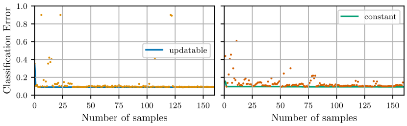
Figure 19: The best acc@1 on test set for updatable and fixed scaling factor $\gamma$ during hyperoptimization. NAG-GS with updatable $\gamma$ gives more frequently better results than the ones obtained with constant $\gamma$.

C.4 Non-Convexity and Hessian Spectrum

Theoretical analysis of NAG-GS highlights the importance of the smallest eigenvalue of the Hessian matrix for convex and strongly convex functions. Unfortunately, the objective functions usually considered for the training of neural networks are not convex. In this section, we try to address this issue. The smallest model in our experimental setup is ResNet-20. However, we cannot afford to compute exactly the Hessian matrix since ResNet-20 has almost 300k parameters. Instead, we use Hessian-vector product (HVP) $H(x)$ and apply matrix-free algorithms for finding the extreme eigenvalues. We estimate the extreme eigenvalues of the Hessian spectrum with power iterations (PI) along with Rayleigh quotient (RQ) Golub & van Loan (2013). PI is used to get a good initial vector which is used later in the optimization of RQ. In order to get a more useful initial vector for the estimation of the smallest eigenvalue, we apply the spectral shift $H(x)-\lambda_{\max}x$ and use the corresponding eigenvector.

Figure 20 shows the extreme eigenvalues of ResNet-20 Hessian at the end of each epoch for the batch size 256 in the same setup as in Section 3.4 in the main text. The largest eigenvalue is strictly positive while the smallest one is negative and usually oscillates around $-1$. It turns out that there is an island of hyperparameters in the vicinity of that $\mu$. We report that training ResNet-20 with hyperparameters included in this island gives good target metrics. The domain of negative momenta is non-conventional and not well understood, to the best of our knowledge. Moreover, there are no theoretical guarantees for NAG-GS in the non-convex case and negative $\mu$. However, Velikanov et al. (2022) reports the existence of regions of convergence for SGD with negative momentum, which supports our observations. The theoretical aspects of these observations will be studied in future work.

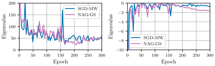
Figure 20: Evolution of the extreme eigenvalues (the largest and the smallest ones) during training ResNet-20 on CIFAR-10 with the NAG-GS optimizer.

References

- Akiba et al. (2019) Takuya Akiba, Shotaro Sano, Toshihiko Yanase, Takeru Ohta, and Masanori Koyama. Optuna: A next-generation hyperparameter optimization framework. In Proceedings of the 25rd ACM SIGKDD International Conference on Knowledge Discovery and Data Mining, 2019.
- Arnold et al. (2001) Anton Arnold, Peter Markowich, Giuseppe Toscani, and Andreas Unterreiter. On convex sobolev inequalities and the rate of convergence to equilibrium for fokker-planck type equations. 2001.
- Attouch et al. (2019) Hedy Attouch, Zaki Chbani, and Hassan Riahi. Fast proximal methods via time scaling of damped inertial dynamics. SIAM Journal on Optimization, 29(3):2227–2256, 2019.
- Babuschkin et al. (2020) Igor Babuschkin, Kate Baumli, Alison Bell, Surya Bhupatiraju, Jake Bruce, Peter Buchlovsky, David Budden, Trevor Cai, Aidan Clark, Ivo Danihelka, Claudio Fantacci, Jonathan Godwin, Chris Jones, Ross Hemsley, Tom Hennigan, Matteo Hessel, Shaobo Hou, Steven Kapturowski, Thomas Keck, Iurii Kemaev, Michael King, Markus Kunesch, Lena Martens, Hamza Merzic, Vladimir Mikulik, Tamara Norman, John Quan, George Papamakarios, Roman Ring, Francisco Ruiz, Alvaro Sanchez, Rosalia Schneider, Eren Sezener, Stephen Spencer, Srivatsan Srinivasan, Luyu Wang, Wojciech Stokowiec, and Fabio Viola. The DeepMind JAX Ecosystem, 2020. URL http://github.com/deepmind.
- Biewald (2020) Lukas Biewald. Experiment tracking with weights and biases, 2020. URL https://www.wandb.com/. Software available from wandb.com.
- Bossard et al. (2014) Lukas Bossard, Matthieu Guillaumin, and Luc Van Gool. Food-101 – mining discriminative components with random forests. In European Conference on Computer Vision, 2014.
- Botev et al. (2017) Aleksandar Botev, Hippolyt Ritter, and David Barber. Practical Gauss-Newton optimisation for deep learning. In Proceedings of the 34th International Conference on Machine Learning, volume 70 of Proceedings of Machine Learning Research, pp. 557–565. PMLR, 06–11 Aug 2017.
- Bradbury et al. (2018) James Bradbury, Roy Frostig, Peter Hawkins, Matthew James Johnson, Chris Leary, Dougal Maclaurin, George Necula, Adam Paszke, Jake VanderPlas, Skye Wanderman-Milne, and Qiao Zhang. JAX: Composable Transformations of Python+NumPy Programs, 2018. URL http://github.com/google/jax.
- Chewi et al. (2020) Sinho Chewi, Thibaut Le Gouic, Chen Lu, Tyler Maunu, and Philippe Rigollet. Svgd as a kernelized wasserstein gradient flow of the chi-squared divergence. Advances in Neural Information Processing Systems, 33:2098–2109, 2020.
- Deng et al. (2009) Jia Deng, Wei Dong, Richard Socher, Li-Jia Li, Kai Li, and Li Fei-Fei. Imagenet: A large-scale hierarchical image database. In 2009 IEEE Conference on Computer Vision and Pattern Recognition, pp. 248–255, 2009. doi: 10.1109/CVPR.2009.5206848.
- Franca et al. (2018) Guilherme Franca, Daniel Robinson, and Rene Vidal. Admm and accelerated admm as continuous dynamical systems. In International Conference on Machine Learning, pp. 1559–1567. PMLR, 2018.
- Golub & van Loan (2013) Gene H. Golub and Charles F. van Loan. Matrix Computations. JHU press, 2013.
- He et al. (2016) Kaiming He, Xiangyu Zhang, Shaoqing Ren, and Jian Sun. Deep residual learning for image recognition. In Proceedings of the IEEE conference on computer vision and pattern recognition, pp. 770–778, 2016.
- Ilya et al. (2019) Loshchilov Ilya, Hutter Frank, et al. Decoupled weight decay regularization. Proceedings of ICLR, 2019.
- Krichene et al. (2015) Walid Krichene, Alexandre Bayen, and Peter L Bartlett. Accelerated mirror descent in continuous and discrete time. Advances in neural information processing systems, 28, 2015.
- Krizhevsky (2009) Alex Krizhevsky. Learning Multiple Layers of Features from Tiny Images. Master’s thesis, University of Toronto, 2009.
- Laborde & Oberman (2020) Maxime Laborde and Adam Oberman. A lyapunov analysis for accelerated gradient methods: from deterministic to stochastic case. In International Conference on Artificial Intelligence and Statistics, pp. 602–612. PMLR, 2020.
- Lambert et al. (2022) Marc Lambert, Sinho Chewi, Francis Bach, Silvère Bonnabel, and Philippe Rigollet. Variational inference via wasserstein gradient flows. arXiv preprint arXiv:2205.15902, 2022.
- Latz (2021) Jonas Latz. Analysis of stochastic gradient descent in continuous time. Statistics and Computing, 31(4):1–25, 2021.
- LeCun et al. (2010) Yann LeCun, Corinna Cortes, and CJ Burges. Mnist handwritten digit database. ATT Labs [Online]. Available: http://yann.lecun.com/exdb/mnist, 2, 2010.
- Levenberg (1944) Kenneth Levenberg. A method for the solution of certain non-linear problems in least squares. Quart. Appl. Math., 2, 1944.
- Liu et al. (2019) Yinhan Liu, Myle Ott, Naman Goyal, Jingfei Du, Mandar Joshi, Danqi Chen, Omer Levy, Mike Lewis, Luke Zettlemoyer, and Veselin Stoyanov. Roberta: A robustly optimized bert pretraining approach. arXiv preprint arXiv:1907.11692, 2019.
- Luo & Chen (2021) Hao Luo and Long Chen. From differential equation solvers to accelerated first-order methods for convex optimization. Mathematical Programming, pp. 1–47, 2021.
- Malladi et al. (2022) Sadhika Malladi, Kaifeng Lyu, Abhishek Panigrahi, and Sanjeev Arora. On the sdes and scaling rules for adaptive gradient algorithms. arXiv preprint arXiv:2205.10287, 2022.
- Marquardt (1963) Donald W. Marquardt. An algorithm for least-squares estimation of nonlinear parameters. Journal of the Society for Industrial and Applied Mathematics, 11(2):431–441, 1963.
- Maruyama (1955) Gisiro Maruyama. Continuous markov processes and stochastic equations. Rendiconti del Circolo Matematico di Palermo, 4(1):48–90, 1955.
- Muehlebach & Jordan (2019) Michael Muehlebach and Michael Jordan. A dynamical systems perspective on nesterov acceleration. In International Conference on Machine Learning, pp. 4656–4662. PMLR, 2019.
- Nesterov (2018) Yurii Nesterov. Lectures on Convex optimization, volume 137. Springer Optimization and Its Applications, 2018.
- Paszke et al. (2017) Adam Paszke, Sam Gross, Soumith Chintala, Gregory Chanan, Edward Yang, Zachary DeVito, Zeming Lin, Alban Desmaison, Luca Antiga, and Adam Lerer. Automatic Differentiation in PyTorch, 2017.
- Pérez-Cruz (2008) Fernando Pérez-Cruz. Kullback-leibler divergence estimation of continuous distributions. In 2008 IEEE international symposium on information theory, pp. 1666–1670. IEEE, 2008.
- Shi et al. (2019) Bin Shi, Simon S Du, Weijie Su, and Michael I Jordan. Acceleration via symplectic discretization of high-resolution differential equations. Advances in Neural Information Processing Systems, 32, 2019.
- Shi et al. (2021) Bin Shi, Simon S Du, Michael I Jordan, and Weijie J Su. Understanding the acceleration phenomenon via high-resolution differential equations. Mathematical Programming, pp. 1–70, 2021.
- Simonyan & Zisserman (2014) Karen Simonyan and Andrew Zisserman. Very deep convolutional networks for large-scale image recognition. arXiv preprint arXiv:1409.1556, 2014.
- Su et al. (2014) Weijie Su, Stephen Boyd, and Emmanuel Candes. A differential equation for modeling nesterov’s accelerated gradient method: theory and insights. Advances in neural information processing systems, 27, 2014.
- Velikanov et al. (2022) Maksim Velikanov, Denis Kuznedelev, and Dmitry Yarotsky. A view of mini-batch sgd via generating functions: conditions of convergence, phase transitions, benefit from negative momenta. 2022. doi: 10.48550/arxiv.2206.11124. URL https://arxiv.org/abs/2206.11124.
- Wang et al. (2018) Alex Wang, Amanpreet Singh, Julian Michael, Felix Hill, Omer Levy, and Samuel R Bowman. Glue: A multi-task benchmark and analysis platform for natural language understanding. arXiv preprint arXiv:1804.07461, 2018.
- Wilson et al. (2021) Ashia C Wilson, Ben Recht, and Michael I Jordan. A lyapunov analysis of accelerated methods in optimization. J. Mach. Learn. Res., 22:113–1, 2021.
- Wolf et al. (2020) Thomas Wolf, Lysandre Debut, Victor Sanh, Julien Chaumond, Clement Delangue, Anthony Moi, Pierric Cistac, Tim Rault, Rémi Louf, Morgan Funtowicz, Joe Davison, Sam Shleifer, Patrick von Platen, Clara Ma, Yacine Jernite, Julien Plu, Canwen Xu, Teven Le Scao, Sylvain Gugger, Mariama Drame, Quentin Lhoest, and Alexander M. Rush. Transformers: State-of-the-art natural language processing. In Proceedings of the 2020 Conference on Empirical Methods in Natural Language Processing: System Demonstrations, pp. 38–45, Online, October 2020. Association for Computational Linguistics. URL https://www.aclweb.org/anthology/2020.emnlp-demos.6.
- Wu et al. (2020) Bichen Wu, Chenfeng Xu, Xiaoliang Dai, Alvin Wan, Peizhao Zhang, Zhicheng Yan, Masayoshi Tomizuka, Joseph Gonzalez, Kurt Keutzer, and Peter Vajda. Visual transformers: Token-based image representation and processing for computer vision, 2020.
- Zeiler (2012) Matthew D. Zeiler. Adadelta: An adaptive learning rate method, 2012.
- Zhang et al. (2018) Jingzhao Zhang, Aryan Mokhtari, Suvrit Sra, and Ali Jadbabaie. Direct runge-kutta discretization achieves acceleration. Advances in neural information processing systems, 31, 2018.