Quantum chaos, scrambling and operator growth in $T\bar{T}$ deformed SYK models

Abstract

In this work, we investigate the quantum chaos in various $T\bar{T}$-deformed SYK models with finite $N$, including the SYK₄, the supersymmetric SYK₄, and the SYK₂ models. We numerically study the evolution of the spectral form factor (SFF), the out-of-time ordered correlator (OTOC), and the Krylov complexity. We find that the characteristic evolution of the SFF, OTOC and K-complexity of both the SYK₄ and SSYK₄ models remains unchanged under the deformation, which implies that the properties of quantum chaos is preserved. We also identify a many-body localization behavior in the deformed SYK₂ model.

1 Introduction

The $T\bar{T}$ deformation of field theories has attracted much research interest in recent years, both from the perspective of field theory and holographic duality. The $T\bar{T}$ deformation of a 2D translation-invariant field theory is defined by [1, 2, 3]. It is typically defined on a plane or cylinder by [2, 3]

$$\frac{\mathrm{d}\mathcal{L}^{\lambda}}{\mathrm{d}\lambda}=\frac{1}{2}\epsilon^{\mu\nu}\epsilon^{\rho\sigma}T_{\mu\rho}^{\lambda}T_{\nu\sigma}^{\lambda}\,,$$ (1.1)

where $T^{\lambda}$ is a function of $\lambda$ and is the stress tensor of the theory with Lagrangian $\mathcal{L}^{\lambda}$. Although the RHS is a composite operator, it is quantum mechanically well-defined [1]. This paper will study an analog of the $T\bar{T}$ deformation in the one-dimensional quantum mechanical theory proposed by [4, 5]. For example, one can refer to [6, 7] for recent developments. In particular, we focus on a particular realization of the $T\bar{T}$ deformation of the SYK₄ model in the form of $f(H)$, where $H$ is the Hamiltonian. These are a broad class of integrable deformations of quantum mechanics, which can be viewed as transformations of the Hamiltonian $H\to f(H)$. They can also be viewed as generated by the first order flows ${\partial H\over\partial\lambda}=f(H)$ or ${\partial L_{E}\over\partial\lambda}=f(T)$, where $L_{E}$ is a Euclidean Lagrangian and $T$ is the stress tensor.

The ${T\bar{T}}$ deformation is an integrable deformation, which means that the classical integrability of a system is preserved under this deformation. On the otherhand, there are also quantum chaotic theories which behave quite differently from integrable theories. In quantum chaotic theories, the energy level spacing satisfies a Wigner-Dyson distribution, which is one of the characteristic properties of quantum chaos [8, 63, 10]. The spectral form factor (SFF)  [11, 12, 13] can also capture such behavior. The pattern of the SFF contains three regions: the “slope region”, the “ramp region”, and the “plateau region”. The pattern of the SFF in the ramp region manifests the quantum chaotic character of the model. The time scale of this region is approximately $e^{S/2}<t<e^{S}$ where $S$ is the system’s entropy. Thus, the chaotic behavior of a system can be explored at a late stage by SFF.

Recently, inspired by advances in the study of holography and the black hole, another observable has been proposed to diagnose quantum chaos, namely scrambling [14], which is characterized by the out-of-time ordered correlation function (OTOC) [15, 16, 17]. It is generally assumed that OTOC captures the universal early time ($\beta<t<t_{*}$, with $t_{*}\sim\log S$ the scrambling time) evolution of the initial boundary condition of the quantum chaotic system. Scrambling describes the growth of a local perturbation in operator space. It leads to an exponential growth of the OTOC which is characterized by the Lyapunov exponent $\lambda_{L}$ [21, 22, 23]. Meanwhile, many examples show that OTOCs can grow exponentially even for a classical integrable system [18, 19, 20]. Motivated by the proposal in [19], we treat scrambling and chaos as two distinct concepts. Empirically, a system exhibiting an exponential decay of OTOC is in the thermal phase [24]. A system in the thermal phase has a power-law increasing entanglement entropy and an exponentially decaying OTOC [25]. In addition to the thermal phase, there is another phase, namely the many-body localization (MBL) phase [26, 27]. A system in the MBL phase has a logarithmically increasing entanglement entropy and an OTOC with power-law decay [25, 28, 29].

However, the exponential growth behavior of the OTOC is not necessarily present outside the large-$N$ limit, and then, the Lyapunov exponent is not well-defined outside the large-$N$ limit [30, 31, 32]. Fortunately, the Krylov complexity (K-complexity), $C_{K}$, introduced in [33, 34, 35, 36, 37, 38, 40, 39, 41, 42] provides us a more general definition of operator growth. The operator size, as measured by the K-complexity, grows exponentially before the scrambling time and then increases linearly until $t\sim e^{S}$. After this time, the K-complexity saturates the upper bound $C_{K}\sim\frac{1}{2}e^{2S}$. Similar to the OTOC, the exponential growth of the K-complexity at the early time has been observed in the integrable system [43, 44], so we distinguish K-complexity from the quantum chaos also.

It was found that the behaviors of OTOC remain unchanged under the 1d $T\bar{T}$ deformation in the conformal limit [4, 5] and the 2d $T\bar{T}$ deformation in [45, 46]. Motivated by the understanding of the universal nature of quantum chaos, $T\bar{T}$-deformed theories are a good testbed since the $T\bar{T}$ deformation preserves the integrability properties of the un-deformed theories. Moreover, it is interesting to analyze further the connection and difference between these concepts: quantum chaos, scrambling, and K-complexity.

In this paper, we focus mainly on whether and how the one-dimensional $T\bar{T}$ deformation of SYK₄ (and supersymmetric SYK, SSYK₄) and SYK₂ [47] changes the chaotic behavior of the original theories. Since the SYK₄ (SSYK₄) and SYK₂ model are maximally chaotic [16] and non-chaotic models, respectively, we would like to turn on the $T\bar{T}$ deformation stepwise to check whether the deformation preserves the chaotic properties of the non-deformed theories. As mentioned in the last paragraph, the classical integrable systems also show exponential growth in OTOCs. Consequently, we characterize the quantum chaotic behavior only through the SFFs. Moreover, we are interested in studying the scrambling, and K-complexity behavior under the $T\bar{T}$ deformation [12, 15]. We numerically study the evolution on these ${T\bar{T}}$-deformed models at finite $N$ and extract the characteristic behaviors of SFFs, OTOCs, and K-complexities.

The structure of this paper is as follows. In section 2 we give an overview of the SYK₄ (SSYK₄) and SYK₂ models and list the useful definition of their $T\bar{T}$ deformation. In section 3.2, we study the SFF in deformed SYK models and discuss the late time chaos. The OTOC and K-complexity in deformed theories are presented in section 4 and section 5. We end in section 6 with a summary and an outlook.

2 Set up

2.1 The $T\bar{T}$-deformed 1D system

In this section we would like to pursue the idea of the dynamical coordinate transformation given in [6] for the $T\bar{T}$ deformation in the $1$-dimensional case, which is a generalization of the 2D $T\bar{T}$ deformation in terms of the dynamical coordinate transformation that has been extensively studied [48, 49, 50, 51, 52, 53, 54]. One can couple an action $S_{0}$ to a $1$-dimensional massive “gravity”[6]

$$S\left[e_{\mu},v^{\mu},\phi\right] =S_{\text{grav }}\left[e_{\mu},v^{\mu}\right]+S_{0}\left[e_{\mu},\phi\right]\,,$$ (2.1)

$$S_{\text{grav }}\left[e_{\mu},v^{\mu}\right] =\frac{1}{\lambda}\int dte_{t}B\left(e_{t}v^{t}\right),$$ (2.2)

where the 1-form $e_{\mu}$ is the dynamical tetrad and the vector $v^{\mu}$ is a fixed co-tetrad corresponding to the metric on which the deformed theory lives. One can take $v^{t}=1$ and then

$$v^{T}=\frac{dT}{dt},\quad e_{T}=1,\quad e_{t}=\frac{dT}{dt}.$$ (2.3)

We start with a seed scalar theory as follows

$$S_{0}=\int dte_{t}\left(\frac{1}{2\left(e_{t}\right)^{2}}\partial_{t}\phi\partial_{t}\phi-V(\phi)\right),$$ (2.4)

and it can be written as the first order formalism

$$S_{0}=\int dte_{t}\left(\frac{1}{e_{t}}p\partial_{t}\phi-H_{0}(\phi,p)\right),$$ (2.5)

where $p$ is the canonical momentum in the phase space and $H_{0}$ is the corresponding Hamiltonian of the undeformed theory. The equation of motion of $e_{t}$ gives

$$e_{t}v^{t}B^{\prime}\left(e_{t}v^{t}\right)+B\left(e_{t}v^{t}\right)-\lambda H_{0}=0.$$ (2.6)

From (2.3), it becomes

$$\frac{dT}{dt}B^{\prime}\left(\frac{dT}{dt}\right)+B\left(\frac{dT}{dt}\right)-\lambda H_{0}=0.$$ (2.7)

Using $dT=f^{\prime}\left(H_{0}\right)dt,$ one can obtain a relation between $f$ and $B$

$$f^{\prime}\left(H_{0}\right)B^{\prime}\left(f^{\prime}\left(H_{0}\right)\right)+B\left(f^{\prime}\left(H_{0}\right)\right)-\lambda H_{0}=0.$$ (2.8)

The solution is

$$B\left(f^{\prime}(H)\right)=\lambda H-\frac{\lambda f(H)}{f^{\prime}(H)}+\frac{C}{f^{\prime}\left(H\right)},$$ (2.9)

where $C$ is a constant. There is no 1D massive gravity action available in the literature. Thanks to $T\bar{T}$ deformation of the SYK model, one can apply the particular case to derive so-called 1D massive gravity.

In $t$ coordinate, the solution $B$ of (2.6) can take the form (2.9) such that $e_{t}=f^{\prime}\left(H_{0}\right).$ By integrating out $e_{t}$ in the action, the resulting action is

$$S=\int dt\left(p\partial_{t}\phi-f\left(H_{0}\right)\right),$$ (2.10)

where the constant term $C/\lambda$ has been dropped. For $T\bar{T}$-deformation [5], we have

$$f(H)=\frac{1-\sqrt{1-8H\lambda}}{4\lambda}.$$ (2.11)

The deformed Hamiltonian (2.11) should satisfy Eq.(2.9) and then the 1D massive gravity can be regarded as follow

$$B(x)=\frac{(x-1)^{2}}{8x^{2}}.$$ (2.12)

Finally, one can check that the deformed Hamiltonian satisfies the flow equation

$$2\partial_{\lambda}H=\frac{H^{2}}{4-2\lambda H},$$ (2.13)

which is consistent with [5].

We close this section by summarizing the result. We follow the dynamical coordinate transformation proposed by [48, 49] in 2D quantum field theories to realize the $T\bar{T}$ flow equation. Based on Ref. [4], We work out the generic framework to do $T\bar{T}$ deformation of the undeformed theory by coupling with the 1D massive gravity $B$. The undetermined function $B$ to characterize the massive gravity in 1D is fixed by the case offered by Ref. [4]. Our approach gives the same results as Ref. [4]. It is an important ingredient to deform generic one-dimensional quantum systems. One can set up a 1D quantum mechanical system coupled to a 1D massive gravity to realize the $T\bar{T}$ deformation satisfying the flow equation Eq. (2.13). Since there is no well-defined stress momentum tensor, it is not easy to generalize the 2D $T\bar{T}$ deformation to a 1D system. Here we apply the analogous 1D flow equation to define the 1D deformation, which is a generalization of the standard $T\bar{T}$ deformation. In the following sections, we would like to investigate the behavior of quantum chaos when the deformation is turned on.

2.2 The Majorana SYK models

The Hamiltonian of the SYK_q model with $N$ Majorana fermions is [47, 55, 56]

$$H=\frac{i^{q/2}}{q!}\sum_{j_{1}j_{2}\cdots j_{q}}^{N}J_{j_{1}j_{2}\cdots j_{q}}\psi_{j_{1}}\psi_{j_{2}}\cdots\psi_{j_{q}}\,,$$ (2.14)

where the fermions satisfy the anticommutation relation $\left\{\psi_{i},\psi_{j}\right\}=2\delta_{ij}$, the coupling tensor $J_{j_{1}j_{2}\cdots j_{q}}$ is totally antisymmetric, and each independent element is randomly drawn from a Gaussian distribution with zero mean and variance $\left\langle J_{j_{1}j_{2}\cdots j_{q}}^{2}\right\rangle=\frac{(q-1)!}{N^{q-1}}J_{0}^{2}=\frac{2^{q-1}(q-1)!}{qN^{q-1}}\mathcal{J}^{2}$.

For even $N$, one can define $N_{d}=N/2$ Dirac fermions with annihilation and creation operators $c_{i}$ and $\bar{c}_{i}$ from the $N$ Majorana fermions

$$\psi_{2i}=\frac{c_{i}+\bar{c}_{i}}{\sqrt{2}},\quad\psi_{2i-1}=\frac{i(c_{i}-\bar{c}_{i})}{\sqrt{2}}\,.$$ (2.15)

The fermion number charge is given by $Q=\sum_{i=1}^{N_{d}}\bar{c}_{i}c_{i}$ and the charge parity $\tilde{Q}=Q$ mod 2 is conserved. For the SYK₄ model, the theory has a particle-hole symmetry under the operator [12, 57, 58]

$$P=K\prod_{i=1}^{N_{d}}(\bar{c}_{i}+c_{i}),$$ (2.16)

where $K$ is an anti-linear operator. This operator $P$ is a symmetry of the SYK₄ model but not of the SYK₂ model, namely

$$[H_{\text{SYK}_{4}},P]=0,\quad[H_{\text{SYK}_{2}},P]=2H_{\text{SYK}_{2}}P.$$ (2.17)

As a result, it can be shown that the energy level of the SYK₄ model is doubly degenerate for $N$ mod $8=2,4,6$ and non-degenerate for $N$ mod $8=0$, while the energy level of the SYK₂ model is non-degenerate for all $N$.

The SYK₂ Hamiltonian can be diagonalized and expressed as the Hamiltonian of $N/2$ free Dirac fermions $\chi_{a}$, namely

$$H_{\text{SYK}_{2}}=\sum_{a=1}^{N/2}\varepsilon_{a}\left(\hat{n}_{a}-\frac{1}{2}\right),$$ (2.18)

where $\hat{n}_{a}=\chi_{a}^{\dagger}\chi_{a}/2$. We have diagonalized the anti-symmetric random couplings as $J_{ij}=-i\sum_{k}^{N}U_{ki}J_{k}U_{kj}^{*}$, where $U_{2a,i}=U_{2a-1,i}^{*}$, $\sum_{i}U_{2a,i}^{*}U_{2b,i}=\delta_{ab}$, and $J_{2a}=-J_{2a-1}\geq 0$. The Dirac fermions are defined as $\chi_{a}=\sum_{i}U_{2a,i}^{*}\psi_{i}$ with the anti-commutation relations $\left\{\chi_{a},\chi_{b}^{\dagger}\right\}=2\delta_{ab},\,\left\{\chi_{a},\chi_{b}\right\}=\left\{\chi_{a}^{\dagger},\chi_{b}^{\dagger}\right\}=0$ and the energy band $\varepsilon_{a}=2J_{2a}$. Thus, the eigenstates are labeled by the occupation numbers $\left|\vec{n}\right\rangle=\left|n_{1},n_{2},\cdots,n_{N/2}\right\rangle$ with energy $E_{0}+\sum_{a}\varepsilon_{a}n_{a}$, where $n_{a}=0,1$ and the ground state energy $E_{0}=-\frac{1}{2}\sum_{a}\varepsilon_{a}$. For the ${T\bar{T}}$-deformed SYK₂ model, the eigenstates are unchanged, namely, $f(H-E_{0})\left|\vec{n}\right\rangle=f\left(\sum_{a}n_{a}\varepsilon_{a}\right)\left|\vec{n}\right\rangle$. The Hamiltonian can be expanded as

$$f(H-E_{0})=\sum_{a}\varepsilon_{a}\hat{n}_{a}+2\lambda\sum_{ab}\varepsilon_{a}\varepsilon_{b}\hat{n}_{a}\hat{n}_{b}+\cdots,$$ (2.19)

which coincides with the phenomenological model of many-body localization (MBL) [59]. Based on this observation, we investigate the OTOC of this model in Sec. 4.

The $T\bar{T}$-deformed partition function of the SYK model is

$$Z(\beta)_{\lambda}=\int_{-\infty}^{\infty}\mathrm{d}Ee^{-\beta E}\rho_{\lambda}(E)=\int_{-\infty}^{\infty}\mathrm{d}Ee^{-\beta f(E)}\rho(E)\,,$$ (2.20)

which can be written as an integral transform of the undeformed partition function by introducing a kernel defined as

$$K_{f}(\beta,\beta^{\prime})=\frac{1}{2\pi i}\int_{\mathcal{C}}\mathrm{d}Ee^{-\beta f(E)+\beta^{\prime}E}\,.$$ (2.21)

For the deformation Eq. (2.11), the contour $\mathcal{C}$ of the integral runs from $0$ to $\infty$. The eigenvectors $|E\rangle$ are unchanged under the deformation $H\rightarrow f(H-E_{0})$. Consequently, the deformed $n$-point thermal correlators with arguments $\tau_{1}>\cdots>\tau_{n-1}>0$ can be expressed as follows

$$G_{\lambda}(\beta,\{\tau_{i}\})=\int\left(\prod_{i=0}^{n-1}\mathrm{d}\beta^{\prime}_{i}K_{f}(\beta_{i},\beta_{i}^{\prime})\right)G_{0}(\beta,\{\tau_{i}\})\,.$$ (2.22)

According to equations (2.21) and (2.22), it is easy to show that the conformal 2-point function is unchanged at finite temperature under $T\bar{T}$ deformation.

In the limit of large $N$, the effect of $T\bar{T}$ deformation on the SYK model takes a simple form. Let us consider the SYK_q model averaged over the disorder after applying a $T\bar{T}$ deformation, the expression is

$$S_{E}(\lambda,e)= \int\mathrm{d}\tau\left(\psi_{i}\partial_{\tau}\psi_{i}-\frac{e}{8\lambda}\left(1-e^{-1}\right)^{2}-eE_{0}\right)$$

$$-\frac{N}{2q}\int\mathrm{d}\tau\mathrm{d}\tau^{\prime}J^{2}e(\tau)e(\tau^{\prime})G(\tau,\tau^{\prime})^{q}\,,$$ (2.23)

where $e$ is a Lagrange multiplier. The Dyson-Schwinger equations of this effective action for $G$ and $\Sigma$ have the same forms as the undeformed one with $J^{2}$ replaced by $J^{2}e(\tau)e(\tau^{\prime})$. The equation of motion of $e$ is

$$\frac{e^{-2}-1}{8N\lambda}-\frac{J^{2}}{q}\int\mathrm{d}\tau e(\tau)G(\tau,\tau^{\prime})^{q}-\frac{E_{0}}{N}=0\,.$$ (2.24)

Since the $T\bar{T}$ deformation preserves most of symmetries of the original theory, the effective action (2.23) is time translation invariant and the auxiliary field $e(\tau)$ should be a constant. Its value can be determined by the equation of motion (2.24), and the result is

$$e^{-1}=\sqrt{1+8\lambda\left(E_{0}+\frac{cJ}{q}\right)}\,,$$ (2.25)

where the constant $c$ is the integral of $G^{q}$. The solutions for $G$ and $\Sigma$ remain the same, but now $J$ is rescaled to $Je$. The two point function in Eq. (2.24) satisfies the $T\bar{T}$-deformed D-S equation and is related to the undeformed one by $G(\tau,\tau^{\prime})^{q}\sim G_{0}(\tau,\tau^{\prime})^{q}/e$. The Hamiltonian $H_{0}$ of the undeformed SYK model is

$$H_{0}=-\frac{NJ^{2}}{2}\int d\tau G_{0}(\tau,\tau^{\prime})^{q}\,,$$ (2.26)

where $G_{0}$ is the original two-point function. So we can replace the integral of $G(\tau,\tau^{\prime})$ in Eq. (2.24) by $H_{0}/Ne$. The solution of Eq. (2.24) is

$$e^{-1}=\sqrt{1-8\lambda\left(H_{0}-E_{0}\right)}\,.$$ (2.27)

We can estimate $H_{0}-E_{0}$ by $(E_{\rm max}-E_{0})/2$ at infinite temperature. For the SYK model with finite $N$, we can also consider the effect of the $T\bar{T}$ deformation as a redefinition of the effective coupling constant $J_{\rm eff}=J_{0}e$.

2.3 The supersymmetric SYK model

This section studies the $T\bar{T}$-deformed supersymmetric SYK₄ model (SSYK₄). The SSYK_q model can be constructed through the supercharge [60, 61, 62]

$$Q =i^{\frac{\hat{q}-1}{2}}\sum_{a_{1}a_{2}\cdots a_{\hat{q}}}C_{a_{1}a_{2}\cdots{\hat{q}}}\psi_{a_{1}}\psi_{a_{2}}\cdots\psi_{a_{\hat{q}}}\,,\quad q=2\hat{q}-2\,,$$ (2.28)

$$H =Q^{2}\,,$$ (2.29)

where $\hat{q}\geq 3$ and $C_{a_{1}a_{2}\cdots a_{\hat{q}}}$ is the random coupling with mean

$$\left\langle C_{a_{1}a_{2}\cdots a_{\hat{q}}}\right\rangle=0\,,\quad\left\langle C_{a_{1}a_{2}\cdots a_{\hat{q}}}C_{a_{1}a_{2}\cdots a_{\hat{q}}}\right\rangle=\frac{(\hat{q}-1)!J_{0}}{N^{\hat{q}-1}}.$$ (2.30)

The Hamiltonian is positive semi-definite by construction. By definition, the supersymmetric extension of the SYK₂ model is absent, so we only focus on the SSYK₄ model in this work.

Besides the particle-hole symmetry generator $P$ defined in Eq. (2.16), the Hilbert space is divided by the Witten parity operator $\hat{P}$. More precisely, the spectrum of the SSYK₄ model is divided into the two parity sectors with $\hat{P}=\pm 1$. The Witten parity operator is defined by the fermion number mod 2, $\hat{P}=(-1)^{\hat{N}}$ with the fermion number operator $\hat{N}=\sum_{i=1}^{N/2}\bar{c}_{i}c_{i}$ defined by the Dirac fermion creation and annihilation operators or $(-i)^{\frac{N}{2}}\prod_{i=1}^{N}\psi_{i}$ equivalently.

The $T\bar{T}$-deformed SSYK model follows the same level statistic classification as the undeformed model. It is due to the fact that the deformed spectrum $E(\lambda)$ is generated from the un-deformed spectrum $E_{0}$ by Eq. (2.11). The deformed spectrum retains the degeneracy of the original spectrum. We have also confirmed this by examining the spectrum explicitly. For $N\mod 8=0,6$, the two parity sectors are doubly degenerate. For $N\mod 8=2,4$, there are double degeneracies within each parity sector and between the parity sectors. As a result, the total spectrum is quadruply degenerate.

The different classifications of the SSYK with different $N$ can also be observed from the plot of the SFF. The shape of the ramp region with $N\mod 8=2,4$ reflects that they follow the same GSE class. The SFF curves of $N=18,20$ are more prominent when compared to $N=10,12$ due to the finite number of samples used. The other cases with $N\mod 8=0,6$ follow the GOE classification, and the SFF curves behave differently from the GSE class.

3 The SFF in the $T\bar{T}$-deformed SYK models

3.1 The energy level spacing distributions

In this section, we investigate the quantum chaos signals of the ${T\bar{T}}$-deformed theory. The quantum chaotic behavior can be characterized by the nearest neighbor energy level spacing distribution [8, 63, 10]. For the Gaussian random matrices [63, 64], it is easy to deduce that the level spacing distributions are unchanged under the ${T\bar{T}}$ deformation. We will display it below. For Gaussian random matrices, the Hamiltonian can be expressed as

$$H=U\Theta U^{-1}$$ (3.1)

where $U$ is an element of some symmetric group and $\Theta$ is a diagonal matrix with the diagonal elements $x_{1}$, $x_{2}$,$\cdots$, $x_{N}$. The ${T\bar{T}}$ deformation only changes the diagonal elements by $x_{i}\rightarrow f_{i}\equiv f(x_{i}-E_{0})$ where $E_{0}$ is the minimum value of $x_{i}$. One can derive the joint probability density function for the eigenvalues of the Gaussian random matrices under the ${T\bar{T}}$ deformation

$$P^{\lambda}_{N\beta}\left(f_{1},\cdots,f_{N}\right)=\left(\prod_{i=1}^{N}{f^{\prime}_{i}}^{-1}\right)P^{0}_{N\beta}(x_{1},\cdots,x_{N})\,,$$ (3.2)

where $x_{i}$ is the $i$th eigenvalue of the original Hamiltonian and $\beta=1$, $2$, $4$ for GOE, GUE and GSE respectively. The superscripts $0$ and $\lambda$ label the original and the deformed quantity, respectively. The probability density $A^{\lambda}_{n}$ for $n$ levels $f_{i}$ lying within an interval $\mathcal{I}=[f(-\theta-E_{0}),f(\theta-E_{0})]$ can be obtained by integrating out the last $N-n$ arguments outside an interval $\mathcal{I}$, we can express the probability density $A^{\lambda}_{n}$ for several levels $f_{i}$ inside $\mathcal{I}$ by

$$A^{\lambda}_{n}(\mathcal{I},f_{1},\cdots,f_{n})=\prod_{i=1}^{n}{f^{\prime}_{i}}^{-1}A^{0}_{n}\left(\theta;x_{1},\cdots,x_{n}\right)\,,$$ (3.3)

where $A^{0}_{n}$ is the probability density without the ${T\bar{T}}$ deformation. The $n$-point correlation function with the ${T\bar{T}}$ deformation is

$$R^{\lambda}_{n}(f_{1},\cdots,f_{n})=\prod_{i=1}^{n}{f^{\prime}_{i}}^{-1}R^{0}_{n}\left(x_{1},\cdots,x_{n}\right)\,,$$ (3.4)

where $R^{0}_{n}$ is the undeformed quantity as before. In order to eliminate the dependence on the mean level density $R_{1}^{\lambda}(f)$, one should introduce the dimensionless scaled variables

$$\xi_{i}=\int_{0}^{f_{i}}R^{\lambda}_{1}(g_{i})dg_{i}\ =\int_{-\infty}^{x_{i}}R_{i}^{0}(x^{\prime}_{i})dx^{\prime}_{i},.$$ (3.5)

The unfolded version of $A^{\lambda}_{n}$ is defined by

$$B^{\lambda}_{n}(\mathcal{I}^{\prime};\xi_{1},\cdots,\xi_{n})d\xi_{1}\cdots d\xi_{n} =A_{n}^{\lambda}(\mathcal{I};f_{1},\cdots,f_{n})df_{1}\cdots df_{n}$$

$$=A_{n}^{0}\left(\theta;x_{1},\cdots,x_{n}\right)dx_{1}\cdots dx_{n}\,,$$ (3.6)

where $\mathcal{I}^{\prime}$ is the image of $\mathcal{I}$ under the map (3.5). In the second line, we have used Eq. (3.3). From Eq. (3.5) and (3.6), we find that the ${T\bar{T}}$ deformation doesn’t affect the unfolded probability density $B_{n}$. The nearest neighbor energy level spacing [64] is defined by

$$p(s)=2B^{\lambda}_{2}(\mathcal{I}^{\prime};\mathcal{I}^{\prime}_{-},\mathcal{I}^{\prime}_{+})\,,$$ (3.7)

where $\mathcal{I}^{\prime}_{\pm}$ are the right/left endpoint of $\mathcal{I}^{\prime}$ and $s=\mathcal{I}^{\prime}_{+}-\mathcal{I}^{\prime}_{-}$. Based on the derivation from Eq. (3.2) to (3.6), we find that the conclusion doesn’t depend on the concrete expression of the undeformed probability density $P^{0}_{N\beta}(x_{1},\cdots,x_{N})$ so we expect that the level spacing distributions of the SYK model are unchanged under the ${T\bar{T}}$ deformation. We display the numerical results of the SYK models in Figure 1. We find that the level spacing distributions are unchanged under the ${T\bar{T}}$ deformation as claimed.

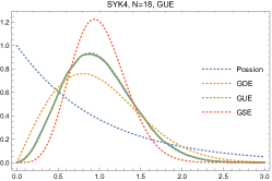
(a) t

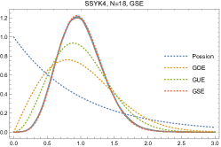
(b) t

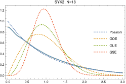
(c) t

(d) t

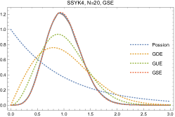
(e) t

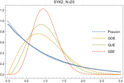
(f) t

(g) t

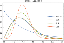
(h) t

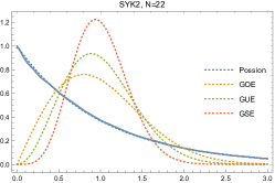
(i) t

(j) t

(k) t

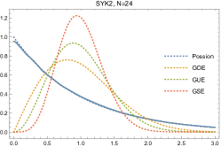
(l) t

Figure 1: Plot of the nearest neighbor energy level spacing distributions of the SYK₄, SSYK₄ and SYK₂ models with $\lambda=0$, $-0.001$, $-0.1$, $-1$, $-10$, $-100$, $-1000$. The curves with different $\lambda$ overlap each other exactly.

3.2 The SFF of the chaotic models

In the following paragraph, we will investigate the SFF of the deformed SYK models. The SFF for a disordered system is [12]:

$$g(t,\beta) =\frac{\left\langle Z(\beta,t)Z^{*}(\beta,t)\right\rangle_{J}}{\langle Z(\beta)\rangle_{J}^{2}}\,,$$ (3.8)

$$g_{d}(t,\beta) =\frac{\langle Z(\beta,t)\rangle_{J}\cdot\left\langle Z^{*}(\beta,t)\right\rangle_{J}}{\langle Z(\beta)\rangle_{J}^{2}}\,,$$

$$g_{c}(t,\beta) =g(t,\beta)-g_{d}(t,\beta)\,,$$

where the disorder average is taken separately in the numerator and denominator. The late-time behavior of this quantity is complicated but can be extracted by taking the long-time average. In this process, the terms with oscillating phases vanish, and only terms with $E_{m}=E_{n}$ survive. The result is

$$\lim_{T\rightarrow\infty}\frac{1}{T}\int_{0}^{T}dt\left|\frac{Z(\beta,t)}{Z(\beta)}\right|^{2}=\frac{1}{Z(\beta)^{2}}\sum_{E}N_{E}^{2}e^{-2\beta E}\,,$$ (3.9)

where $N_{E}$ is the degeneracy of the energy level $E$. The degeneracy of the Majorana SYK₄ model and the SSYK₄ model have been reviewed in Sec. 2. For the $N$ Majorana SYK₄ model, the energy eigenvalues are doubly degenerate for $N$ mod $8=2$, $4$, $6$ and nondegenerate for $N$ mod $8=0$. For the SSYK₄ model, the energy eigenvalues are quadruply degenerate for $N$ mod $8=2$, $4$ and doubly degenerate for $N$ mod $8=0$, $6$. As a result, the late-time behavior of the SFF of these two types of models at infinite temperature can be summarized as follows

$$\lim_{t\rightarrow\infty}\left|\frac{Z(it)}{Z(0)}\right|^{2}=\begin{cases}\frac{1}{L}\quad N\text{ mod }8=0\\ \frac{2}{L}\quad N\text{ mod }8=2,4,6\end{cases} \text{for Majorana SYK${}_{4}$}\,,$$

$$\lim_{t\rightarrow\infty}\left|\frac{Z(it)}{Z(0)}\right|^{2}=\begin{cases}\frac{2}{L}\quad N\text{ mod }8=0,6\\ \frac{4}{L}\quad N\text{ mod }8=2,4\end{cases} \text{for SSYK${}_{4}$}\,,$$ (3.10)

where $L=2^{N/2}$ is the dimension of the Hilbert space. Recall that the $T\bar{T}$ deformation $H\rightarrow f(H-E_{0})$ preserves the classical integrability of the theory, so the late time behavior of the SFF is unchanged under the $T\bar{T}$ deformation.

For the RMT, $g_{d}(t,0)$ and $g_{c}(t,0)$ behavior as

$$g_{d}(t,0)\sim\frac{1}{t^{3/2}}\quad\text{and}\quad g_{\rm c}(t,0)=\begin{cases}t/(2\pi L^{2}),\quad t<2L\\ 1/(\pi L),\quad t\geq 2L\end{cases}\,,$$ (3.11)

where $L$ is the dimension of the matrix model and corresponds to the dimension of the Hilbert space of the SYK model. According to Eq. (3.11), one can get the “dip time” $t_{d}$ and the “plateau time” $t_{p}$ as $t_{d}\sim L^{1/2}\sim e^{S/2}$ and $t_{p}\sim 2L\sim e^{S}$. Explicitly, the SFF of the original SYK model in the conformal limit is [12]

$$g_{d}(t,\beta)=\frac{\beta^{3}}{(\beta^{2}+t^{2})^{3/2}}\exp\left(-\frac{cNt^{2}}{\beta(\beta^{2}+t^{2})}\right)\,,$$

$$g_{\rm ramp}(t,\beta)\sim\begin{cases}\frac{t}{2\pi}\exp\left[-2Ns_{0}-\frac{cN}{\beta}\right],\quad&t<2\pi e^{Ns_{0}}\,,\\ \frac{t}{2\pi}\exp\left[-2Ns_{0}-\frac{cN}{\beta}-\frac{\beta}{cN}\log^{2}\left(\frac{t/(2\pi)}{e^{Ns_{0}}}\right)\right],\quad&e^{Ns_{0}}<t<t_{p}\\ \exp\left[-Ns_{0}-\frac{3cN}{4\beta}\right],\quad&t>t_{p}\end{cases}\,,$$ (3.12)

where $t_{p}=2\pi e^{Ns_{0}+\frac{cN}{2\beta}}=2\pi e^{S(\beta)}$ and $s_{0}$ is the entropy of the ground state. From Eq. (3.12), one can extract the “dip time” as $t_{d}\sim e^{Ns_{0}/2}$. On the contrary, the time scale of $t_{p}$ for the original SYK₂ model is about $t_{p}\sim N$ which is much smaller than $L\sim 2^{N/2}\sim e^{S}$.

3.3 The SFF in the $T\bar{T}$-deformed SYK₄ models

The SFF defined in Eq. (3.8) of the Majorana SYK₄ model was first discussed in [12] and the curves of $g(t,\beta)$ are in agreement with the RMT results. The SFF of the RMT contains a slope region before the dip time $t_{d}$, a ramp region between $t_{d}$ and the plateau time $t_{p}$, and a plateau region at the late time. The ramp region configuration characterizes the system’s quantum chaotic behavior, and the late time behavior demonstrates the discreteness of the spectrum. As discussed in Eq. (3.10), the value of the SFF at the late time is determined completely by the system’s symmetry. The discussion on the similarity between the SYK model and the RMT was extended to the supersymmetric version [61]. In this case, the systems can be further classified according to the matrix type of the supercharge $Q$. The special structures of the Hamiltonian $H$ are modified from Gaussian to Wishart-Laguerre [65, 66] and the RMT ensembles to which they belong are called LOE and LSE. However, the SFFs of these systems belong to the class of GOE, and GSE [61]. As discussed in [67], the density of states $\rho(E)$ of SSYK models satisfy the Marčenko-Pastur distribution [68] in the large $N$ limit. The slope region of SFF is calculated by the Fourier transformation of the square of $\rho(E)$. The result is

$$g_{d}(t,0)=J_{0}^{2}(2t)+J_{1}^{2}(2t)\,$$ (3.13)

which decay slower than the RMT result in Eq. (3.11). So the ramp region is obscured. However, the ramp region is exposed by subtracting off the disconnected contribution from the SFF. So we display the connected SFF (cSSF) for the SSYK case.

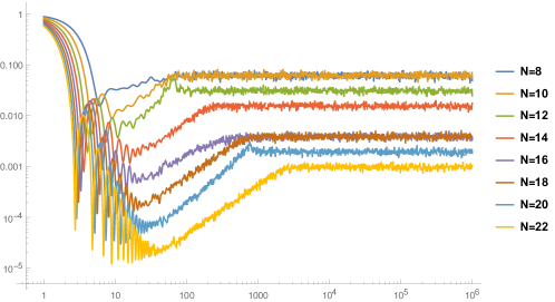
Figure 2: Plot of SFF of the undeformed SYK₄ model with various values of $N$.

In a chaotic model, the late-time behavior of the SFF is controlled by the small level spacing $s$, which approximately obeys the statistic of Gaussian ensembles. Here, we choose GUE statistics for simplicity. The two-point function has the sine kernel [12]

$$R_{2}^{0}(x_{1},x_{2})\approx\left\langle\rho(x)\right\rangle\delta(s)+\left\langle\rho(x_{1})\right\rangle\left\langle\rho(x_{2})\right\rangle\left(1-\frac{\sin^{2}(\pi\left\langle\rho(x)\right\rangle s)}{(\pi\left\langle\rho(x)\right\rangle s)^{2}}\right)\,,$$ (3.14)

where $x=(x_{1}+x_{2})/2$ and $s=x_{1}-x_{2}$. We will take $\rho(x)$ as the one-fold spectral density of the SYK₄ model with $\int\rho(x)dx=2^{N/2-1}$. The SFF of the ${T\bar{T}}$-deformed chaotic theory becomes

$$\left\langle\left|Z_{\lambda}(\beta,t)\right|^{2}\right\rangle= \int_{-\infty}^{\infty}R^{0}_{2}(x_{1},x_{2})e^{-\beta(f_{1}+f_{2})+it(f_{1}-f_{2})}dx_{1}dx_{2}$$

$$\approx \left|\left\langle Z_{\lambda}(\beta,t)\right\rangle\right|^{2}+\int dxe^{-2\beta f(x-E_{0})}\min\left\{\frac{tf^{\prime}(x-E_{0})}{2\pi},\left\langle\rho(x)\right\rangle\right\}\,.$$ (3.15)

Here, we have used (3.4) in the first step and approximated the exponent as $-2\beta f(x-E_{0})+itf^{\prime}(x-E_{0})s$ in the off-diagonal part of the integral in the second step, since the sine kernel is localized around $s=0$. To estimate the integral in the large $N$ limit, we consider the one-fold spectral density of the SYK₄ model near the edge of the spectrum and in the interior respectively as [47, 12, 11, 73]

$$\left\langle\rho(x)\right\rangle=\begin{cases}\sqrt{\frac{2\pi}{cJ_{0}^{3}}}e^{S_{0}}\sinh(\sqrt{2c(\left|E_{0}\right|-\left|x\right|)}),&\left|x\right|\to\left|E_{0}\right|\\ 2^{N/2-1}\frac{1}{\sqrt{2\pi\sigma}}\exp\left(-\frac{x^{2}}{2\sigma}\right),&\left|x\right|\ll\left|E_{0}\right|\end{cases},$$ (3.16)

where $c/2$ is the specific heat, $E_{0}$ is the ground state energy and the variant $\sigma\approx(0.6J_{0})^{2}$ is determined by fitting the numerical spectrum of $N=22$. According to the shape of the spectral density, the cSFF $g_{c}(t)$ with $\beta=0$ has a ramp

$$g_{c}(t)\approx\frac{1-\sqrt{1-16\lambda\left|E_{0}\right|}}{4\lambda}2^{2-N}\frac{t}{2\pi}\sim 2^{2-N}\frac{\left|E_{0}\right|J_{\rm eff}t}{\pi J_{0}}$$ (3.17)

initially and slows down gradually, where $J_{\rm eff}$ is given in (2.27). The ramp surpasses the slope at the dip time $t_{d}\approx 2^{(N-1)/3}\exp\left(-E_{0}{}^{2}/3\sigma\right)\left(\sigma\left|E_{0}\right|\right)^{-1/3}J_{0}/J_{\rm eff}$. The ramp stops at the plateau time $t_{p}\approx\sqrt{2\pi}2^{N/2-1}/(0.6J_{\rm eff})$. So the ramps of different $\lambda$ will overlap with each other as shown in Figure 4c.

In this paragraph, we enumerate the SFFs $g(t,0)$ of the $T\bar{T}$-deformed SYK₄ model in Figure 3a and its supersymmetric extension version in Figure 3b. For comparison, we also repeat the result in [12] and display it in Figure 2. As we can see from the plot in Figure 3a, the $T\bar{T}$-deformed SFF also similarly exhibits the dip, the ramp, and the plateau regions. The value of $t_{d}$ and $t_{p}$ are approximately $O(1)\sim O(10)$ and $O(10)\sim O(10^{3})$, respectively, and agree with the time scale mentioned in the last section. Moreover, the shape of the ramp agrees with the RMT prediction for various $N$. In particular, we can find the kink for $N$ mod $8=4$, which is the feature of the ramp in the GSE ensemble.

The numerical results of the cSFF of the $T\bar{T}$-deformed SSYK₄ model are shown in Figure 3b. By subtracting the disconnected contribution, the figure shows that the pattern of $g(t,0)$ also exhibits the ramp and the plateau region for large enough $N$. The time scale of $t_{d}$ and $t_{p}$ are approximate to the counterpart values of SYK₄. Besides, we find the ramp and plateau connect smoothly in the case of $N$ mod $8=0,\,6$ and connect at a kink in the case of $N$ mod $8=2,\,4$. This property indicates that the SFFs for $N$ mod $8=0,\,6$ follow the GOE behavior, and the SFFs for $N$ mod $8=2,\,4$ follow the GSE behavior. This result agrees with the expectation introduced in Sec. 2.3.

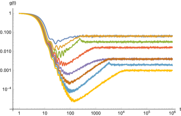
(a) t

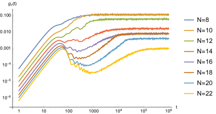
(b) t

Figure 3: Plot of SFF of the (a) deformed SYK₄ model and (b) deformed SSYK₄ model. We choose $\lambda=-1$, $\beta=0$ and a range of $N$ from 8 to 22.

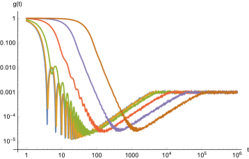
(a) t

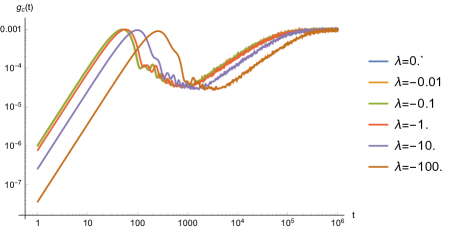
(b) t

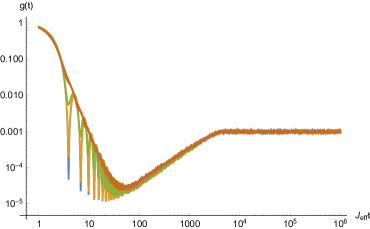
(c) t

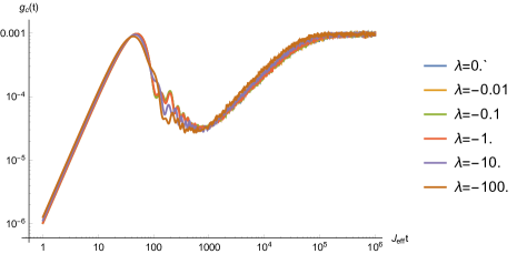
(d) t

Figure 4: (a): SSF of the $T\bar{T}$-deformed SYK₄ model and (b): cSSF of the $T\bar{T}$-deformed SSYK₄ model with various value of $\lambda$. (c): SSF of the $T\bar{T}$-deformed SYK₄ model and (d): cSSF of the $T\bar{T}$-deformed Majorana SSYK₄ model with respect to $J_{\rm eff}t$ and various value of $\lambda$. We choose $N=22$, $\beta=0$ and $\lambda=0$, $-0.01$, $-0.1$, $-1$, $-10$, $-100$.

To study the effect of the $T\bar{T}$ deformation on the SFF more explicitly, we show the SFF (cSSF) of the deformed SYK₄ and SSYK₄ models with different $\lambda$ in Figure 4a and 4b. We find that the image of $g(t,0)$ with different $\lambda$ shifts along the horizon axis by approximately the same amount in the log-log coordinate. As mentioned in Sec. 2.1, the $T\bar{T}$ deformation acting on large-$N$ SYK is equivalent to replacing $J_{0}$ with $J_{\rm eff}(\lambda)$. We show the SFF of SYK₄ and cSSF of SSYK₄ with $T\bar{T}$ deformation in the time units $J_{\rm eff}(\lambda)$ in Figure 4c and 4d. We find that the curves of SFF with different $\lambda$ overlap.

3.4 The SFF in the $T\bar{T}$-deformed SYK₂ models

The SYK₂ model is equivalent to a model of free fermions with a random mass matrix [69, 70, 71]. It can be described with a $N\times N$ random matrix which leads to the “mini-ramp” and the “mini-plateau.” The plateau time $t_{p}\sim N$ (about $O(10)$ in Figure 5b) in this model instead of $t_{p}\sim L$ in the Gaussian random ensemble of RMT. We show $g(t)$ of the deformed SYK₂ models with different $N$ and different $\lambda$ in Figure 5a and Figure 5b respectively. As discussed in the SYK₄ model, the major effect of the $T\bar{T}$ deformation on the SFF is to shift the curves along the horizontal axis parallelly. Moreover, the patterns of SFF with different $\lambda$ overlap with each other in the time unit $J_{\rm eff}$, as shown in Figure 5c.

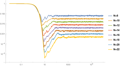
(a) t

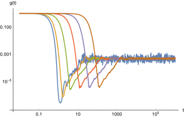
(b) t

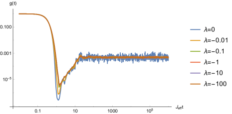
(c) t

Figure 5: (a): SSF of the $T\bar{T}$-deformed SYK₂ with various value of $N$ and $\lambda=-1$. (b): SSF of the $T\bar{T}$-deformed SYK₂ with various value of $\lambda$. (c): SSF of the $T\bar{T}$-deformed SYK₂ with respect to $J_{\rm eff}t$. We choose $N=22$ in (c) and (d).

As reviewed in Sec. 1, we distinguish quantum chaos from other concepts (scrambling and operator growth) and detect quantum chaos signals by SFF. From the results presented in Figure 4c and 5c, we can conclude that the overall effect of the $T\bar{T}$ deformation can be interpreted as a rescaling of the time parameter and the quantum chaotic behavior remains unchanged under the $T\bar{T}$ deformation.

4 The OTOC in the $T\bar{T}$-deformed SYK models

In the previous section, we provided strong evidence with the SFF in the $T\bar{T}$-deformed SYK model that the $T\bar{T}$ deformation does not change the late-time behavior of quantum chaos (or non-chaos) in the original theories. Motivated by recent advances in holography, scrambling became a new quantity to detect the feature of the time evolution of a system at the early time. In this section, we test the early-time behavior and study the effect of the $T\bar{T}$ deformation on the scrambling in deformed theories in more detail by computing the OTOC.

4.1 Analytical results

The out-of-time-ordered correlator is defined by

$$F(t)=-\frac{Z(\beta)\mathrm{Tr}\left(yV(t)yW(0)yV(t)yW(0)\right)}{\mathrm{Tr}(y^{2}Vy^{2}V)\mathrm{Tr}(y^{2}Wy^{2}W)}\,,$$ (4.1)

where $Z(\beta)=\mathrm{Tr}e^{-\beta(H-E_{0})}$ and $y=e^{-\beta(H-E_{0})/4}$. In this work, we calculate the OTOC of Majorana fermions $\psi_{i}$ and $\psi_{j}$ and then average over the index $i$, $j$.

The effect of the ${T\bar{T}}$ deformation on OTOCs of the SYK₄ model is characterized by the effective coupling $J_{\text{eff}}$. When $\beta=0$, the OTOC of SYK model has been investigated in the large-$q$ limit in [72]. The result is

$$F_{\rm OTOC}=1-\frac{1}{2N}\cosh 2\mathcal{J}t\,.$$ (4.2)

It is reasonable to guess that the ${T\bar{T}}$-deformed results are changed by replacing $\mathcal{J}$ to $\mathcal{J}_{\rm eff}$. So the pattern of $F_{\rm OTOC}$ is universal as a function of $J_{\rm eff}t$.

In the conformal limit, the $T\bar{T}$-deformed OTOC and Lyapunov exponent have been discussed in [4, 5]. In conformal limit, the Lyapunov exponent is extracted from the pole of the two point function $\langle\epsilon(u)\epsilon(0)\rangle$ where $\epsilon(u)$ is the fluctuation of the time reparameterization. Under the $T\bar{T}$ deformation, the $SL(2,\mathbb{R})$ symmetries remain unchanged. As a result, the poles contributed to $\langle\epsilon(u)\epsilon(0)\rangle$ remain $n=0,\pm 1$. The OTOC is

$$F_{\rm OTOC}\sim\frac{\beta}{C}\sqrt{1+\lambda C\frac{16\pi^{2}}{\beta^{2}}}e^{\frac{2\pi}{\beta}u}\,,$$ (4.3)

and the Lyapunov exponent $\lambda_{L}=2\pi/\beta$ is unchanged.

The OTOC of the ${T\bar{T}}$-deformed SYK₂ model could be solved by integrability. The original SYK₂ model is free. So the operator $\psi_{i}(t)$ does not grow and the OTOC does not decay. A nontrivial ${T\bar{T}}$ deformation introduces the interaction while maintains the integrability. The OTOC could decay to small values. We will solve the OTOC on the basis $\left|\vec{n}\right\rangle$. We first calculate the denominator in Eq. (4.1) as

$$G(\beta/2)\equiv \frac{1}{NZ(\beta)}\sum_{i}^{N}\mathrm{Tr}\left[y^{2}\psi_{i}y^{2}\psi_{i}\right]$$

$$= \frac{2}{NZ(\beta)}{\rm Re}\sum_{\vec{n}}\sum_{a}^{N/2}\left\langle\vec{n}\right|y^{2}\chi_{a}^{\dagger}y^{2}\chi_{a}\left|\vec{n}\right\rangle$$

$$= \frac{4}{NZ(\beta)}\sum_{a}\sum_{\vec{n}}^{n_{a}=1}\exp\left[-\frac{\beta}{2}(f(E_{\vec{n}})+f(E_{\vec{n}\backslash a}))\right]$$

$$\approx \frac{2}{NZ(\beta)}\sum_{n}\sum_{a}\exp\left[-\beta f(E_{\vec{n}})\right]=1\,,$$ (4.4)

where $E_{\vec{n}\backslash a}=\sum_{b\neq a}n_{b}\varepsilon_{b}$. In the final two steps, we consider large $N$. So we assume $\varepsilon_{a}\ll E_{\vec{n}}$ and $f(E_{\vec{n}})+f(E_{\vec{n}\backslash a})\approx 2f(E_{\vec{n}})$. We further drop the constraint $n_{a}=1$ in the summation of states and compensate for the overcounting by dividing it by $2$. Then the OTOC is

$$F(t)\equiv \frac{-1}{N^{2}Z(\beta)G(\beta/2)^{2}}\sum_{ij}^{N}\mathrm{Tr}\left[y\psi_{i}(t)y\psi_{j}y\psi_{i}(t)y\psi_{j}\right]$$

$$= -\frac{4}{N^{2}Z(\beta)G(\beta/2)^{2}}{\rm Re}\sum_{\vec{n}}\sum_{ab}^{N/2}\left\langle\vec{n}\right|y\chi_{a}^{\dagger}(t)y\chi_{b}^{\dagger}y\chi_{a}(t)y\chi_{b}\left|\vec{n}\right\rangle$$

$$= \frac{16}{N^{2}Z(\beta)G(\beta/2)^{2}}\sum_{a\neq b}\sum_{\vec{n}}^{n_{a}=n_{b}=1}\cos\left[t(f(E_{\vec{n}})-f(E_{\vec{n}\backslash a})-f(E_{\vec{n}\backslash b})+f(E_{\vec{n}\backslash\{a,b\}}))\right]$$

$$\hskip 85.35826pt\times\exp\left[-\frac{\beta}{4}\left(f(E_{\vec{n}})+f(E_{\vec{n}\backslash a})+f(E_{\vec{n}\backslash b})+f(E_{\vec{n}\backslash\{a,b\}})\right)\right]$$

$$\approx \frac{4}{N^{2}Z(\beta)}\sum_{\vec{n}}\sum_{a\neq b}\cos\left(t\varepsilon_{a}\varepsilon_{b}f^{\prime\prime}(E_{\vec{n}})\right)e^{-\beta f(E_{\vec{n}})}$$

$$\approx \frac{2^{2+N/2}}{N^{2}Z(\beta)}\int dEp(E+E_{0})e^{-\beta f(E)}\sum_{a\neq b}\cos\left(t\varepsilon_{a}\varepsilon_{b}f^{\prime\prime}(E)\right)\,.$$ (4.5)

Similarly, in the penultimate step, we assume $\varepsilon_{a,b}\ll E_{\vec{n}}$, approximate the sum and the difference of $f(E)$ functions, drop the constraint $n_{a}=n_{b}=1$ in the summation of states, and compensate the overcounting by dividing it by $4$. In the last step, we introduce the density of states $p(E)$ of the original SYK₂ model. We will work at the large $N$ limit to obtain analytical expressions. Then the single-particle spectrum $\left\{J_{k}\right\}_{k=1}^{N}$ obeys the semi-circle law

$$\rho_{\text{sc}}(\varepsilon)=\frac{1}{2\pi J_{0}}\sqrt{1-\left(\frac{\varepsilon}{4J_{0}}\right)^{2}}$$ (4.6)

and $E_{0}=-4J_{0}N/3\pi$. The density of states $p(E)$ is the Gaussian distribution [11, 73], namely

$$p(E)=\frac{1}{J_{0}\sqrt{\pi N}}\exp\left[-\left(\frac{E}{J_{0}\sqrt{N}}\right)^{2}\right].$$ (4.7)

In principle, one can calculate the OTOC by integrating over $\varepsilon_{a,b}$ and $E$ in (4.5) with the above distributions.

To get an analytical expression, we will consider a saddle point approximation for $E$ at high-temperature limit $\beta J_{0}\ll 1$. According to the distribution $p(E+E_{0})e^{-\beta f(E)}$, $E$ concentrates near the saddle point $E_{c}$ determined by

$$-2\frac{E_{c}+E_{0}}{J_{0}^{2}N}-\beta f^{\prime}(E_{c})=0.$$ (4.8)

We get $E_{c}\sim J_{0}N$. In (4.5), we have $t\varepsilon_{a}\varepsilon_{b}|f^{\prime\prime}(E_{c})|\leq tJ_{0}^{2}/(3\sqrt{3}E_{c})\sim tJ_{0}/N$, which is very small at the early time $t\ll N/J_{0}$. So the cosine function in (4.5) is a flat function of $E$ near $E_{c}$. We take the saddle point value $E_{c}$ in the cosine function and simplify the OTOC as

$$F(t)\approx\frac{4}{N^{2}}\sum_{a\neq b}\cos\left(t\varepsilon_{a}\varepsilon_{b}f^{\prime\prime}(E_{c})\right)=\tilde{F}\left(8J_{0}^{2}f^{\prime\prime}(E_{c})t\right)+O\left(N^{-2}\right),$$ (4.9)

where

$$\tilde{F}(x)= 2\left[\tilde{J}_{0}(x){}^{2}-\frac{\tilde{J}_{1}(x)\tilde{J}_{0}(x)}{x}+\tilde{J}_{1}(x){}^{2}-\frac{1}{N}\left(\tilde{J}_{0}(x)\cos x+\tilde{J}_{1}(x)\sin x\right)\right]$$

$$= 1-\frac{2}{N}-\left(\frac{1}{8}-\frac{1}{2N}\right)x^{2}+O(x^{4})$$ (4.10)

with $\tilde{J}_{i}(x)$ the Bessel function of the first kind. As expected from the expansion of the Hamiltonian (2.19), the OTOCs of the ${T\bar{T}}$-deformed SYK₂ exhibit power law behaviors, which agree with the phenomenon in MBL [28, 29].

4.2 Numerical results

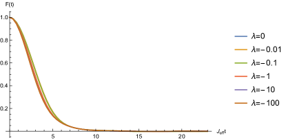
(a) t

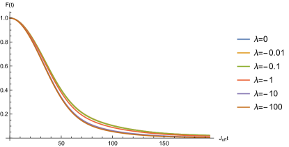
(b) t

Figure 6: Plot of OTOC of (a) SYK₄ model and (b) SSYK₄ model with various value of $\lambda$ at infinite temperature.

In this subsection, we calculate the OTOC numerically. The results of SYK₄ and SYK₂ with different deformation parameter $\lambda$ are shown in Figure 6, 7 and 8. In Figure 6, we can see the exponential decay behavior of OTOC in both the undeformed SYK₄ (SSYK₄) model and the $T\bar{T}$-deformed SYK₄ (SSYK₄) model. The effects of deformation slightly decrease the decay rate. As discussed in the last section, this result can be explained by a rescaling of the coupling constant $J_{0}$. We also plot the OTOC with respect to $J_{\rm eff}t$ and find that the curves with different $\lambda$ coincide precisely, as shown in Figure 6.

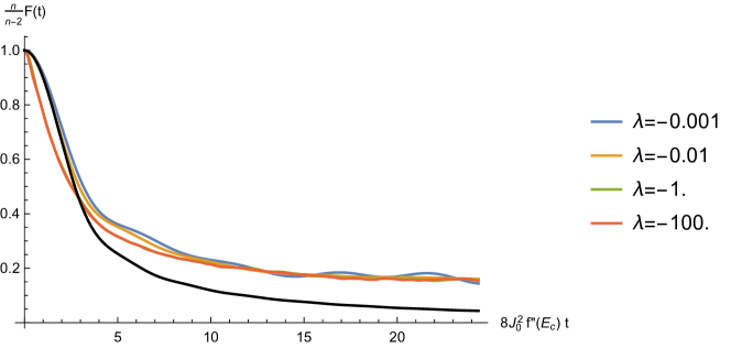
Figure 7: The plot of SYK₂ OTOC with various values of $\lambda$. We choose $N=16$ and the inverse temperature $\beta=0$. The black solid line represents the analytical result calculated by Eq. (4.9). The horizontal axis is $8J_{0}^{2}f^{\prime\prime}(E_{c})t$.

We numerically calculate the OTOCs of the SYK₂ model with or without $T\bar{T}$ deformation and show them in Figures 7 and 8. Based on the Eq. (4.9), we choose the horizontal axis as $J_{0}f^{\prime\prime}(E_{c})t$. Figure 7 shows the OTOC of the SYK₂ model at infinite temperature. For small $\lambda$ ($0<|J_{0}\lambda|\leq 0.01$), OTOCs deviate from unity in the early time as a power law. This behavior of OTOC has been observed in MBL systems [28, 29]. For large $\lambda$ ($|J_{0}\lambda|>0.1$), our numerical results match the Eq. (4.5). We find the saddle-point approximation method (4.9) has a small error. However, the patterns of OTOC with large $\lambda$ in Figure 7 are universal in time units $8J_{0}^{2}f^{\prime\prime}(E_{c})$. The OTOCs at finite temperature is shown in Figure 8. For the high-temperature case ($\beta J_{0}\sim\pi/10$), the features are similar to the one at infinite temperature. One can observe a MBL behavior for small $\lambda$ ($0<|J_{0}\lambda|\leq 0.01$) in Figure 8a. For the low-temperature case ($\beta J_{0}\geq\beta J_{\rm eff}\sim\pi$), the saddle point approximation method is not applicable so the patterns are not uniform with respect to $8J_{0}^{2}f^{\prime\prime}(E_{c})t$. We plot the OTOCs of SYK₂ with $\beta J_{\rm eff}=\pi$ ($\beta J_{0}>\pi$) as the functions of $J_{\rm eff}t$ in Figure 8b.

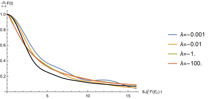
(a) t

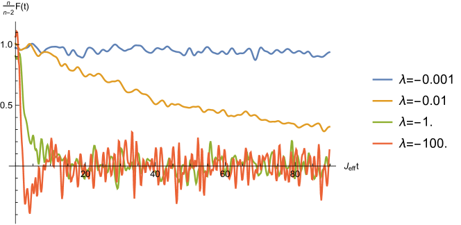
(b) t

Figure 8: OTOC of SYK₂ with (a) $\beta J_{0}=\pi/10$ and with (b) $\beta J_{\rm eff}=\pi/2$. In Figure (a), the black solid lines represent the analytical results and the horizontial axis is $8J_{0}^{2}f^{\prime\prime}(E_{c})t$. In Figure (b), we plot the OTOC as a function of $J_{\rm eff}t$.

5 The K-complexity in the $T\bar{T}$-deformed SYK models

5.1 Lanczos coefficient and K-complexity

In this subsection, we will first give a brief overview of K-complexity. The K-complexity is analogous to the circuit complexity, capturing the intrinsic dynamics of the evolution operator [33]. Given a Hamiltonian $H$ and a certain simple operator $O$ of a system, the K-complexity of $O$ can be measured in the Krylov basis, which is roughly defined as $[H,[H,\cdots,[H,O]]]$. This definition is motivated by the Taylor expansion of the time evolution of a local operator $O$. The Krylov basis can be generated by the Liouvillian superoperator $\mathcal{L}|O)\equiv|[H,O])$. The exact definition of the Krylov basis is

$$|A_{n})=\mathcal{L}|O_{n-1})-b_{n-1}|O_{n-2})\,,$$

$$b_{n}=(A_{n}|A_{n})^{1/2}\,,$$

$$|O_{n})=b^{-1}_{n}|A_{n})\,,$$ (5.1)

where $|O_{0})\equiv|O)$, $b_{0}=0$ by convention. The inner product of the operator basis are $(A|B)=\mathrm{Tr}[A^{\dagger}B]$ in the vacuum state and $(A|B)=\mathrm{Tr}[yA^{\dagger}yB]$ with $y=e^{-\frac{1}{2}\beta\hat{H}}$ in the thermal ensemble. Note that we have regulated the thermal expectation value by splitting the operator of the thermal density matrix. The sequence of positive numbers $\{b_{n}\}$ is called Lanczos coefficients. The number of Krylov basis corresponds to the dimension of the space spanned by the linear operator acting on a Hilbert space. Consider a system described by a $L$-dimensional Hilbert space. The dimension of the operator space is $L^{2}$. For the SYK₄ model, the Heisenberg evolution of a single Majorana fermion $\psi_{i}$ is bounded in the subspace of operators consisting of an odd number of fermions. For the SYK₂ model, the Heisenberg evolution of $\psi_{i}$ is bounded in the subspace of a single particle. Thus, the number of Krylov basis of the SYK₄ and SYK₂ models can be estimated by $d_{\rm Krylov}=(2^{[N/2]})^{2}/2=2^{N-1}$ and $d_{\rm Krylov}=N$, respectively.

More precise calculations of $d_{\rm Krylov}$ have been discussed in [34]. By (5.1), the Krylov basis is the linear span of the action of the Liouvillian superoperator on $O$, namely

$$\left(O,\mathcal{L}O,\mathcal{L}^{2}O,\cdots,\mathcal{L}^{n}O,\cdots\right)^{T}\,.$$ (5.2)

The dimension of this space is the number of the linearly independent vector $\mathcal{L}^{n}O$. We can expand $\mathcal{L}^{n}O$ in the energy basis

$$\mathcal{L}^{n}|O)=\delta_{n0}\sum_{a=1}^{D}O_{aa}|\omega_{aa})+\sum_{a,b=1,a\neq b}^{D}O_{ab}\omega_{ab}^{n}|\omega_{ab})\,,$$ (5.3)

where $|\omega_{ab})=|E_{a}\rangle\langle E_{b}|$ and $\omega_{ab}=E_{a}-E_{b}$ is the eigenvalues of the Liouvillian acting on $|\omega_{ab})$. The matrix representation of (5.3) in this basis is

$$\begin{pmatrix}O_{11}&O_{22}&\cdots&O_{DD}&O_{12}&O_{13}&\cdots&O_{D-1,D}\\ 0&0&\cdots&0&\omega_{12}O_{12}&\omega_{13}O_{13}&\cdots&\omega_{D-1,D}O_{D-1,D}\\ 0&0&\cdots&0&\omega_{12}^{2}O_{12}&\omega_{13}^{2}O_{13}&\cdots&\omega_{D-1,D}^{2}O_{D-1,D}\\ \vdots&\vdots&\ddots&\vdots&\vdots&\vdots&\ddots&\vdots\\ 0&0&\cdots&0&\omega_{12}^{D^{2}-1}O_{12}&\omega_{13}^{D^{2}-1}O_{13}&\cdots&\omega_{D-1,D}^{D^{2}-1}O_{D-1,D}\end{pmatrix}\,.$$ (5.4)

The number of linearly independent vectors in Eq. (5.2) is equal to the rank of the matrix (5.4). The rank of the matrix (5.4) can be calculated as follows. First, we omit the columns containing the zero elements of the matrix $O$, and then we omit the columns containing the repeated eigenvalues $\omega_{ab}$ of $\mathcal{L}$. For the SYK₄ model with $N\text{ mod }8=2,4,6$, the energy level is doubly degenerate. As a result, $\omega_{ab}$ are quadruply degenerate. Similarly, for the SSYK₄ model with $N\text{ mod }8=0,6$, the degeneracy of $\omega_{ab}$ is 4 and for the SSYK₄ model with $N\text{ mod }8=2,4$, the degeneracy of $\omega_{ab}$ is 16. Recall that the transformation $H\rightarrow f(H-E_{0})$ does not break any symmetries of the original theory. Consequently, the degeneracy of $\omega_{ab}$ and $d_{\rm Krylov}$ remain unchanged under the $T\bar{T}$ deformation. For the SYK₂ model, the energy level is non-degenerate but $E_{a}$ comes in pairs with its opposite value $-E_{a}$ for any $a$. In this case, $\omega_{ab}$ is doubly degenerate. For example, for any $E_{a}=-E_{a^{\prime}}$ and $E_{b}=-E_{b^{\prime}}$, we have $\omega_{ab}=E_{a}-E_{b}=E_{b^{\prime}}-E_{a^{\prime}}=\omega_{b^{\prime}a^{\prime}}$. However, the double degeneracy of $\omega_{ab}$ is broken under the $T\bar{T}$ deformation, namely

$$\omega_{ab}^{\lambda}=f(E_{a}-E_{0})-f(E_{b}-E_{0})=f(-E_{a^{\prime}}-E_{0})-f(-E_{b^{\prime}}-E_{0})\neq\omega_{b^{\prime}a^{\prime}}^{\lambda}\,.$$ (5.5)

Under the $T\bar{T}$ deformation, the Krylov space enlarges significantly. We list the $d_{\rm Krylov}$ of the SYK₄, SSYK₄, SYK₂ and the $T\bar{T}$-deformed SYK₂ model with different $N$ in Table 1.

Table 1: Dimension of the operator space

$N$	4	6	8	10	12	14	16	18	20
SYK4	2	12	128	241	512	4032	32768	65281	131072
SSYK4	1	12	57	57	241	4032	16257	16257	65295
SYK2	4	6	8	10	12	14	16	18	20
$T\bar{T}$-deformed SYK2	8	24	64	160	384	896	2048	4608	10240

The Heisenberg evolution $O(t)$ of $O$ can be rewritten as

$$|O(t))=e^{i\mathcal{L}t}|O_{0})\,,$$ (5.6)

and can be expanded on the Krylov basis

$$|O(t))=\sum_{n}i^{n}\varphi_{n}(t)|O_{n})\,.$$ (5.7)

The K-complexity of the Heisenberg operator $O(t)$ is defined as the average of the linear operator $\hat{n}$ in the state $|O(t))$

$$C_{K}(O)=(O(t)|\hat{n}|O(t))=\sum_{n}n|\varphi_{n}(t)|^{2}\,.$$ (5.8)

It is obvious that the magnitude of K-complexity is bounded by the number of Krylov basis. Accordingly, the growth of K-complexity is quantitatively captured by the Lanczos coefficients $\{b_{n}\}$. The asymptotic behavior of the Lanczos coefficients in the large-N limit is $b_{n}\simeq\alpha n^{\delta}$ with $0\leq\delta\leq 1$. By analogy with the behavior of OTOC, it is generally assumed that for the chaotic system, the growth of $b_{n}$ depends linearly on $n$. In this case, the K-complexity is $C_{K}(t)\sim e^{2\alpha t}$ which implies that the Lyapunov exponent is $\lambda_{L}=2\alpha$. However, based on the discussion in Sec. 1 and Sec. 4, we regard $b_{n}$ or $C_{K}$ as another characteristic quantity independent of quantum chaos.

The Lanczos coefficients can be read off from the Hankel determinant $\det(\mu_{2n})$ of the Liouvillian superoperator

$$b_{1}^{2n}\,b_{2}^{2n-2}\cdots b_{n}^{2}=\det(\mu_{i+j})_{0\leq i,j\leq n}\,,$$ (5.9)

where

$$\mu_{2n}\equiv(O_{0}|\mathcal{L}^{2n}|O_{0})$$ (5.10)

is the moments of the Liouvillian superoperator $\mathcal{L}$. From Eq. (5.9), one can show that, for a finite-$N$ system, the asymptotic behavior of the Lanczos coefficients is bounded by [36]

$$b_{n}\leq\begin{cases}\frac{\lambda_{L}}{2}n,\quad 1\ll n\ll N/q\\ \frac{\lambda_{C}}{2}N,\quad N/q\ll n\ll 2^{N}\end{cases}\,,$$ (5.11)

where $\lambda_{L}$ is the Lyapunov exponent and $\lambda_{C}$ is a constant independent of $n$. One can estimate $\lambda_{C}$ by the moments. There is a close relationship between the Green function and the moments

$$G(t)=\frac{Tr[O^{\dagger}(0)O(t)]}{Tr[O^{\dagger}O]}=(O_{0}|e^{i\mathcal{L}t}|O_{0})=\sum_{n}\frac{(it)^{2n}}{(2n)!}(O_{0}|\mathcal{L}^{2n}|O_{0})=\sum_{n}\frac{(it)^{2n}}{(2n)!}\mu_{2n}\,.$$ (5.12)

From Eq. (5.12), we find that the momentum $\mu_{2n}$ is determined completely by the 2-point function $G(t)$. Recall that the conformal 2-point function $G_{c}(t)$ is unchanged under the $T\bar{T}$ deformation. As a result, the Lanczos coefficients, the K-complexity in the conformal limit, and their holographic dual are unchanged under the $T\bar{T}$ deformation.

For a finite $N$ system, it is convenient to express momentum in terms of the energy eigenbasis $|E_{a}\rangle$. According to the ETH conjecture , the matrix elements $O_{ab}$ in the energy basis can be approximated by $O_{ab}=A(E_{a},E_{b})\delta_{ab}+A(E_{a},E_{b})2^{-N/4}R_{ab}$, where $A(E_{a},E_{b})=A(0,0)F(E_{a}-E_{b})$ for $A(0,0)$ a constant and $F$ some function. $R_{ab}$ is a random matrix with zero mean and the variance can be set to 1 by a rescaling. Substituting this expression into the definition (5.10), we obtain

$$\mu_{2n}=2^{-N}\sum_{a,b}(E_{a}-E_{b})^{2n}|F(E_{a}-E_{b})|^{2}\,.$$ (5.13)

From Eq. (5.9) and Eq. (5.13), it is clear that the Lanczos coefficient $b_{n}$ is a constant and is dominated by the largest energy difference with $n\gg N/q$ [36]. It is worth mentioning that the constant Lanczos coefficients $b_{n}$ at large-$n$ capture the linear growth of the K-complexity.

5.2 Numerical results

In this subsection, we present our numerical results on the Lanczos coefficients and the K-complexity of the SYK and SSYK models. We choose the initial simple operator as $O=\psi_{1}$. The Lanczos coefficients of the deformed SYK₄ and SSYK₄ models are shown in Figure 10. The Lanczos coefficients $b_{n}$ in these figures have the same characteristics: a linearly increasing part and a constant part. Before explaining this result in more detail, we first try to analyze the parameters dependence of $b_{n}$. In general, $b_{n}$ should be a function of the inverse temperature $\beta$ and the coupling constant $J$, namely $b_{n}=b_{n}(\beta,J)$. In this paragraph, we omit the subscript of $J$ and label both $J_{0}$ and $J_{\rm eff}$ by $J$. According to Eq. (5.11), the growth rate in the linearly increasing part of $b_{n}$ is expected to be half of the Lyapunov exponent $\lambda_{L}$. The Lyapunov exponent of the SYK₄ model can be estimated in the large-$q$ limit [47] by

$$\lambda_{L}=\frac{2\pi}{\beta}v,\quad\text{where}\quad\beta\mathcal{J}=\frac{\pi v}{\cos(\frac{\pi v}{2})}\quad\text{and}\quad\mathcal{J}=\frac{J}{\sqrt{2}}\,.$$ (5.14)

From Eq. (5.14), we can deduce that $\lambda_{L}/J$ depends on $\beta J$ alone, and $b_{n}/J$ is a function of the single variable $\beta J$ in the linearly increasing part. Moreover, the asymptotic value of $b_{n}$ at large $n$ is dominated by the largest energy difference. We show the deformed largest energy difference as a function of $\lambda$ in Figure 9. Of course, the largest energy difference is proportional to the coupling constant $J$. Thus, the value of $b_{n}/J$ in this part should be universal. Combined with the previous discussion, we can expect that the dimensionless quantity $b_{n}/J$ depends only on $\beta J$ and is universal for large $n$. Under the ${T\bar{T}}$ deformation, the largest energy different is $f(E_{\rm max}-E_{0})$. In order to match the asymptotic value of $b_{n}$, we redefine the effective coupling $J_{\rm eff}$ in this section by

$$J_{\rm eff}=J_{0}\frac{f(E_{\rm max}-E_{0})}{E_{\rm max}-E_{0}}\,.$$ (5.15)

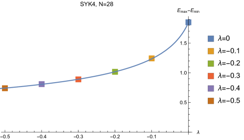
Figure 9: Plot of the maximum energy difference of the SYK₄ with respect to the deformation coefficient $\lambda$. The solid squares label the asymptotic values of $b_{n}$ with different $\lambda$.

In Sec. 3.2 and 4, we explain the effect of the $T\bar{T}$ deformation as the rescaling of the coupling constant $J_{0}$ and find that the SFF and OTOC with different $\lambda$ coincide with each other in the time units $J_{\rm eff}(\lambda)$. So it is rational to expect that the effect of $T\bar{T}$ deformation on $b_{n}$ is also equivalent to the rescaling of the original coupling $J_{0}$, namely

$$b_{n}^{\lambda}(\beta,J_{0})=b_{n}^{0}(\beta,J_{\rm eff})\,.$$ (5.16)

Note that the right-hand side of Eq. (5.16) is equal to $J_{\rm eff}(\lambda)b_{n}^{0}(\beta J_{\rm eff}(\lambda))$ according to the previous analysis. Thus, the dimensionless quantity $b_{n}^{\lambda}/J_{\rm eff}$ is only a function of $\beta J_{\rm eff}(\lambda)$ and is universal at large $n$. $J_{\rm eff}(\lambda)$ is determined by $\lambda$ and Eq. (5.15). We also denote $\lambda$ by a dimensionless parameter $J_{\rm eff}(\lambda)/J_{0}$. Note that $J_{\rm eff}/J_{0}=1$ means that $\lambda=0$ and we recover the undeformed theory in this case.

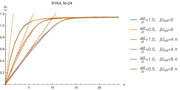
(a) t

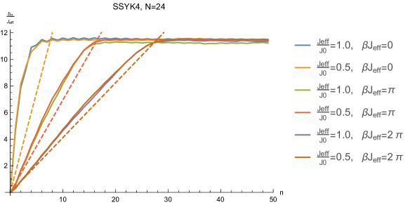
(b) t

Figure 10: In Figure (a) and (b), we display the Lanczos coefficients $b_{n}^{\lambda}$ of the SYK₄ and SSYK₄ in the unit $J_{\rm eff}(\lambda)$ with various values of $\lambda$. $b_{n}^{\lambda}$ depends on dimensionless parameters $J_{\rm eff}(\lambda)/J_{0}$ and $\beta J_{\rm eff}$. Dashed lines represent the Lyapunov exponents over $2J_{\rm eff}$ calculated in the large-$q$ limit.

Based on the previous analysis, we plotted $b_{n}^{\lambda}/J_{\rm eff}(\lambda)$ of the SYK₄ and SSYK₄ models against different dimensionless parameters $\beta J_{\rm eff}(\lambda)$ and $J_{\rm eff}(\lambda)/J_{0}$. One can easily notice that the results presented in Figure 10 are consistent with our analysis. The patterns with the same $\beta J_{\rm eff}$ but different $J_{\rm eff}/J_{0}$ coincide very well, and the asymptotic values at large $n$ are universal. For comparison, we also compute $\lambda_{L}/2J_{\rm eff}$ of SYK₄ and SSYK₄ in the large $q$ limit and represent them by the dashed lines in Figure 10.

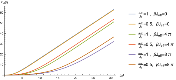
(a) t

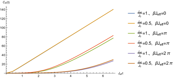
(b) t

Figure 11: K-complexity for (a) SYK₄ and (b) SSYK₄ model with various values of $\beta J_{\rm eff}$ and $J_{\rm eff}/J_{0}$.

In Figure 11, we show the K-complexity of the deformed SYK₄ and SSYK₄ models. In these two figures, the K-complexity shares the same behavior: exponential and linear growth in the initial time. The exponential growth of K-complexity is not obvious due to the small system size. Similar to Figure. 10, we show the results with different dimensionless parameters $\beta J_{\rm Jeff}$ and $J_{\rm eff}/J_{0}$. For the Lanczos coefficients, we have shown that $b_{n}^{\lambda}/J_{\rm eff}$ is universal for fixed $\beta J_{\rm eff}$. This result is equivalent to saying that $C_{K}(t)$ is universal as a function of $J_{\rm eff}t$ for fixed $\beta J_{\rm eff}$. From Figure 11, it is clear that the patterns coincide with the same $\beta J_{\rm eff}$. The small error is due to the small number of ensembles we took. The behavior for different $\beta J_{\rm eff}$ in the early time reflects that the Lyapunov exponents depend on $\beta J_{\rm eff}$ alone. The linear growth rate is universal because the asymptotic values of $b^{\lambda}_{n}/J_{\rm eff}$ are universal for arbitrary parameters.

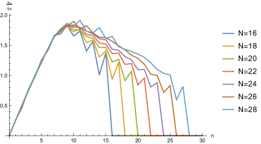
(a) t

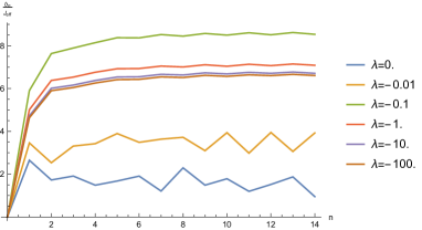
(b) t

Figure 12: (a): $b_{n}$ for the initial SYK₂ with different $N$. (b): $b_{n}$ for the SYK₂ with different $\lambda$ at infinite temperature.

In Sec. 3.4 and 4.2, the SFF and OTOC results show that the original SYK₂ model is a free theory and the $T\bar{T}$-deformed SYK₂ model is a theory of interaction by integrability. In this paragraph, we study this property in more detail by using the Lanczos coefficient. The Lanczos coefficients $b_{n}$ with different $N$ and $\lambda$ are shown in Figure 12 and 13, respectively. Note that the original SYK₂ model is a free theory and the dimension of the Krylov basis is $N$, so the number of nonzeros $b_{n}$ is $N-1$. This property is demonstrated in Figure 12a.

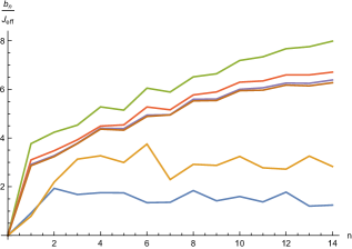
(a) t

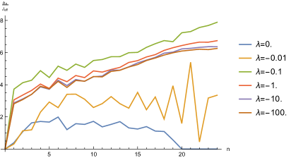
(b) t

Figure 13: Dimensionless Lanczos coefficients $b_{n}^{\lambda}/J_{\rm eff}$ of the SYK₂ model with various values of $\lambda$, where $N=20$, (a) $\beta J_{\rm eff}=\pi$ and (b) $\beta J_{\rm eff}=2\pi$.

In Figure 7 and 8b we observe a MBL like behavior of OTOC for small $\lambda$ ($0<|J_{0}\lambda|\leq 0.01$ in Figure 7) case. However, the deviation from the unity of the OTOCs is always slower than the exponential function for all the $\lambda$. For K-complexity, the chaotic signal is expected to be detected by the early behavior of $b_{n}$ at infinite temperature [33]. The results are plotted in Figure 12b. We find that $b_{n}/J_{\rm eff}$ for vanishing or small $\lambda$ are non-growth. For large $\lambda$, $b_{n}/J_{\rm eff}$ grow initially but are slower than the linear function and then reach the asymptotic values. It is also interesting to study the effect of $T\bar{T}$ deformation on $b_{n}$ at finite temperature. We list our results in Figure 13. For large $\lambda$, we find a significant linear growth regions for large $\beta J_{\rm eff}$ in Figure 13a ($1\leq n\lesssim 11$) and 13b ($1\leq n\lesssim 20$) and we can estimate that the growth rate of $b_{n}/J_{\rm eff}$ is about $1/\beta J_{\rm eff}$. It’s worth noting that the linear growth region still exists even though the deformation vanishes. This feature is exhibited in Figure 12a more clearly. However, these undeformed results are harmless because the dimension of the operator space is small and $C_{K}(t)$ oscillates with time rapidly. But for the deformed case, the operator space is extended shown in Table 1. In this case, $C_{K}(t)$ grows exponentially and then linearly which is similar to the results of the SYK₄ model. As a result, we suggest that the K-complexity is not a suitable quantity to detect quantum chaos at finite temperatures.

6 Summary and prospect

We have investigated the quantum chaotic behaviors of the SYK models with the $T\bar{T}$ deformation. For comparison, we considered the (S)SYK₄ model and the SYK₂ model. The first two models are chaotic and the last model is integrable. In the literature, there is no mathematical definition of quantum chaos. However, it is commonly believed that the energy level spacing captures the main feature of quantum chaos. In this work, we detected the signals of quantum chaos through the SFF. Up to the time rescaling, we found that the $T\bar{T}$ deformation does not affect the properties of quantum chaos. Based on this assertion, we further investigate the effects of the $T\bar{T}$ deformation on scrambling and operator growth captured by OTOC and K-complexity, respectively. We summarize our main results in Table 2.

Table 2: Summary of the results at infinite temperature

		SFF	OTOC	Lanczos
(S)SYK4	All $\lambda$	chaotic	$F(t)\sim 2-e^{\lambda_{L}t}$	$b_{n}\sim\mathcal{J}n$
SYK2	$\lambda=0$	non-chaotic	$F(t)\sim 1$	non-growth
	$|\lambda|\ll 1$	non-chaotic	$F(t)\sim 1-\alpha t^{2}$	non-growth
	$|\lambda|\gg 1$	non-chaotic	$F(t)\sim 1-\alpha t^{2}$	$b_{n}=an^{\delta}$, $\delta<1$

• For the (S)SYK₄ model, the effect of $T\bar{T}$ deformation on SFF, OTOC, and K-complexity is equivalent to a rescaling of the coupling constant $J_{0}$. The patterns of these quantities as functions of $J_{\rm eff}t$ do not depend on $J_{\rm eff}/J_{0}$, but only on $\beta J_{\rm eff}$. At the late time, the OTOC decays to near zero. So the scrambling remains unchanged. The K-complexity in the ${T\bar{T}}$-deformed SYK4 also exhibits an exponential-to-linear growth at an early time. The Lanczos coefficient increases linearly and then saturates, whose slope matches the Lyapunov exponent in the ${T\bar{T}}$-deformed OTOC consistently.

• For the SYK₂ model, the effect of $T\bar{T}$ deformation on SFF is also equivalent to a rescaling of the coupling constant $J_{0}$. For the scrambling, the deviation from the unity of OTOCs with the ${T\bar{T}}$-deformation is slower than the exponential function. For the small $\lambda$ case, we find an MBL behavior for both the infinite temperature case and the finite temperature case. So the ${T\bar{T}}$-deformation here strongly affects the scrambling compared to the original SYK₂ model, whose OTOC does not decay. Then we investigated the operator growth, namely Lanczos coefficients. At infinite temperature, the initial growth of $b_{n}$ is always slower than the linear function. The behaviors of OTOC and operator growth are in agreement with the expectation of the features of the non-chaotic system. At finite temperature, the Lanczos coefficient exhibits a linear growth region in SYK₂ (non-chaotic system) with or without the $T\bar{T}$ deformation, so we suggest that the K-complexity is not a suitable quantity to detect the quantum chaos in this case.

The systems in MBL phases exhibit many interesting features, such as a logarithmic increase of the entanglement entropy [29] and zero diffusion [75]. The ${T\bar{T}}$-deformed SYK₂ model and its spatial generalizations would be the ideal platforms for studying these phenomena of the MBL. Also, we also expect MBL phases in other integrable models with ${T\bar{T}}$ deformation.

References

- [1] A. B. Zamolodchikov, “Expectation value of composite field T anti-T in two-dimensional quantum field theory,” [arXiv:hep-th/0401146 [hep-th]].
- [2] F. A. Smirnov and A. B. Zamolodchikov, “On space of integrable quantum field theories,” Nucl. Phys. B 915, 363-383 (2017) [arXiv:1608.05499 [hep-th]].
- [3] A. Cavaglià, S. Negro, I. M. Szécsényi and R. Tateo, “-deformed 2D Quantum Field Theories,” JHEP 10, 112 (2016) [arXiv:1608.05534 [hep-th]].
- [4] D. J. Gross, J. Kruthoff, A. Rolph and E. Shaghoulian, “ in AdS2 and Quantum Mechanics,” Phys. Rev. D 101, no.2, 026011 (2020) [arXiv:1907.04873 [hep-th]].
- [5] D. J. Gross, J. Kruthoff, A. Rolph and E. Shaghoulian, “Hamiltonian deformations in quantum mechanics, , and the SYK model,” Phys. Rev. D 102, no.4, 046019 (2020) [arXiv:1912.06132 [hep-th]].
- [6] S. He and Z. Y. Xian, “ deformation on multi-quantum mechanics and regenesis,” [arXiv:2104.03852 [hep-th]].
- [7] S. Chakraborty and A. Mishra, “ and deformations in quantum mechanics,” JHEP 11, 099 (2020) [arXiv:2008.01333 [hep-th]].
- [8] O. Bohigas, M. J. Giannoni and C. Schmit, “Characterization of chaotic quantum spectra and universality of level fluctuation laws,” Phys. Rev. Lett. 52, 1-4 (1984)
- [9] T. Guhr, A. Muller-Groeling and H. A. Weidenmuller, “Random matrix theories in quantum physics: Common concepts,” Phys. Rept. 299, 189-425 (1998) [arXiv:cond-mat/9707301 [cond-mat]].
- [10] P.H.C. Lau, C-T. Ma, J. Murugan and M. Tezuka, Correlated disorder in the SYK2 model, J. Phys. A 54 9 095401 (2021)
- [11] A. M. García-García and J. J. M. Verbaarschot, “Spectral and thermodynamic properties of the Sachdev-Ye-Kitaev model,” Phys. Rev. D 94 (2016) no.12, 126010 [arXiv:1610.03816 [hep-th]].
- [12] J. S. Cotler, G. Gur-Ari, M. Hanada, J. Polchinski, P. Saad, S. H. Shenker, D. Stanford, A. Streicher and M. Tezuka, “Black Holes and Random Matrices,” JHEP 05, 118 (2017) [erratum: JHEP 09, 002 (2018)] [arXiv:1611.04650 [hep-th]].
- [13] P. H. C. Lau, C. T. Ma, J. Murugan and M. Tezuka, “Randomness and Chaos in Qubit Models,” Phys. Lett. B 795, 230-235 (2019) [arXiv:1812.04770 [hep-th]].
- [14] Y. Sekino and L. Susskind, “Fast Scramblers,” JHEP 10, 065 (2008) [arXiv:0808.2096 [hep-th]].
- [15] S. H. Shenker and D. Stanford, “Stringy effects in scrambling,” JHEP 05, 132 (2015) [arXiv:1412.6087 [hep-th]].
- [16] J. Maldacena, S. H. Shenker and D. Stanford, “A bound on chaos,” JHEP 08, 106 (2016) [arXiv:1503.01409 [hep-th]].
- [17] D. A. Roberts and D. Stanford, “Two-dimensional conformal field theory and the butterfly effect,” Phys. Rev. Lett. 115, no.13, 131603 (2015) [arXiv:1412.5123 [hep-th]].
- [18] E. B. Rozenbaum, L. A. Bunimovich and V. Galitski, “Early-Time Exponential Instabilities in Nonchaotic Quantum Systems,” Phys. Rev. Lett. 125, no.1, 014101 (2020) [arXiv:1902.05466 [quant-ph]].
- [19] T. Xu, T. Scaffidi and X. Cao, “Does scrambling equal chaos?,” Phys. Rev. Lett. 124, no.14, 140602 (2020) [arXiv:1912.11063 [cond-mat.stat-mech]].
- [20] K. Hashimoto, K. B. Huh, K. Y. Kim and R. Watanabe, “Exponential growth of out-of-time-order correlator without chaos: inverted harmonic oscillator,” JHEP 11 (2020), 068 [arXiv:2007.04746 [hep-th]].
- [21] S. H. Shenker and D. Stanford, “Black holes and the butterfly effect,” JHEP 03, 067 (2014) [arXiv:1306.0622 [hep-th]].
- [22] D. A. Roberts, D. Stanford and L. Susskind, “Localized shocks,” JHEP 03, 051 (2015) [arXiv:1409.8180 [hep-th]].
- [23] S. H. Shenker and D. Stanford, “Multiple Shocks,” JHEP 12, 046 (2014) [arXiv:1312.3296 [hep-th]].
- [24] Goldstein, Sheldon and Huse, David A. and Lebowitz, Joel L. and Tumulka, Roderich, “Thermal Equilibrium of a Macroscopic Quantum System in a Pure State,” Phys. Rev. Lett. 115 (2015), 100402 [arXiv:1506.07494 [cond-mat.stat-mech]].
- [25] R. Nandkishore and D. A. Huse, “Many body localization and thermalization in quantum statistical mechanics,” Ann. Rev. Condensed Matter Phys. 6 (2015), 15-38 [arXiv:1404.0686 [cond-mat.stat-mech]].
- [26] P. W. Anderson, “Absence of Diffusion in Certain Random Lattices,” Phys. Rev. 109 (1958), 1492-1505
- [27] L. Fleishman and P. W. Anderson, “Interactions and the Anderson transition,” Phys. Rev. B 21 2366
- [28] Y. Huang, Y. Zhang and X. Chen, “Out-of-time-ordered correlators in many-body localized systems,” Annalen Phys. 529 (2017) no.7, 1600318 [arXiv:1608.01091 [cond-mat.dis-nn]].
- [29] R. Fan, P. Zhang, H. Shen and H. Zhai, “Out-of-Time-Order Correlation for Many-Body Localization,” Sci. Bull. 62 (2017), 707-711 [arXiv:1608.01914 [cond-mat.quant-gas]].
- [30] V. Khemani, A. Vishwanath and D. A. Huse, “Operator spreading and the emergence of dissipation in unitary dynamics with conservation laws,” Phys. Rev. X 8, no.3, 031057 (2018) [arXiv:1710.09835 [cond-mat.stat-mech]].
- [31] S. Xu and B. Swingle, “Accessing scrambling using matrix product operators,” Nature Phys. 16, no.2, 199-204 (2019) [arXiv:1802.00801 [quant-ph]].
- [32] S. Xu and B. Swingle, “Locality, Quantum Fluctuations, and Scrambling,” Phys. Rev. X 9, no.3, 031048 (2019) [arXiv:1805.05376 [cond-mat.str-el]].
- [33] D. E. Parker, X. Cao, A. Avdoshkin, T. Scaffidi and E. Altman, “A Universal Operator Growth Hypothesis,” Phys. Rev. X 9, no.4, 041017 (2019) [arXiv:1812.08657 [cond-mat.stat-mech]].
- [34] J. L. F. Barbón, E. Rabinovici, R. Shir and R. Sinha, “On The Evolution Of Operator Complexity Beyond Scrambling,” JHEP 10, 264 (2019) [arXiv:1907.05393 [hep-th]].
- [35] A. Avdoshkin and A. Dymarsky, “Euclidean operator growth and quantum chaos,” Phys. Rev. Res. 2, no.4, 043234 (2020) [arXiv:1911.09672 [cond-mat.stat-mech]].
- [36] S. K. Jian, B. Swingle and Z. Y. Xian, “Complexity growth of operators in the SYK model and in JT gravity,” JHEP 03, 014 (2021) [arXiv:2008.12274 [hep-th]].
- [37] E. Rabinovici, A. Sánchez-Garrido, R. Shir and J. Sonner, “Operator complexity: a journey to the edge of Krylov space,” JHEP 06, 062 (2021) [arXiv:2009.01862 [hep-th]].
- [38] A. Kar, L. Lamprou, M. Rozali and J. Sully, “Random matrix theory for complexity growth and black hole interiors,” JHEP 01, 016 (2022) [arXiv:2106.02046 [hep-th]].
- [39] P. Caputa, J. M. Magan and D. Patramanis, “Geometry of Krylov complexity,” Phys. Rev. Res. 4 (2022) no.1, 013041 [arXiv:2109.03824 [hep-th]].
- [40] N. Hörnedal, N. Carabba, A. S. Matsoukas-Roubeas and A. del Campo, “Ultimate Physical Limits to the Growth of Operator Complexity,” [arXiv:2202.05006 [quant-ph]].
- [41] V. Balasubramanian, P. Caputa, J. M. Magan and Q. Wu, “Quantum chaos and the complexity of spread of states,” Phys. Rev. D 106 (2022) no.4, 046007 [arXiv:2202.06957 [hep-th]].
- [42] V. Balasubramanian, J. M. Magan and Q. Wu, “A Tale of Two Hungarians: Tridiagonalizing Random Matrices,” [arXiv:2208.08452 [hep-th]].
- [43] B. Bhattacharjee, X. Cao, P. Nandy and T. Pathak, JHEP 05 (2022), 174 doi:10.1007/JHEP05(2022)174 [arXiv:2203.03534 [quant-ph]].
- [44] S. Baek, “Krylov complexity in inverted harmonic oscillator,” [arXiv:2210.06815 [quant-ph]].
- [45] S. He and H. Shu, “Correlation functions, entanglement and chaos in the -deformed CFTs,” JHEP 02, 088 (2020) [arXiv:1907.12603 [hep-th]].
- [46] S. He, “Note on higher-point correlation functions of the or deformed CFTs,” Sci. China Phys. Mech. Astron. 64, no.9, 291011 (2021) [arXiv:2012.06202 [hep-th]].
- [47] J. Maldacena and D. Stanford, “Remarks on the Sachdev-Ye-Kitaev model,” Phys. Rev. D 94, no.10, 106002 (2016) [arXiv:1604.07818 [hep-th]].
- [48] S. Dubovsky, V. Gorbenko and G. Hernández-Chifflet, “ partition function from topological gravity,” JHEP 09, 158 (2018) [arXiv:1805.07386 [hep-th]].
- [49] S. Dubovsky, V. Gorbenko and M. Mirbabayi, “Asymptotic fragility, near AdS2 holography and ,” JHEP 09, 136 (2017) [arXiv:1706.06604 [hep-th]].
- [50] J. Cardy, “The deformation of quantum field theory as random geometry,” JHEP 10, 186 (2018) [arXiv:1801.06895 [hep-th]].
- [51] R. Conti, S. Negro and R. Tateo, “The perturbation and its geometric interpretation,” JHEP 02, 085 (2019) [arXiv:1809.09593 [hep-th]].
- [52] J. Aguilera-Damia, V. I. Giraldo-Rivera, E. A. Mazenc, I. Salazar Landea and R. M. Soni, “A path integral realization of joint , and flows,” JHEP 07, no.07, 085 (2020) [arXiv:1910.06675 [hep-th]].
- [53] A. J. Tolley, “ deformations, massive gravity and non-critical strings,” JHEP 06, 050 (2020) [arXiv:1911.06142 [hep-th]].
- [54] E. A. Mazenc, V. Shyam and R. M. Soni, “A Deformation for Curved Spacetimes from 3d Gravity,” [arXiv:1912.09179 [hep-th]].
- [55] A. Kitaev, “Hidden correlations in the Hawking radiation and thermal noise.” Talk at KITP http://online.kitp.ucsb.edu/online/joint98/kitaev/, February, 2015.
- [56] A. Kitaev, “A simple model of quantum holography.” Talks at KITP http://online.kitp.ucsb.edu/online/entangled15/kitaev/ and http://online.kitp.ucsb.edu/online/entangled15/kitaev2/, April and May, 2015.
- [57] W. Fu and S. Sachdev, “Numerical study of fermion and boson models with infinite-range random interactions,” Phys. Rev. B 94, no.3, 035135 (2016) [arXiv:1603.05246 [cond-mat.str-el]].
- [58] Y. Z. You, A. W. W. Ludwig and C. Xu, “Sachdev-Ye-Kitaev Model and Thermalization on the Boundary of Many-Body Localized Fermionic Symmetry Protected Topological States,” Phys. Rev. B 95, no.11, 115150 (2017) [arXiv:1602.06964 [cond-mat.str-el]].
- [59] Serbyn, Maksym and Papić, Z. and Abanin, Dmitry A, “Local Conservation Laws and the Structure of the Many-Body Localized States,” Phys. Rev. Lett. 111, no.12, 127201 (2013) [arXiv:1305.5554 [cond-mat.dis-nn]].
- [60] W. Fu, D. Gaiotto, J. Maldacena and S. Sachdev, “Supersymmetric Sachdev-Ye-Kitaev models,” Phys. Rev. D 95, no.2, 026009 (2017) [arXiv:1610.08917 [hep-th]].
- [61] T. Li, J. Liu, Y. Xin and Y. Zhou, “Supersymmetric SYK model and random matrix theory,” JHEP 06, 111 (2017) [arXiv:1702.01738 [hep-th]].
- [62] D. Stanford and E. Witten, “JT gravity and the ensembles of random matrix theory,” Adv. Theor. Math. Phys. 24, no.6, 1475-1680 (2020) [arXiv:1907.03363 [hep-th]].
- [63] T. Guhr, A. Muller-Groeling and H. A. Weidenmuller, “Random matrix theories in quantum physics: Common concepts,” Phys. Rept. 299, 189-425 (1998) [arXiv:cond-mat/9707301 [cond-mat]].
- [64] M.L. Mehta, “Random Matrices,” volume 142, Academic Press (2004)
- [65] I. Dumitriu and A. Edelman, Journal of Mathematical Physics, 43(11), 5830–5847
- [66] A. Edelman and N. R. Rao, “Random matrix theory,” Acta Numerica14, 233–297
- [67] N. Hunter-Jones and J. Liu, “Chaos and random matrices in supersymmetric SYK,” JHEP 05 (2018), 202 [arXiv:1710.08184 [hep-th]].
- [68] V. A. Marčenko and L. A. Pastur “Distribution of eigenvalues for some sets of random matrices,” Math. USSR-Sb. 1 (1967) 457 [Mat. Sb. 72 (1967) 507]
- [69] D. J. Gross and V. Rosenhaus, “A Generalization of Sachdev-Ye-Kitaev,” JHEP 02, 093 (2017) [arXiv:1610.01569 [hep-th]].
- [70] J. M. Magan, “Random free fermions: An analytical example of eigenstate thermalization,” Phys. Rev. Lett. 116, no.3, 030401 (2016) [arXiv:1508.05339 [quant-ph]].
- [71] D. Anninos, T. Anous and F. Denef, “Disordered Quivers and Cold Horizons,” JHEP 12, 071 (2016) [arXiv:1603.00453 [hep-th]].
- [72] D. A. Roberts, D. Stanford and A. Streicher, “Operator growth in the SYK model,” JHEP 06 (2018), 122 [arXiv:1802.02633 [hep-th]].
- [73] R. Feng, G. Tian and D. Wei, “Spectrum of SYK model,” [arXiv:1801.10073 [math-ph]].
- [74] A. M. García-García and M. Tezuka, “Many-body localization in a finite-range Sachdev-Ye-Kitaev model and holography,” Phys. Rev. B 99 (2019) no.5, 054202 [arXiv:1801.03204 [hep-th]].
- [75] S. K. Jian and H. Yao, “Solvable Sachdev-Ye-Kitaev models in higher dimensions: from diffusion to many-body localization,” Phys. Rev. Lett. 119, no.20, 206602 (2017) [arXiv:1703.02051 [cond-mat.str-el]].