Gradient flow step-scaling function for SU(3) with $N_{f}=6$ or $4$ fundamental flavors

Abstract

Nonperturbative determinations of the renormalization group (RG) $\beta$ function are crucial to understand properties of gauge-fermion systems at strong coupling and connect lattice simulations and the perturbative ultraviolet regime. Choosing well-understood, QCD-like systems with SU(3) gauge group and either six or four fundamental flavors, we investigate their step-scaling $\beta$ function. In both cases we push the simulations to the boundary of chiral symmetry breaking and study the regime $g^{2}_{GF}\lesssim 8.2$ with six, and $g^{2}_{GF}\lesssim 6.6$ with four flavors. We carefully consider the lattice discretization errors by comparing three different gradient flows (GF), and for each flow three operators to estimate the renormalized finite volume coupling. We also consider the tree level improvement of the coupling. Noteworthy outcome is that nonperturbatively determined $\beta$ functions run much slower than perturbatively predicted.

I Introduction

Nonperturbative lattice calculations are essential to account for nonperturbative effects when comparing experimental and theoretical predictions in search of new, beyond standard model (SM) physics effects Kronfeld et al. (2022); Davoudi et al. (2022). An important part of the lattice program is to connect the energy range accessible in the lattice simulation to the UV scale where reliable connection to perturbation theory is possible. The nonperturbative renormalization group (RG) $\beta$ function provides this connection for the renormalized coupling.

Several lattice approaches exist to predict the RG $\beta$ function. Many of the recent calculations use the gradient flow (GF) renormalized coupling $g_{GF}^{2}$ Narayanan and Neuberger (2006); Lüscher (2010, 2010), and predict the finite volume step-scaling function or the infinite volume continuous $\beta$ function Fodor et al. (2012); Lüscher (2014); Hasenfratz and Witzel (2020); Fodor et al. (2018a). In the former the flow time (or energy scale) is set by the lattice size $t=(cL)^{2}/8$ and the step-scaling function $\beta_{c,s}$ is calculated by comparing the GF coupling on lattice sizes $L$ and $sL$ Fodor et al. (2012). The finite volume step-scaling method requires that the lattice size provides the only dimensional scale, i.e. it is not applicable in the confining, chirally broken regime. Thus, when investigating QCD-like systems it is important to keep the lattice volume small so the simulations are performed in the deconfined regime. This condition limits both the bare coupling and the accessible renormalized coupling range. The continuous $\beta(g^{2})$ function is defined analogous to the continuum definition and requires that the lattice data are extrapolated to infinite volume Hasenfratz and Witzel (2020, 2019); Fodor et al. (2018a). This method is applicable even when another energy scale emerges, e.g. in the chirally broken/confining regime.

Both the step-scaling and continuous $\beta$ functions are defined in the chiral limit. While simulations with zero fermion mass are possible in the finite volume deconfined phase, the chirally broken/confining regime is accessible only with finite mass simulations. Consequently the analysis requires to also take the $am_{f}\to 0$ chiral limit. To date only preliminary results predicting the RG $\beta$ function in the confined phase have been reported for the $N_{f}=0$ pure gauge system in Ref. Peterson et al. (2021) and for $N_{f}=2$ in Ref. Hasenfratz et al. (2022).

Both methods predict that QCD-like systems with $N_{f}=2$ or 3 flavors exhibit a nonperturbative $\beta$ function which runs slower than the universal 2-loop perturbative prediction in the $0.2-4$ GeV energy range and is close to the perturbative 1-loop result Dalla Brida et al. (2017); Hasenfratz and Witzel (2020). $N_{f}=0$ shows similar behavior Peterson et al. (2021). Unfortunately the 3-loop GF scheme $\beta$ function shows very poor convergence, deviating from both $\overline{\textrm{MS}}$ and nonperturbative predictions at $g^{2}_{GF}\gtrsim 1.0-2.0$ Harlander and Neumann (2016). In systems with $N_{f}=10$ and 12 flavors, nonperturbative lattice calculations suggest conformality and the existence of an infrared fixed point (IRFP), although there is no consensus between different lattice groups on either system Hasenfratz and Schaich (2018); Hasenfratz et al. (2019a, b); Hasenfratz and Witzel (2019); Hasenfratz et al. (2020); Chiu (2016, 2019); Fodor et al. (2016, 2018b, 2018c, 2018d). In any case, if the IRFP exists, it is at rather strong coupling where perturbative predictions are not reliable Ryttov and Shrock (2011, 2016a, 2016b, 2018).

The above observations prompted us to initiate a systematic study of the RG $\beta$ function with $N_{f}=4$, 6, and 8 flavors to complement our existing $N_{f}=2$, 10, 12 flavor results and the ongoing work in the pure gauge ($N_{f}=0$) system Peterson et al. (2021). We use chirally symmetric Möbius domain wall fermions (MDWF) and Symanzik improved gauge action in all cases and investigate lattice artifacts by comparing different gradient flows and operators.

Both $N_{f}=4$ and 6 flavors are QCD-like, chirally broken and confining at zero temperature. In this paper we present our findings on the finite volume step-scaling function of these systems. The $N_{f}=8$ system is likely very close to the conformal sill, possibly even corresponding to the opening of the conformal window Hasenfratz (2022). However, establishing the nature of $N_{f}=8$ is very challenging Appelquist et al. (2019). We intend to report on our $N_{f}=8$ study with MDWF in a future publication.

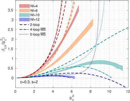
Figure 1: Comparison of the step-scaling functions for $N_{f}=4$, 6, 10 and 12 using the $c=0.300$ scheme with scale change $s=2$. In addition we show the perturbative predictions for the same scale change at 2-loop (universal) as well as 4- and 5-loop in the $\overline{\textrm{MS}}$ scheme Baikov et al. (2017).

We summarize our findings in Fig. 1 where we present the nonperturbative GF step-scaling functions with $N_{f}=4$ (red), 6 (orange), 10 (green) and 12 (blue) flavors in comparison to perturbative predictions. In the case of the QCD-like systems with four or six flavors, our nonpertubative results indicate that the $\beta$ function runs substantially slower than predicted by perturbation theory. In the case of the conformal $N_{f}=12$ system, perturbative results at 3- and 4-loop in the $\overline{\textrm{MS}}$-scheme show a qualitatively and quantitatively similar result as our nonperturbative prediction. However, the 5-loop $\overline{\textrm{MS}}$-result is not a “small correction” to the 4-loop $\overline{\textrm{MS}}$-result. The 5-loop result does not exhibit an IRFP but the poor convergence of the perturbative series makes any prediction for $g^{2}\gtrsim 4.0$ questionable. The (near)conformal $N_{f}=10$ is qualitatively similar to the 3- and 4-loop $\overline{\textrm{MS}}$-predictions but quantitatively the predicted values for the IRFP are rather different. Again the 5-loop result is off, showing a very rapid increase for $g_{c}^{2}>8.5$.

This paper is organized as follows: In Section II we describe the details of our calculations starting with our lattice simulations and the gradient flow measurements. Moreover the definition of the step-scaling $\beta$-function is summarized and the steps of our analysis procedure are given. Our numerical results are presented for SU(3) with six fundamental flavors in Sec. III and for SU(3) with four fundamental flavors in Sec. IV. We discuss our findings in Sec. V where we also compare our results to perturbative predictions, as well as nonperturbative results by the Lattice Higgs collaboration for $N_{f}=4$ resolving the effect of different choices for the scale change $s$. Subsequently we close with a brief summary.

II Details of our Calculation

II.1 Lattice Simulations

As in our previous studies of SU(3) gauge systems with $N_{f}=2$ Hasenfratz and Witzel (2020), 10 Hasenfratz et al. (2019a, 2020) or 12 Hasenfratz et al. (2019a, b) fundamental fermions, we choose the tree-level improved Symanzik (Lüscher-Weisz) gauge action Lüscher and Weisz (1985a, b) and Möbius domain wall fermions (MDWF) Brower et al. (2017) (domain wall height $M_{5}=1.0$, Möbius parameters $b_{5}=1.5$, $c_{5}=0.5$) with three levels of stout-smearing Morningstar and Peardon (2004) ($\varrho=0.1$) for the fermion action. Dynamical gauge field configurations were generated using the hybrid Monte Carlo (HMC) Duane et al. (1987) updating algorithm as implemented in GRID Boyle et al. (2015). We set the fermion mass $am_{f}=0.0$ and choose anti-periodic boundary conditions (BC) for the fermions in all four space-time directions but periodic BC for the gauge field. After thermalization, gauge field configurations are saved every five trajectories and each trajectory has a length of $\tau=2$ molecular dynamic time units (MDTU). Our simulations are performed on $(L/a)^{4}$ hypercubic volumes.

We choose $L/a=$ 8, 10, 12, 16, 20, 24, 32, 40, and calculate the step-scaling function with scale change $s=2$, i.e. we consider volume pairs $(8\to 16)$, $(10\to 20)$, … $(20\to 40)$. We perform simulations using bare gauge couplings $\beta\equiv 6/g_{0}^{2}\in\{$8.50, 7.00, 6.00, 5.20, 4.80, 4.50, 4.30, 4.20, 4.15, 4.10, 4.05$\}$ for $N_{f}=6$ and $\beta\in\{$8.50, 7.00, 6.00, 5.20, 4.80, 4.50, 4.30, 4.25, 4.20$\}$ for $N_{f}=4$. We note however that the strongest couplings are not simulated for all volumes. The goal is to cover (approximately) the same range in the finite volume renormalized couplings on each volume pair, while keeping the system in the small volume deconfined regime. At the same bare coupling, larger volumes reach larger values of the renormalized coupling and might even transit to the confining regime. We monitor the emergence of confinement by computing Polyakov loops. The bare coupling values listed above for the $N_{f}=6$ system correspond to the deconfined regime on all volumes. However, according to the Polyakov loop data, the $N_{f}=4$ system transitions to the confined regime on the largest volumes. On $L/a=40$ volume the strongest coupling we use is $\beta=4.30$ for $N_{f}=6$ and $\beta=4.60$ for $N_{f}=4$. Details of the generated gauge field ensembles including the number of thermalized measurements are shown in Table LABEL:Tab.Nf6_nZS_ZS for $N_{f}=6$ and in Table LABEL:Tab.Nf4_nZS_ZS for $N_{f}=4$ in Appendix A. On the small volumes we typically accumulate 1200 MDTU, but we use lower statistics on the larger volumes. The largest and numerically most expensive $40^{4}$ ensembles have about 200 thermalized MDTU each. Simulations with $\beta>4.20$ are performed using $L_{s}=12$ for the extent of the fifth dimension of domain wall fermions, while $L_{s}=16$ is chosen for $\beta\leq 4.20$. As demonstrated in our previous work Hasenfratz et al. (2019a, 2020, b), this choice ensures that the residual chiral symmetry breaking present for DWF expressed as the residual mass $am_{\text{res}}$ remains sufficiently small, less than $10^{-5}$. The good chiral properties of MDWF protect our zero mass simulations from effects due to nonzero topological charges. Further the simulated gauge fields are sufficiently smooth and we do not observe any topological artifacts like those that contaminated our $N_{f}=10$ simulations Hasenfratz and Witzel (2021).

II.2 Gradient Flow Measurements

Gradient flow measurements are performed on configurations separated by 10 MDTU on all available gauge field configurations. These measurements are carried out using Qlua Pochinsky (2008). In total we perform three sets of gradient flow measurements choosing different actions for the kernel. Specifically we obtain data for Wilson (W), Symanzik (S), and Zeuthen (Z) Sint and Ramos (2015); Ramos and Sint (2016) flow, determining three operators, Wilson plaquette (W), Symanzik (S) and clover (C) to estimate the energy density $\langle E(t)\rangle$ as a function of the gradient flow time $t$.

We use the standard definition of the finite volume gradient flow coupling $g_{GF}^{2}(t;L,\beta)$ Fodor et al. (2012),

$$g^{2}_{GF}(t;L,\beta)=\frac{128\pi^{2}}{3(N^{2}-1)}\frac{1}{C(t,L/a)}\left\langle t^{2}E(t)\right\rangle,$$ (1)

where the constants in front have been chosen to match the perturbative 1-loop result in the $\overline{\textrm{MS}}$ scheme Lüscher (2010) ($N=3$ for the SU(3) gauge group). $C(t,L/a)$ is a perturbatively computed tree-level improvement term Fodor et al. (2014). When analyzing data without tree-level improvement, we replace $C(c,L/a)$ by $1/(1+\delta(t/L^{2}))$ to compensate for zero modes of the gauge field in periodic volumes Fodor et al. (2012).

II.3 Step-scaling $\beta$ Function

When defining the finite volume step-scaling function the flow time $t$ is connected to the lattice size $L$ as

$$t=(cL)^{2}/8.$$ (2)

The parameter $c$ defines the specific finite volume renormalization scheme. For a scale change $s$, the gradient flow step-scaling $\beta$ function Fodor et al. (2012) is given by

$$\beta_{c,s}(g^{2}_{c};L,\beta)=\frac{g^{2}_{c}(sL;\beta)-g^{2}_{c}(L;\beta)}{\log\;s^{2}}\,,$$ (3)

where $g_{c}^{2}(L,\beta)=g^{2}_{GF}(t=(cL)^{2}/8;L,\beta)$. Since the renormalized coupling $g^{2}_{c}$ is defined at a bare coupling $\beta$, it is contaminated by cutoff effects. Hence an extrapolation to the infinite cutoff continuum limit is required. In the case of the step-scaling function this corresponds to taking $t/a^{2}\to\infty$, or equivalently $L/a\to\infty$. At a fixed value of $g^{2}_{c}$ we thus tune the bare coupling toward the Gaussian fixed point i.e. $g_{0}^{2}=6/\beta\to 0$ as $L/a$ increases. Practically simulations are performed on a limited set of lattice volumes. We compensate for that by simulating at many different values of the bare coupling $\beta$. Combining simulations at different bare coupling, we cover the investigated range of the renormalized coupling and take the $L/a\to\infty$ continuum limit of the step-scaling $\beta_{c,s}(g^{2}_{c};L)$ function at fixed $g_{c}^{2}$. As result we obtain the continuum step-scaling $\beta$-function $\beta_{c,s}(g_{c}^{2})$ in the renormalization scheme $c$.

The specific steps of our analysis are as follows:

1. We start by calculating discrete $\beta_{c,s}(g_{c}^{2};L)$ functions as defined in Eq. (3) for all volume pairs with a scale change of $s=2$.

2. For each volume pair we next interpolate these discrete $\beta_{c,s}(g_{c}^{2};L)$ functions using a polynomial ansatz motivated by the perturbative expansion

   $$\beta_{c,s}(g_{c}^{2};L)=\sum_{i=0}^{n}b_{i}g_{c}^{2i}.$$ (4)

   In practice we observe that $n=3$ is sufficient for a good description of our data over the full range in $g_{c}^{2}$ covered by our simulations. When using the tree-level normalization (tln), discretization effects at weak coupling are sufficiently small, hence we constrain the intercept $b_{0}=0$. We fit $b_{0}$ however when analyzing data without tln. After the interpolation, we have finite volume discrete step-scaling functions $\beta_{c,s}(g_{c}^{2};L)$ at continuous values of $g_{c}^{2}$.

3. We take the infinite volume continuum limit by extrapolating the interpolated $\beta_{c,s}(g_{c}^{2};L)$ functions at fixed $g^{2}_{c}$ values. To check for consistency, we explore different choices for the fit ansatz. In particular we perform a quadratic fit to all volume pairs and a linear fit to the largest three volume pairs.

4. The continuum result $\beta_{c,s}(g_{c}^{2})$ should be free of discretization effects but may depend on the renormalization scheme $c$ and the choice of the scale change $s$. Further we need to check for possible systematic effects due to the choice of gradient flow/operators or the use of tln.

II.4 Data Analysis

To distinguish different flow and operator combinations in our analysis, we introduce the shorthand notation [flow][operator] (indicated by the first capital letters) and prefix “n” when including the tree-level improvement term $C(c,L/a)$ in our analysis. As we will detail below, our preferred analysis uses $O(a^{2})$ improved combination of Zeuthen flow with Symanzik operator to which we refer as “ZS” without tree-level improvement and “nZS” with tree-level improvement. The statistical data analysis presented in the following sections is performed using the $\Gamma$-method Wolff (2004) which estimates and accounts for autocorrelations. Table LABEL:Tab.Nf6_nZS_ZS and LABEL:Tab.Nf4_nZS_ZS list the renormalized couplings at our three chosen renormalization schemes $c=0.300$, 0.275 and 0.250 together with the estimated autocorrelations times for our preferred analysis for $N_{f}=6$ and 4, respectively. In the following, we present our analysis for $c=0.300$ but for completeness show plots corresponding to $c=0.275$ and $0.250$ in the Appendix LABEL:Sec.c0275_c0250.

Figure 2: Discrete step-scaling $\beta$-function for $N_{f}=6$ in the $c=0.300$ gradient flow scheme for our preferred nZS (left) and ZS (right) data sets. The symbols in the top row show our results for the finite volume discrete $\beta$ function with scale change $s=2$. The dashed lines with shaded error bands in the same color of the data points show the interpolating fits. We consider two continuum limits: a linear fit (black line with gray error band) in $a^{2}/L^{2}$ to the three largest volume pairs and a quadratic fit to all volume pairs (black dash-dotted line). The $p$-values of the continuum extrapolation fits are shown in the plots in the second row. Further details of the continuum extrapolation at selected $g_{c}^{2}$ values are presented in the small panels at the bottom where the legend lists the extrapolated values in the continuum limit with $p$-values in brackets. Only statistical errors are shown.

III SU(3) with six flavors

Starting from the renormalized couplings shown in Table LABEL:Tab.Nf6_nZS_ZS we calculate the discrete step-scaling function, $\beta_{c,s}(g_{c}^{2};L,\beta)$, (Eq. (3)) for our five volume pairs with scale change $s=2$ and renormalization scheme $c=0.3$: $8\to 16$, $10\to 20$, $12\to 24$, $16\to 32$, and $20\to 40$. These quantities for Zeuthen flow and Symanzik operator (ZS) are shown in the top row panels of Fig. 2 as colored symbols. Plots on the left show our analysis for the tree-level improved combination, whereas plots on the right show the same flow-operator combination without tree-level improvement. Deviations between the various volume pairs indicate cutoff effects. Even for our $O(a^{2})$ improved ZS combination, the tree-level improvement further reduces discretization effects resulting in data for different volume pairs to sit on top of each other. Quite remarkably, within our statistical errors, volume dependence is observable only for $g^{2}_{GF}\gtrsim 6$ when considering the nZS data set. Similar analysis for schemes $c=0.275$ and 0.250 is included in Appendix LABEL:Sec.c0275_c0250.

Next we perform a polynomial interpolation of these data points for any given volume pair to obtain the discrete step-scaling function for continuous values of the renormalized coupling $g_{c}^{2}$. As can be seen by the results for the interpolating fits presented in Tab. LABEL:Tab.interpolationsNf6, a polynomial of degree three is sufficient to describe our data well. As mentioned above, we constrain the intercept to be zero in case of tree-level improved operators because discretization effects are sufficiently small. The corresponding interpolation curve is shown in the top row plots of Fig. 2 by the shaded band in the same color as the data points.

The final step is the continuum limit extrapolation. Taking the results of the previous interpolation, we have data at continuous values of $g_{c}^{2}$ for five different volume pairs. Here we consider two ansätze for the fit:

• “linear” refers to the extrapolation of the three largest volume pairs $12\to 24$, $16\to 32$, and $20\to 40$ using a linear ansatz in $(a/L)^{2}$. The resulting continuum limit values are shown by the solid black line with gray error band in the top row plots of Fig. 2 and the corresponding $p$-values as a function of $g_{c}^{2}$ are presented in the second row plots below.

• “quadratic” uses all five volume pairs and the fit is performed with a quadratic ansatz in $(a/L)^{2}$. The central value of the resulting continuum limit as well as the corresponding $p$-values are shown by a black dash-dotted line.

The excellent agreement between linear and quadratic extrapolation fits for both nZS and ZS analyses for all three renormalization schemes $c$ is apparent. The predicted continuum limits fall into the combined 1-sigma error bands. Further details on the continuum limit extrapolation are demonstrated in the four lowest panels of Fig. 2 where we show the detailed continuum extrapolation at four selected values of $g_{c}^{2}$ across the range where we have performed simulations. We would like to emphasize that these extrapolations for our $N_{f}=6$ data set have good $p$-values over the entire range in $g_{c}^{2}$ for both analyses and all three $c$-values. At all three $c$-values we also observe a clear improvement due to using the tree-level normalization.

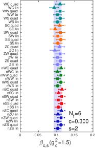
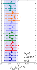
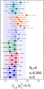
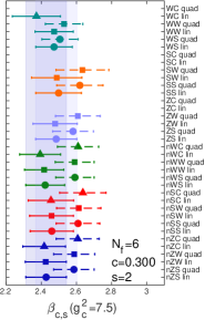
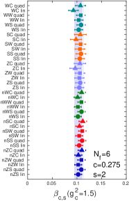
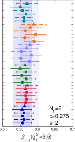
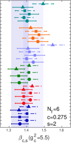
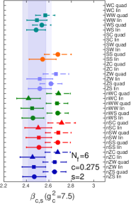
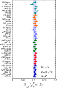
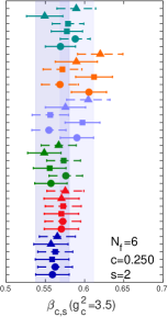
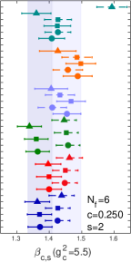
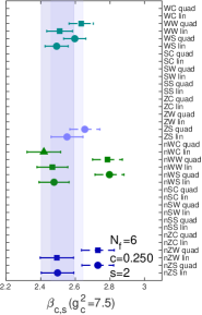
Figure 3: Systematic effects on the $N_{f}=6$ results for $\beta_{c,s}(g_{c}^{2})$ due to tree-level improvement and different flows and operators. In all cases we obtain the continuum limit considering a linear extrapolation to the three largest volume pairs and a quadratic extrapolation to all volume pairs. The columns show our continuum limit results at selective $g_{c}^{2}=1.5$, 3.5, 5.5, and 7.5; the rows correspond to renormalization schemes $c=0.300$, 0.275, 0.250. Open symbols indicate extrapolations with a $p$-value below 5%. The vertical shaded bands highlight our preferred (n)ZS analysis.

We repeat our analysis using the additional flow/operator combinations we have investigated in order to check for possible systematic effects. In total we have performed 18 different analyses considering Zeuthen, Wilson, and Symanzik gradient flow and each time determining the energy density $E(t)$ using the Wilson, Symanzik, and clover operator. Further we carry out each analysis with and without the use of the tree-level normalization. Using again four representative values of $g_{c}^{2}=1.5$, 3.5, 5.5, and 7.5 we show in Fig. 3 comparison plots for the continuum limit values obtained for these 18 different analyses each time performing a linear extrapolation to our three largest volume pairs and a quadratic extrapolation to all five volume pairs. The plots in the top row show comparisons for $c=0.300$, in the middle row for $c=0.275$ and in the bottom row for $c=0.250$, whereas the columns align plots with $g_{c}^{2}=1.5$, 3.5, 5.5, and 7.5. In each plot our preferred analyses, linear continuum extrapolation for nZS and ZS, are highlighted by the shaded blue bands. Alternative analysis based on Zeuthen flow are shown with blue symbols, whereas we use green symbols for Wilson flow and red symbols for Symanzik flow. As we have also observed in our determinations of the step-scaling $\beta$ function for SU(3) with $N_{f}=10$ Hasenfratz et al. (2020) and $N_{f}=12$ Hasenfratz et al. (2019a, b), the reach in $g_{c}^{2}$ depends on the flow-operator combination. In particular when using the clover operator only a shorter range in $g_{c}^{2}$ is covered. This explains “missing” data points for some analysis in the $g_{c}^{2}=7.5$ panels.

Looking at renormalization schemes $c=0.300$ and $c=0.275$ we observe that all analyses have overlapping error bars with the ones we prefer (nZS and ZS) highlighted by the blue bands. In the case of $c=0.250$ we count in total three outliers and note that only less than half of our analysis reach $g_{c}^{2}=7.5$. This suggests $g_{c}^{2}=7.5$ is a bit too large for $c=0.250$ and that systematic effects on our data set slightly increase for decreasing $c$ value.

In the following we use the envelope covering both of our preferred nZS and ZS analysis to quote our final result accounting in addition of statistical uncertainties also for systematic effects. These are shown in Fig. 6, further discussion is, however, postponed to Sec. V.

IV SU(3) with four flavors

Figure 4: Discrete step-scaling $\beta$-function for $N_{f}=4$ in the $c=0.300$ gradient flow scheme for our preferred nZS (left) and ZS (right) data sets. The symbols in the top row show our results for the finite volume discrete $\beta$ function with scale change $s=2$. The dashed lines with shaded error bands in the same color of the data points show the interpolating fits. We consider two continuum limits: a linear fit (black line with gray error band) in $a^{2}/L^{2}$ to the three largest volume pairs and a quadratic fit to all volume pairs (black dash-dotted line). The $p$-values of the continuum extrapolation fits are shown in the plots in the second row. Further details of the continuum extrapolation at selected $g_{c}^{2}$ values are presented in the small panels at the bottom where the legend lists the extrapolated values in the continuum limit with $p$-values in brackets. Only statistical errors are shown.

Our analysis for $N_{f}=4$ proceeds following the same steps as for $N_{f}=6$. We list the renormalized couplings for our preferred (n)ZS analyses in Tab. LABEL:Tab.Nf4_nZS_ZS. These values are the input to determine the discrete step-scaling function $\beta_{c,s}$ shown by the colored symbols in Fig. 4 for the renormalization scheme $c=0.300$ and in Appendix LABEL:Sec.c0275_c0250 for schemes $c=0.275$ and 0.250. To interpolate theses data points in $g_{c}^{2}$ we again use a third order polynomial and constrain the intercept to vanish when using tln. The outcome of these interpolation fits are summarized in Tab. LABEL:Tab.interpolationsNf4. Subsequently, we perform the continuum limit extrapolation using the interpolating curves for all five volume pairs which are continuous in $g_{c}^{2}$. To check for systematic effects, we again consider a linear fit in $a^{2}/L^{2}$ to the three largest volume pairs as well as a quadratic fit in $a^{2}/L^{2}$ using all five volume pairs. Using the same convention as for $N_{f}=6$, the linear (quadratic) fits are shown by a solid black line with gray error band (a dash-dotted black line) in Figs. 4. The overall quality ($p$-value) of the fits is very good and the resulting continuum limits are very close to each other and fall mostly within the $1\sigma$ statistical error band.

Repeating the analysis for our additional data obtained with different operators to estimate the energy density or different kernels to perform the gradient flow, we compare again a total of 18 different analyses as is shown in Fig. 5 for representative values of $g_{c}^{2}=1.5$, 3.0, 4.5, and 6.0. Similar to the case of six fundamental flavors, we do not observe large variations and use the envelope of ZS and nZS to account for systematic effects. Our final result for $N_{f}=4$ is finally presented in Fig. 6.

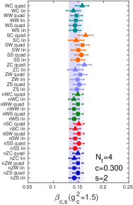
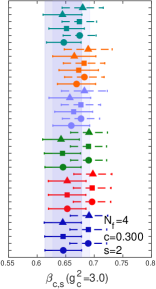
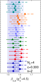
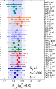
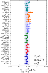
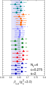
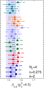
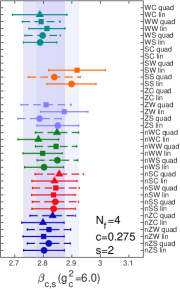
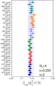
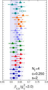
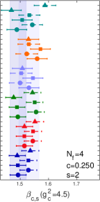
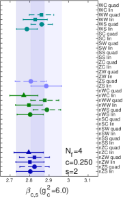
Figure 5: Systematic effects on the $N_{f}=4$ results for $\beta_{c,s}(g_{c}^{2})$ due to tree-level improvement and different flows and operators. In all cases we obtain the continuum limit considering a linear extrapolation to the three largest volume pairs and a quadratic extrapolation to all volume pairs. The columns show our continuum limit results at selective $g_{c}^{2}=1.5$, 3.0, 4.5, and 6.0; the rows correspond to renormalization schemes $c=0.300$, 0.275, 0.250. Open symbols indicate extrapolations with a $p$-value below 5%. The vertical shaded bands highlight our preferred (n)ZS analysis.

V Discussion

V.1 Comparison to perturbative predictions

Figure 6 shows our final results for step-scaling $\beta$-function for SU(3) with $N_{f}=6$ (left) or $N_{f}=4$ (right) fundamental flavors. In comparison to our nonperturbative results for the renormalization schemes $c=0.300$ (top), 0.275 (center), and 0.250 (bottom) we show perturbative predictions. In red the scheme independent results at 1-loop (solid line) and 2-loop (dashed line) are shown, purple crosses denote the 3-loop result in the gradient flow scheme Harlander and Neumann (2016), while the 3-loop (dots), 4-loop (dashed-dotted line), and 5-loop (dotted line) in orange show predictions in the $\overline{\textrm{MS}}$ scheme Baikov et al. (2017); Ryttov and Shrock (2016b).

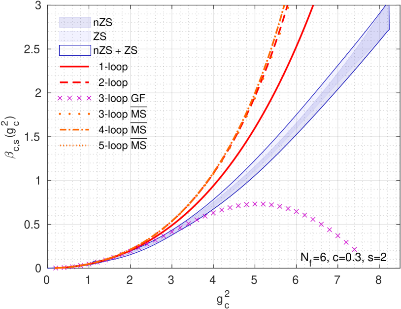
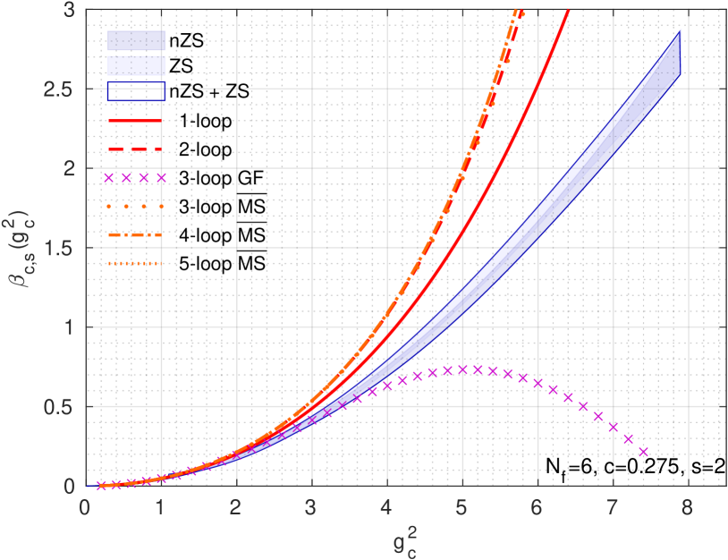
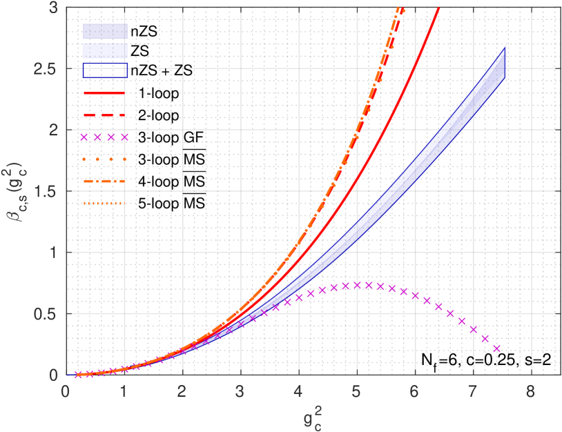
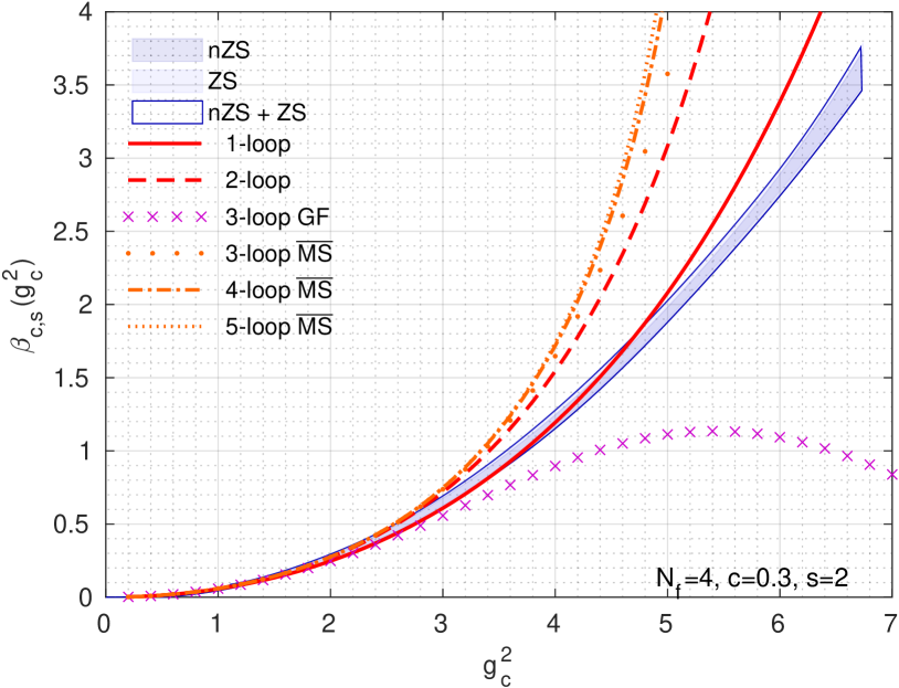
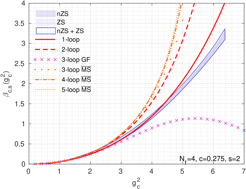
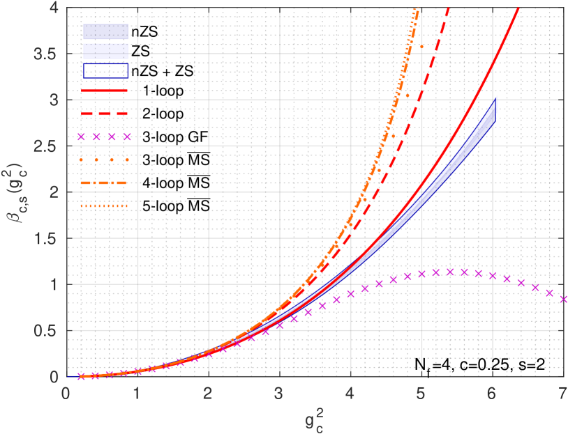
Figure 6: Comparison of our final $N_{f}=6$ (left) and $N_{f}=4$ (right) continuum results obtained from our preferred (n)ZS data set for $c=0.300$ (top), 0.275 (middle), and 0.250 (bottom) to universal 1- and 2-loop perturbative predictions (red), 3-loop perturbative predictions in the gradient flow scheme (purple) and 3-, 4-, and 5-loop $\overline{\textrm{MS}}$ scheme predictions (orange).

In the case of $N_{f}=6$ the 3-loop GF prediction follows our nonperturbative prediction to about $g_{c}^{2}\sim 3.5$ For stronger coupling, however, the 3-loop GF prediction shows a qualitatively different behavior: it turns around pointing to an IRFP. That behavior appears to be common to 3-loop GF for all flavor numbers and may suggest poor convergence of the GF perturbative series. On the other hand, the $\overline{\textrm{MS}}$ predictions show good convergence; the 2 - 5 loop values are very close throughout the investigated $g^{2}$ regime. Notably, our nonperturbative results exhibits a noticeably slower running of the $\beta$-function even than the 1-loop perturbative prediction.

For the system with $N_{f}=4$ flavors our nonperturbative result happens to follow the universal 1-loop prediction up to $g_{c}^{2}\sim 4.5$, while again 2-loop and 3- to 5-loop in the $\overline{\textrm{MS}}$ scheme predict a faster running compared to our results. Similar to the case of $N_{f}=6$ flavors, the 3-loop GF result shows a different qualitatively behavior deviation from our nonperturbative result at about $g_{c}^{2}\sim 3$.

V.2 Comparison to other nonperturbative determinations

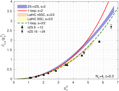
Figure 7: Comparison of our $N_{f}=4$ continuum results obtained from our preferred (n)ZS data set for $c=0.300$ to the non-perturbative results obtained by the Lattice Higgs Collaboration (LatHC) Fodor et al. (2012, 2014). While our results are based on the scale change $s=2$, LatHC uses $s=3/2$.

To the best of our knowledge, no nonperturbative results on the RG $\beta$ function have been reported to date for the SU(3) gauge system with $N_{f}=6$ flavors, although $N_{f}=6$ has been considered to determine e.g. the $S$-parameter Appelquist et al. (2011). For $N_{f}=4$ the Lattice Higgs Collaboration (LatHC) has presented two results based on analyzing gauge field configurations generated with Symanzik gauge action and staggered fermions. They use Symanzik flow and the clover operator and analyze their data without tree-level normalization Fodor et al. (2012) and with tree-level normalization Fodor et al. (2014). In both analyses a scale change $s=3/2$ is used and we refer to their analysis as SSC and nSSC, respectively.

For the fast running $N_{f}=4$ system, the choice of the scale change $s$ has a significant impact on the step scaling function at large coupling. In Fig. 7 we compare our nonperturbative results and the corresponding $s=2$ 1-loop perturbative line to the LatHC results and the corresponding $s=1.5$ perturbative line. In both cases the nonperturbative results follow the 1-loop values up to $g^{2}\approx 5$, suggesting consistency between the numerical predictions.

Given the difference in $s$ a direct comparison between our determination and the determination by LatHC is hence not meaningful. Unfortunately, our existing lattice volumes do not allow to perform a full, alternative analysis using $s=3/2$. Out of the eight different $(L/a)^{4}$ volumes simulated only two volume pairs with $s=3/2$ can be formed, $8\to 12$ and $16\to 24$, which is insufficient to take a meaningful continuum limit. Since our nZS analysis for $s=2$ exhibits very small cutoff effects and different volumes sit on top of each other, we can, however, demonstrate consistency by adding the values of the corresponding finite volume step-scaling function to the plot (black triangles and stars). The symbols for these finite volume step-scaling function indeed sit on top of the LatHC prediction and imply perfect consistency of both results.

V.3 Comparison of different $N_{f}$ = 4, 6, 10, 12

Finally we return to Fig. 1 where we show our newly obtained results for $N_{f}=4$ and 6 in comparison to our published results for $N_{f}=10$ and 12. As we have already discussed in the Introduction, all step scaling functions run slower than perturbatively predicted. Existing data for $N_{f}=2$ suggest the same is true for smaller $N_{f}$ as well. In addition, the GF scheme 3-loop perturbative $\beta$ function shows poor convergence in the numerically interesting strong coupling regime. These observations underline the necessity to use fully nonperturbative running when comparing lattice data to continuum values, like the matching renormalization group $Z$ factors of matrix elements.

VI Summary

In this paper we continued our quest to map the renormalization group $\beta$ function of SU(3) gauge theories with no fermions to the conformal regime, $N_{f}=0-12$. As Fig. 1 illustrates the GF step scaling function approach can predict the nonperturbative $\beta$ function from the weak coupling regime where perturbation theory is applicable to strong coupling where chiral symmetry breaking blocks its applicability ($N_{f}\leq 6$), or to the occurrence of a bulk phase transition that prevents the investigation of stronger couplings ($N_{f}\geq 8$). Once our ongoing $N_{f}=8$ and $N_{f}=0$ studies are complete, all even flavor numbers have been considered. To go beyond the presently accessible range in the QCD-like systems we need to extend the simulations to the confining regime where finite fermion mass will be required. Within the conformal window the biggest challenge is the bulk phase transition that is possibly avoidable, or at least controllable, by improving the action by e.g. including unphysical Pauli-Villars bosons Hasenfratz et al. (2021). These studies are among our future plans.

Since the step-scaling function approach is justified only in the chirally symmetric small volume regime, it cannot be applied once chiral symmetry breaking introduces an infrared scale. In a forthcoming paper we analyze the data using the continuous $\beta$ function approach to demonstrate the consistency between the two methods. That opens the possibility to determine the non-perturbative $\beta$ function from the perturbative ultraviolet to the strongly coupled infrared regimes.

Appendix A Renormalized couplings $g_{c}^{2}$ and details of the polynomial interpolation

Table 1: Details of our preferred analysis for $N_{f}=6$ based on Zeuthen flow and Symanzik operator. For each ensemble specified by the spatial extent $L/a$ and bare gauge coupling $\beta$ we list the number of measurements $N$ as well as the renormalized couplings $g_{c}^{2}$ for the analysis with (nZS) and without tree-level improvement (ZS) for the three renormalization schemes $c=0.300$, 0.275 and 0.250. In addition the integrated autocorrelation times estimated using the $\Gamma$-method Wolff (2004) are listed in units of 10 MDTU.

			$c=0.300$			$c=0.275$			$c=0.250$
$L/a$	$\beta$	$N$	$g_{c}^{2}$(nZS)	$g_{c}^{2}$(ZS)	$\tau_{\text{int}}$	$g_{c}^{2}$(nZS)	$g_{c}^{2}$(ZS)	$\tau_{\text{int}}$	$g_{c}^{2}$(nZS)	$g_{c}^{2}$(ZS)	$\tau_{\text{int}}$
8	8.50	631	1.0638(19)	1.1180(20)	0.53(8)	1.0584(15)	1.1376(17)	0.52(8)	1.0524(12)	1.1713(13)	0.50(8)
8	7.00	631	1.4641(29)	1.5388(30)	0.61(10)	1.4542(23)	1.5630(25)	0.58(9)	1.4429(18)	1.6058(20)	0.56(8)
8	6.00	631	1.9748(38)	2.0754(40)	0.58(9)	1.9540(29)	2.1001(31)	0.50(6)	1.9308(23)	2.1489(25)	0.47(5)
8	5.20	631	2.7586(54)	2.8991(57)	0.51(6)	2.7161(43)	2.9192(46)	0.48(5)	2.6693(33)	2.9709(37)	0.45(5)
8	4.80	631	3.4835(73)	3.6610(77)	0.57(8)	3.4154(62)	3.6708(67)	0.61(10)	3.3403(51)	3.7176(56)	0.63(10)
8	4.50	631	4.403(10)	4.627(11)	0.58(9)	4.2933(86)	4.6144(92)	0.57(9)	4.1731(69)	4.6444(76)	0.57(9)
8	4.30	631	5.473(14)	5.752(14)	0.56(8)	5.302(11)	5.698(12)	0.57(8)	5.1135(92)	5.691(10)	0.57(8)
8	4.20	631	6.285(18)	6.605(19)	0.6(1)	6.066(14)	6.520(15)	0.6(1)	5.824(12)	6.481(14)	0.7(1)
8	4.15	631	6.913(25)	7.265(27)	0.8(1)	6.641(21)	7.138(23)	0.8(1)	6.339(17)	7.055(19)	0.8(2)
8	4.10	631	7.764(31)	8.159(32)	0.8(1)	7.418(26)	7.973(28)	0.8(1)	7.031(20)	7.825(23)	0.7(1)
8	4.05	631	9.012(75)	9.471(79)	2.5(7)	8.552(61)	9.191(65)	2.4(7)	8.027(48)	8.933(54)	2.4(7)
10	8.50	631	1.0836(22)	1.1050(23)	0.63(10)	1.0769(19)	1.1073(19)	0.62(10)	1.0696(15)	1.1149(16)	0.62(10)
10	7.00	619	1.5039(30)	1.5336(31)	0.6(1)	1.4905(24)	1.5326(25)	0.58(9)	1.4763(19)	1.5388(19)	0.53(9)
10	6.00	614	2.0336(39)	2.0738(40)	0.51(6)	2.0105(32)	2.0673(33)	0.48(5)	1.9858(26)	2.0699(28)	0.50(4)
10	5.20	625	2.8857(61)	2.9427(63)	0.57(8)	2.8373(49)	2.9175(50)	0.53(7)	2.7863(38)	2.9042(40)	0.50(6)
10	4.80	631	3.6804(92)	3.7530(93)	0.7(1)	3.6037(73)	3.7055(75)	0.7(1)	3.5228(57)	3.6719(60)	0.63(10)
10	4.50	631	4.762(14)	4.856(14)	0.9(2)	4.628(11)	4.759(12)	0.8(2)	4.4888(86)	4.6788(90)	0.8(1)
10	4.30	631	5.955(18)	6.073(18)	0.9(2)	5.763(14)	5.926(15)	0.8(2)	5.563(11)	5.799(12)	0.8(1)
10	4.20	631	6.973(28)	7.110(29)	1.3(3)	6.716(22)	6.906(23)	1.1(2)	6.450(17)	6.723(18)	1.0(2)
10	4.15	601	7.715(25)	7.867(25)	0.8(2)	7.419(21)	7.629(21)	0.7(1)	7.107(17)	7.408(18)	0.7(1)
10	4.10	601	8.694(31)	8.865(32)	0.8(2)	8.337(26)	8.572(26)	0.8(1)	7.956(21)	8.293(22)	0.7(1)
12	8.50	629	1.1018(22)	1.1123(22)	0.63(10)	1.0942(18)	1.1089(18)	0.59(9)	1.0861(14)	1.1074(14)	0.57(9)
12	7.00	606	1.5344(37)	1.5490(37)	0.8(2)	1.5202(30)	1.5406(30)	0.8(1)	1.5049(24)	1.5345(24)	0.7(1)
12	6.00	601	2.0886(43)	2.1085(43)	0.6(1)	2.0650(35)	2.0927(35)	0.60(10)	2.0389(28)	2.0789(29)	0.58(9)
12	5.20	601	3.0271(90)	3.0559(91)	1.1(2)	2.9689(69)	3.0087(70)	0.9(2)	2.9077(53)	2.9648(54)	0.9(2)
12	4.80	601	3.883(12)	3.920(12)	1.1(2)	3.7946(97)	3.8455(98)	1.0(2)	3.7013(75)	3.7739(76)	0.9(2)
12	4.50	603	5.077(20)	5.126(20)	1.4(3)	4.924(15)	4.990(15)	1.3(3)	4.766(11)	4.859(12)	1.1(3)
12	4.30	601	6.410(27)	6.471(27)	1.6(4)	6.188(21)	6.271(21)	1.5(4)	5.959(15)	6.076(16)	1.3(3)
12	4.20	607	7.608(26)	7.680(26)	1.0(2)	7.304(21)	7.402(21)	0.9(2)	6.998(16)	7.135(17)	0.9(2)
12	4.15	620	8.419(38)	8.499(38)	1.6(4)	8.072(30)	8.181(30)	1.5(4)	7.722(23)	7.873(24)	1.4(3)
16	8.50	300	1.1307(42)	1.1341(42)	1.0(3)	1.1216(34)	1.1264(34)	1.0(3)	1.1120(28)	1.1189(28)	0.9(3)
16	7.00	291	1.5822(54)	1.5871(54)	0.9(2)	1.5689(41)	1.5756(41)	0.7(2)	1.5537(31)	1.5634(31)	0.6(1)
16	6.00	291	2.197(11)	2.204(11)	1.6(5)	2.1684(82)	2.1777(83)	1.3(4)	2.1368(57)	2.1501(58)	0.9(3)
16	5.20	281	3.231(16)	3.241(16)	1.6(5)	3.166(13)	3.180(13)	1.4(4)	3.0979(94)	3.1172(95)	1.2(4)
16	4.80	281	4.236(26)	4.249(26)	1.9(7)	4.132(20)	4.150(20)	1.7(6)	4.022(16)	4.047(16)	1.7(6)
16	4.50	281	5.625(29)	5.643(29)	1.5(5)	5.443(22)	5.466(22)	1.3(4)	5.256(16)	5.289(16)	1.0(3)
16	4.30	281	7.341(48)	7.363(48)	2.1(8)	7.040(38)	7.071(38)	1.9(7)	6.742(29)	6.784(29)	1.8(6)
16	4.20	283	8.775(57)	8.801(57)	1.7(6)	8.383(44)	8.419(44)	1.5(5)	7.995(32)	8.045(32)	1.3(4)
16	4.15	272	9.736(72)	9.765(72)	2.3(9)	9.281(54)	9.321(55)	2.0(7)	8.835(42)	8.890(42)	1.9(7)
16	4.10	282	11.093(80)	11.127(80)	2.2(8)	10.550(58)	10.596(58)	1.8(6)	10.023(42)	10.086(43)	1.5(5)
16	4.05	273	13.51(12)	13.55(12)	3(1)	12.801(85)	12.856(85)	2.3(9)	12.128(62)	12.203(62)	1.8(7)
20	8.50	219	1.1408(61)	1.1422(61)	1.5(6)	1.1348(48)	1.1368(48)	1.4(5)	1.1276(36)	1.1306(36)	1.1(4)
20	7.00	224	1.6263(72)	1.6284(73)	1.2(4)	1.6130(49)	1.6159(50)	0.8(2)	1.5972(38)	1.6014(38)	0.7(2)
20	6.00	197	2.282(15)	2.285(15)	1.4(5)	2.251(12)	2.255(12)	1.2(4)	2.2162(87)	2.2219(88)	1.1(3)
20	5.20	197	3.401(21)	3.406(21)	1.7(6)	3.331(17)	3.337(17)	1.7(6)	3.257(13)	3.265(13)	1.5(5)
20	4.80	203	4.546(31)	4.552(31)	1.7(7)	4.422(25)	4.430(25)	1.7(6)	4.295(19)	4.306(19)	1.6(6)
20	4.50	186	6.205(57)	6.213(57)	3(1)	5.974(44)	5.985(44)	3(1)	5.743(34)	5.757(34)	2(1)
20	4.30	192	8.15(12)	8.16(12)	6(3)	7.796(95)	7.810(95)	5(3)	7.445(71)	7.464(71)	5(2)
20	4.20	227	9.786(79)	9.798(79)	2.4(10)	9.318(55)	9.334(55)	1.8(7)	8.858(40)	8.881(40)	1.6(5)
20	4.15	224	11.04(12)	11.06(12)	4(2)	10.476(83)	10.494(83)	3(1)	9.919(55)	9.944(55)	2.5(10)
20	4.10	231	12.59(17)	12.61(17)	6(3)	11.93(13)	11.95(13)	5(3)	11.285(99)	11.314(99)	5(2)
24	8.50	210	1.1629(64)	1.1637(64)	1.6(6)	1.1565(49)	1.1575(49)	1.3(5)	1.1486(33)	1.1501(33)	0.9(3)
24	7.00	206	1.6812(81)	1.6823(81)	1.1(4)	1.6606(66)	1.6620(66)	1.1(3)	1.6391(52)	1.6412(52)	1.0(3)
24	6.00	208	2.389(16)	2.390(16)	2.1(9)	2.349(11)	2.351(11)	1.4(5)	2.3071(78)	2.3100(78)	1.1(4)
24	5.20	207	3.587(42)	3.590(42)	5(3)	3.503(33)	3.506(33)	5(2)	3.415(26)	3.419(26)	4(2)
24	4.80	202	4.865(32)	4.868(32)	2.1(8)	4.713(25)	4.717(25)	2.0(8)	4.561(20)	4.566(20)	1.9(7)
24	4.50	220	6.616(92)	6.620(92)	6(3)	6.371(67)	6.376(68)	6(3)	6.123(46)	6.131(46)	4(2)
24	4.30	215	8.99(13)	9.00(13)	6(3)	8.563(93)	8.570(93)	5(3)	8.141(67)	8.151(67)	4(2)
24	4.20	209	11.09(16)	11.09(16)	7(3)	10.47(12)	10.48(12)	6(3)	9.871(85)	9.883(85)	5(3)
24	4.15	196	12.51(17)	12.52(17)	6(3)	11.77(13)	11.78(13)	6(3)	11.06(10)	11.07(10)	6(3)
32	8.50	190	1.2100(88)	1.2102(88)	2.3(10)	1.1982(69)	1.1985(69)	2.1(9)	1.1858(51)	1.1863(51)	1.8(7)
32	7.00	182	1.749(11)	1.749(11)	1.9(8)	1.7278(86)	1.7283(86)	1.7(7)	1.7049(67)	1.7056(67)	1.5(5)
32	6.00	178	2.513(26)	2.514(26)	3(2)	2.469(20)	2.469(20)	3(1)	2.422(15)	2.423(15)	3(1)
32	5.20	181	3.866(57)	3.867(57)	6(3)	3.777(44)	3.778(44)	6(3)	3.681(33)	3.683(33)	5(2)
32	4.80	201	5.370(36)	5.371(36)	2.0(8)	5.204(29)	5.205(29)	1.9(7)	5.030(23)	5.032(23)	1.7(7)
32	4.50	198	7.63(13)	7.64(13)	11(6)	7.308(88)	7.310(88)	8(4)	6.982(54)	6.985(54)	5(3)
32	4.30	173	10.65(11)	10.65(11)	3(2)	10.092(74)	10.095(74)	3(1)	9.537(52)	9.541(52)	2.1(9)
32	4.20	181	13.06(13)	13.06(13)	4(2)	12.31(10)	12.32(10)	4(2)	11.582(80)	11.587(80)	4(2)
40	8.50	100	1.2209(87)	1.2210(87)	1.9(9)	1.2143(66)	1.2144(66)	1.5(7)	1.2054(50)	1.2056(50)	1.2(5)
40	7.00	98	1.763(18)	1.763(18)	3(2)	1.755(15)	1.755(15)	3(1)	1.741(12)	1.741(12)	2(1)
40	6.00	101	2.682(71)	2.682(71)	8(4)	2.625(55)	2.625(55)	8(4)	2.565(42)	2.565(42)	7(4)
40	5.20	102	4.167(96)	4.167(96)	7(4)	4.061(73)	4.062(73)	6(4)	3.949(53)	3.950(53)	5(3)
40	4.80	102	5.797(58)	5.798(59)	3(2)	5.614(47)	5.615(47)	3(2)	5.420(38)	5.421(38)	3(1)
40	4.50	121	8.77(16)	8.77(16)	6(3)	8.36(13)	8.36(13)	5(3)	7.93(10)	7.93(10)	5(3)
40	4.30	161	12.14(24)	12.15(24)	11(6)	11.48(18)	11.48(18)	10(6)	10.82(13)	10.82(13)

Table 2: Details of our preferred analysis for $N_{f}=4$ based on Zeuthen flow and Symanzik operator. For each ensemble specified by the spatial extent $L/a$ and bare gauge coupling $\beta$ we list the number of measurements $N$ as well as the renormalized couplings $g_{c}^{2}$ for the analysis with (nZS) and without tree-level improvement (ZS) for the three renormalization schemes $c=0.300$, 0.275 and 0.250. In addition the integrated autocorrelation times estimated using the $\Gamma$-method Wolff (2004) are listed in units of 10 MDTU.

			$c=0.300$			$c=0.275$			$c=0.250$
$L/a$	$\beta$	$N$	$g_{c}^{2}$(nZS)	$g_{c}^{2}$(ZS)	$\tau_{\text{int}}$	$g_{c}^{2}$(nZS)	$g_{c}^{2}$(ZS)	$\tau_{\text{int}}$	$g_{c}^{2}$(nZS)	$g_{c}^{2}$(ZS)	$\tau_{\text{int}}$
8	8.50	591	1.0726(19)	1.1273(20)	0.50(6)	1.0652(16)	1.1448(17)	0.49(6)	1.0574(13)	1.1769(14)	0.49(6)
8	7.00	591	1.4792(27)	1.5546(29)	0.48(7)	1.4650(23)	1.5746(25)	0.50(6)	1.4501(18)	1.6139(20)	0.49(6)
8	6.00	591	1.9934(37)	2.0950(39)	0.50(4)	1.9673(30)	2.1144(32)	0.48(4)	1.9397(24)	2.1588(26)	0.46(4)
8	5.20	591	2.8199(62)	2.9636(65)	0.57(8)	2.7642(51)	2.9709(55)	0.56(8)	2.7054(41)	3.0110(46)	0.57(8)
8	4.80	591	3.5794(86)	3.7618(91)	0.7(1)	3.4881(67)	3.7489(72)	0.61(10)	3.3927(50)	3.7760(55)	0.54(8)
8	4.50	591	4.568(11)	4.801(12)	0.62(10)	4.4175(86)	4.7478(92)	0.56(8)	4.2618(66)	4.7432(73)	0.53(8)
8	4.30	591	5.739(16)	6.032(17)	0.6(1)	5.501(13)	5.912(14)	0.61(10)	5.2550(100)	5.849(11)	0.61(10)
8	4.25	591	6.157(26)	6.471(27)	1.1(2)	5.884(20)	6.323(22)	1.0(2)	5.602(15)	6.235(17)	0.9(2)
8	4.20	591	6.675(24)	7.015(26)	0.8(2)	6.357(19)	6.832(21)	0.8(1)	6.029(14)	6.710(16)	0.7(1)
10	8.50	591	1.0948(20)	1.1164(20)	0.48(4)	1.0860(16)	1.1167(17)	0.46(4)	1.0769(13)	1.1224(14)	0.45(4)
10	7.00	591	1.5273(33)	1.5575(33)	0.7(1)	1.5099(27)	1.5526(27)	0.6(1)	1.4919(21)	1.5550(22)	0.62(10)
10	6.00	591	2.0844(41)	2.1256(42)	0.51(7)	2.0516(33)	2.1096(34)	0.50(7)	2.0178(27)	2.1033(28)	0.50(7)
10	5.20	591	2.9850(77)	3.0440(79)	0.7(1)	2.9202(59)	3.0027(61)	0.7(1)	2.8528(43)	2.9736(45)	0.56(8)
10	4.80	591	3.886(11)	3.962(11)	0.8(1)	3.7681(85)	3.8746(88)	0.7(1)	3.6493(66)	3.8038(69)	0.7(1)
10	4.50	591	5.068(17)	5.168(18)	0.9(2)	4.872(13)	5.009(13)	0.8(1)	4.6764(87)	4.8744(90)	0.58(8)
10	4.30	591	6.523(36)	6.652(37)	2.0(5)	6.213(26)	6.388(27)	1.6(4)	5.906(18)	6.155(19)	1.3(3)
10	4.25	591	7.029(25)	7.168(26)	0.9(2)	6.676(20)	6.864(21)	0.9(2)	6.327(15)	6.594(16)	0.8(2)
12	8.50	623	1.1213(22)	1.1320(22)	0.62(10)	1.1106(18)	1.1255(18)	0.59(9)	1.0995(14)	1.1211(14)	0.51(6)
12	7.00	606	1.5684(39)	1.5833(39)	0.9(2)	1.5492(31)	1.5699(32)	0.8(2)	1.5289(24)	1.5589(24)	0.8(1)
12	6.00	620	2.1595(54)	2.1800(54)	0.9(2)	2.1243(43)	2.1527(44)	0.8(2)	2.0870(34)	2.1280(34)	0.8(2)
12	5.20	609	3.1609(73)	3.1909(74)	0.6(1)	3.0814(61)	3.1227(61)	0.6(1)	2.9992(47)	3.0581(48)	0.59(9)
12	4.80	861	4.158(11)	4.198(11)	1.0(2)	4.0240(84)	4.0779(85)	0.9(1)	3.8867(62)	3.9630(63)	0.8(1)
12	4.50	626	5.544(18)	5.597(18)	1.1(2)	5.309(14)	5.380(14)	1.0(2)	5.073(10)	5.173(11)	0.9(2)
12	4.30	600	7.300(27)	7.370(27)	1.1(2)	6.913(20)	7.006(20)	1.0(2)	6.533(15)	6.661(15)	0.9(2)
16	8.50	499	1.1556(26)	1.1592(27)	0.6(1)	1.1443(21)	1.1492(21)	0.55(8)	1.1323(17)	1.1393(17)	0.51(8)
16	7.00	481	1.6538(46)	1.6588(46)	0.9(2)	1.6289(33)	1.6359(33)	0.7(1)	1.6031(25)	1.6130(25)	0.6(1)
16	6.00	483	2.3103(71)	2.3173(71)	0.9(2)	2.2650(56)	2.2747(57)	0.8(2)	2.2181(45)	2.2319(45)	0.8(2)
16	5.50	495	2.9172(97)	2.9261(97)	1.1(2)	2.8465(76)	2.8587(77)	1.0(2)	2.7736(61)	2.7909(62)	1.0(2)
16	5.20	482	3.477(13)	3.488(13)	1.3(3)	3.377(10)	3.392(10)	1.2(3)	3.2748(78)	3.2952(78)	1.1(2)
16	4.80	483	4.710(25)	4.724(25)	2.0(6)	4.534(19)	4.553(19)	1.7(4)	4.356(14)	4.383(14)	1.4(4)
16	4.60	489	5.741(32)	5.759(32)	2.4(7)	5.486(24)	5.510(24)	2.1(6)	5.233(18)	5.266(18)	1.8(5)
16	4.50	492	6.537(49)	6.557(50)	3(1)	6.211(32)	6.238(32)	2.3(7)	5.889(21)	5.926(21)	1.6(4)
16	4.30	493	9.070(55)	9.098(55)	2.5(8)	8.473(40)	8.509(40)	2.2(7)	7.901(29)	7.950(29)	1.9(5)
16	4.25	482	10.019(73)	10.049(73)	3(1)	9.319(53)	9.359(53)	3.0(10)	8.653(38)	8.707(38)	2.5(8)
16	4.20	482	11.350(85)	11.385(86)	3(1)	10.489(56)	10.534(56)	2.4(7)	9.677(38)	9.737(38)	1.8(5)
20	8.50	303	1.1827(50)	1.1842(50)	1.2(4)	1.1706(38)	1.1726(39)	1.1(3)	1.1578(29)	1.1608(29)	0.9(2)
20	7.00	303	1.6976(68)	1.6998(68)	1.1(3)	1.6740(57)	1.6769(57)	1.1(3)	1.6491(46)	1.6533(46)	1.1(3)
20	6.00	303	2.4230(80)	2.4260(80)	0.8(2)	2.3765(61)	2.3807(61)	0.7(2)	2.3272(49)	2.3332(49)	0.7(1)
20	5.20	301	3.751(26)	3.756(26)	2.5(9)	3.635(19)	3.642(19)	1.9(7)	3.517(13)	3.526(13)	1.6(5)
20	4.80	306	5.218(51)	5.225(51)	5(2)	5.007(38)	5.015(38)	4(2)	4.792(28)	4.805(28)	3(1)
20	4.65	303	6.119(37)	6.126(37)	2.2(8)	5.841(29)	5.851(29)	2.0(7)	5.560(22)	5.574(22)	1.8(6)
20	4.60	303	6.634(68)	6.643(68)	4(1)	6.286(51)	6.297(51)	3(1)	5.945(37)	5.960(37)	3(1)
20	4.50	305	7.705(89)	7.715(90)	5(2)	7.237(66)	7.250(67)	4(2)	6.785(47)	6.803(47)	4(2)
20	4.30	303	10.882(98)	10.896(98)	4(2)	10.074(73)	10.092(73)	4(2)	9.305(54)	9.329(55)	3(1)
20	4.25	302	12.20(12)	12.21(12)	4(2)	11.232(95)	11.252(95)	4(2)	10.324(76)	10.350(76)	5(2)
24	8.50	201	1.2069(70)	1.2077(70)	1.9(7)	1.1949(56)	1.1960(56)	1.8(7)	1.1818(44)	1.1833(44)	1.6(6)
24	7.00	201	1.781(14)	1.782(14)	3(1)	1.749(11)	1.751(11)	3(1)	1.7172(86)	1.7194(86)	3(1)
24	6.00	201	2.543(23)	2.545(24)	3(1)	2.489(18)	2.491(18)	2(1)	2.433(14)	2.436(14)	2.3(9)
24	5.20	351	4.073(43)	4.075(43)	6(2)	3.931(33)	3.935(33)	5(2)	3.787(24)	3.792(24)	4(2)
24	4.80	577	5.812(57)	5.816(57)	8(3)	5.534(40)	5.539(40)	6(2)	5.261(29)	5.267(29)	5(2)
24	4.50	408	8.726(75)	8.731(75)	5(2)	8.165(55)	8.173(55)	4(2)	7.621(37)	7.631(38)	3(1)
24	4.30	321	12.71(14)	12.72(14)	6(3)	11.70(11)	11.71(11)	6(3)	10.737(80)	10.750(80)	5(2)
32	8.50	121	1.251(10)	1.251(10)	2(1)	1.2374(84)	1.2377(84)	2.0(9)	1.2228(64)	1.2233(64)	1.7(8)
32	7.00	105	1.900(12)	1.900(12)	1.2(5)	1.861(10)	1.862(10)	1.1(5)	1.8214(89)	1.8222(89)	1.1(5)
32	6.00	140	2.732(27)	2.733(27)	3(1)	2.674(21)	2.674(21)	2(1)	2.611(16)	2.612(16)	1.9(9)
32	5.50	152	3.680(63)	3.681(63)	5(3)	3.565(49)	3.566(49)	5(3)	3.445(37)	3.446(37)	5(2)
32	5.20	161	4.595(65)	4.596(65)	4(2)	4.419(52)	4.420(52)	4(2)	4.240(41)	4.241(41)	4(2)
32	4.80	123	6.910(99)	6.912(99)	5(3)	6.545(73)	6.547(73)	4(2)	6.182(50)	6.184(50)	3(2)
32	4.60	171	9.301(94)	9.303(94)	4(2)	8.648(76)	8.650(76)	4(2)	8.027(59)	8.030(59)	4(2)
32	4.50	121	10.930(75)	10.932(75)	3(2)	10.133(65)	10.136(65)	3(2)	9.372(57)	9.376(57)	3(2)
40	8.50	91	1.291(11)	1.291(11)	2(1)	1.2753(98)	1.2754(98)	3(1)	1.2593(78)	1.2595(78)	2(1)
40	7.00	111	1.949(33)	1.949(33)	5(3)	1.914(25)	1.914(25)	4(2)	1.877(18)	1.877(18)	4(2)
40	6.00	121	3.015(35)	3.015(35)	3(2)	2.922(27)	2.922(27)	3(2)	2.828(21)	2.829(21)	3(1)
40	5.20	103	5.014(93)	5.015(93)	7(4)	4.824(70)	4.825(70)	6(3)	4.628(52)	4.629(52)	5(3)
40	4.80	111	8.175(49)	8.176(49)	2(1)	7.649(38)	7.650(38)	1.8(8)	7.150(29)	7.151(29)	1.6(7)
40	4.65	143	10.18(15)	10.18(15)	5(3)	9.49(11)	9.49(11)	5(2)	8.816(78)	8.818(78)	4(2)
40	4.60	135	11.18(20)	11.18(20)	9(5)	10.35(16)	10.35(16)	9(5)	9.55(13)	9.55(13)

	analysis	$c$	d.o.f.	$\chi^{2}$/d.o.f.	$p$-value	$b_{3}$	$b_{2}$	$b_{1}$	$b_{0}$
$8\to 16$	ZS	0.300	7	0.780	0.604	-0.00268(58)	0.0681(70)	-0.110(23)	0.053(20)
$10\to 20$	ZS	0.300	6	0.077	0.998	-0.00319(97)	0.071(11)	-0.076(36)	0.029(30)
$12\to 24$	ZS	0.300	5	0.555	0.734	-0.0002(12)	0.039(14)	0.035(42)	-0.050(34)
$16\to 32$	ZS	0.300	4	0.585	0.673	-0.0016(12)	0.057(16)	-0.024(53)	0.013(46)
$20\to 40$	ZS	0.300	3	1.273	0.282	-0.0018(23)	0.066(27)	-0.070(86)	0.053(72)
$8\to 16$	ZS	0.275	7	0.940	0.474	-0.00195(48)	0.0595(58)	-0.108(19)	0.041(16)
$10\to 20$	ZS	0.275	6	0.093	0.997	-0.00304(82)	0.0681(94)	-0.076(29)	0.027(24)
$12\to 24$	ZS	0.275	5	0.644	0.666	-0.0005(10)	0.042(11)	0.017(34)	-0.035(27)
$16\to 32$	ZS	0.275	4	0.751	0.557	-0.0018(11)	0.059(13)	-0.034(43)	0.019(37)
$20\to 40$	ZS	0.275	3	1.346	0.257	-0.0016(21)	0.063(23)	-0.057(72)	0.041(59)
$8\to 16$	ZS	0.250	7	1.219	0.288	-0.00082(40)	0.0476(47)	-0.109(15)	0.025(14)
$10\to 20$	ZS	0.250	6	0.154	0.988	-0.00278(69)	0.0645(77)	-0.081(23)	0.026(19)
$12\to 24$	ZS	0.250	5	0.780	0.564	-0.00090(88)	0.0459(93)	-0.004(26)	-0.020(21)
$16\to 32$	ZS	0.250	4	0.970	0.423	-0.00196(95)	0.061(11)	-0.042(34)	0.023(29)
$20\to 40$	ZS	0.250	3	1.404	0.239	-0.0014(19)	0.060(20)	-0.045(60)	0.030(48)
$8\to 16$	nZS	0.300	8	1.594	0.121	-0.00158(35)	0.0561(29)	-0.0177(46)	—
$10\to 16$	nZS	0.300	7	0.199	0.986	-0.00251(49)	0.0634(43)	-0.0299(66)	—
$12\to 16$	nZS	0.300	6	0.821	0.553	-0.00176(60)	0.0587(50)	-0.0187(75)	—
$16\to 16$	nZS	0.300	5	0.484	0.788	-0.00134(61)	0.0536(57)	-0.0075(93)	—
$20\to 16$	nZS	0.300	4	1.090	0.359	-0.0003(12)	0.0478(95)	-0.007(13)	—
$8\to 16$	nZS	0.275	8	1.620	0.113	-0.00115(30)	0.0533(25)	-0.0162(38)	—
$10\to 16$	nZS	0.275	7	0.263	0.968	-0.00241(43)	0.0615(36)	-0.0265(53)	—
$12\to 16$	nZS	0.275	6	0.818	0.556	-0.00175(53)	0.0574(42)	-0.0172(61)	—
$16\to 16$	nZS	0.275	5	0.653	0.659	-0.00134(55)	0.0536(49)	-0.0092(77)	—
$20\to 16$	nZS	0.275	4	1.135	0.338	-0.0003(11)	0.0479(81)	-0.006(11)	—
$8\to 16$	nZS	0.250	8	1.560	0.131	-0.00025(27)	0.0487(21)	-0.0130(32)	—
$10\to 20$	nZS	0.250	7	0.409	0.898	-0.00219(37)	0.0591(30)	-0.0232(43)	—
$12\to 24$	nZS	0.250	6	0.807	0.564	-0.00174(45)	0.0563(34)	-0.0165(47)	—
$16\to 32$	nZS	0.250	5	0.907	0.475	-0.00132(48)	0.0534(40)	-0.0105(61)	—
$20\to 40$	nZS	0.250	4	1.154	0.329	-0.00034(93)	0.0480(68)	-0.0055(88)	—

	analysis	$c$	d.o.f.	$\chi^{2}$/d.o.f.	$p$-value	$b_{3}$	$b_{2}$	$b_{1}$	$b_{0}$
$8\to 16$	ZS	0.300	5	0.496	0.779	0.0044(12)	0.035(12)	-0.005(32)	-0.021(24)
$10\to 20$	ZS	0.300	4	0.776	0.540	0.0009(17)	0.076(17)	-0.087(45)	0.051(34)
$12\to 24$	ZS	0.300	3	1.473	0.220	-0.0001(21)	0.080(22)	-0.053(63)	0.015(50)
$16\to 32$	ZS	0.300	4	2.516	0.039	0.0016(32)	0.068(32)	-0.023(87)	0.005(68)
$20\to 40$	ZS	0.300	3	2.015	0.109	-0.0009(47)	0.091(46)	-0.05(13)	0.01(10)
$8\to 16$	ZS	0.275	5	0.589	0.709	0.00403(94)	0.0345(92)	-0.029(25)	-0.015(19)
$10\to 20$	ZS	0.275	4	0.822	0.511	0.0012(15)	0.070(15)	-0.080(38)	0.041(28)
$12\to 24$	ZS	0.275	3	1.731	0.158	0.0003(19)	0.076(19)	-0.054(53)	0.016(41)
$16\to 32$	ZS	0.275	4	2.155	0.071	0.0023(30)	0.061(28)	-0.011(76)	-0.005(58)
$20\to 40$	ZS	0.275	3	1.702	0.164	0.0010(44)	0.073(42)	-0.02(11)	-0.006(85)
$8\to 16$	ZS	0.250	5	0.588	0.709	0.00384(74)	0.0315(72)	-0.056(20)	-0.011(16)
$10\to 10$	ZS	0.250	4	0.906	0.459	0.0015(13)	0.064(12)	-0.078(31)	0.033(23)
$12\to 24$	ZS	0.250	3	2.141	0.093	0.0005(16)	0.072(16)	-0.057(43)	0.018(33)
$16\to 32$	ZS	0.250	4	1.694	0.148	0.0028(28)	0.057(25)	-0.006(66)	-0.008(49)
$20\to 40$	ZS	0.250	3	1.403	0.240	0.0024(41)	0.062(37)	-0.003(96)	-0.013(71)
$8\to 16$	nZS	0.300	6	0.562	0.761	0.00393(57)	0.0498(39)	-0.0005(50)	—
$10\to 20$	nZS	0.300	5	1.079	0.369	0.00339(75)	0.0534(56)	-0.0073(77)	—
$12\to 24$	nZS	0.300	4	1.129	0.341	0.0005(10)	0.0748(75)	-0.028(10)	—
$16\to 32$	nZS	0.300	5	2.015	0.073	0.0019(14)	0.066(11)	-0.015(15)	—
$20\to 40$	nZS	0.300	4	1.515	0.195	-0.0004(20)	0.085(14)	-0.035(19)	—
$8\to 16$	nZS	0.275	6	0.613	0.720	0.00416(48)	0.0476(32)	-0.0005(41)	—
$10\to 20$	nZS	0.275	5	1.097	0.360	0.00345(66)	0.0524(47)	-0.0068(62)	—
$12\to 24$	nZS	0.275	4	1.341	0.252	0.00095(90)	0.0705(63)	-0.0240(84)	—
$16\to 32$	nZS	0.275	5	1.726	0.125	0.0021(13)	0.0640(93)	-0.014(12)	—
$20\to 40$	nZS	0.275	4	1.279	0.276	0.0007(18)	0.076(13)	-0.026(17)	—
$8\to 16$	nZS	0.250	6	0.603	0.728	0.00463(42)	0.0446(27)	-0.0002(33)	—
$10\to 20$	nZS	0.250	5	1.143	0.335	0.00359(58)	0.0508(39)	-0.0061(49)	—
$12\to 24$	nZS	0.250	4	1.685	0.150	0.00136(79)	0.0667(53)	-0.0207(68)	—
$16\to 32$	nZS	0.250	5	1.362	0.235	0.0024(12)	0.0615(79)	-0.013(10)	—
$20\to 40$	nZS	0.250	4	1.061	0.374	0.0017(16)	0.069(11)	-0.019(14)	—

Appendix B Tree-level normalization factors

flow/op.	$L/a$	$C(0.250,L/a)$	$C(0.275,L/a)$	$C(0.300,L/a)$
ZS	40	0.987231	0.981324	0.973551
ZS	48	0.973551	0.981254	0.973510
ZW	40	0.982875	0.977615	0.970391
ZW	48	0.970391	0.978671	0.971310
ZC	40	0.969595	0.966514	0.960929
ZC	48	0.960929	0.970935	0.964718
SS	40	0.984012	0.978590	0.971254
SS	48	0.971254	0.979351	0.971912
SW	40	0.997304	0.989589	0.980385
SW	48	0.980385	0.984379	0.976126
SC	40	0.966420	0.963868	0.958695
SC	48	0.958695	0.969076	0.963151
WS	40	0.997304	0.989589	0.980516
WS	48	0.980516	0.986993	0.978348
WW	40	0.992773	0.985817	0.977312
WW	48	0.977312	0.984379	0.976126
WC	40	0.979219	0.974528	0.967716
WC	48	0.967716	0.976552	0.969470

Appendix C Analyses for $c=0.275$ and $c=0.250$

References

- Kronfeld et al. (2022) Andreas S. Kronfeld et al. (USQCD), “Lattice QCD and Particle Physics,” (2022), arXiv:2207.07641 [hep-lat] .
- Davoudi et al. (2022) Zohreh Davoudi et al., “Report of the Snowmass 2021 Topical Group on Lattice Gauge Theory,” in 2022 Snowmass Summer Study (2022) arXiv:2209.10758 [hep-lat] .
- Narayanan and Neuberger (2006) R. Narayanan and H. Neuberger, “Infinite N phase transitions in continuum Wilson loop operators,” JHEP 0603, 064 (2006), arXiv:hep-th/0601210 [hep-th] .
- Lüscher (2010) Martin Lüscher, “Trivializing maps, the Wilson flow and the HMC algorithm,” Commun.Math.Phys. 293, 899–919 (2010), arXiv:0907.5491 [hep-lat] .
- Lüscher (2010) Martin Lüscher, “Properties and uses of the Wilson flow in lattice QCD,” JHEP 1008, 071 (2010), arXiv:1006.4518 [hep-lat] .
- Fodor et al. (2012) Zoltan Fodor, Kieran Holland, Julius Kuti, Daniel Nogradi, and Chik Him Wong, “The Yang-Mills gradient flow in finite volume,” JHEP 1211, 007 (2012), arXiv:1208.1051 [hep-lat] .
- Lüscher (2014) Martin Lüscher, “Step scaling and the Yang-Mills gradient flow,” JHEP 06, 105 (2014), arXiv:1404.5930 [hep-lat] .
- Hasenfratz and Witzel (2020) Anna Hasenfratz and Oliver Witzel, “Continuous renormalization group function from lattice simulations,” Phys. Rev. D101, 034514 (2020), arXiv:1910.06408 [hep-lat] .
- Fodor et al. (2018a) Zoltan Fodor, Kieran Holland, Julius Kuti, Daniel Nogradi, and Chik Him Wong, “A new method for the beta function in the chiral symmetry broken phase,” EPJ Web Conf. 175, 08027 (2018a), arXiv:1711.04833 [hep-lat] .
- Hasenfratz and Witzel (2019) Anna Hasenfratz and Oliver Witzel, “Continuous function for the SU(3) gauge systems with two and twelve fundamental flavors,” PoS LATTICE2019, 094 (2019), arXiv:1911.11531 [hep-lat] .
- Peterson et al. (2021) Curtis T. Peterson, Anna Hasenfratz, Jake van Sickle, and Oliver Witzel, “Determination of the continuous function of SU(3) Yang-Mills theory,” in 38th International Symposium on Lattice Field Theory (2021) arXiv:2109.09720 [hep-lat] .
- Hasenfratz et al. (2022) Anna Hasenfratz, Christopher J. Monahan, Matthew D. Rizik, Andrea Shindler, and Oliver Witzel, “A novel nonperturbative renormalization scheme for local operators,” in 38th International Symposium on Lattice Field Theory (2022) arXiv:2201.09740 [hep-lat] .
- Dalla Brida et al. (2017) Mattia Dalla Brida, Patrick Fritzsch, Tomasz Korzec, Alberto Ramos, Stefan Sint, and Rainer Sommer (ALPHA), “Slow running of the Gradient Flow coupling from 200 MeV to 4 GeV in QCD,” Phys. Rev. D95, 014507 (2017), arXiv:1607.06423 [hep-lat] .
- Harlander and Neumann (2016) Robert V. Harlander and Tobias Neumann, “The perturbative QCD gradient flow to three loops,” JHEP 06, 161 (2016), arXiv:1606.03756 [hep-ph] .
- Hasenfratz and Schaich (2018) Anna Hasenfratz and David Schaich, “Nonperturbative beta function of twelve-flavor SU(3) gauge theory,” JHEP 02, 132 (2018), arXiv:1610.10004 [hep-lat] .
- Hasenfratz et al. (2019a) A. Hasenfratz, C. Rebbi, and O. Witzel, “Nonperturbative determination of functions for SU(3) gauge theories with 10 and 12 fundamental flavors using domain wall fermions,” Phys. Lett. B798, 134937 (2019a), arXiv:1710.11578 [hep-lat] .
- Hasenfratz et al. (2019b) Anna Hasenfratz, Claudio Rebbi, and Oliver Witzel, “Gradient flow step-scaling function for SU(3) with twelve flavors,” Phys. Rev. D100, 114508 (2019b), arXiv:1909.05842 [hep-lat] .
- Hasenfratz et al. (2020) Anna Hasenfratz, Claudio Rebbi, and Oliver Witzel, “Gradient flow step-scaling function for SU(3) with ten fundamental flavors,” Phys. Rev. D 101, 114508 (2020), arXiv:2004.00754 [hep-lat] .
- Chiu (2016) Ting-Wai Chiu, “The -function of gauge theory with massless fermions in the fundamental representation,” (2016), arXiv:1603.08854 [hep-lat] .
- Chiu (2019) Ting-Wai Chiu, “Improved study of the -function of gauge theory with massless domain-wall fermions,” Phys. Rev. D99, 014507 (2019), arXiv:1811.01729 [hep-lat] .
- Fodor et al. (2016) Zoltan Fodor, Kieran Holland, Julius Kuti, Santanu Mondal, Daniel Nogradi, and Chik Him Wong, “Fate of the conformal fixed point with twelve massless fermions and SU(3) gauge group,” Phys. Rev. D94, 091501 (2016), arXiv:1607.06121 [hep-lat] .
- Fodor et al. (2018b) Zoltan Fodor, Kieran Holland, Julius Kuti, Daniel Nogradi, and Chik Him Wong, “Extended investigation of the twelve-flavor -function,” Phys. Lett. B779, 230–236 (2018b), arXiv:1710.09262 [hep-lat] .
- Fodor et al. (2018c) Zoltan Fodor, Kieran Holland, Julius Kuti, Daniel Nogradi, and Chik Him Wong, “The twelve-flavor -function and dilaton tests of the sextet scalar,” EPJ Web Conf. 175, 08015 (2018c), arXiv:1712.08594 [hep-lat] .
- Fodor et al. (2018d) Zoltan Fodor, Kieran Holland, Julius Kuti, Daniel Nogradi, and Chik Him Wong, “Fate of a recent conformal fixed point and -function in the SU(3) BSM gauge theory with ten massless flavors,” PoS LATTICE2018, 199 (2018d), arXiv:1812.03972 [hep-lat] .
- Ryttov and Shrock (2011) Thomas A. Ryttov and Robert Shrock, “Higher-loop corrections to the infrared evolution of a gauge theory with fermions,” Phys. Rev. D83, 056011 (2011), arXiv:1011.4542 .
- Ryttov and Shrock (2016a) Thomas A. Ryttov and Robert Shrock, “Scheme-Independent Series Expansions at an Infrared Zero of the Beta Function in Asymptotically Free Gauge Theories,” Phys. Rev. D94, 125005 (2016a), arXiv:1610.00387 [hep-th] .
- Ryttov and Shrock (2016b) Thomas A. Ryttov and Robert Shrock, “Infrared Zero of and Value of for an SU(3) Gauge Theory at the Five-Loop Level,” Phys. Rev. D94, 105015 (2016b), arXiv:1607.06866 [hep-th] .
- Ryttov and Shrock (2018) Thomas A. Ryttov and Robert Shrock, “Physics of the non-Abelian Coulomb phase: Insights from Padé approximants,” Phys. Rev. D 97, 025004 (2018), arXiv:1710.06944 [hep-th] .
- Hasenfratz (2022) Anna Hasenfratz, “Emergent strongly coupled ultraviolet fixed point in four dimensions with eight Kähler-Dirac fermions,” Phys. Rev. D 106, 014513 (2022), arXiv:2204.04801 [hep-lat] .
- Appelquist et al. (2019) T. Appelquist, R.C. Brower, G.T. Fleming, A. Gasbarro, A. Hasenfratz, X.-Y. Jin, E.T. Neil, J.C. Osborn, C. Rebbi, E. Rinaldi, D. Schaich, P. Vranas, E. Weinberg, and O. Witzel (Lattice Strong Dynamics), “Nonperturbative investigations of SU(3) gauge theory with eight dynamical flavors,” Phys. Rev. D99, 014509 (2019), arXiv:1807.08411 [hep-lat] .
- Baikov et al. (2017) P. A. Baikov, K. G. Chetyrkin, and J. H. Kühn, “Five-Loop Running of the QCD coupling constant,” Phys. Rev. Lett. 118, 082002 (2017), arXiv:1606.08659 [hep-ph] .
- Lüscher and Weisz (1985a) M. Lüscher and P. Weisz, “On-Shell Improved Lattice Gauge Theories,” Commun. Math. Phys. 97, 59 (1985a), [Erratum: Commun. Math. Phys.98,433(1985)].
- Lüscher and Weisz (1985b) M. Lüscher and P. Weisz, “Computation of the Action for On-Shell Improved Lattice Gauge Theories at Weak Coupling,” Phys. Lett. 158B, 250–254 (1985b).
- Brower et al. (2017) Richard C. Brower, Harmut Neff, and Kostas Orginos, “The Möbius domain wall fermion algorithm,” Comput. Phys. Commun. 220, 1–19 (2017), arXiv:1206.5214 [hep-lat] .
- Morningstar and Peardon (2004) Colin Morningstar and Mike J. Peardon, “Analytic smearing of SU(3) link variables in lattice QCD,” Phys. Rev. D69, 054501 (2004), arXiv:hep-lat/0311018 [hep-lat] .
- Duane et al. (1987) S. Duane, A.D. Kennedy, B.J. Pendleton, and D. Roweth, “Hybrid Monte Carlo,” Phys.Lett. B195, 216–222 (1987).
- Boyle et al. (2015) Peter Boyle, Azusa Yamaguchi, Guido Cossu, and Antonin Portelli, “Grid: A next generation data parallel C++ QCD library,” PoS LATTICE2015, 023 (2015), arXiv:1512.03487 [hep-lat] .
- Hasenfratz and Witzel (2021) Anna Hasenfratz and Oliver Witzel, “Dislocations under gradient flow and their effect on the renormalized coupling,” Phys. Rev. D 103, 034505 (2021), arXiv:2004.00758 [hep-lat] .
- Pochinsky (2008) Andrew Pochinsky, “Writing efficient QCD code made simpler: QA(0),” PoS LATTICE2008, 040 (2008).
- Sint and Ramos (2015) Stefan Sint and Alberto Ramos, “On O() effects in gradient flow observables,” PoS LATTICE2014, 329 (2015), arXiv:1411.6706 [hep-lat] .
- Ramos and Sint (2016) A. Ramos and S. Sint, “Symanzik improvement of the gradient flow in lattice gauge theories,” Eur. Phys. J. C76, 15 (2016), arXiv:1508.05552 [hep-lat] .
- Fodor et al. (2014) Zoltan Fodor, Kieran Holland, Julius Kuti, Santanu Mondal, Daniel Nogradi, and Chik Him Wong, “The lattice gradient flow at tree-level and its improvement,” JHEP 09, 018 (2014), arXiv:1406.0827 [hep-lat] .
- Wolff (2004) Ulli Wolff (ALPHA), “Monte Carlo errors with less errors,” Comput.Phys.Commun. 156, 143–153 (2004), arXiv:hep-lat/0306017 [hep-lat] .
- Appelquist et al. (2011) Thomas Appelquist et al. (LSD), “Parity Doubling and the S Parameter Below the Conformal Window,” Phys. Rev. Lett. 106, 231601 (2011), arXiv:1009.5967 [hep-ph] .
- Hasenfratz et al. (2021) Anna Hasenfratz, Yigal Shamir, and Benjamin Svetitsky, “Taming lattice artifacts with Pauli-Villars fields,” Phys. Rev. D 104, 074509 (2021), arXiv:2109.02790 [hep-lat] .
- Anderson et al. (2017) Jonathon Anderson, Patrick J. Burns, Daniel Milroy, Peter Ruprecht, Thomas Hauser, and Howard Jay Siegel, “Deploying rmacc summit: An hpc resource for the rocky mountain region,” Proceedings of PEARC17 8, 1–7 (2017).
- Towns et al. (2014) J. Towns, T. Cockerill, M. Dahan, I. Foster, K. Gaither, A. Grimshaw, V. Hazlewood, S. Lathrop, D. Lifka, G. D. Peterson, R. Roskies, J. R. Scott, and N. Wilkins-Diehr, “Xsede: Accelerating scientific discovery,” Computing in Science & Engineering 16, 62–74 (2014).