Subsonic and supersonic mechanisms in compressible turbulent boundary layers: a perspective from resolvent analysis

Abstract

In this study we isolate the mechanisms that are separately responsible for amplifying the two distinct sets of modes that appear in a linearized Navier–Stokes based model for compressible turbulent boundary layer flows. These two sets of modes are: (i) the subsonic modes that have equivalents in the incompressible flow regime, and (ii) the supersonic modes that do not have such equivalents in the incompressible flow regime. The resolvent analysis framework introduced by McKeon & Sharma (J. Fluid Mech., vol. 658, 2010, pp. 336–382) is used to analyze the linear model, where the non-linear terms of the equations are taken to be a forcing to the linear terms. The most sensitive forcing and correspondingly the most amplified response are then analyzed. We find that, when considering the subsonic response modes, only the solenoidal component of the forcing to the momentum equations can amplify these modes. This is consistent with observations in the literature regarding incompressible flows. Next, when considering the supersonic response modes, we find that these are pressure fluctuations that radiate into the freestream. Within the freestream, these modes closely follow the trends of the inviscid Mach waves. There are three different forcing mechanisms that are found to amplify these modes. First, the forcing to the continuity and energy equations contribute. Second, the dilatational component of the forcing to the momentum equations has a significant role. Finally, although less significant for the resolvent amplification, there is also a contribution from the solenoidal component of the forcing.

Using these identified forcing mechanisms, a decomposition of the forcing to the compressible resolvent operator, i.e. of the non-linear terms of the linearized Navier–Stokes equations, is proposed, that can approximately isolate the subsonic and the supersonic modes. We verify this decomposition of the forcing in turbulent boundary layers both over adiabatic as well as cooled walls, and for a range of Mach numbers. These results are consistent with, and extend, the observations in the literature regarding the solenoidal and the dilatational components of the velocity in compressible turbulent wall-bounded flows.

1 Introduction

We can broadly categorise the flow features that appear in compressible wall-bounded flows as two different kinds: (i) subsonic features that have equivalents in incompressible flows and (ii) supersonic features that have no such equivalents in incompressible flows. In the incompressible regime, an important feature is the coherent structures that appear in the flow and the first identified among these coherent structures are the near-wall streaks (Kline et al., 1967). These structures appear very close to the wall, i.e. in the buffer layer of the flow, and contribute significantly to the turbulent kinetic energy production in this region (Kline et al., 1967; Smits et al., 2011). When considering compressible flows, there is evidence that suggests that the streamwise lengths and the spanwise widths of these structures do not change when compared to incompressible flows (Duan et al., 2011; Lagha et al., 2011). On the other hand, when considering compressible boundary layers over cooled walls, these near wall streaks get longer and wider (Duan et al., 2010). Apart from these near-wall structures, incompressible flows also have the ‘large-scale motions’ (LSMs) that have characteristic length-scales of $2-3\delta$ (where $\delta$ is the boundary layer thickness), and the ‘very-large-scale motions’ (VLSMs) with lengths $10-15\delta$. These structures exist within the logarithmic region of the flow, and their contribution to the turbulent kinetic energy and the Reynolds shear stress increases with Reynolds number (see Smits et al. (2011) and references therein for a review about these structures). When considering compressible flows, there are many studies that have shown the existence of such large-scale structures in these flows, and there is an ongoing debate on how the length scales of these structures change with increasing Mach number and wall-cooling (e.g. Smits et al., 1989; Smits & Dussauge, 2006; Pirozzoli & Bernardini, 2011; Ganapathisubramani et al., 2006; Duan & Martin, 2011; Williams et al., 2018; Bross et al., 2021).

Now let us consider the supersonic features in compressible flows, that have no equivalents in incompressible flows. Here we consider the eddy Mach waves which are freestream pressure fluctuations. A scenario where these pressure fluctuations cause practical difficulties is within wind tunnels used to measure the transition behaviour of test vehicles, where these freestream disturbances are radiated from the boundary layers formed on the walls of the wind tunnel and consequently impact the transition measurement (e.g. Laufer, 1964; Wagner Jr et al., 1970; Stainback, 1971; Pate, 1978; Schneider, 2001). Theoretical studies of these acoustic radiations place the source for these waves within the boundary layer (Phillips, 1960; Ffowcs Williams, 1963; Duan et al., 2014). With increasing Mach number, the intensity of these pressure radiations increase, and they also have larger propagation velocities and shallower orientation angles in the free-stream (Laufer, 1964; Duan et al., 2016). Wall-cooling also impact these radiations (Zhang et al., 2017). Experimental measurements of these freestream radiations are notoriously challenging (e.g. Laufer, 1961; Stainback, 1971; Kendall, 1970; Donaldson & Coulter, 1995), and direct numerical simulations (DNSs) that properly resolve these structures are expensive owing to the requirement of computational boxes with a large wall-normal extent (e.g. Hu et al., 2006; Duan et al., 2014, 2016; Zhang et al., 2017). It is therefore crucial to obtain models that faithfully represent these structures. Empirically obtained correlations such as the Pate’s correlation (Pate & Schueler, 1969) are the typical methods by which the effects of these disturbances are currently modelled for practical purposes.

So far we have concentrated on experimental and DNS studies of compressible flows. The mathematical modelling of these flows is also a tool that can be used to analyze the flow. Many studies in this direction have focused on laminar compressible wall-bounded flows, and the routes through which these flows can transition to turbulence. One such route is provided by the unstable eigenvalues that emerge from the compressible Navier–Stokes equations linearized around laminar mean profiles, and the two types of unstable eigenvalues are: (1) the first mode eigenvalues which have an equivalent in the incompressible regime and (2) the higher mode eigenvalues which do not have an equivalent in the incompressible regime (e.g. Lees & Lin, 1946; Lees & Reshotko, 1962; Mack, 1965, 1975, 1984; Malik, 1990; Ma & Zhong, 2003; Özgen & Kırcalı, 2008; Fedorov & Tumin, 2011). Apart from this, more recent studies have focused on the non-modal mechanisms that provide an additional route to transition. These non-modal mechanisms can be studied by either computing the optimal initial perturbations that leads to maximum transient growth (e.g. Chang et al., 1991; Balakumar & Malik, 1992; Hanifi et al., 1996; Tumin & Reshotko, 2001, 2003; Zuccher et al., 2006; Tempelmann et al., 2012; Bitter & Shepherd, 2014, 2015; Paredes et al., 2016; Bugeat et al., 2019; Kamal et al., 2020, 2021) or by computing the optimum response of the linearized equations to a forcing (e.g. Cook et al., 2018; Dwivedi et al., 2018; Dawson & McKeon, 2019; Dwivedi et al., 2019; Bugeat et al., 2019). One of the conclusions from these analyses is that the lift-up mechanism is significant in compressible flows, much like in their incompressible counterparts where this lift-up causes the amplification of the ubiquitous streaky structures of wall-bounded flows (e.g. Balakumar & Malik, 1992; Hanifi et al., 1996; Tumin & Reshotko, 2001, 2003; Zuccher et al., 2006; Tempelmann et al., 2012; Bitter & Shepherd, 2014, 2015; Paredes et al., 2016; Bugeat et al., 2019). (See Fedorov (2011) and references therein for a review regarding the transition of laminar compressible flows).

Unlike for the laminar case, there has been significantly less effort towards modelling turbulent compressible wall-bounded flows. A notable exception to this, and one that is particularly relevant to the current work, is the study by Bae et al. (2020b) where they used the resolvent analysis framework introduced by McKeon & Sharma (2010) to study turbulent compressible boundary layers. In the resolvent analysis, non-linear terms of the linearized Navier–Stokes equations are considered to be a forcing to the linear equations (e.g McKeon & Sharma, 2010; Moarref et al., 2013; Morra et al., 2021; Towne et al., 2020; Zare et al., 2017). For compressible boundary layers Bae et al. (2020b) identified two distinct sets of modes that are amplified by the resolvent operator. The first among these are the subsonic modes that are amplified due to the critical-layer mechanism that has been well studied in the incompressible case (e.g. McKeon & Sharma, 2010; Sharma & McKeon, 2013; Moarref et al., 2014). These subsonic modes, when appropriately scaled using the semi-local scaling of compressible flows (Trettel & Larsson, 2016), follow the trends of the incompressible modes well (Bae et al., 2020b) and therefore their trends can be predicted using tools developed for the incompressible regime (Dawson & McKeon, 2020). The second among the two sets of identified modes are the supersonic modes. Resolvent analysis predicts the increasing significance of these modes with increasing Mach number (Bae et al., 2020b), consistent with DNS (Duan et al., 2016). These trends of the subsonic and supersonic modes also hold more generally for the case of boundary layers over cooled walls with a range of wall-cooling ratios (Bae et al., 2020a).

So far we have seen that there are both subsonic and supersonic features in compressible turbulent boundary layer flows, and that these two mechanisms are captured by the mathematical modelling technique of resolvent flow analysis. In the current study we therefore ask the following question: can we isolate the mechanisms that are separately responsible for the amplification of the subsonic and the supersonic modes? For this purpose we use the resolvent analysis and identify the specific components of the forcing to the resolvent operator (i.e. the non-linear terms of the linearized equations) that are responsible for amplifying the subsonic and supersonic modes, separately. The identification of these separate mechanisms will then enable us to propose a decomposition of the forcing to the resolvent operator that can approximately isolate the subsonic and the supersonic modes. If such a decomposition is possible, we could in the future consider modelling the subsonic parts of this flow using the much simpler incompressible resolvent operator, at least for flows with adiabatic walls.

The organisation of the rest of this paper is as follows. We start with the description of the resolvent analysis of the linearized Navier–Stokes equations in §2. The subsonic and the supersonic modes are then introduced in §3 and some important features of these modes are discussed in §4. This is followed by an analysis of the different mechanisms that amplify the subsonic modes in §5.1 and the supersonic modes in §5.2. In §6 we then propose a decomposition of the forcing that separately captures the subsonic and the supersonic modes. This is followed by the conclusions in §7. Although most of the study focuses on a Mach $4$ and friction Reynolds number $400$ turbulent boundary layer over an adiabatic wall, in §6 we will see that the discussions are more generally applicable to turbulent boundary layers both with adiabatic as well as cooled walls and a range of Mach numbers.

2 Linear Model

We consider a compressible boundary layer with the streamwise, wall-normal and spanwise directions given by $x$, $y$ and $z$, respectively. The growth of the boundary layer in the streamwise direction is an important parameter to consider (e.g. Bertolotti et al., 1992; Govindarajan & Narasimha, 1995; Ma & Zhong, 2003; Ran et al., 2019; Ruan & Blanquart, 2021). However, as a first approximation we are going to invoke the parallel flow assumption and assume that this growth is very slow, and therefore that its effects can be neglected (future work will consider the effect that this streamwise development has on the modelling framework used here). Under this parallel flow assumption, along with the spanwise, the streamwise is also a homogeneous direction, and the mean streamwise velocity $\overline{U}(y)$, temperature $\overline{\Theta}(y)$, density $\overline{\rho}(y)$ and pressure $\overline{P}(y)$ are functions of the wall-normal direction alone. Additionally, under this assumption the mean wall-normal $\overline{V}(y)$ and spanwise $\overline{W}(y)$ velocities are zero. Fluctuations are defined with respect to these mean quantities, where $u$, $v$ and $w$ represent the velocity fluctuations in the streamwise, wall-normal and spanwise directions, respectively and $\rho$, $\theta$ and $p$ represent the density, temperature and pressure fluctuations, respectively. A subscript ‘$\infty$’ denotes free-stream quantities and a subscript ‘$w$’ denotes quantities at the wall. The velocities are non-dimensionalized by $U_{\infty}$, the length scales by the boundary layer thickness $\delta$ and temperature by $\Theta_{\infty}$. A superscript ‘$+$’ indicates normalization by the friction velocity $u_{\tau}$ and the friction length scale $\mu_{w}/u_{\tau}$, where $\mu$ is the first coefficient of viscosity.

The non-dimensional numbers that define the problem are: (1) the Reynolds number defined as $Re=\rho_{\infty}U_{\infty}\delta/\mu_{\infty}$, (2) the free-stream Mach number defined as $Ma=U_{\infty}/(\gamma\mathcal{R}\Theta_{\infty})^{1/2}$ where $\gamma$ is the specific heat ratio and $\mathcal{R}$ is the universal gas constant and (3) the Prandtl number $Pr=\mu_{\infty}c_{p}/\kappa_{\infty}$ defined using specfic heat ratio $c_{p}$ and the thermal conductivity $\kappa$. A friction Reynolds number will also be used that is defined as $Re_{\tau}=\rho_{w}u_{\tau}\delta/\mu_{w}$. Throughout this study $Pr=0.72$ and $\gamma=1.4$ are kept fixed. Both flows over adiabatic walls as well as over cooled walls are considered, and boundary layers over cooled walls are characterised by the ratio $\Theta_{w}/\Theta_{ad}$ where $\Theta_{w}$ is the wall-temperature and $\Theta_{ad}$ is the wall-temperature in the case of the flow over adiabatic walls. For most of this work we consider a $Ma=4$, $Re_{\tau}=400$ turbulent boundary layer over an adiabatic wall. However, in §6 we show that the substance of the discussion here is applicable to turbulent boundary layers over adiabatic as well as cooled walls and over a range of Mach numbers.

We linearize the Navier–Stokes equation around the mean state $(\overline{U}(y),0,0,\overline{\rho}(y),\overline{\Theta}(y))$ and obtain the equations for the fluctuations as:

$$\begin{split}\overline{\rho}\frac{\partial u_{i}}{\partial t}&=-\overline{\rho}\overline{U}\frac{\partial u_{i}}{\partial x}-\overline{\rho}\frac{d\overline{U}}{dy}v\widehat{i}-\frac{1}{\gamma Ma^{2}}\left[\overline{\Theta}\frac{\partial\rho}{\partial x_{i}}+\frac{d\overline{\Theta}}{dy}\rho\widehat{j}+\overline{\rho}\frac{\partial\theta}{\partial x_{i}}+\frac{d\overline{\rho}}{dy}\theta\widehat{j}\right]\\ &+\frac{1}{Re}\left[\frac{\partial\overline{\mu}}{\partial\overline{\Theta}}\frac{d\overline{U}}{dy}\left(\frac{\partial\theta}{\partial y}\widehat{i}+\frac{\partial\theta}{\partial x}\widehat{j}\right)+\frac{\partial^{2}\overline{\mu}}{\partial\overline{\Theta}^{2}}\frac{d\overline{\Theta}}{dy}\frac{d\overline{U}}{dy}\theta\widehat{i}+\frac{\partial\overline{\mu}}{\partial y}\left(\frac{\partial u_{i}}{\partial y}+\frac{\partial v}{\partial x_{i}}\right)\right.\\ &+\frac{\partial\overline{\lambda}}{\partial y}\frac{\partial u_{k}}{\partial x_{k}}\widehat{j}+\left.\frac{\partial\overline{\mu}}{\partial\overline{\Theta}}\frac{d^{2}\overline{U}}{dy^{2}}\theta\widehat{i}+\overline{\mu}\frac{\partial^{2}u_{i}}{\partial x_{j}\partial x_{j}}+(\overline{\mu}+\overline{\lambda})\frac{\partial^{2}u_{j}}{\partial x_{j}\partial x_{i}}\right]+f_{u_{i}},\end{split}$$ (1a)

$$\begin{split}\overline{\Theta}\frac{\partial\rho}{\partial t}&=-\overline{\Theta}\overline{U}\frac{\partial\rho}{\partial x}-\overline{\Theta}\frac{d\overline{\rho}}{dy}v-\frac{\partial u_{i}}{\partial x_{i}}+f_{\rho},\end{split}$$ (1b)

$$\begin{split}\overline{\rho}\frac{\partial\theta}{\partial t}&=-\overline{\rho}\overline{U}\frac{\partial\theta}{\partial x}-\overline{\rho}\frac{d\overline{\Theta}}{dy}v-(\gamma-1)\frac{\partial u_{j}}{\partial x_{j}}\\ &+\frac{\gamma}{PrRe}\left[2\frac{\partial\overline{\mu}}{\partial y}\frac{\partial\theta}{\partial y}+\frac{\partial^{2}\overline{\mu}}{\partial\overline{\Theta}^{2}}\left(\frac{d\overline{\Theta}}{dy}\right)^{2}\theta+\overline{\mu}\frac{\partial^{2}\theta}{\partial x_{j}\partial x_{j}}+\frac{\partial\overline{\mu}}{\partial\overline{\Theta}}\frac{d^{2}\overline{\Theta}}{dy^{2}}\theta\right]\\ &+\frac{\gamma(\gamma-1)Ma^{2}}{Re}\left[2\overline{\mu}\frac{d\overline{U}}{dy}\left(\frac{\partial u}{\partial y}+\frac{\partial v}{\partial x}\right)+\frac{\partial\overline{\mu}}{\partial\overline{\Theta}}\left(\frac{d\overline{U}}{dy}\right)^{2}\theta\right]+f_{\theta}.\end{split}$$ (1c)

Here all the non-linear terms of the equation are represented by $\bm{f}=(f_{u},f_{v},f_{w},f_{\rho},f_{\theta})$ where $f_{u}$, $f_{v}$ and $f_{w}$ represent the non-linear terms in the momentum equations, and $f_{\rho}$ and $f_{\theta}$ represent the non-linear terms in the continuity and the energy equations, respectively. In (1) $(u_{1},u_{2},u_{3})$ represents $(u,v,w)$ and $(x_{1},x_{2},x_{3})$ represents $(x,y,z)$. Unit vectors along $x$, $y$ and $z$ are $\widehat{i}$, $\widehat{j}$ and $\widehat{k}$, respectively. In addition to the equations in (1), we also have the equation of state $p=\rho\theta$. The equations are scaled such that the mean pressure $\overline{P}=1$, and therefore the mean density is related to the mean temperature as $\overline{\rho}=1/\overline{\Theta}$. The mean viscosity is obtained as a function of temperature using the Sutherland formula $\overline{\mu}=\overline{\Theta}^{3/2}(1+C)/(\overline{\Theta}+C)$ where $C=110.4K/\Theta_{\infty}$. The second coefficient of viscosity is given as $\lambda=-2/3\mu$.

2.1 Resolvent operator

We use the linearized equations in (1) to derive the resolvent operator for the flow. For this, $\bm{u}$, $\rho$, $\theta$ and $\bm{f}$ are considered in terms of their Fourier transforms in the homogeneous streamwise and spanwise directions, as well as in time:

$$\begin{split}l(x,y,z,t)&=\int_{-\infty}^{\infty}\int_{-\infty}^{\infty}\int_{-\infty}^{\infty}\widehat{l}(y;k_{x},k_{z},\omega)e^{(ik_{x}x+ik_{z}z+i\omega)}dk_{x}dk_{z}d\omega.\end{split}$$ (2)

Here $l$ represents $\bm{u}$, $\rho$, $\theta$ or $\bm{f}$, and $\widehat{\cdot}$ represents their Fourier transforms. ($k_{x},k_{z}$) are the streamwise and spanwise wavenumbers, ($\lambda_{x},\lambda_{z}$) are the corresponding wavelengths and $\omega$ is the temporal frequency. The wavenumbers are non-dimensionalized by $(1/\delta)$ and the wavelengths by $\delta$. The temporal frequency $\omega$ can be written in terms of a phase-speed $c$ as $\omega=-ck_{x}$. In terms of these Fourier transforms, (1) are written in input-output form as:

$$\begin{split}i\omega\bm{\widehat{q}}&=\bm{A}(k_{x},k_{z})\widehat{\bm{q}}+\widehat{\bm{f}}.\end{split}$$ (3)

The matrix $\bm{A}$ contains the finite-dimensional discrete approximations of the linearized momentum, continuity and energy equations from (1) in terms of the Fourier transforms where the derivatives $(\partial/\partial_{x},\partial/\partial_{y},\partial/\partial_{z})$ become $(ik_{x},\partial/\partial_{y},ik_{z})$ (for the different terms of the matrix $\bm{A}$ see Dawson & McKeon (2019)). The vector $\widehat{\bm{q}}=(\widehat{u},\widehat{v},\widehat{w},\widehat{\rho},\widehat{\theta})$ represents the state variables and $\widehat{\bm{f}}=(\widehat{f}_{u},\widehat{f}_{v},\widehat{f}_{w},\widehat{f}_{\rho},\widehat{f}_{\theta})$ represents the non-linear terms of the equations.

To analyze (3) we need to choose a norm, and here we employ the commonly-adopted Chu norm $E$ defined as (Chu, 1965; Hanifi et al., 1996):

$$E=\frac{1}{2}\int_{0}^{\infty}\bar{\rho}(\widehat{u}^{*}\widehat{u}+\widehat{v}^{*}\widehat{v}+\widehat{w}^{*}\widehat{w})+\frac{\overline{\Theta}}{\gamma\bar{\rho}Ma^{2}}\widehat{\rho}^{*}\widehat{\rho}+\frac{\bar{\rho}}{\gamma(\gamma-1)\overline{\Theta}Ma^{2}}\widehat{\theta}^{*}\widehat{\theta}\mbox{ }dy,$$ (4)

where $\cdot^{*}$ represents a complex conjugate. The Chu norm is incorporated within a weight matrix $\bm{W}$ therefore giving the discrete inner product used here as $\langle\widehat{\bm{q}}_{1},\widehat{\bm{q}}_{2}\rangle=\widehat{\bm{q}}_{1}^{*}\bm{W}\widehat{\bm{q}}_{2}$. The equation in (3) can now be re-written as:

$$\widehat{\bm{q}}=\underbrace{\left[\bm{W}^{1/2}\left(i\omega\bm{I}-\bm{A}(k_{x},k_{z})\right)^{-1}\bm{W}^{-1/2}\right]}_{\bm{H}(k_{x},k_{z},\omega)}\widehat{\bm{f}},$$ (5)

where $\bm{I}$ is the identity matrix. The transfer kernel $\bm{H}(k_{x},k_{z},\omega)$ is the resolvent operator of the flow and it maps the non-linear terms $\widehat{\bm{f}}$ to the state variables $\widehat{\bm{q}}$.

2.2 Singular value decomposition of the resolvent operator

To analyze the resolvent operator in (5) we perform a singular value decomposition

$$\bm{H}(k_{x},k_{z},c)=\sum\limits_{i=1}^{5N}\bm{\psi}_{i}(y)\sigma_{i}\bm{\phi}_{i}(y).$$ (6)

Here $N$ represents the number of grid-points used to discretize the wall-normal direction. The singular values $\sigma_{i}$ are arranged such that $\sigma_{i}\geq\sigma_{i+1}$. The left singular vectors $\bm{\psi}_{i}(y)$ are the resolvent response modes and the right singular vectors $\bm{\phi}_{i}(y)$ are the resolvent forcing modes. Therefore a forcing to the resolvent operator along $\bm{\phi}_{i}$ will give a response along $\bm{\psi}_{i}$ amplified by a factor of $\sigma_{i}$. The most sensitive forcing direction is $\bm{\phi}_{1}$ that is associated with the largest singular value $\sigma_{1}$, and the corresponding most amplified response direction is $\bm{\psi}_{1}$. If we assume that the forcing $\widehat{\bm{f}}$ in (5) is unit-amplitude and broadband across $(k_{x},k_{z})$, then the regions of the wavenumber space where $\sigma_{1}$ is high represents structures that are energetic.

The right and left singular vectors form a complete basis. Therefore any forcing $\widehat{\bm{f}}$, and any response $\widehat{\bm{q}}$ can be expressed in terms of these basis vectors as

$$\widehat{\bm{f}}=\sum_{i}\chi_{i}\bm{\phi}_{i}\quad\mbox{and}\quad\widehat{\bm{u}}=\sum_{i}\chi_{i}\sigma_{i}\bm{\psi}_{i}.$$ (7)

Let us assume the forcing is approximately stochastic and therefore does not have any preferred direction. Then, in scenarios where $\sigma_{1}\gg\sigma_{i\neq 1}$, it is possible that a rank-1 model where $\widehat{\bm{f}}\approx\chi_{1}\bm{\phi}_{1}$ and $\widehat{\bm{u}}\approx\chi_{1}\sigma_{1}\bm{\psi}_{1}$ captures the flow reasonably well. This is indicative of the existence of a dominant physical mechanism that is giving rise to the resolvent amplification (such as for example the critical layer mechanism (McKeon & Sharma, 2010)). To analyze if such a rank-1 approximation is valid, Moarref et al. (2014) introduced the metric $LR=\sigma_{1}^{2}/\sum_{i}\sigma_{i}^{2}$ which denotes the fraction of energy that is captured by the first resolvent mode alone. $LR$ is bounded between $0$ and $1$ and the region of the $(\lambda_{x},\lambda_{z})$ space where $LR$ is high indicates the region where a rank-1 approximation of the resolvent operator is valid. The resolvent operator remains low-rank in the wavenumber space where, from DNS and experiments, we know most of the turbulent kinetic energy resides in the flow (e.g. Moarref et al., 2014; Bae et al., 2020b).

2.3 Numerical set up for the resolvent operator

A summation-by-parts finite difference scheme with $N=401$ grid points is used to discretize the linear operator $\bm{A}$ (3) in the wall-normal direction (Mattsson & Nordström, 2004; Kamal et al., 2020). To properly resolve the wall-normal direction we employ a grid stretching technique that gives a grid that goes from $0$ to at least $y_{max}=4\delta$, with half the grid points used clustered below $y_{half}=1\delta$ (Malik, 1990). The stretched grid $y$ in terms of $0\leq y^{\prime}\leq 1$, where $y^{\prime}$ consists of equidistant points, is given as $y=ay^{\prime}/(b-y^{\prime})$, with $a=y_{max}y_{half}/(y_{max}-2y_{half})$ and $b=1+a/y_{max}$ (e.g Malik, 1990; Kamal et al., 2020). Compressible boundary layer flows have pressure fluctuations that radiate into the free-stream. These radiations are waves that have wall-normal wavelengths that are a function of the streamwise and spanwise wavenumbers $k_{x}$, $k_{z}$ and the phase-speed $c$ of the mode. While trying to resolve these modes, it is important to consider their wall-normal wavelengths $l$ that can be analytically approximated as a function of $(k_{x},k_{z},c)$ (see (13) in §3.2). For the discussions in this work it is important to properly resolve these pressure fluctuations which, because of the large range of $l$ that exists in the flow, is not possible to do with a fixed $y_{max}$ for any reasonable number of grid points $N$. Therefore, for these modes we use a $y_{max}$ that varies with $(k_{x},k_{z},c)$ such that if $y_{max}=4\delta$ is not sufficient to resolve at least $3l$, $y_{max}$ is increased to be $3l$. (In appendix A we include a discussion on the grid convergence obtained). To keep the forcing to the resolvent consistent across $(k_{x},k_{z},c)$, all modes are forced only till $3\delta$, with a weighting as introduced in Nogueira et al. (2020) used to set the forcing beyond $3\delta$ to zero.

The boundary conditions enforced on the wall are $\widehat{u}(0)=\widehat{v}(0)=\widehat{w}(0)=\widehat{\theta}(0)=0$ (Mack, 1984; Malik, 1990). Since at the freestream we can assume that the equations are inviscid, Thompson boundary conditions derived from the inviscid equations are enforced here (Thompson, 1987; Kamal et al., 2020). Additionally, a damping-layer is also required at the freestream to remove spurious numerical oscillations that arise from the finite difference operator (Appelö & Colonius, 2009) (see appendix A for a discussion regarding this damping layer). Mean profiles that are required as input to the linear model in (1) are obtained from the DNSs of Pirozzoli & Bernardini (2011) and Duan et al. (2011).

3 Subsonic and supersonic resolvent modes

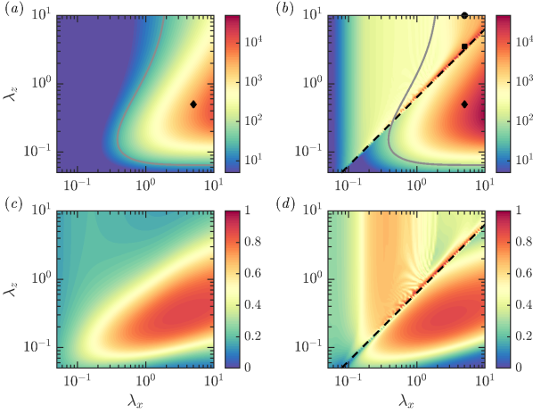
(a)

(b)

(c)

(d)

Figure 1: (a,b) The leading resolvent gain $\sigma_{1}$ as well as (c,d) the fraction of energy captured by the leading resolvent mode, computed as $LR=\sigma_{1}^{2}/(\sum_{i}\sigma_{i}^{2})$, are shown as a function of the streamwise and spanwise wavelengths ($\lambda_{x}$,$\lambda_{z}$) and a fixed phase speed $c=\overline{U}(y^{+}\approx 15)$. (a,c) An incompressible boundary layer with $Re_{\tau}=450$ and (b,d) a compressible boundary layer with $Ma=4$ and $Re_{\tau}=400$ over an adiabatic wall are considered. The black dashed line in (b,d) indicates the relative Mach number equal to unity. The grey contour line in (a) indicates $1/3$rd of the maximum energy in the incompressible case, and the same contour (computed from the incompressible case) also appears in (b) for comparison. The ($\blacklozenge$) in (a,b) and the ($\blacksquare$) and ($\bullet$) in (b) indicates the modes that are plotted in later figures.

Before looking at the different amplification mechanisms that are active in the compressible resolvent operator, in this section we first analyze the two types of modes that are amplified: (i) the subsonic modes that have equivalents in the incompressible flow and (ii) the supersonic modes that have no such equivalents in the incompressible flow (Bae et al., 2020b). For this purpose, in figure 1 we compare the responses obtained from a compressible boundary layer to that from an incompressible boundary layer. The leading resolvent norm $\sigma_{1}$ (6) obtained with respect to the streamwise and spanwise wavelengths $\lambda_{x}$ and $\lambda_{z}$, for a fixed value of $c=\overline{U}(y^{+}\approx 15)$, is shown for two cases: i) an incompressible flow at $Re_{\tau}=450$ in figure 1(1(a)) and ii) a compressible flow at $Re_{\tau}=400$ and $Ma=4$ in figure 1(1(b)). (It should be noted that, in figure 1, the full Chu norm (4) is shown for the compressible case, while the kinetic energy norm is plotted for the incompressible case, and that this difference does not have significant implications for the discussion in this section). We see that, in both the flows, there are regions of the wavenumber space that have high linear amplification (it should be noted that the color-scale is logarithmic). In figure 1(1(a)), the grey contour line indicates $1/3$rd of the maximum energy of the incompressible case. The same contour line, computed from the incompressible case, is also shown in figure 1(1(b)) for comparison. The black dashed line in figure 1(1(b)) indicates the region where the freestream relative Mach number is equal to unity $\overline{Ma}(\infty)=1$, where the relative Mach number is defined as

$$\overline{Ma}(y)=\frac{Ma(k_{x}\overline{U}(y)-\omega)}{\sqrt{(k_{x}^{2}+k_{z}^{2})\overline{\Theta}(y)}}.$$ (8)

The relative Mach number is the local Mach number of the mean flow relative to the phase-speed of the disturbance in the direction of the wave-number vector (Mack, 1984). Below the $\overline{Ma}(\infty)=1$ line, $\overline{Ma}(y)<1$ for all $y$. As was observed in Bae et al. (2020b) (and will also be explained here in §3.2) the supersonic modes from the resolvent operator do not exist in regions where $\overline{Ma}(y)<1$, and therefore these modes only appear above the black dashed line in figures 1(1(b)). It therefore means that only the subsonic resolvent modes are amplified in the region below the $\overline{Ma}(\infty)=1$ line in figure 1(1(b)). Comparing this region below the $\overline{Ma}(\infty)=1$ line to the incompressible flow in figure 1(1(a)), we see that similar regions of the wavenumber space are amplified in both flows. This similarity between the two flows is further discussed in §3.1.

Another metric that is used to analyze the resolvent operator is $LR=\sigma_{1}^{2}/(\sum_{i}\sigma_{i}^{2})$ (see §2.2), which is the fraction of energy that is captured by the first resolvent mode alone. In figure 1(1(c),1(d)) we plot $LR$ as a function of $(\lambda_{x},\lambda_{z})$. In the region of the $(\lambda_{x},\lambda_{z})$ space where $LR$ is high, the resolvent is low-rank and most of the energy from the resolvent resides in the first resolvent mode. The black dashed line in figure 1(1(d)) again indicates the $\overline{Ma}(\infty)=1$ line.

3.1 Subsonic modes

Let us first discuss the similarities between the compressible and the incompressible resolvent, and therefore consider the regions in figures 1(1(b), 1(d)) below the black dashed line, and compare it to the incompressible case in figures 1(1(a), 1(c)). In the incompressible flow in figure 1(1(a)), the most amplified structures are very long, i.e. with $\lambda_{x}\to\infty$. From figure 1(1(c)) we observe that a range of these energetic modes are also low-rank. When considering the compressible flow in figure 1(1(b)), the structures with $\lambda_{x}\to\infty$ are also amplified for this flow. The region bounded by the grey contour line is amplified for both the flows, further emphasising the similarities between the flows. The range of scales that show low-rank behaviour in figure 1(1(d)) is also very similar to those in the incompressible flow in figure 1(1(c)).

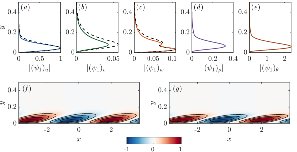
(a)

(b)

(c)

(d)

(e)

(f)

(g)

Figure 2: The leading resolvent response for the modes indicated by the diamonds ($\blacklozenge$) in figure 1(a,b) are shown. The mode corresponds to $\lambda_{x}=5$, $\lambda_{z}=0.5$ and $c=\overline{U}(y^{+}\approx 15)$. The wall-normal profile of the (a) streamwise, (b) wall-normal and (c) spanwise velocities are shown. The solid lines in (a-c) represents the mode from a compressible boundary layer with $Ma=4$ and $Re_{\tau}=400$ and the black dashed lines represents the mode from an incompressible boundary layer with $Re_{\tau}=450$. The profiles of (d) density and (e) temperature are also shown for the compressible case. The streamwise velocity $u$ in a $x-y$ plane for (f) the incompressible and (g) the compressible flow is also shown where red and blue indicates positive and negative velocity fluctuations, respectively, and the contour lines indicate $0.25-0.25-1.0$ of the maximum velocity.

To further analyze this similarity between the compressible and the incompressible resolvent we pick individual modes to compare. Let us consider the modes that are indicated with $({\scriptsize\blacklozenge})$ in figures 1(1(a)) and 1(1(b)), which corresponds to $\lambda_{x}=5$, $\lambda_{z}=0.5$ and $c=\overline{U}(y^{+}\approx 15)$. The three velocity components of the incompressible and compressible modes are shown in figures 2(2(a)-2(c)), with the solid lines representing the compressible mode and the black dashed line representing the incompressible mode. The streamwise $(\psi_{1})_{u}$, wall-normal $(\psi_{1})_{v}$ and spanwise $(\psi_{1})_{w}$ velocity components of the leading resolvent mode $\bm{\psi}_{1}$ obtained from (6) are shown in figures 2(2(a)), 2(2(b)) and 2(2(c)), respectively. For the case of the compressible flow the density $(\psi_{1})_{\rho}$ and temperature $(\psi_{1})_{\theta}$ components are also shown in figures 2(2(d)) and 2(2(e)), respectively. For both the incompressible as well as the compressible case, this mode is localized and resides within the boundary layer (note that the wall-normal direction in this figure is shown only till $0.5\delta$). The most important difference between the two flows is that, for the compressible flow, temperature and density are also amplified. These temperature and density profiles are also localized. As a further comparison, figure 2(2(g)) shows streamwise velocity $(\psi_{1})_{u}$ in a streamwise wall-normal ($x-y$) plane for the compressible flow which is compared to figure 2(2(f)) which shows $(\psi_{1})_{u}$ for the incompressible flow. We observe alternating streaks of high (red contours) and low (blue contours) momentum for both flows. Therefore in this region below the $\overline{Ma}(\infty)=1$ line in figure 1(1(b)), we observe that the compressible resolvent share similar trends to the incompressible resolvent. This similarity was discussed in Bae et al. (2020b), where they showed that when the compressible modes are scaled using the semi-local scaling of compressible flows (Trettel & Larsson, 2016), they collapse well onto the modes from the incompressible flow.

3.2 Supersonic modes

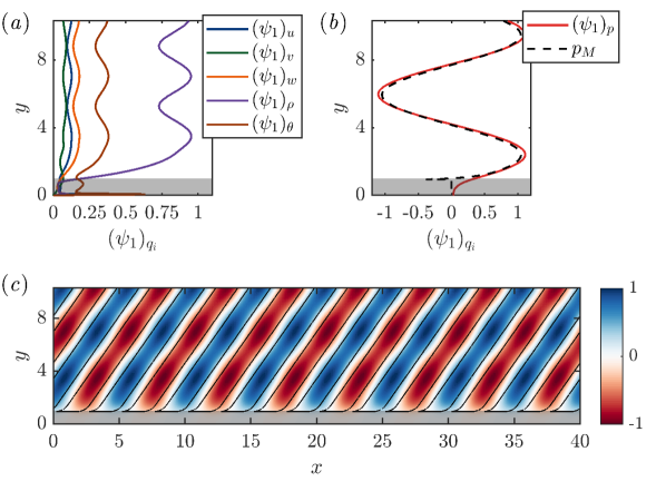
(a)

(b)

(c)

Figure 3: The leading resolvent response for the mode indicated by the ($\blacksquare$) in figure 1(b). The mode corresponds to $\lambda_{x}=5$, $\lambda_{z}=3.5$ and $c=\overline{U}(y^{+}\approx 15)$ for a compressible boundary layer with $Ma=4$ and $Re_{\tau}=400$ over an adiabatic wall. (a) The wall-normal profile of the streamwise (blue), wall-normal (green) and spanwise (orange) velocities, as well as the density (purple) and temperature (brown) are shown. (b) The wall-normal profile of the real part of the pressure from the resolvent mode (red) is compared with the pressure fluctuations from the inviscid Mach wave (black dashed) given by the equation (13). (c) The pressure fluctuations in a $x-y$ plane is also shown with red (positive) and blue (negative) contours showing the real part of the pressure fluctuation from the resolvent mode and the black contour lines indicating the pressure fluctuations from the inviscid Mach wave at $\pm 0.5$ of the maximum. The grey shaded regions indicate the boundary layer thickness.

So far we have concentrated on the subsonic modes that fall below the relative Mach equal to unity line in figure 1(1(b)). Let us now consider the region of the wavenumber space that fall above this line in figure 1(1(b)). The amplified modes in this region are the supersonic modes of the flow and in this section we will consider these modes and their connection to the relative Mach number defined in (8). For simplicity, let us here consider the inviscid equations for compressible boundary layers as studied in Mack (1984) and we will later analyze if the conclusions drawn are more generally applicable to the resolvent operator at finite Reynolds numbers. Unlike in Mack (1984), here we will keep the non-linear terms in the equations as an unknown forcing $\widehat{\bm{f}}$ as in (1), therefore giving us

$$\begin{split}i\overline{\rho}(k_{x}\overline{U}-\omega)\widehat{u}&=-\overline{\rho}\frac{d\overline{U}}{dy}\widehat{v}-\frac{1}{\gamma Ma^{2}}ik_{x}\widehat{p}+\widehat{f}_{u}\end{split}$$ (9a)

$$\begin{split}i\overline{\rho}(k_{x}\overline{U}-\omega)\widehat{v}&=-\frac{1}{\gamma Ma^{2}}\frac{\partial\widehat{p}}{\partial y}+\widehat{f}_{v}\end{split}$$ (9b)

$$\begin{split}i\overline{\rho}(k_{x}\overline{U}-\omega)\widehat{w}&=-\frac{1}{\gamma Ma^{2}}ik_{z}\widehat{p}+\widehat{f}_{w}\end{split}$$ (9c)

$$\begin{split}i\overline{\rho}(k_{x}\overline{U}-\omega)\widehat{\theta}&=\phantom{-}\overline{\Theta}\frac{\partial\overline{\rho}}{\partial y}\widehat{v}-(\gamma-1)\nabla\cdot\bm{u}+\widehat{f}_{\theta}\end{split}$$ (9d)

$$\begin{split}i\overline{\Theta}(k_{x}\overline{U}-\omega)\widehat{\rho}&=-\overline{\Theta}\frac{\partial\overline{\rho}}{\partial y}\widehat{v}-\nabla\cdot\bm{u}+\widehat{f}_{\rho}\end{split}$$ (9e)

$$\begin{split}\widehat{p}&=\overline{\Theta}\widehat{\rho}+\overline{\rho}\widehat{\theta}.\end{split}$$ (9f)

Here $\bm{u}=(u,v,w)$ and we have used $\overline{\rho}\overline{\Theta}=1$ to write $-\overline{\rho}\partial\overline{\Theta}/\partial y=\overline{\Theta}\partial\overline{\rho}/\partial y$. The equation for pressure is then rewritten using the equations for density and temperature as:

$$\begin{split}i(k_{x}\overline{U}-\omega)\widehat{p}&=-\gamma\nabla\cdot\bm{u}+\widehat{f}_{\theta}+\widehat{f}_{\rho}.\\ \end{split}$$ (10)

We note that, in addition to $\widehat{f}_{\rho}$ and $\widehat{f}_{\theta}$, the divergence of velocity $\nabla\cdot\bm{u}$ also amplifies pressure fluctuations, and this will become significant later when we consider the different mechanisms that can amplify the supersonic modes. Computing $\nabla\cdot\bm{u}$ from (9) and substituting into (10) we get

$$\begin{split}-(k_{x}\overline{U}-\omega)^{2}\widehat{p}&+\frac{\overline{\Theta}k^{2}}{Ma^{2}}\widehat{p}-\frac{1}{Ma^{2}}\frac{d\overline{\Theta}}{dy}\frac{\partial\widehat{p}}{\partial y}-\frac{\overline{\Theta}}{Ma^{2}}\frac{\partial^{2}\widehat{p}}{\partial y^{2}}=2i\gamma k_{x}\frac{dU}{dy}\widehat{v}\\ &-\gamma\frac{d\overline{\Theta}}{dy}\widehat{f}_{v}-\gamma\overline{\Theta}\nabla\cdot\widehat{\bm{f}}_{\bm{u}}+i(k_{x}\overline{U}-\omega)[\widehat{f}_{\theta}+\widehat{f}_{\rho}].\\ \end{split}$$ (11)

Here $k^{2}=k_{x}^{2}+k_{z}^{2}$ and $\widehat{\bm{f}}_{\bm{u}}=(\widehat{f}_{u},\widehat{f}_{v},\widehat{f}_{w})$. Substituting the equation of wall-normal velocity (9b) into (11) and using the definition of the relative Mach number $\overline{Ma}(y)=(Ma(k_{x}\overline{U}(y)-\omega))/(k\overline{\Theta}(y)^{1/2})$ from (8) we get:

$$\begin{split}-\frac{\partial^{2}\widehat{p}}{\partial y^{2}}&+\frac{d(\ln\overline{Ma}^{2})}{dy}\frac{\partial\widehat{p}}{\partial y}+k^{2}(1-\overline{Ma}^{2})\widehat{p}=\gamma Ma^{2}\frac{d(\ln\overline{Ma}^{2})}{dy}\widehat{f}_{v}\\ &+iMa^{2}\overline{\rho}(k_{x}\overline{U}-\omega)[\widehat{f}_{\theta}+\widehat{f}_{\rho}]-\gamma Ma^{2}\nabla\cdot\widehat{\bm{f}}_{\bm{u}}.\\ \end{split}$$ (12)

(Note that in (12) $Ma$ denotes the freestream Mach number and $\overline{Ma}$ denotes the relative Mach number defined in (8)). When $\overline{Ma}>1$ and we consider the freestream, the unforced equation for pressure (12) becomes a wave equation (the term $(d(\ln\overline{Ma})/dy)(\partial\widehat{p}/\partial y)$ vanishes in the freestream). In Mack (1984) this wave equation was solved to get the pressure fluctuations in the form of outgoing waves as

$$\widehat{p}=i\gamma\mbox{Ma}^{2}\left(\frac{k_{x}U-\omega}{k}\right)\exp{\left(-k\left(1-\overline{\mbox{Ma}}^{2}\right)^{1/2}y\right)}.$$ (13)

These are the Mach waves of the compressible boundary layer derived as solutions of the inviscid unforced equations. If we consider the discrete linear operator that governs the pressure (i.e. the left-hand-side (LHS) of (12)), these waves are singular vectors of the operator with singular value of $0$ (they also are eigenvectors with eigenvalue $0$). To consider the most amplified response to a forcing, we have to consider the singular vectors of the inverse of this linear operator, i.e. the inverse of the LHS of (12). In this case these waves in (13) will become infinitely amplified response directions (singular vectors with infinite amplification). Therefore, these Mach waves are also the most amplified responses to the forced equations in (12). Practically, these $0$ eigenvalues will make the LHS of (12) non-invertible and the addition of viscosity is necessary to regularise the linear operator and therefore obtain an inverse.

Now, to show that this mechanism of the Mach waves is captured by the compressible resolvent at the finite Reynolds numbers considered here, let us pick the mode marked by ($\blacksquare$) in figure 1(1(b)) that falls in the region above the $\overline{\mbox{Ma}}(\infty)=1$ line. The pressure $(\psi_{1})_{p}$ from the leading resolvent mode $\bm{\psi}_{1}$ is computed using the density $(\psi_{1})_{\rho}$ and the temperature $(\psi_{1})_{\theta}$ components as $(\psi_{1})_{p}=\overline{\Theta}(\psi_{1})_{\rho}+\overline{\rho}(\psi_{1})_{\theta}$. The real part of $(\psi_{1})_{p}$ is shown as the red solid line in figure 3(3(b)). In the same figure the real part of the Mach wave obtained using (13) is also shown in black (the amplitude and phase of the Mach wave is fixed to be the same as the resolvent mode at some arbitrary wall-height, here $y=5$). To compare the modes in physical space, $(\psi_{1})_{p}$ in a streamwise wall-normal ($x$-$y$) plane at a fixed spanwise location (here $z=0$) is also shown in figure 3(3(c)). The negative (blue) and positive (red) pressure fluctuations from the resolvent mode are shown, and the black line-contours represent the Mach wave from (13) (the contours represent $\pm 0.5$ of the maximum value). From these figures 3(3(b)) and 3(3(c)) we observe that, far from the wall, these resolvent modes are outgoing waves that radiate into the free-stream, and in the freestream they closely follow the behavior of the inviscid Mach wave. Figure 3(3(a)) shows the $u$, $v$, $w$, $\rho$ and $\theta$ components of the resolvent mode, and the oscillatory nature of the mode is evident in these components as well. This suggests that, within the freestream, the supersonic resolvent modes resemble the inviscid Mach waves in (13) and therefore the amplification mechanisms for both could be similar.

So far we have looked at an individual supersonic mode. Let us now consider a range of $(\lambda_{x},\lambda_{z})$ and therefore go back to figure 1(1(b)) which shows the leading resolvent gain $\sigma_{1}$ and figure 1(1(d)) which shows the low-rank behaviour of the modes through $LR$. Concentrating on the region above the black dashed line where the supersonic modes are present, we note two characteristics of these modes. First, the most amplified of these supersonic modes lie close to the $\overline{Ma}(\infty)=1$ line. Second, looking at the low-rank behaviour in figure 1(1(d)), we notice that the supersonic modes with large $\lambda_{x}$ that fall away from the $\overline{Ma}(\infty)=1$ line (top right corner of figure 1(1(d))) tend to have lower values of $LR$ in comparison to modes with smaller $\lambda_{x}$. This suggests the existence of more than one amplification mechanism that are active for these structures and is consistent with the fact that subsonic mechanisms are also active in this region, as indicated by the grey contour line in figure 1(1(b)) (indicating the region of the wavenumber space where the energy of the incompressible resolvent is greater than $1/3$rd of the maximum energy). This point is briefly revisited in §5.2 and §5.3.

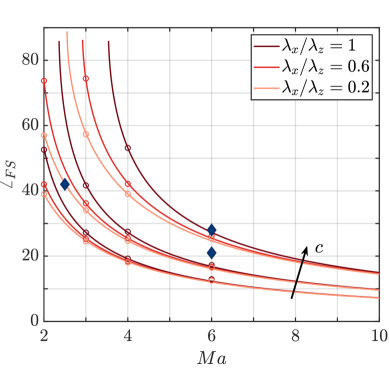
Figure 4: The inclination angle of the inviscid Mach waves given by the equation (13) is shown with respect to Mach number for a range of aspect ratios and phase speeds. Three different phase-speeds of $c=0.2,0.4\mbox{ and }0.6$ increasing in the direction of the arrow and three different values of aspect ratios $\lambda_{x}/\lambda_{z}=0.2,0.6\mbox{ and }1.0$ are shown. The open circles indicate the freestream inclination angle of the corresponding resolvent modes at that Mach number. The blue diamond markers (${\scriptsize\blacklozenge}$) indicate the average inclination angles of the Mach waves from DNS reported in the literature (Duan et al., 2014; Zhang et al., 2017). The DNS data at $Ma=6$ is for the case of cooled walls, and the two markers indicate two different ratios of $\Theta_{w}/\Theta_{ad}=0.25$ and $0.76$.

4 Some pertinent features of the subsonic and supersonic modes

This section will concentrate on some of the features of the subsonic and supersonic modes from the compressible resolvent operator. In S4.1 the freestream inclination angles of the supersonic modes are analyzed. Further §4.2 concentrates on the Helmholtz decomposition of the resolvent modes. And finally, §4.3 looks at the contribution of these resolvent modes to the boundary layer and the freestream, separately.

4.1 Inclination angle of the supersonic resolvent modes

To further compare the resolvent modes to the Mach waves as done in §3.2, let us look at the inclination angle of these modes. From (13) the freestream inclination angle of the Mach waves can be computed as:

$$\angle_{FS}=\tan^{-1}\left(\frac{-1j}{\sqrt{1+(\lambda_{x}/\lambda_{z})^{2}-\mbox{Ma}^{2}(1-c)^{2}}}\right)$$ (14)

At a fixed Mach number, we see that the inclination angle depends on the aspect ratio $\lambda_{x}/\lambda_{z}$ of the mode as well as its phase speed $c$. The solid lines in figure 4 shows $\angle_{FS}$ as a function of Mach number for a range of aspect ratios and phase-speeds. (From (14) we can get both upstream and downstream inclining waves, and only the downstream inclining waves can satisfy the boundary conditions (Mack, 1984) and are therefore shown in figure 4). The circles show the approximate inclination angle of the resolvent mode in the freestream (that is obtained by fitting an exponential to the freestream pressure obtained from the resolvent mode). The phase-speed increases in the direction of the arrow in figure 4, and for each phase-speed lighter coloured lines represent structures with smaller aspect ratios. The markers (${\scriptsize\blacklozenge}$) show the values of the average freestream inclination angles that are obtained from DNS (Duan et al., 2014; Zhang et al., 2017) from a $Ma=2.5$ flow over an adiabatic wall and a $Ma=6$ flow with two wall-cooling ratios of $\Theta_{w}/\Theta_{ad}=0.76\mbox{ and }0.25$ (indicated by the two markers at $Ma=6$).

We can make three different observations from figure 4. First, we note that the resolvent modes (the circles in figure 4) closely follow the inclination angles computed from the inviscid equations (14). This further demonstrates that, within the freestream, the supersonic resolvent modes can be understood reasonably well using the inviscid Mach waves. Second, we see from figure 4 that the phase speed of the mode significantly impacts its inclination angle with slower structures (i.e. lower values of $c$) having a smaller inclination angle. Aspect ratios on the other hand have a much less significant impact on the inclination angle, with larger aspect ratios having slightly higher inclination angles. This effect of the aspect ratio diminishes with increasing Mach numbers. Finally, we also observe that the inclination angles that are obtained from the model (both the full resolvent as well as the inviscid model) decrease with increasing Mach number, consistent with DNS (Duan et al., 2014). The average inclination angles obtained from DNS fall within the range of inclination angles that are observed from the model. However, the mechanism that is responsible for picking out the value of the predominant freestream inclination angle in the DNS is still not understood.

4.2 Helmholtz decomposition of the resolvent modes

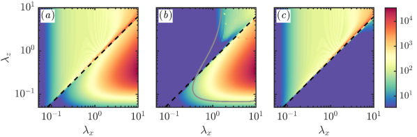
(a)

(b)

(c)

Figure 5: The kinetic energy of (a) the leading resolvent response $\bm{\psi}_{1}$ and of (b) the solenoidal and (c) the dilatational component of the velocity from $\bm{\psi}_{1}$ is shown as a function of the streamwise and spanwise wavelengths ($\lambda_{x}$, $\lambda_{z}$) and a fixed phase speed $c=\overline{U}(y^{+}\approx 15)$. The grey contour line in (b) is the same as that shown in figure 1(1(a)) and shows the kinetic energy for the incompressible case at $1/3$rd of the maximum.

One of the techniques that has been used to analyze compressible wall-bounded flows is the Helmholtz decomposition of the velocity. From DNS we know that the solenoidal component obtained from the Helmholtz decomposition of the velocity shows statistics similar to the incompressible case (Yu et al., 2019, 2020). In this section we will analyze the response of the resolvent using the Helmholtz decomposition.

The Helmholtz decomposition can be performed on any vector field, and here the vector field is the velocity field from the leading resolvent response mode $(\bm{\psi}_{1})_{\bm{u}}=((\psi_{1})_{u},(\psi_{1})_{v},(\psi_{1})_{w})$. This decomposition gives us two components of the vector: (i) a solenoidal component $(\bm{\psi}_{1})_{\bm{u}}^{s}$ which is divergence-free, i.e. $\nabla\cdot(\bm{\psi}_{1})_{\bm{u}}^{s}=0$ and (ii) a dilatational component $(\bm{\psi}_{1})_{\bm{u}}^{d}$ which is curl-free $\nabla\times(\bm{\psi}_{1})_{\bm{u}}^{d}=0$, such that $\bm{\psi}_{u}=(\bm{\psi}_{1})_{\bm{u}}^{s}+(\bm{\psi}_{1})_{\bm{u}}^{d}$. The Helmholtz decomposition is only unique up to the boundary conditions imposed, and we use $(\psi_{1})_{v}^{s}(y=0)=0$ and $(\psi_{1})_{u}^{d}(y=0)=(\psi_{1})_{w}^{d}(y=0)=0$ (Pirozzoli & Bernardini, 2011). Figure 5(5(b)) shows the kinetic energy of the solenoidal component and figure 5(5(c)) shows the kinetic energy of the dilatational component, which are compared to the full kinetic energy in figure 5(5(a)). The grey contour line in figure 5(5(b)) is the same as that shown in figure 1(1(a)) and shows kinetic energy for the incompressible case at $1/3$rd of the maximum, thereby indicating the region of the wavenumber space where the incompressible resolvent is reasonably amplified.

Let us first consider the region below the black dashed line, i.e. below the $\overline{Ma}(\infty)=1$ line, where only the subsonic modes are active. By comparing figures 5(5(b)) and 5(5(c)) to figure 5(5(a)) we see that the energy below this region resides almost entirely in the solenoidal component. This shows that the subsonic resolvent responses are divergence-free and therefore incompressible-like. This is consistent with observations from DNS (Yu et al., 2019). Now considering the region above the $\overline{Ma}(\infty)=1$ line where supersonic modes exist, from figure 5(5(c)) we notice that a lot of the energy in this region is dilatational. However, from figure 5(5(b)) we also see that there is a region of the wavenumber space which has a contribution from the solenoidal component as well. The grey contour indicates that this region is amplified in the incompressible flow as well. This suggests that these are modes where both the subsonic as well as supersonic mechanisms are active. This competition of different mechanisms also provides an explanation for the observed decrease in the low-rank behaviour of these modes that was noted in §3.2 (see figure 1(1(d))).

4.3 Energy of the resolvent modes within the boundary layer and the freestream

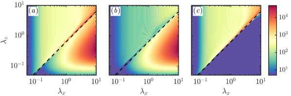
(a)

(b)

(c)

Figure 6: (a) The leading resolvent gain $\sigma_{1}$ is shown as a function of the streamwise and spanwise wavelengths $\lambda_{x}$ and $\lambda_{z}$ and for a fixed phase speed $c=\overline{U}(y^{+}\approx 15)$ (this is a reproduction of figure 1(1(b)) shown here for ease of comparison). The energy of the first resolvent mode that resides (b) within the boundary layer alone and (c) within the freestream alone are shown.

We now consider the wall-normal regions of the flow where the subsonic and supersonic modes are present. To study this, the energy of the first resolvent mode $\bm{\psi}_{1}$ can be split into two parts, the energy that resides within the boundary layer $\langle\bm{\psi}_{1},\bm{\psi}_{1}\rangle(y\leq 1)$ and the energy in the free-stream $\langle\bm{\psi}_{1},\bm{\psi}_{1}\rangle(y>1)$. Figure 6(6(b)) shows the energy within the boundary layer and figure 6(6(c)) the energy in the free-stream, which are compared to figure 6(6(a)) showing $\sigma_{1}$, i.e. the full energy in $\bm{\psi}_{1}$ (figure 6(6(a)) is a reproduction of figure 1(1(b)) shown here again for ease of comparison).

First considering the region below the black dashed line for the subsonic modes, we see that most of the energy in this region is captured in figure 6(6(b)). This implies that the subsonic modes largely reside within the boundary layer thickness. Looking at the supersonic modes above the black dashed line, we note that these modes are present both within the boundary layer from figure 6(6(b)) as well as in the freestream from figure 6(6(c)). More important though is the observation that only the supersonic modes contribute significantly to the freestream (in figure 6(6(c))), which is consistent with the observation that these modes are pressure fluctuations that radiate into the freestream. This observation is important for applications that seek to reduce the freestream noise radiated from a turbulent boundary layer (e.g. Laufer, 1964; Wagner Jr et al., 1970; Stainback, 1971; Pate, 1978; Schneider, 2001).

From §3 and §4 we can therefore conclude that the subsonic modes from the compressible resolvent operator are alternating streaks of high and low momentum that reside within the boundary layer and the velocities of these structures are divergence-free and therefore incompressible-like. The supersonic modes on the other hand are pressure fluctuations that radiate into the freestream and the most amplified of these modes have freestream relative Mach numbers close to unity. These modes are the sole contributors to the energy in the freestream of the flow. Within the freestream the supersonic modes follow the trends of the inviscid Mach waves well. The freestream inclination angles of the supersonic modes decrease with Mach number, consistent with DNS.

5 Mechanisms for the amplification of resolvent modes

In this section we analyze the forcing mechanisms that capture the two distinct flow features obtained from the resolvent operator for compressible boundary layers, (i) the subsonic features that is also present in the case of incompressible boundary layer flows, and (ii) the supersonic features that have no equivalent in the incompressible flow regime. Understanding these mechanisms will in §6 allow us to decompose the resolvent operator such that these two mechanisms are approximately isolated.

5.1 Forcing to the subsonic modes

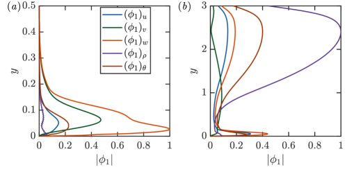
(a)

(b)

Figure 7: The leading forcing mode $\bm{\phi}_{1}$ for (a) a subsonic mode with $\lambda_{x}=5$, $\lambda_{z}=0.5$ and $c=\overline{U}(y^{+}\approx 15)$ (($\blacklozenge$) in figure 1(b)) and (b) a supersonic mode with $\lambda_{x}=5$, $\lambda_{z}=3.5$ and $c=\overline{U}(y^{+}\approx 15)$ (($\blacksquare$) in figure 1(b)) are shown. All five components of the forcing are shown, i.e. forcing to the streamwise (blue), wall-normal (green), spanwise (orange) momentum, continuity (purple) and temperature (brown) equations.

Let us first consider the subsonic modes, and concentrate on the leading forcing mode $\bm{\phi}_{1}$ obtained from the SVD of the resolvent operator (6). Figure 7(7(a)) shows the different components of $\bm{\phi}_{1}$ for the mode considered in figure 2 (the mode indicated by the ($\blacklozenge$) in figure 1(1(b))). The subscripts $u$, $v$, $w$, $\rho$ and $\theta$ represent the five different components of $\bm{\phi}_{1}$. We see that the spanwise and the wall-normal components of the forcing are the most significant. This is what we would expect from the lift-up mechanism that is responsible for the streak amplification in incompressible flows (e.g. Ellingsen & Palm, 1975; Jovanović & Bamieh, 2005; Illingworth, 2019), and therefore is consistent with the observations in literature that lift-up is also responsible for streak amplification in compressible flows (e.g. Hanifi & Henningson, 1998; Malik et al., 2008). Lift-up mechanism refers to the amplification of streaks of streamwise velocity, density and temperature that are forced by streamwise vortices ($v$ and $w$) (Ellingsen & Palm, 1975; Hanifi & Henningson, 1998). In compressible flows, the mean-shear $d\overline{U}/dy$ along with the mean-density gradient $d\overline{\rho}/dy$ (and therefore also the mean-temperature gradient $d\overline{\Theta}/dy$ which is related to $d\overline{\rho}/dy$ through $\overline{\rho}\overline{\Theta}=1$) drives this lift-up mechanism (Hanifi & Henningson, 1998).

In the case of the incompressible flow, it is also known that only the solenoidal component of the forcing has any active influence in amplifying resolvent modes (Rosenberg & McKeon, 2019; Morra et al., 2021). In this section we therefore ask if this property of incompressible flows carries over to the subsonic modes of the compressible flows. For this purpose we are required to perform a Helmholtz decomposition of the forcing to the momentum equations $\widehat{\bm{f}}_{\bm{u}}=(\widehat{f}_{u},\widehat{f}_{v},\widehat{f}_{w})$. The Helmholtz decomposition gives us two components of the vector: (i) a solenoidal component $\widehat{\bm{f}}_{\bm{u}}^{s}=(\widehat{f}^{s}_{u},\widehat{f}^{s}_{v},\widehat{f}^{s}_{w})$ which is divergence-free, i.e. $\nabla\cdot\widehat{\bm{f}}_{\bm{u}}^{s}=0$ and (ii) a dilatational component $\widehat{\bm{f}}_{\bm{u}}^{d}=(\widehat{f}^{d}_{u},\widehat{f}^{d}_{v},\widehat{f}^{d}_{w})$ which is curl-free $\nabla\times\widehat{\bm{f}}_{\bm{u}}^{d}=0$, such that $\widehat{\bm{f}}_{\bm{u}}=\widehat{\bm{f}}_{\bm{u}}^{s}+\widehat{\bm{f}}_{\bm{u}}^{d}$. The boundary conditions imposed are $\widehat{f}^{s}_{v}(y=0)=0$ and $\widehat{f}^{d}_{u}(y=0)=\widehat{f}^{d}_{w}(y=0)=0$ (Pirozzoli & Bernardini, 2011). It should be noted that, in the case of the incompressible flow, the dilatational component of the forcing is not zero, i.e. the divergence of the full forcing $\nabla\cdot\widehat{\bm{f}}_{\bm{u}}\neq 0$. However, only the solenoidal component of the forcing can directly excite a response in velocity (Rosenberg & McKeon, 2019; Morra et al., 2021).

To understand how this Helmholtz decomposition of the forcing impacts compressible boundary layers, let us, for the sake of simplicity, consider the inviscid equations (9) along with the Helmholtz decomposition of $\widehat{\bm{f}}_{\bm{u}}$. The curl-free condition of the dilatational component $\widehat{\bm{f}}_{\bm{u}}^{d}$ implies that it can be expressed in terms of the gradient of a scalar field $\widehat{\bm{f}}_{\bm{u}}^{d}=\nabla\zeta$. The $\zeta$ therefore will modify the pressure and only $\widehat{\bm{f}}_{\bm{u}}^{s}$ can force the velocity, giving

$$\begin{split}i\overline{\rho}(k_{x}\overline{U}-\omega)\widehat{u}_{i}&=-\overline{\rho}\frac{\partial\overline{U}}{\partial y}\widehat{v}\mbox{ }\widehat{\bm{i}}-\frac{1}{\gamma Ma^{2}}\frac{\partial(\widehat{p}+\widehat{\zeta})}{\partial x_{i}}+\widehat{f}^{s}_{u_{i}}.\\ \end{split}$$ (15)

The decomposition as in (15) is the same as seen for incompressible flows. Furthermore, from the continuity (9d) and energy (9e) equations we also see that $\widehat{f}_{\rho}$ and $\widehat{f}_{\theta}$ cannot directly influence the velocity fields. Only $\widehat{\bm{f}}_{\bm{u}}^{s}$ can force $v$ and $w$ and therefore generate a streamwise vortex required for lift-up. This streamwise vortex will in turn then amplify the streaks of $u$, $\rho$ and $\theta$ (using the mean shear $d\overline{U}/dy$ and the mean density gradient $d\overline{\rho}/dy$) (Hanifi & Henningson, 1998). It is therefore reasonable to expect that the solenoidal component of the forcing, on its own, will capture the subsonic modes of the compressible flow well.

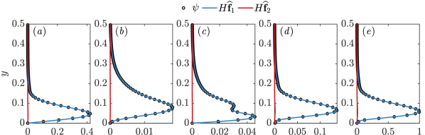
(a)

(b)

(c)

(d)

(e)

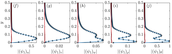
(f)

(g)

(h)

(i)

(j)

Figure 8: The response of the resolvent operator to the full leading resolvent forcing mode $\bm{\phi}_{1}$ (black) as well as the response to the two components of the forcing $\widehat{\bm{f}}_{1}$ (blue) and $\widehat{\bm{f}}_{2}$ (red) are shown. Subsonic modes with $(\lambda_{x},\lambda_{z},c)=(5,0.5,\overline{U}(y^{+}\approx 15))$ for two compressible boundary layers are shown: (a-e) $Ma=4$, $Re_{\tau}=400$ over an adiabatic wall (the mode indicated by the ($\blacklozenge$) in figure 1(1(b))) and (f-j) $Ma=6$, $Re_{\tau}=450$ with $\Theta_{w}/\Theta_{ad}=0.25$. The (a,f) streamwise, (b,g) wall-normal and (c,h) spanwise velocities as well as the (d,i) density and (e,j) temperature are shown.

To see if these arguments made using the inviscid equations have any bearing to the full compressible resolvent operator at a finite Reynolds number, we consider the subsonic mode that we previously discussed in figure 2 with $\lambda_{x}=5$, $\lambda_{z}=0.5$ and $c=\overline{U}(y^{+}\approx 15)$ for a $Re_{\tau}=400$ boundary layer with $Ma=4$ and adiabatic walls. In figures 8(8(a)-8(e)) the five components of the leading resolvent response mode $\bm{\psi}_{1}$ are shown. To show that this analysis is more generally valid, in figures 8(8(f)-8(j)) we also consider a $Re_{\tau}=450$ boundary layer flow with a higher Mach number of $Ma=6$, over a cooled wall with wall-cooling ratio $\Theta_{w}/\Theta_{ad}=0.25$. The five components of the full response is shown in black with the panels from left to right indicating the components $(\psi_{1})_{u}$, $(\psi_{1})_{v}$, $(\psi_{1})_{w}$, $(\psi_{1})_{\rho}$ and $(\psi_{1})_{\theta}$, respectively. In blue the response of the resolvent operator to the solenoidal component of the forcing alone, i.e. where the forcing to the resolvent operator is taken to be $\widehat{\bm{f}}_{1}=(\widehat{f}^{s}_{u},\widehat{f}^{s}_{v},\widehat{f}^{s}_{w},0,0)$, is shown. And in red is shown the response to the remaining components of the forcing, i.e. $\widehat{\bm{f}}_{2}=(\widehat{f}^{d}_{u},\widehat{f}^{d}_{v},\widehat{f}^{d}_{w},\widehat{f}_{\rho},\widehat{f}_{\theta})$. As anticipated, all three components of velocity, as well as density and temperature of the response are entirely captured by $\widehat{\bm{f}}_{\bm{u}}^{s}$. It can also be shown (not demonstrated here for the sake of brevity) that the response to $\widehat{\bm{f}}_{\bm{u}}^{s}$ is captured by the spanwise and wall-normal components of $\widehat{\bm{f}}_{\bm{u}}^{s}$, consistent with the mechanism being that of lift-up. From the red lines in figures 8, we see that the other components of the forcing $\widehat{\bm{f}}_{\bm{u}}^{d}$, $\widehat{f}_{\rho}$ and $\widehat{f}_{\theta}$ have negligible influence on the subsonic modes. Additionally, from figures 8(8(f)-8(j)), we see that wall-cooling does not impact any of these trends. (The forcing $\widehat{\bm{f}}_{1}$ and $\widehat{\bm{f}}_{2}$ are defined such that the full leading forcing mode of the resolvent $\bm{\phi}_{1}=\widehat{\bm{f}}_{1}+\widehat{\bm{f}}_{2}$. The definitions of $\widehat{\bm{f}}_{1}$ and $\widehat{\bm{f}}_{2}$ will be encountered again in the following sections).

5.2 Forcing to the supersonic modes

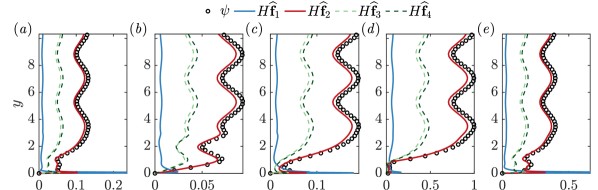
(a)

(b)

(c)

(d)

(e)

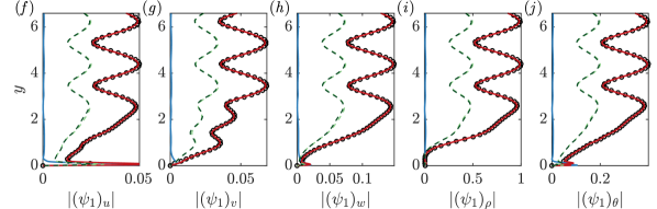
(f)

(g)

(h)

(i)

(j)

Figure 9: The response of the resolvent operator to the full leading resolvent forcing mode $\bm{\phi}_{1}$ (black) as well as the response to the two components of the forcing $\widehat{\bm{f}}_{1}$ (blue) and $\widehat{\bm{f}}_{2}$ (red) are shown. Two compressible boundary layers are considered: (a-e) $Ma=4$, $Re_{\tau}=400$ over an adiabatic wall and (f-j) $Ma=6$, $Re_{\tau}=450$ with $\Theta_{w}/\Theta_{ad}=0.25$. Modes that fall close to the relative Mach equal to unity lines are shown: mode $(\lambda_{x},\lambda_{z},c)=(5,3.5,\overline{U}(y^{+}\approx 15))$ for the $Ma=4$ case (the mode indicated by the ($\blacksquare$) in figure 1(1(b))) and mode $(\lambda_{x},\lambda_{z},c)=(5,1.6,\overline{U}(y^{+}\approx 15))$ for the $Ma=6$ case. The (a,f) streamwise, (b,g) wall-normal and (c,h) spanwise velocities as well as the (d,i) density and (e,j) temperature are shown.

We now consider the supersonic modes, and the leading resolvent forcing mode $\bm{\phi}_{1}$ (6) for these modes. Figure 7(7(b)) shows the five different components of the forcing for the supersonic mode that was considered in figure 3 (the mode indicated by the ($\blacksquare$) in figure 1(1(b))). We note that the forcing to the continuity and temperature equations are now important. As investigated for the subsonic modes, to get a more complete picture of the forcing mechanisms, we consider the Helmholtz decomposition of the forcing to the momentum equations $\widehat{\bm{f}}_{\bm{u}}$. For simplicity, let us again consider the inviscid equations, and here specifically the inviscid pressure equation (12) in terms of the solenoidal $\widehat{\bm{f}}_{\bm{u}}^{s}$ and the dilatational $\widehat{\bm{f}}_{\bm{u}}^{d}$ components of $\widehat{\bm{f}}_{\bm{u}}$,

$$\begin{split}-\frac{\partial^{2}\widehat{p}}{\partial y^{2}}+\frac{d(\ln\overline{Ma}^{2})}{dy}&\frac{\partial\widehat{p}}{\partial y}+k^{2}(1-\overline{Ma}^{2})\widehat{p}=\gamma Ma^{2}\frac{d(\ln\overline{Ma}^{2})}{dy}\left[\widehat{f}^{s}_{v}+\widehat{f}^{d}_{v}\right]\\ &+iMa^{2}\overline{\rho}(k_{x}\overline{U}-\omega)[\widehat{f}_{\theta}+\widehat{f}_{\rho}]-\gamma Ma^{2}\nabla\cdot\widehat{\bm{f}}_{\bm{u}}^{d}.\\ \end{split}$$ (16)

From (16) we see that $d_{\rho}$ and $d_{\theta}$ now have a direct role in exciting these Mach waves. Another component that has a contribution is the dilatational component of the forcing to the momentum equations through $\nabla\cdot\widehat{\bm{f}}_{\bm{u}}^{d}$. Let us first concentrate on the impact of these two components, and we will consider the effect of the solenoidal component of the forcing in (16) later in this section.

In figures 9(9(a)-9(e)) we look at the supersonic mode that was previously studied in figure 3 for a $Re\approx 400$ boundary layer with $Ma=4$ and an adiabatic wall. For the phase-speed $c\approx U(y^{+}=15)$, the mode corresponding to $\lambda_{x}=5$ and $\lambda_{z}=3.5$ is chosen, such that it falls very close to the relative Mach equal to unity line (as seen by the the ($\blacksquare$) that indicates this mode in figure 1(1(b))). This mode therefore is one of the most amplified supersonic modes for the chosen streamwise wavelength and phase-speed. To access the more general applicability of the discussions here, in figures 9(9(f)-9(j)), we also look at a supersonic mode for a $Re_{\tau}=450$ boundary layer flow at a higher Mach number of $Ma=6$ and over a cooled wall with $\Theta_{w}/\Theta_{ad}=0.25$. Here again we choose a mode that falls close to the relative Mach equal to unity line which for $c\approx U(y^{+}=15)$ and $\lambda_{x}=5$ corresponds to $\lambda_{z}=1.6$. The five components of the full response is shown in black with the panels from left to right indicating the components $(\psi_{1})_{u}$, $(\psi_{1})_{v}$, $(\psi_{1})_{w}$, $(\psi_{1})_{\rho}$ and $(\psi_{1})_{\theta}$, respectively. In red is the response of the resolvent to the dilatational forcing $\widehat{\bm{f}}_{\bm{u}}^{d}$ as well as $\widehat{f}_{\rho}$ and $\widehat{f}_{\theta}$, i.e. the forcing to the resolvent is $\widehat{\bm{f}}_{2}=(\widehat{f}^{d}_{u},\widehat{f}^{d}_{v},\widehat{f}^{d}_{w},\widehat{f}_{\rho},\widehat{f}_{\theta})$. And in blue is the response to the remaining components of the forcing, i.e. the solenoidal component of the forcing $\widehat{\bm{f}}_{1}=(\widehat{f}^{s}_{u},\widehat{f}^{s}_{v},\widehat{f}^{s}_{w},0,0)$. (The forcing $\widehat{\bm{f}}_{1}$ and $\widehat{\bm{f}}_{2}$ are the same as that defined in the previous section §5.1, and is such that the full leading forcing mode of the resolvent $\bm{\phi}_{1}=\widehat{\bm{f}}_{1}+\widehat{\bm{f}}_{2}$).

From figure 9, we see that $\widehat{\bm{f}}_{2}$ is responsible for capturing the majority of the energy in the modes considered. The component $\widehat{\bm{f}}_{1}$ plays an insignificant role for these modes. Further, the contribution of the dilatational component $\widehat{\bm{f}}_{3}=(\widehat{f}^{d}_{u},\widehat{f}^{d}_{v},\widehat{f}^{d}_{w},0,0)$ alone to the response (denoted by $H\widehat{\bm{f}}_{3}$ in figure 9) and of the density and temperature forcing $\widehat{\bm{f}}_{4}=(0,0,0,\widehat{f}_{\rho},\widehat{f}_{\theta})$ alone (denoted by $H\widehat{\bm{f}}_{4}$ in figure 9) are shown in two separate shades of green. Notably, for this particular mode at least, both $\widehat{\bm{f}}_{\bm{u}}^{d}$, as well as $\widehat{f}_{\rho}$ and $\widehat{f}_{\theta}$ contribute almost equally. From figures 9(9(f)-9(j)) we see that wall cooling does not affect these trends. It should be noted that the role of the forcing to the momentum equation $\widehat{\bm{f}}_{\bm{u}}$ in exciting the Mach waves is through the generation of a divergence of the velocity $\nabla\cdot\bm{u}$ which then forces the pressure equations (see (10)). For this mode therefore, the dilatational component of the forcing to the momentum equations generate a velocity with $\nabla\cdot\bm{u}\neq 0$ which then excites the supersonic modes.

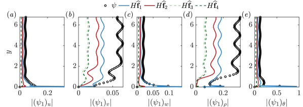
(a)

(b)

(c)

(d)

(e)

Figure 10: The response of the resolvent operator to the full leading resolvent forcing mode $\bm{\phi}_{1}$ (black) as well as the response to the two components of the forcing $\widehat{\bm{f}}_{1}$ (blue) and $\widehat{\bm{f}}_{2}$ (red) are shown. A supersonic mode with $(\lambda_{x},\lambda_{z},c)=(5,10,\overline{U}(y^{+}\approx 15))$ for a compressible boundary layer over an adiabatic wall with $Ma=4$, $Re_{\tau}=400$ is considered (the mode indicated by the ($\bullet$) in figure 1(1(b))). The (a) streamwise, (b) wall-normal and (c) spanwise velocities as well as the (d) density and (e) temperature are shown.

Let us now consider the impact of the solenoidal component of the forcing in (16). In figure 10 we consider a mode where the effect of the solenoidal forcing can be observed more readily. Here $\lambda_{x}=5$, $\lambda_{z}=10$ and $c=\overline{U}(y^{+}\approx 15)$. For this mode we find that the contribution of $\widehat{\bm{f}}_{1}$, and therefore the solenoidal component of the forcing, is significant (blue lines in figure 10). Firstly, there is a near-wall component captured by the solenoidal forcing. This again suggests that, along with the amplification of the Mach waves, the subsonic mechanisms are also active for these modes (see §3.2 and §4.2). Secondly, the response to the solenoidal forcing is not constrained to be divergence-free, and can therefore excite the Mach waves as seen in figure 10. However, in choosing the mode considered in figure 10 we picked a relatively less amplified supersonic mode, i.e. a mode that falls away from the relative Mach equal to unity line as shown by the ($\bullet$) in figure 1(1(b)). Therefore, it could be possible that the solenoidal component of the forcing becomes important only for the less amplified supersonic modes. We will see if this argument is justified by considering such a decomposition of the forcing over a range if $(k_{x},k_{z},c)$ and for different flow regimes in §6.

5.3 Suboptimal modes

So far we have only considered the leading resolvent mode. In this section we briefly consider the effect that the different forcing components have on the suboptimal modes as well. In figure 11 the first 10 resolvent modes, i.e. those corresponding to $\sigma_{1}-\sigma_{10}$ (6) are shown. Two $(k_{x},k_{z})$ pairs are considered: (i) the subsonic mode indicated by ($\blacklozenge$) in figure 1(1(b)) is shown in figure 11(11(a)) and (ii) the supersonic mode indicated by ($\blacksquare$) in figure 1(1(b)) is shown in figure 11(11(b)). The Chu norm of the response to the full resolvent forcing mode $\bm{\phi}_{i}$ is depicted in black, while the response to the solenoidal component of the forcing $\widehat{\bm{f}}_{1}=(\widehat{f}^{s}_{u},\widehat{f}^{s}_{v},\widehat{f}^{s}_{w},0,0)$ is shown in blue and the response to the remaining components $\widehat{\bm{f}}_{2}=(\widehat{f}^{d}_{u},\widehat{f}^{d}_{v},\widehat{f}^{d}_{w},\widehat{f}_{\rho},\widehat{f}_{\theta})$ is shown in red. (The energy of the full response is equal to the sum of the energies of the response to $\widehat{\bm{f}}_{1}$, the response to $\widehat{\bm{f}}_{2}$ and twice the cross correlations between these two components. While the energies of the responses to $\widehat{\bm{f}}_{1}$ and $\widehat{\bm{f}}_{2}$ are positive, the cross-correlations can be negative. Hence, for certain modes, such as for the $N=4$ mode in the supersonic case, the energy of the individual components $\widehat{\bm{f}}_{1}$ or $\widehat{\bm{f}}_{2}$ is higher than the full response in black).

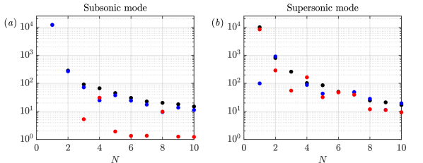
(a)

(b)

Figure 11: The Chu norm of the response of the resolvent operator to the full resolvent forcing mode $\bm{\phi}_{i}$ (black) as well as the two components of the forcing $\widehat{\bm{f}}_{1}$ (blue) and $\widehat{\bm{f}}_{2}$ (red) are shown for the first 10 resolvent modes. (a) The subsonic mode considered in figure 8 and (b) the supersonic mode considered in figure 9 are shown.

Considering the response of the subsonic mode in figure 11(11(a)), we find that the first three modes are captured by the solenoidal component of the forcing (the red dotes are not visible for $N=1,2$ since they fall below range of $y-$axis shown in the figure). When considering the supersonic mode, we find that the gap between the first and the second modes is reduced, and the second resolvent mode is captured by the solenoidal component of the forcing. This suggests, as seen before, two mechanisms being present in the amplification of the mode: the subsonic and the supersonic mechanisms. The supersonic mechanisms are most active for the mode considered here, and therefore appears as the first resolvent mode. For the current work, we leave the discussion of the suboptimal modes at this point, while noting that this topic requires further investigation, especially when constructing a reduced order model of the flow by computing the projections of the true forcing (from DNS) onto the resolvent forcing modes.

6 Decomposition of the forcing to the resolvent operator

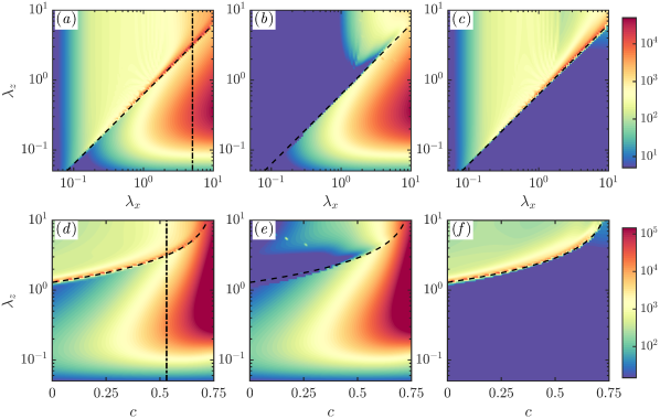
(a)

(b)

(c)

(d)

(e)

(f)

Figure 12: The Chu norm of the response of the resolvent operator to (a,d) the full leading resolvent forcing mode $\bm{\phi}_{1}$ as well as the two components of the forcing (b,e) $\widehat{\bm{f}}_{1}$ and (c,f) $\widehat{\bm{f}}_{2}$ are shown in two ways: (a-c) as a function of the streamwise and spanwise wavelengths $(\lambda_{x},\lambda_{z})$ at a fixed phase-speed $c=\overline{U}(y^{+}\approx 15)$ and (d-f) as a function of phase-speeds and spanwise wavelengths (c,$\lambda_{z}$) at a fixed streamwise wavelengths $\lambda_{x}=5$. The vertical dashed-dot line in (a) indicates $\lambda_{x}=5$ in (d) indicates $c=\overline{U}(y^{+}\approx 15)$. The dashed contour lines indicate the relative Mach equal to unity.

We have so far seen that the solenoidal component of the forcing to the momentum equations $\widehat{\bm{f}}_{1}=(\widehat{f}^{s}_{u},\widehat{f}^{s}_{v},\widehat{f}^{s}_{w},0,0)$ capture the subsonic modes of the compressible boundary layer and the dilatational component along with the forcing to the continuity and temperature equations $\widehat{\bm{f}}_{2}=(\widehat{f}^{d}_{u},\widehat{f}^{d}_{v},\widehat{f}^{d}_{w},\widehat{f}_{\rho},\widehat{f}_{\theta})$, while does not capture the full energy of the supersonic modes, still captures a majority of the energy of these modes. The aim in this section is to see if these arguments that were made by considering individual modes, is more generally applicable over a range of $(k_{x},k_{z},c)$ as well as for different flow regimes.

In figure 12 the responses of the resolvent to $\widehat{\bm{f}}_{1}$ and $\widehat{\bm{f}}_{2}$ are compared to the full resolvent response for the case of the turbulent boundary layer at $Ma=4$ and $Re_{\tau}=400$. The full response is shown in the first column of the figure (figures 12(12(a),12(d))) and the responses to $\widehat{\bm{f}}_{1}$ in the second (figures 12(12(b),12(e))) and to $\widehat{\bm{f}}_{2}$ in the third (figures 12(12(c),12(f))) columns. The first row of the figure (figures 12(12(a)-12(c))) shows the responses as a function of ($\lambda_{x}$,$\lambda_{z}$) at a fixed value of $c=U(y^{+}\approx 15)$. To consider a range of $c$, the second row of the figure (figures 12(12(d)-12(f))) shows the responses as a function of phase-speeds $c$ and $\lambda_{z}$, at a fixed value of $\lambda_{x}=5$. (The values of $c$ in figures 12(12(d)-12(f)) are taken only till $0.75$, since the amplification of the subsonic streaks with $c>0.75$ is very high making it hard to depict the amplification of these modes along with the amplification of the supersonic modes on the same figure). The black dashed lines in the figures (or curves in the case of figures 12(12(d)-12(f))) indicates relative Mach equal to unity. It is important to note that the colour-scale in figure 12 is logarithmic.

From figures 12(12(b),12(e)) we observe that $\widehat{\bm{f}}_{1}$ captures the responses in the subsonic modes, i.e. the responses in the region below the relative Mach equal to unity line. On the other hand, figures 12(12(c),12(f)) shows that $\widehat{\bm{f}}_{2}$ captures the majority of the response in the supersonic modes, i.e. the responses in the region above the relative Mach equal to unity line. This is especially true when considering the most amplified supersonic modes that fall close to the relative Mach equal to unity line. The contribution of $\widehat{\bm{f}}_{1}$ in the supersonic region is not zero as seen from figures 12(12(b),12(e)). However, as noted in §5.2, this response to $\widehat{\bm{f}}_{1}$ in the supersonic region becomes significant only for the less amplified supersonic modes that fall away from the relative Mach equal to unity line or for modes with large $c$ and $\lambda_{z}$ (figure 12(12(e))) where subsonic mechanisms are very energetic (see also §4.2). As a result, within the majority of the wavenumber space that falls above the relative Mach equal to unity line, the contribution of $\widehat{\bm{f}}_{2}$ is orders of magnitude higher than the contribution to $\widehat{\bm{f}}_{1}$ (given that the color-scale is logarithmic). Therefore, for this turbulent boundary layer flow at $Ma=4$, $Re_{\tau}=400$, the decomposition of the forcing into the two components $\widehat{\bm{f}}_{1}$ and $\widehat{\bm{f}}_{2}$ does approximately isolate the subsonic and supersonic modes.

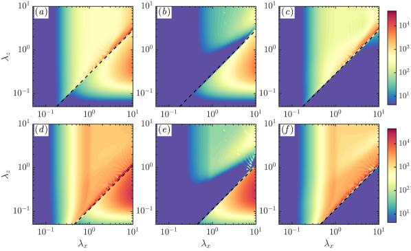
(a)

(b)

(c)

(d)

(e)

(f)

Figure 13: The Chu norm of the response of the resolvent operator to (a,d) the full leading resolvent forcing mode $\bm{\phi}_{1}$ as well as the two components of the forcing (b,e) $\widehat{\bm{f}}_{1}$ and (c,f) $\widehat{\bm{f}}_{2}$ are shown as a function of the streamwise ($\lambda_{x}$) and spanwise ($\lambda_{z}$) wavelengths for a fixed value of phase speed $c=\overline{U}(y^{+}\approx 15)$. Turbulent boundary layers with (a-c) $Ma=6$, $Re_{\tau}=450$ and $\Theta_{w}/\Theta_{ad}=0.25$ and (d-f) $Ma=14$, $Re_{\tau}=650$ and $\Theta_{w}/\Theta_{ad}=0.18$ are considered. The dashed lines indicate the relative Mach equal to unity.

What remains is to show that the decomposition works for a wider range of flow regimes. In figure 13 we therefore consider the responses as a function of ($\lambda_{x}$,$\lambda_{z}$) for a fixed $c=U(y^{+}\approx 15)$ for two flows: in the first row of figure 13 a $Ma=6$, $Re_{\tau}=450$ turbulent boundary layer over a cooled wall with wall-cooling ratio $\Theta_{w}/\Theta_{ad}=0.25$ is shown, and in the second row of figure 13 a higher Mach number $Ma=14$, $Re_{\tau}=650$ turbulent boundary layer with $\Theta_{w}/\Theta_{ad}=0.18$ is shown. For both cases the first column represents the response to the full forcing, the second column the response to $\widehat{\bm{f}}_{1}$ and the third column shows the response to $\widehat{\bm{f}}_{2}$. In general we notice that the decomposition is also valid for these higher Mach number flows as well with $\widehat{\bm{f}}_{1}$ capturing the response in the subsonic regions and $\widehat{\bm{f}}_{2}$ capturing a majority of the response in the supersonic regions. The relatively small contribution of $\widehat{\bm{f}}_{1}$ in the supersonic region is also evident for these cases. Importantly, both the cases considered in figure 13 are over cooled walls, and therefore the discussion regarding the decomposition of the forcing is valid for the case of flows over cooled walls as well.

6.1 A discussion on the decomposition of the forcing

At this point, it is important to note that, to understand the implications of this decomposition of the forcing for the real flow, we need to consider the projection of the non-linear terms computed from DNS or experimental data onto the resolvent forcing modes, i.e. compute the value of $\chi_{i}$ in (7). For instance, the analysis here, which does not consider any preferred wall-normal shape to the forcing to the resolvent, suggests that the solenoidal component has a less significant role in exciting the supersonic modes. However, this component of the forcing tends to be active close to the wall and this is the region where turbulent eddies are the most energetic, and can therefore project more easily onto the forcing. This could hypothetically mean that the projection of the non-linear terms onto solenoidal component of the forcing is significant, and therefore that this component can contribute to the amplification of the supersonic modes. Therefore, computing the projection of the true forcing from DNS or experiments onto the resolvent forcing modes is required to have a final say on the relative importance of the identified mechanisms on the amplification of the supersonic modes. This though is beyond the scope of the current manuscript, and is left as a question to be pursued for future work. Another important question for the future is to see if this decomposition can be used to approximately model the compressible part of the flow when DNS data is only available from the incompressible flow at a matched Reynolds number. Answering this question will have implications for the modelling of compressible flows.

7 Conclusions

We studied compressible boundary layers using the linearized Navier-Stokes equations. The non-linear terms of the momentum ($\widehat{\bm{f}}_{\bm{u}}$), continuity ($\widehat{f}_{\rho}$) and temperature ($\widehat{f}_{\theta}$) equations were treated as a forcing to the linearized equations. The resolvent analysis technique was used to analyze the system. In this technique a singular value decomposition is performed on the linear operator which gives the most sensitive forcing direction of the operator (right singular vectors), the corresponding most amplified response direction (left singular vectors) and also the amplification of this response (singular values). Consistent with the observations of Bae et al. (2020b), two types of modes are amplified by the compressible resolvent operator: (i) the subsonic modes that have an equivalent in the incompressible flow and (ii) the supersonic modes that do not have an equivalent in the incompressible flow (figure 1).

The subsonic modes are alternating streaks of high and low momentum that are localized within the boundary layer, similar to the modes found in the incompressible regime (figures 2 and figure 6). The velocities of these structures are divergence-free (figure 5). The spanwise and wall-normal components of the forcing are identified as the most sensitive (figure 7(7(a))), consistent with the amplification mechanism being that of lift-up. Only the solenoidal component of the forcing to the momentum equations $\widehat{\bm{f}}_{\bm{u}}^{s}$ can amplify these modes (figure 12). All the other components of forcing, that includes the dilatational component of the forcing to the momentum equations $\widehat{\bm{f}}_{\bm{u}}^{d}$, as well as the forcing to the density $\widehat{f}_{\rho}$ and temperature $\widehat{f}_{\theta}$ equations, play a negligible role in amplifying the subsonic modes. This is consistent with what has been previously observed in the incompressible regime (Rosenberg & McKeon, 2019; Morra et al., 2021), and it is interesting to note that a similar mechanism is active in the compressible regime as well.

Now considering the supersonic modes, we found that these resolvent modes are pressure fluctuations that radiate into the free-stream of the boundary layer (figures 3), and only these modes have any contribution towards the energy in the freestream of the flow (figures 6). Importantly, within the freestream, these resolvent modes closely follow the trends of the inviscid Mach waves (Mack, 1984). The freestream inclination angle of these structures that is predicted by the model decrease with Mach number (figure 4), consistent with DNS. We then identified the most sensitive forcing direction for these modes by analyzing the inviscid equations for pressure fluctuations. The dilatational component of the forcing to the momentum equations $\widehat{\bm{f}}_{\bm{u}}^{d}$, along with the forcing to the continuity $\widehat{f}_{\rho}$ and temperature $\widehat{f}_{\theta}$ equations capture a majority of the energy in these modes (figure 12). Additionally, there is also an effect from the solenoidal component of the forcing, which however has a significantly lower contribution to the resolvent response when considering unit amplitude broadband forcing. However, in future work, to understand the relative importance of these different mechanisms in exciting the Mach waves in the real flow, there is a need to compute the projection of the true non-linear terms (from DNS or experiments) onto the resolvent forcing modes.

Based on these observations regarding the subsonic and supersonic resolvent modes, a decomposition of the forcing to the resolvent operator was proposed which approximately isolates the subsonic and the supersonic modes. For the case of the subsonic modes, the solenoidal component of the forcing $\widehat{\bm{f}}_{\bm{u}}^{s}$ captures all of the amplification of these modes. In the case of the supersonic modes, the dilatational component, along with the forcing to the temperature and density equations (i.e. $\widehat{\bm{f}}_{\bm{u}}^{d}$, $\widehat{f}_{\rho}$ and $\widehat{f}_{\theta}$), capture the majority of the energy of these modes. We found that this decomposition isolates the subsonic and supersonic modes reasonably well for turbulent boundary layers both over adiabatic as well as cooled walls for a range of Mach numbers (figure 13).

8 Acknowledgements

We acknowledge support from the Air Force Office of Scientific Research grant FA9550-20-1-0173. We would also like to thank Prof. Anthony Leonard and Mr. Greg Stroot for helpful discussions regarding this work.

Appendix A Grid convergence

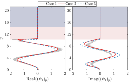
(a)

(b)

Figure 14: The real and imaginary parts of the pressure from the leading resolvent response for a supersonic mode. The mode corresponds to $\lambda_{x}=5$, $\lambda_{z}=3.5$ and $c=\overline{U}(y^{+}\approx 15)$ for a compressible boundary layer over an adiabatic wall with $Ma=4$ and $Re_{\tau}=400$ (the mode indicated by the ($\blacksquare$) in figure 1(b)). The modes obtained using three different grids are shown: (i) Case 1: the grid used in this work but without a damping layer, (ii) Case 2: the grid used in this work with $N=401$, $y_{max}=4\delta$ and $y_{max}=3l$ in the subsonic and supersonic regions, respectively and (iii) Case 3: with $N=601$, $y_{max}=5\delta$ and $y_{max}=4l$ in the subsonic and supersonic regions, respectively

To discretize the equations in (1) in the wall-normal direction we use a summation-by-parts finite difference scheme with $N=401$ grid points. A grid stretching method is employed to properly resolve the wall-normal direction (Mattsson & Nordström, 2004; Kamal et al., 2020) (see §2.3). This grid stretching introduces spurious numerical oscillations in the modes obtained. Following Appelö & Colonius (2009), a damping-layer along with an artificial viscosity is used to remedy these spurious oscillations. The role of this damping layer is to slow down the waves within it and to implement it we use the damping layer and artificial viscosity defined in Appelö & Colonius (2009) (for the damping layer equation 4 from Appelö & Colonius (2009) with $p=4$, $q=4$ and $\epsilon_{L}=10^{-4}$ is used, and for the artificial viscosity equation 9 from the reference with $K=[0]$ and $\gamma_{k}=0.15$ is used). It is ensured that at least $20$ grid-points are included within the damping layer.

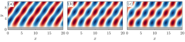
(a)

(b)

(c)

Figure 15: The pressure fluctuations obtained from the leading resolvent response for a supersonic mode is shown with the red and blue contours representing positive and negative pressure fluctuations, respectively. The mode corresponds to $\lambda_{x}=5$, $\lambda_{z}=3.5$ and $c=\overline{U}(y^{+}\approx 15)$ for a compressible boundary layer over an adiabatic wall with $Ma=4$ and $Re_{\tau}=400$ (the mode indicated by the ($\blacksquare$) in figure 1(b)). The strength of the damping layer used increases from (a) $0.15$ to (b) $0.5$ and then to (c) $1.5$.

It is important to consider if the grid stretching and the introduction of the damping layer impacts the conclusions drawn in the current work. To investigate this, in figure 14 the real and the imaginary parts of the pressure obtained from the leading resolvent response for the supersonic mode $\lambda_{x}=5$, $\lambda_{y}=3.5$ and $c\approx U(y^{+}=15)$ is shown. Three grids are considered in figure 14: (i) Case 1 (grey solid line): the same grid as that used in this work, but without a damping layer, (ii) Case 2 (red solid line): the grid used in this work with $N=401$ and $y_{max}=4\delta$ for the subsonic modes and $y_{max}=3l$ for the supersonic modes (where $l$ is the wavelength of the Mach waves) and (iii) Case 3 (blue dashed line): with $N=601$ and $y_{max}=5\delta$ for the subsonic modes and $y_{max}=4l$ for the supersonic modes. The red shaded regions towards the free-stream indicates the extent of the damping-layer for Case 2, and the blue shaded region indicates the damping layer for Case 3 (since the number of points in the damping layer is fixed to be $20$, the wall-normal extent of the damping layer changes with $N$). To keep the comparison consistent across the three cases, all the responses are set to zero within the red shaded region and beyond into the freestream. Considering the grey lines from Case 1, where no damping layer or artificial viscosity is included, we observe saw-tooth oscillations that arise due to the grid stretching. From the modes obtained with damping layers we note that this damping removes the saw-tooth oscillations. Comparing the responses from Case 2 and Case 3, we notice that there are small differences between the modes. This is probably expected given that the extent of the damping layer is different for the two cases. Importantly, these differences do not impact the conclusions drawn in the current work. To see this, in figures 16(16(a)-16(c)) we reproduce figures 12(12(a)-12(c)) using more number of grid points and a larger $y_{max}$. In other words, the data plotted in figures 16(16(a)-16(c)) are computed using the grid Case 3, while the data in figures 12(12(a)-12(c)) were computed using the grid Case 2. We see that there are no significant differences that arise due to an increase in the number of grid points as well as an increase in the maximum extent of the wall-normal grid.

To investigate the effect of the damping-layer a little further, in figure 15 the real part of the pressure obtained using the grid Case 2 is shown, with the strength of the artificial viscosity increasing moving from left to right. We notice that there is a beating in the pressure fluctuations, that is made worse as the strength of this artificial viscosity increases. This is likely due to reflections introduced by the artificial viscosity. This shows that we should exercise caution while introducing artificial viscosity (removing the artificial viscosity is not a valid option since it will re-introduce the saw-tooth oscillations). However, the results in the current work are not affected by the strength of the artificial viscosity. To illustrate this, in figures 16(16(d)-16(f)) we reproduce figures 12(12(a)-12(c)) with a grid that uses a stronger artificial viscosity (the strength is determined by the value of $\gamma_{k}$ which is increased from $0.15$ in figures 12(12(a)-12(c)) to $1.5$ in figures 16(16(d)-16(f))). There are no significant differences that are introduced by this change in the strength of the damping layer.

We can therefore conclude that the main conclusions drawn in the current work are not significantly impacted by changes in the grid used.

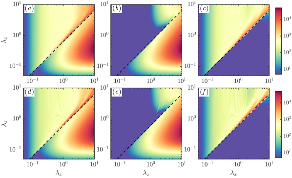
(a)

(b)

(c)

(d)

(e)

(f)

Figure 16: The Chu norm of the response of the resolvent operator to (a,d) the full leading resolvent forcing mode $\bm{\phi}_{1}$ as well as the two components of the forcing (b,e) $\widehat{\bm{f}}_{1}$ and (c,f) $\widehat{\bm{f}}_{2}$ are shown as a function of the streamwise ($\lambda_{x}$) and spanwise ($\lambda_{z}$) wavelengths for a fixed value of phase speed $c=\overline{U}(y^{+}\approx 15)$. The $Ma=4$, $Re_{\tau}=400$ turbulent boundary layer over an adiabatic wall (that was also considered in figure 12) is shown here. (a-c) The responses obtained using $N=601$ grid points and a $y_{max}=5\delta$ in the subsonic region and $y_{max}=4l$ in the supersonic region is shown. (d-f) Also shown are the responses obtained with a grid where the strength of the damping layer is increased to $\gamma_{k}=1.5$ (from the $\gamma_{k}=0.15$ used for figure 12). These responses are compared to those shown in figures 12(12(a)-12(c)) to illustrate the insensitivity of the obtained results to the grid used. The dashed lines in all figures indicate the relative Mach equal to unity line.

References

- Appelö & Colonius (2009) Appelö, D. & Colonius, T. 2009 A high-order super-grid-scale absorbing layer and its application to linear hyperbolic systems. J. Comput. Phys. 228 (11), 4200–4217.
- Bae et al. (2020a) Bae, H. J., Dawson, S. T. & McKeon, B. J. 2020a Studying the effect of wall cooling in supersonic boundary layer flow using resolvent analysis. In AIAA Scitech 2020 Forum, p. 0575.
- Bae et al. (2020b) Bae, H. J., Dawson, S. T. M. & McKeon, B. J. 2020b Resolvent-based study of compressibility effects on supersonic turbulent boundary layers. J. Fluid Mech. 883.
- Balakumar & Malik (1992) Balakumar, P. & Malik, M. R. 1992 Discrete modes and continuous spectra in supersonic boundary layers. J. Fluid Mech. 239, 631–656.
- Bertolotti et al. (1992) Bertolotti, F. P., Herbert, T. & Spalart, P. R. 1992 Linear and nonlinear stability of the Blasius boundary layer. J. Fluid Mech. 242, 441–474.
- Bitter & Shepherd (2014) Bitter, N. & Shepherd, J. 2014 Transient growth in hypersonic boundary layers. In 7th AIAA Theoretical Fluid Mechanics Conference, p. 2497.
- Bitter & Shepherd (2015) Bitter, N. P. & Shepherd, J. E. 2015 Stability of highly cooled hypervelocity boundary layers. J. Fluid Mech. 778, 586–620.
- Bross et al. (2021) Bross, M., Scharnowski, S. & Kähler, C. J. 2021 Large-scale coherent structures in compressible turbulent boundary layers. J. Fluid Mech. 911.
- Bugeat et al. (2019) Bugeat, B., Chassaing, J.-C., Robinet, J.-C. & Sagaut, P. 2019 3D global optimal forcing and response of the supersonic boundary layer. J. Comput. Phys. 398, 108888.
- Chang et al. (1991) Chang, C.-L., Malik, M., Erlebacher, G. & Hussaini, M. 1991 Compressible stability of growing boundary layers using parabolized stability equations. AIAA Paper pp. 91–1636.
- Chu (1965) Chu, B.-T 1965 On the energy transfer to small disturbances in fluid flow (Part i). Acta Mech. 1 (3), 215–234.
- Cook et al. (2018) Cook, D. A., Thome, J., Brock, J. M., Nichols, J. W. & Candler, G. V. 2018 Understanding effects of nose-cone bluntness on hypersonic boundary layer transition using input-output analysis. In 2018 AIAA Aerospace Sciences Meeting, AIAA Paper, p. 0378.
- Dawson & McKeon (2019) Dawson, S. T. M. & McKeon, B. J. 2019 Studying the effects of compressibility in planar Couette flow using resolvent analysis. In AIAA SciTech, p. 2139.
- Dawson & McKeon (2020) Dawson, S. T. M. & McKeon, B. J. 2020 Prediction of resolvent mode shapes in supersonic turbulent boundary layers. Int. J. Heat Fluid Flow 85, 108677.
- Donaldson & Coulter (1995) Donaldson, J. & Coulter, S. 1995 A review of free-stream flow fluctuation and steady-state flow quality measurements in the AEDC/VKF supersonic tunnel A and hypersonic tunnel B. AIAA Paper p. 6137.
- Duan et al. (2010) Duan, L., Beekman, I. & Martín, M. P. 2010 Direct numerical simulation of hypersonic turbulent boundary layers. Part 2. Effect of wall temperature. J. Fluid Mech. 655, 419.
- Duan et al. (2011) Duan, L, Beekman, I. & Martín, M. P. 2011 Direct numerical simulation of hypersonic turbulent boundary layers. Part 3. Effect of Mach number. J. Fluid Mech. 672, 245.
- Duan et al. (2014) Duan, L., Choudhari, M. M. & Wu, M. 2014 Numerical study of acoustic radiation due to a supersonic turbulent boundary layer. J. Fluid Mech. 746, 165–192.
- Duan et al. (2016) Duan, L., Choudhari, M. M & Zhang, C. 2016 Pressure fluctuations induced by a hypersonic turbulent boundary layer. J. Fluid Mech. 804, 578–607.
- Duan & Martin (2011) Duan, L. & Martin, M. P. 2011 Direct numerical simulation of hypersonic turbulent boundary layers. Part 4. Effect of high enthalpy. J. Fluid Mech. 684, 25.
- Dwivedi et al. (2018) Dwivedi, A., Sidharth, G. S., Candler, G. V., Nichols, J. W. & Jovanović, M. R. 2018 Input-output analysis of shock boundary layer interaction. In 2018 Fluid Dynamics Conference, p. 3220.
- Dwivedi et al. (2019) Dwivedi, A., Sidharth, G. S., Nichols, J. W., Candler, G. V. & Jovanović, M. R. 2019 Reattachment streaks in hypersonic compression ramp flow: an input–output analysis. J. Fluid Mech. 880, 113–135.
- Ellingsen & Palm (1975) Ellingsen, T. & Palm, E. 1975 Stability of linear flow. Phys. Fluids 18 (4), 487–488.
- Fedorov (2011) Fedorov, A. 2011 Transition and stability of high-speed boundary layers. Annu. Rev. Fluid Mech. 43, 79–95.
- Fedorov & Tumin (2011) Fedorov, A. & Tumin, A. 2011 High-speed boundary-layer instability: old terminology and a new framework. AIAA J. 49 (8), 1647–1657.
- Ffowcs Williams (1963) Ffowcs Williams, J. E. 1963 The noise from turbulence convected at high speed. Phil. Trans. R. Soc. Lond. 255 (1061), 469–503.
- Ganapathisubramani et al. (2006) Ganapathisubramani, B., Clemens, N. T. & Dolling, D. S. 2006 Large-scale motions in a supersonic turbulent boundary layer. J. Fluid Mech. 556, 271.
- Govindarajan & Narasimha (1995) Govindarajan, R. & Narasimha, R. 1995 Stability of spatially developing boundary layers in pressure gradients. J. Fluid Mech. 300, 117–147.
- Hanifi & Henningson (1998) Hanifi, A. & Henningson, D. S. 1998 The compressible inviscid algebraic instability for streamwise independent disturbances. Phys. Fluids 10 (8), 1784–1786.
- Hanifi et al. (1996) Hanifi, A., Schmid, P. J. & Henningson, D. S. 1996 Transient growth in compressible boundary layer flow. Phys. Fluids 8 (3), 826–837.
- Hu et al. (2006) Hu, Z., Morfey, C. L. & Sandham, N. D. 2006 Sound radiation from a turbulent boundary layer. Phys. Fluids 18 (9), 098101.
- Illingworth (2019) Illingworth, S. J. 2019 Streamwise-constant large-scale structures in Couette and Poiseuille flows. arXiv preprint arXiv:1904.10603 .
- Jovanović & Bamieh (2005) Jovanović, M. R. & Bamieh, B. 2005 Componentwise energy amplification in channel flows. J. Fluid Mech. 534, 145–183.
- Kamal et al. (2021) Kamal, O., Rigas, G., Lakebrink, M. & Colonius, T. 2021 Input/output analysis of hypersonic boundary layers using the one-way navier-stokes (OWNS) equations. In AIAA AVIATION 2021 FORUM, p. 2827.
- Kamal et al. (2020) Kamal, O., Rigas, G., Lakebrink, M. T. & Colonius, T. 2020 Application of the One-Way Navier-Stokes (OWNS) equations to hypersonic boundary layers. In AIAA AVIATION 2020 FORUM, p. 2986.
- Kendall (1970) Kendall, J. M. 1970 Supersonic boundary layer transition studies. JPL Space Programs Summary 3, 43–47.
- Kline et al. (1967) Kline, S. J., Reynolds, W. C., Schraub, F. A. & Runstadler, P. W. 1967 The structure of turbulent boundary layers. J. Fluid Mech. 30 (04), 741–773.
- Lagha et al. (2011) Lagha, M., Kim, J., Eldredge, J. D. & Zhong, X. 2011 A numerical study of compressible turbulent boundary layers. Phys. Fluids 23 (1), 015106.
- Laufer (1961) Laufer, J. 1961 Sound radiation from a turbulent boundary layer. Tech. Rep..
- Laufer (1964) Laufer, J. 1964 Some statistical properties of the pressure field radiated by a turbulent boundary layer. Phys. Fluids 7 (8), 1191–1197.
- Lees & Lin (1946) Lees, L. & Lin, C. C. 1946 Investigation of the stability of the laminar boundary layer in a compressible fluid. National Advisory Committee for Aeronautics.
- Lees & Reshotko (1962) Lees, L. & Reshotko, E. 1962 Stability of the compressible laminar boundary layer. J. Fluid Mech. 12 (4), 555–590.
- Ma & Zhong (2003) Ma, Y. & Zhong, X. 2003 Receptivity of a supersonic boundary layer over a flat plate. Part 1. wave structures and interactions. J. Fluid Mech. 488, 31–78.
- Mack (1965) Mack, L. M. 1965 Computation of the stability of the laminar boundary layer. Methods in Computational Physics 4, 247–299.
- Mack (1975) Mack, L. M. 1975 Linear stability theory and the problem of supersonic boundary-layer transition. AIAA J. 13 (3), 278–289.
- Mack (1984) Mack, L. M. 1984 Boundary-layer linear stability theory. Tech. Rep.. California Inst of Tech Pasadena Jet Propulsion Lab.
- Malik et al. (2008) Malik, M., Dey, J. & Alam, M. 2008 Linear stability, transient energy growth, and the role of viscosity stratification in compressible plane Couette flow. Phys. Rev. E 77 (3), 036322.
- Malik (1990) Malik, M. R. 1990 Numerical methods for hypersonic boundary layer stability. J. Comput. Phys. 86 (2), 376–413.
- Mattsson & Nordström (2004) Mattsson, K. & Nordström, J. 2004 Summation by parts operators for finite difference approximations of second derivatives. J. Comput. Phys. 199 (2), 503–540.
- McKeon & Sharma (2010) McKeon, B. J. & Sharma, A. S. 2010 A critical-layer framework for turbulent pipe flow. J. Fluid Mech. 658, 336–382.
- Moarref et al. (2014) Moarref, R., Jovanović, M. R., Tropp, J. A., Sharma, A. S. & McKeon, B. J. 2014 A low-order decomposition of turbulent channel flow via resolvent analysis and convex optimization. Phys. Fluids 26 (5), 051701.
- Moarref et al. (2013) Moarref, R., Sharma, A. S., Tropp, J. A. & McKeon, B. J. 2013 Model-based scaling of the streamwise energy density in high-Reynolds number turbulent channels. J. Fluid Mech. 734, 275–316.
- Morra et al. (2021) Morra, P., Nogueira, P. A. S., Cavalieri, A. V. G. & Henningson, D. S. 2021 The colour of forcing statistics in resolvent analyses of turbulent channel flows. Journal of Fluid Mechanics 907.
- Nogueira et al. (2020) Nogueira, P. A. S., Cavalieri, A. V. G., Hanifi, A. & Henningson, D. S. 2020 Resolvent analysis in unbounded flows: role of free-stream modes. Theor. Comput. Fluid Dyn. 34 (1), 163–176.
- Özgen & Kırcalı (2008) Özgen, S. & Kırcalı, S. A. 2008 Linear stability analysis in compressible, flat-plate boundary-layers. Theor. Comput. Fluid Dyn. 22 (1), 1–20.
- Paredes et al. (2016) Paredes, P., Choudhari, M. M., Li, F. & Chang, C.-L. 2016 Optimal growth in hypersonic boundary layers. AIAA J. 54 (10), 3050–3061.
- Pate (1978) Pate, S. R. 1978 Dominance of radiated aerodynamic noise on boundary-layer transition in supersonic-hypersonic wind tunnels. Theory and application. Tech. Rep.. Arnold Engineering Development Center Arnold AFB TN.
- Pate & Schueler (1969) Pate, S. R. & Schueler, C. J. 1969 Radiated aerodynamic noise effects on boundary-layer transition in supersonic and hypersonic wind tunnels. AIAA J. 7 (3), 450–457.
- Phillips (1960) Phillips, O. M. 1960 On the generation of sound by supersonic turbulent shear layers. J. Fluid Mech. 9 (1), 1–28.
- Pirozzoli & Bernardini (2011) Pirozzoli, S. & Bernardini, M. 2011 Turbulence in supersonic boundary layers at moderate Reynolds number. J. Fluid Mech. 688, 120.
- Ran et al. (2019) Ran, W., Zare, A., Hack, M. J. P. & Jovanović, M. R. 2019 Stochastic receptivity analysis of boundary layer flow. Phys. Rev. Fluids 4 (9), 093901.
- Rosenberg & McKeon (2019) Rosenberg, K. & McKeon, B. J. 2019 Efficient representation of exact coherent states of the Navier–Stokes equations using resolvent analysis. Fluid Dyn. Res. 51 (1), 011401.
- Ruan & Blanquart (2021) Ruan, J. & Blanquart, G. 2021 Direct numerical simulations of a statistically stationary streamwise periodic boundary layer via the homogenized Navier-Stokes equations. Phys. Rev. Fluids 6 (2), 024602.
- Schneider (2001) Schneider, Steven P 2001 Effects of high-speed tunnel noise on laminar-turbulent transition. J. of Spacecr. and Rockets 38 (3), 323–333.
- Sharma & McKeon (2013) Sharma, A. S. & McKeon, B. J. 2013 On coherent structure in wall turbulence. J. Fluid Mech. 728, 196–238.
- Smits & Dussauge (2006) Smits, A. J. & Dussauge, J.-P. 2006 Turbulent shear layers in supersonic flow. Springer Science & Business Media.
- Smits et al. (2011) Smits, A. J., McKeon, B. J. & Marusic, I. 2011 High-Reynolds number wall turbulence. Annu. Rev. Fluid Mech. 43, 353–375.
- Smits et al. (1989) Smits, A. J., Spina, E. F., Alving, A. E., Smith, R. W., Fernando, E. M. & Donovan, J. F. 1989 A comparison of the turbulence structure of subsonic and supersonic boundary layers. Phys. Fluids A 1 (11), 1865–1875.
- Stainback (1971) Stainback, P. C. 1971 Hypersonic boundary-layer transition in the presence of wind-tunnel noise. AIAA J. 9 (12), 2475–2476.
- Tempelmann et al. (2012) Tempelmann, D., Hanifi, A. & Henningson, D. 2012 Spatial optimal growth in three-dimensional compressible boundary layers. J. Fluid Mech. 704, 251–279.
- Thompson (1987) Thompson, K. W. 1987 Time dependent boundary conditions for hyperbolic systems. J. Comput. Phys. 68 (1), 1–24.
- Towne et al. (2020) Towne, A., Lozano-Durán, A. & Yang, X. 2020 Resolvent-based estimation of space–time flow statistics. J. Fluid Mech. 883.
- Trettel & Larsson (2016) Trettel, A. & Larsson, J. 2016 Mean velocity scaling for compressible wall turbulence with heat transfer. Phys. Fluids 28 (2), 026102.
- Tumin & Reshotko (2001) Tumin, A. & Reshotko, E. 2001 Spatial theory of optimal disturbances in boundary layers. Phys. Fluids 13 (7), 2097–2104.
- Tumin & Reshotko (2003) Tumin, A. & Reshotko, E. 2003 Optimal disturbances in compressible boundary layers. AIAA J. 41 (12), 2357–2363.
- Wagner Jr et al. (1970) Wagner Jr, R. D., Maddalon, D. V. & Weinstein, L. M. 1970 Influence of measured freestream disturbances on hypersonic boundary-layer transition. AIAA J. 8 (9), 1664–1670.
- Williams et al. (2018) Williams, O. J. H., Sahoo, D., Baumgartner, M. L. & Smits, A. J. 2018 Experiments on the structure and scaling of hypersonic turbulent boundary layers. J. Fluid Mech. 834, 237–270.
- Yu et al. (2019) Yu, M., Xu, C.-X. & Pirozzoli, S. 2019 Genuine compressibility effects in wall-bounded turbulence. Phys. Rev. Fluids 4 (12), 123402.
- Yu et al. (2020) Yu, M., Xu, C.-X. & Pirozzoli, S. 2020 Compressibility effects on pressure fluctuation in compressible turbulent channel flows. Phys. Rev. Fluids 5 (11), 113401.
- Zare et al. (2017) Zare, A., Jovanović, M. R. & Georgiou, T. T. 2017 Colour of turbulence. J. Fluid Mech. 812, 636–680.
- Zhang et al. (2017) Zhang, C., Duan, L. & Choudhari, M. M. 2017 Effect of wall cooling on boundary-layer-induced pressure fluctuations at Mach 6. J. Fluid Mech. 822, 5–30.
- Zuccher et al. (2006) Zuccher, S., Tumin, A. & Reshotko, E. 2006 Parabolic approach to optimal perturbations in compressible boundary layers. J. Fluid Mech. 556, 189–216.