Quantum Hall Phases of Cold Bose Gases

Nicolas Rougerie

Ecole Normale Supérieure de Lyon & CNRS, UMPA (UMR 5669)
E-mail: nicolas.rougerie@ens-lyon.fr

Jakob Yngvason

Fakultät für Physik, Universität Wien, Boltzmanngasse 5, 1090 Vienna, Austria
Erwin Schrödinger Institute for Mathematics and Physics, Boltzmanngasse 9, 1090 Vienna, Austria.
E-mail: jakob.yngvason@univie.ac.at

Abstract Cold atomic gases of interacting bosons subject to rapid rotation and confined in anharmonic traps can theoretically exhibit analogues of the fractional quantum Hall effect for electrons in strong magnetic fields. In this setting the Coriolis force due to the rotation mimics the Lorentz force on charged particles but artificial gauge fields can also be obtained by coupling the internal structure of the atoms to light fields. The chapter discusses mathematical aspects of transitions to different strongly correlated phases that appear when the parameters of a model Hamiltonian are varied.

Keywords. Cold Bose gases, rapid rotation, anharmonic traps, fractional quantum Hall effect for bosons, Laughlin wave function, yrast curve, spectral gap conjecture, strongly correlated phases, plasma analogy.

1 Key objectives

• Define a model Hamiltonian for trapped, interacting bosons in rapid rotation.

• Describe the confinement to the lowest Landau level for the kinetic part of the Hamiltonian.

• Discuss the yrast curve and the transition from an uncorrelated ground state in the lowest Landau level to fractional quantum Hall states.

• Discuss transitions from a Laughlin state to other strongly correlated states including giant vortex states in anharmonic traps.

• Derive density profiles of the strongly correlated states by means of Laughlin’s plasma analogy and rigorous mean field theory.

2 Notations and acronyms

$\Omega_{\rm trap}$: Frequency of a harmonic trap.
$\Omega_{\rm rot}$: Rotational frequency.
$\omega=\Omega_{\rm trap}-\Omega_{\rm rot}$: Frequency difference.
$\mathbf{L}$: Angular momentum.
$V^{\parallel}$: Transverse confining potential.
$e^{\parallel}$: Spectral gap of the transverse confinement.
$\mathcal{L}=\mathbf{e}_{3}\cdot\mathbf{L}$: Transverse component of angular momentum.
LLL: Lowest Landau level.

3 Introduction

Since the early 1990’s it has been possible to isolate ultra-cold atomic gases of bosons in magneto-optical traps and maintain them in metastable states that can be modelled as ground states of many-body Hamiltonians with repulsive short range interactions. At sufficiently low temperatures the gas forms a Bose-Einstein condensate (BEC) (Ketterle et al (1996); Cornish et al (2000)) with all the atoms in the same state that can for dilute gases be described by an effective single particle equation of Gross-Pitaevskii type (Pethick & Smith (2008); Pitaevskii & Stringari (2016)).

The atoms usually have no electric charge, but an artificial magnetic field can be imposed on them by a steady rotation of the trap. The analogy between the Lorentz and Coriolis forces implies that the Hamiltonian for neutral atoms in a rotating trap is formally identical to that of charged particles in a uniform magnetic field, apart from the centrifugal potential associated with the rotation. The analogy shows up, in particular, in the emergence of quantized vortices in cold rotating Bose gases (Bretin et al (2004); Aftalion (2006); Cooper (2008); Fetter (2009); Correggi et al (2011)), similar to those appearing in type II superconductors submitted to external magnetic fields.

An even more striking possibility is to employ rapid rotation to create phases with the characteristics of the fractional quantum Hall effect (FQHE) for electrons in very large magnetic fields (Prange & Girvin (1987); Chakraborty & Pietiläinen (1988, 1995); Störmer et al (1999); Jain (2007)). In this regime, the Bose gas is no longer a condensate and mean-field theories fail to capture this phenomenon. A truly many-body description is required and strongly correlated states, such as the celebrated Laughlin state (Laughlin (1983)), may theoretically occur. This requires, however that the Coriolis force is very strong which inevitably means that the centrifugal force is also strong and may outweigh the trapping force. This can lead to an instability of the system unless special countermeasures are taken (Bretin et al (2004); Schweikhard et al (2004); Viefers (2008); Fetter (2009)). In fact, the competing demands of a large rotation speed on the one hand, necessary for entering the FQHE regime, and of a sufficiently stable system on the other hand, have so far left the FQHE regime in rotating gases unattainable with current technology. Alternative methods to create artifical gauge fields have therefore been proposed and even partly realized in experiments (Dalibard et al (2011); Roncaglia et al (2011); Clark et al (2020); Hauke & Carusotto (2022)).

From a theoretical point of view, however, the use of an anharmonic trapping potential to beat the destabilizing effect of the Coriolis force in a rotating trap remains a conceptually simple road to strongly correlated phases of Bosons with short range interactions. In this chapter we shall discuss how different phases may be produced by varying the parameters in this set-up. The same conclusions will apply to other experimental realizations of the Hamiltonian whenever they can be achieved.

4 The basic Hamiltonian

We consider first the following many-body Hamiltonian for $N$ bosons of unit mass with position vectors ${\bf x}_{(1)},\dots\bf x_{(N)}$ in a rotating frame of reference:

$$H_{N}=\sum_{i=1}^{N}\left(-\mbox{$\frac{1}{2}$}\nabla^{2}_{(i)}+V({\bf x}_{(i)})-{\mathbf{L}}_{(i)}\cdot{{\mathbf{\Omega}}}\right)+\sum_{1\leq i<j\leq N}v(|{\bf x}_{(i)}-{\bf x}_{(j)}|).$$ (1)

Here $\mathbf{\Omega}=\Omega_{\rm rot}\mathbf{e}_{3}$ is the angular velocity, with $\mathbf{e}_{3}$ the unit vector in the 3-direction and with $\Omega_{\rm rot}\geq 0$, $\mathbf{L}=-\mathrm{i}\mathbf{{\bf x}}\times\nabla$ the angular momentum operator,

$$V({\bf x})=\mbox{$\frac{1}{2}$}\Omega_{\rm trap}^{2}r^{2}+V^{\parallel}(x_{3})$$ (2)

with ${\bf x}=(x_{1},x_{2},x_{3})$, $r^{2}=(x_{1})^{2}+(x_{2})^{2}$, a quadratic trapping potential in the 12-plane, $V^{\parallel}$ a confining positive potential in the 3-direction, and $v$ the pair interaction potential, assumed to be $\geq 0$. Units have been chosen so that Planck constant $\hbar$ as well as the particle mass is 1.

It is convenient to define the gauge field as

$$\mathbf{A}({\bf x})=\Omega_{\rm trap}(x_{2},-x_{1},0)$$ (3)

and write the Hamiltonan (1) as

$$H_{N}=\sum_{j=1}^{N}\left\{\mbox{$\frac{1}{2}$}(\mathrm{i}\nabla_{(j)}+\mathbf{A}({\bf x}_{(j)}))^{2}+\omega\,\mathbf{e}_{3}\cdot\mathbf{L}_{(j)}+V^{\parallel}(x_{3})\right\}+\sum_{i<j}v(|{\bf x}_{(i)}-{\bf x}_{(j)}|)$$ (4)

with

$$\omega=\Omega_{\rm trap}-\Omega_{\rm rot}.$$ (5)

We are interested in the case that $\omega>0$ is small and $\Omega_{\rm rot}$ (hence also $\Omega_{\rm trap}$) is large.

4.1 Confinement to the Lowest Landau Level

4.1.1 The 1-particle case

The single-particle Hamiltonian

$$H_{1}=\mbox{$\frac{1}{2}$}(\mathrm{i}\nabla_{\perp}+\mathbf{A}({\bf x}))^{2}+\omega\mathcal{L}-\mbox{$\frac{1}{2}$}\partial_{3}^{2}+V^{\parallel}(x_{3})$$ (6)

with the notation $\mathcal{L}=\mathbf{e}_{3}\cdot\mathbf{L}$ and $\nabla_{\perp}=(\partial_{1},\partial_{2})$, is a sum of three commuting operators,

$$\mbox{$\frac{1}{2}$}(\mathrm{i}\nabla_{\perp}+\mathbf{A}({\bf x}))^{2}$$ (7)

$$\omega\mathcal{L}$$ (8)

$$-\mbox{$\frac{1}{2}$}\partial_{3}^{2}+V^{\parallel}(x_{3}).$$ (9)

The first operator, $\mbox{$\frac{1}{2}$}(\mathrm{i}\nabla_{\perp}+\mathbf{A}({\bf x}))^{2}$, has the form of a magnetic Hamiltonian with the Landau spectrum

$$(n+\mbox{$\frac{1}{2}$})\mathrm{2}\Omega_{\rm trap},\quad n=\mathrm{0,1,2},\dots,.$$ (10)

The spectrum of $\omega\mathcal{L}$ is

$$\ell\omega,\quad\ell=0,\pm 1,\pm 2\dots$$ (11)

and $-\mbox{$\frac{1}{2}$}\partial_{3}^{2}+V^{\parallel}(x_{3})$ has a spectral gap, $e^{\parallel}>0$, above its ground state.

The energy of (6) is minimized in states with $n=0$, i.e., in the lowest Landau level (LLL) of the magnetic Hamiltonian. Moreover, in the lowest energy state the motion in the $x_{3}$-direction is ‘frozen’ in the ground state of $h^{\parallel}$. Confinement to the LLL in the $N$-particle context, taking the repulsive interaction into account, is discussed in subsection 4.1.3 below.

From now on we focus on the 2-dimensional motion in the 12-plane and choose units so that $\Omega_{\rm trap}=1$.

4.1.2 Complex notation and Bargmann space

It is convenient to adopt complex notation for the position variables. Replacing $(x_{1},x_{2})$ by the complex coordinate $z=x_{1}+\mathrm{i}x_{2}$ and denoting $\partial=\mbox{$\frac{1}{2}$}(\partial_{1}-\mathrm{i}\partial_{2})$, $\bar{\partial}=\mbox{$\frac{1}{2}$}(\partial_{1}+\mathrm{i}\partial_{2})$ we can write

$$\mbox{$\frac{1}{2}$}(\mathrm{i}\nabla_{\perp}+\mathbf{A}({\bf x}))^{2}=2\left(\hat{a}^{\dagger}\hat{a}+\mbox{$\frac{1}{2}$}\right)$$ (12)

with

$$\hat{a}^{\dagger}:=\mbox{$\frac{1}{2}$}(-2\partial+\bar{z}),\qquad\hat{a}:=\mbox{$\frac{1}{2}$}(2\bar{\partial}+z).$$ (13)

These operators satisfy the canonical commutation relations

$$[\hat{a},\hat{a}^{\dagger}]=1.$$ (14)

The operators

$$\hat{b}^{\dagger}:=\mbox{$\frac{1}{2}$}(-2\bar{\partial}+z),\qquad\hat{b}:=\mbox{$\frac{1}{2}$}(2\partial+\bar{z})$$ (15)

also satisfy the canonical commutation relations and commute with $\hat{a}$ and $\hat{a}^{\dagger}$. They correspond to a replacement $\mathbf{A}\to-\mathbf{A}$:

$$\mbox{$\frac{1}{2}$}(\mathrm{i}\nabla_{\perp}-\mathbf{A}({\bf x}))^{2}=2(\hat{b}^{\dagger}\hat{b}+\mbox{$\frac{1}{2}$}).$$ (16)

Moreover,

$$\hat{b}^{\dagger}\hat{b}-\hat{a}^{\dagger}\hat{a}=z\partial-\bar{z}\bar{\partial}=\mathcal{L}.$$ (17)

Hence the eigenvalues of $\hat{a}^{\dagger}\hat{a}$ are infinitely degenerate and the degenerate eigenstates can be labelled by eigenvalues of either $\hat{b}^{\dagger}\hat{b}$ or $\mathcal{L}$.

The lowest eigenvalue of $\hat{a}^{\dagger}\hat{a}$ is zero so the eigenfunctions $\psi(z,\bar{z})$ in the LLL are solutions of the equation $\hat{a}\psi=0$, i.e.,

$$\bar{\partial}\psi(z,\bar{z})=-\mbox{$\frac{1}{2}$}z\psi(z,\bar{z}).$$ (18)

This means that

$$\psi(z,\bar{z})=\varphi(z)\exp(-|z|^{2}/2)$$ (19)

with $\bar{\partial}\varphi(z)=0$, i.e., $\varphi$ is an analytic (holomorphic) function of $z$.

The LLL can thus be regarded as the Bargmann space $\mathcal{B}$ (Bargmann (1961); Girvin & Jach (1984)) of analytic functions $\varphi$ such that

$$\langle\varphi,\varphi\rangle:=\int|{\varphi(z)}|^{2}\exp(-|z|^{2})\,\mathrm{d}^{2}z<\infty$$ (20)

where $\,\mathrm{d}^{2}z$ denotes the Lebesgue measure on $\mathbb{C}$ (regarded as $\mathbb{R}^{2}$).

The Bargmann space is a Hilbert space with scalar product

$$\langle\varphi,\psi\rangle:=\int\bar{\varphi}(z)\psi(z)\exp(-|z|^{2})\,\mathrm{d}^{2}z.$$ (21)

On $\mathcal{B}$ the angular momentum operator is $\mathcal{L}=z\partial$. Moreover, for $\varphi\in\mathcal{B}$,

$$\langle\varphi,\mathcal{L}\varphi\rangle=\int(|z|^{2}-1)\,|{\varphi(z)}|^{2}\exp(-|z|^{2})\,\mathrm{d}^{2}z.$$ (22)

The eigenvalues of $\mathcal{L}$ restricted to $\mathcal{B}$ are $\ell=0,1,2,\dots$ with corresponding normalized eigenfunctions

$$\varphi_{\ell}(z)=\left(\pi\ell!\right)^{-1/2}\,z^{\ell}.$$ (23)

By (22) the probability density $|\varphi_{\ell}(z)|^{2}e^{-|z|^{2}}$ is localized around $|z|=\sqrt{\ell+1}$.

4.1.3 The $N$-particle case, contact interaction

For $N$ bosons in the LLL the relevant Hilbert space is

$$\mathcal{B}_{N}=\mathcal{B}^{\otimes^{N}_{\rm symm}},$$ (24)

i.e., it consists of symmetric, analytic functions $\psi$ of $z_{1},\dots,z_{N}$ such that

$$\int_{\mathbb{C}^{N}}|\psi(z_{1},\dots,z_{N})|^{2}\exp\Big{(}-\sum_{j=1}^{N}|z_{j}|^{2}\Big{)}\,\mathrm{d}^{2}z_{1}\cdots\,\mathrm{d}^{2}z_{N}<\infty.$$ (25)

As next we take the interaction $\sum_{1\leq i<j\leq N}v(|{\bf x}_{i}-{\bf x}_{j}|)$ into account,

For short range, nonnegative interaction potentials $v$ it was proved in (Lewin & Seiringer (2009)) that under suitable conditions on $N$, $v$ and $\omega$:

• The ground state of (6) is effectively confined to the LLL in the 12-variables and in the 3-direction to the the ground state of (9).

• The interaction potential $v$ can be replaced by a contact interaction (pseudopotential) in the 12-variables of the form $g\delta(z_{i}-z_{j})$ with a coupling constant

  $$g=a\cdot\sqrt{e^{\parallel}}\hbox{$\int|\chi|^{4}$}$$ (26)

  where $a$ is the $s$-wave scattering length of the potential $v$ and $\chi$ the ground state wave function of (9).

Precise statements are contained in Theorems 1 and 2 in Lewin & Seiringer (2009). For the emergence of the pseudopotential see also (Seiringer & Yngvason (2020)), Theorem 2. Since wave functions in the Bargmann space $\mathcal{B}_{N}$ are analytic, the 2-body contact potential $\delta(z_{i}-z_{j})$ is well defined and, in fact, given by a bounded operator: Defining $\delta_{12}$ on $\mathcal{B}_{2}$ by

$$\delta_{12}\varphi(z_{1},z_{2})=\frac{1}{2\pi}\varphi\big{(}\mbox{$\frac{1}{2}$}(z_{1}+z_{2}),\mbox{$\frac{1}{2}$}(z_{1}+z_{2})\big{)},$$ (27)

a simple computation, using the analyticity of $\varphi$, shows that

$$\langle\varphi,\delta_{12}\varphi\rangle=\int_{\mathbb{C}}|{\varphi(z,z)}|^{2}\exp(-2|z|^{2})\,\mathrm{d}^{2}z.$$ (28)

Thus the formal $\delta(z_{i}-z_{j})$ can be replaced by the projection operator $\delta_{ij}$. The effective Hamiltonian on the LLL can be written as

$$\boxed{H_{N}^{\rm LLL}={\omega}\,\mathcal{L}_{N}+{g}\,\mathcal{I}_{N}}$$ (29)

with

$$\mathcal{L}_{N}=\sum_{i=1}^{N}z_{i}\partial_{i}\,\quad\quad\mathcal{I}_{N}=\sum_{i<j}\delta_{ij}.$$ (30)

We denote its ground state energy by $E_{N}^{\rm LLL}(\omega,g)$.

Writing $v({\bf x})=v_{a}({\bf x})=a^{-2}v_{1}({\bf x}/a)$ and keeping $v_{1}$ fixed while varying $a$, we denote by by $E_{N}(\omega,a)$ the ground state energy of (1) with $N$ $\times$ the lowest energy of (7) and (9) subtracted. Then Theorem 1 in Lewin & Seiringer (2009) states that

$$\lim\frac{E_{N}(\omega,a)}{E_{N}^{\rm LLL}(\omega,g)}=1$$ (31)

in a limit where

$$(Ng\omega)^{1/2}\ll\min\{\Omega_{\rm trap},e^{\parallel}\}.$$ (32)

Moreover, in the same limit also the ground state converges to its projection onto the LLL (Theorem 2 in Lewin & Seiringer (2009)).

4.2 The yrast curve

An important property of the Hamiltonian (29) is that the operators $\mathcal{L}_{N}$ and $\mathcal{I}_{N}$ commute. The lower boundary of (the convex hull of) their joint spectrum in a plot with angular momentum as the horizontal axis is called the yrast curve. See Fig. 4 and Viefers (2008) for its qualitative features.

As a function of the eigenvalues $L$ of $\mathcal{L}_{N}$ the yrast curve $I(L)$ is decreasing from $I(0)=(4\pi)^{-1}N(N-1)$ to $I(N(N-1))=0$. The monotonicity follows from the observation that if a simultaneous eigenfunction of $\mathcal{L}_{N}$ and $\mathcal{I}_{N}$ is multiplied by the center of mass, $(z_{1}+\cdots+z_{N})/N$, the interaction is unchanged while the angular momentum increases by one unit.

For a given ratio $\omega/g$ the ground state of (29) (in general not unique) is determined by the point(s) on the yrast curve where a supporting line of the curve has slope $-\omega/g$. The ground state energy is

$$E(N,\omega,g)=\min_{L}(\omega L+g\,I(L)).$$ (33)

The filling factor of a state with angular momentum $L$ is defined as

$$\nu=\frac{N(N-1)}{2L}=\frac{N}{N_{\rm v}}$$ (34)

where $N_{\rm v}=2L/(N-1)$ is called the number of vortices see Cooper (2008), Sec. 2.4. The filling factor of the ground state depends on the ratio $\omega/g$ and varies from $\infty$ to 0 as the ratio decreases and the angular momentum increases. Note the difference to the fermionic case, where the maximal filling factor in a fixed Landau level is 1.

4.2.1 Spectral gaps

For every value of the angular momentum $L$ the interaction operator $\mathcal{I}_{N}$ has a nonzero spectral gap above 0

$$\Delta_{N}(L)=\inf\{{\rm spec}\ \mathcal{I}_{N}\upharpoonright_{\mathcal{L}_{N}=L}\setminus\{0\}\}>0.$$ (35)

This follows simply from the fact that states with a given eigenvalue $L$ correspond to the finite dimensional space of symmetric homogeneous polynomials of degree $L$ and contains states with strictly positive interaction energy. (Take for example $\hbox{(const.)}\sum_{j}z_{j}^{L}$.) The gap, and hence the Yrast curve $I(L)$, are monotonously decreasing with $L$ for the reason already mentioned: The angular momentum of an eigenstate of $\mathcal{I}_{N}$ can be increased by one unit by multiplying the wave function with the center of mass coordinate $(z_{1}+\cdots+z_{N})/N$. This does not change the interaction energy and leads to a family of ‘daughter states’ for each state on the yrast curve. There is numerical (see e.g. Viefers et al (2000); Regnault et al (2006)) and some theoretical evidence that

$$\Delta_{N}(L)\geq\Delta_{N}(N(N-1)-N)=\min_{L^{\prime}\leq N(N-1)}\Delta_{N}(L^{\prime})=:\Delta>0$$ (36)

for all $L$ with $\Delta$ independent of $N$ but this is still not proved. (Proofs in a simplified setting can be found in Nachtergaele et al (2020); Warzel & Young (2021a, b).) We shall call the validity of (36) the spectral gap conjecture.

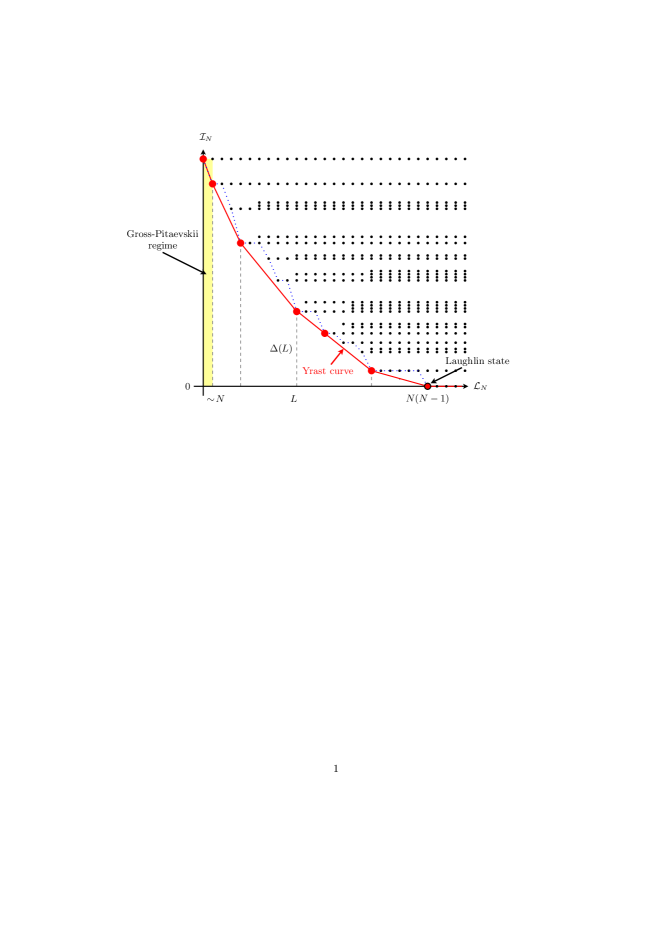
Figure 1: The joint spectrum of $\mathcal{L}_{N}$ and $\mathcal{I}_{N}$ (adapted from Lewin & Seiringer (2009)).

4.2.2 The uncorrelated (Gross-Piaevskii) regime

A rough estimate for the radius $R$ of the system, assuming that the kinetic and interaction energy of (29) are of the same order of magnitude, gives

$$R\sim(Ng/\omega)^{1/4}\qquad\hbox{\rm and}\qquad L\sim N\Omega R^{2}\sim N(Ng/\omega)^{1/2}.$$ (37)

Thus, if If $\omega/g\gg N^{-1}$ then $L\ll N^{2}$ and $\nu\gg 1$. In this case the ground state can be shown to be well described by an uncorrelated product state $\left(\varphi^{\rm GP}\right)^{\otimes N}$ where $N^{1/2}\varphi^{\rm GP}$ minimizes the Gross-Piitaevskii energy functional on Bargmann space (Aftalion et al (2006); Aftalion & Blanc (2008))

$$\mathcal{E}^{\rm GP}[\varphi]=\omega\langle\varphi,\mathcal{L}\varphi\rangle+\frac{g}{2}\int_{\mathbb{C}}|\varphi(z)|^{4}\exp(-2|z|^{2})\,\mathrm{d}^{2}z$$ (38)

under the condition $\int|\varphi|^{2}\exp(-|z|^{2})\mathrm{d}^{2}z=N$ with energy

$$E^{\rm GP}_{N}(\omega,g)=NE_{1}^{\rm GP}(\omega,Ng).$$ (39)

More precisely, the following holds (Lieb et al (2009)):

Theorem 1 (GP limit theorem in LLL).

For every $c>0$ there is a $C<\infty$ such that

$$E^{\rm GP}_{N}(\omega,g)\geq E_{N}(\omega,g)\geq E_{N}^{\rm GP}(\omega,g)(1-C(g/N\omega)^{1/10})$$ (40)

provided $gN/\omega>c$.

The lower bound covers the whole regime $L\ll N^{2}$, i.e., $\nu\gg 1$, but the GP description might have a wider range of applicability, see Fetter (2009) Section V C.

The proof of (1) uses similar techniques as in Lieb & Seiringer (2006) for the 3D GP limit theorem at fixed $\Omega$ and $Na$, in particular coherent states.

The analysis of the GP problem defined above is of interest in its own right Aftalion & Blanc (2008); Aftalion et al (2006); Gérard et al (2019). It is expected (see Aftalion (2006); Viefers (2008); Cooper (2008); Fetter (2009) and references therein) that for $\omega\to 0$ a vortex lattice is nucleated in the condensate. Namely, the zeroes of the analytic part of the GP minimizer in Bargmann space arrange on a triangular lattice in the bulk of the condensate, with a deformation at the edge Aftalion et al (2005); Ho (2001); Aftalion & Blanc (2008); Aftalion et al (2006). Taking this fact into consideration in a local density approximation, one expects that

$$E_{1}^{\rm GP}(\omega,Ng)\sim E^{\rm TF}(\omega,Ng)\mbox{ in the limit }\omega\to 0\mbox{ with }\omega\ll Ng\ll\omega^{-1}$$ (41)

where

$$E^{\rm TF}(\omega,Ng)=\min\left\{\int_{\mathbb{R}^{2}}\left(\left(\omega|x|^{2}-1\right)\rho(x)+\frac{Ng}{2}e^{\rm Ab}\rho(x)^{2}\right)dx\,|\,\rho\geq 0,\int\rho=1\right\}$$ (42)

with

$$e^{\rm Ab}\approx 1.16$$ (43)

the Abriskosov constant Abrikosov (1957); Aftalion et al (2006), i.e. the energy per area of a homogeneous vortex lattice. One also expects for the correspoing density of the GP minimizer

$$|u^{\rm GP}|^{2}\simeq\rho^{\rm TF}=\frac{1}{Nge^{\rm Ab}}\left(\lambda-\omega|x|^{2}\right)_{+}$$ (44)

in the same regime, where $\lambda$ is a chemical potential ensuring normalization. The above expectations were rigorously proven in Nguyen & Rougerie (2022) (under the restricted assumption that $Ng\ll\omega^{-3/5}$).

These results suggest a formula distribution of quantized vortices in the condensate. Indeed, writing the GP minimizer in the lowest Landau level in the manner

$$u^{\rm GP}(z)=c\prod_{j=1}^{m}(z-a_{j})e^{-\frac{|z|^{2}}{2}}$$ (45)

one finds Aftalion et al (2005); Ho (2001)

$$\sum_{j=1}^{m}\delta_{a_{j}}=\frac{1}{4\pi}\left(4+\Delta\log|u^{\rm GP}|^{2}\right)$$ (46)

for the empirical distribution of the zeroes of $u^{\rm GP}$, i.e., the locations of quantized vortices. Inserting the approximation (44) one finds

$$\sum_{j=1}^{m}\delta_{a_{j}}\simeq\frac{1}{\pi}+\frac{1}{4\pi}\Delta\log\left((\lambda-\omega|x|^{2})_{+}\right).$$ (47)

The first term, corresponding to a uniform density of vortices, dominates the asymptotics. The second one is a inhomogeneous correction, manifest mostly at the edge of the atomic cloud, see Aftalion et al (2005); Aftalion & Blanc (2008); Aftalion et al (2006) for more details.

The breakdown of the GP approximation is indicated by the number of vortices nucleated in the gas exceeding the total particle number. The above considerations indicate that this takes place when $g\gtrsim N\omega$, which marks the transition to a series of correlated many-body states, ending with a bosonic Laughlin function, as we discuss next.

4.3 Passage to the Laughlin state

As the filling factor decreases the ground state becomes increasingly correlated. The exact ground states are largely unknown (except for $L\leq N$ (Papenbrock & Bertsch (2001))), but candidates of states with various rational filling factors (composite fermion states, Moore-Read states, Read-Rezayi states,…) for energy upper bounds have been suggested and studied as discussed in the review article Cooper (2008).

If $\omega/g<\Delta/N^{2}$ one reaches the Laughlin state with filling factor $\frac{1}{2}$ whose wave function in Bargmann space is

$$\psi_{\rm Laughlin}(z_{1},\dots,z_{N})=c\prod_{i<j}(z_{i}-z_{j})^{2}.$$ (48)

It has interaction energy 0 and angular momentum $L=N(N-1)$. For an intuitive picture of the Laughlin state the following analogy may be helpful: The density $|\Psi_{\rm Laugh}(z_{1},...z_{N})|^{2}$ assigns probabilities to the possible configurations of $N$ points moving in the plane. The points like to keep a distance at least of order 1 from each other because the factors $|z_{i}-z_{j}|^{4}$ strongly reduce the probability when the particles are close. On the other hand the damping due to the gaussian favours a tight packing of the ‘balls’ of size $O(1)$ around the individual particles. The motion is strongly correlated in the sense that if one ball moves, all the other have also to move in order to satisfy these constraints.

5 Adding an anharmonic potential

The limit $\omega\to 0$, keeping $\omega>0$, is experimentally very delicate. For stability, but also to study new effects, we consider now a modification of the Hamiltonian (29) by adding a small anharmonic term:

$$H^{\rm LLL}_{N}\rightarrow H^{\rm LLL}_{k,N}:=H^{\rm LLL}_{N}+k\sum_{i=1}^{N}|z_{i}|^{4}$$ (49)

with a new parameter $k>0$. The potential $|z|^{4}$ can be expressed through $\mathcal{L}$ and $\mathcal{L}^{2}$ on Bargmann space, because with $\mathcal{L}=z\partial$ we have by partial integration, using the analyticity of $\varphi$:

$$\langle\varphi,\mathcal{L}\varphi\rangle=\int|{\varphi(z)}|^{2}(|z|^{2}-1)\exp(-|z|^{2})\,\mathrm{d}^{2}z$$ (50)

and

$$\langle\varphi,\mathcal{L}^{2}\varphi\rangle=\int(|z|^{4}-3|z|^{2}+1)|{\varphi(z)}|^{2}\exp(-|z|^{2})\,\mathrm{d}^{2}z.$$ (51)

Thus the modified Hamiltonian, denoted again by $H^{\rm 2D}_{N}$, can be written (up to an unimportant additive constant)

$$\boxed{H^{\rm LLL}_{k,N}=(\omega+{3k})\mathcal{L}_{N}+{k}\sum_{i=1}^{N}\mathcal{L}_{(i)}^{2}+g\,\mathcal{I}_{N}.}$$ (52)

5.1 Fully correlated states

The Bargmann space $\mathcal{B}^{N}$ with the scalar product (25) is naturally isomorphic to the Hilbert space $\mathcal{H}^{N}_{\rm LLL}\subset L^{2}(\mathbb{C})^{\otimes_{s}N},\mathrm{d}^{2N}z)$ consisting of wave functions of the form

$$\Psi(z_{1},\dots,z_{N})=\psi(z_{1},\dots,z_{N})\exp(-\sum_{j}|z_{j}|^{2}/2),\qquad\psi\in\mathcal{B}_{N}$$ (53)

with the standard $L^{2}$ scalar product. The energy can accordingly be considered as a functional on this space,

$$\mathcal{E}[\Psi]=\int V_{\omega,k}(z)\rho_{\Psi}^{(1)}(z)+\langle\Psi,\mathcal{I}_{N}\Psi\rangle,$$ (54)

where $\rho_{\Psi}^{(1)}$ is the one-particle density of $\Psi\in\mathcal{H}^{N}_{\rm LLL}$ with the normalization $\int\rho_{\Psi}^{(1)}(z)\,\mathrm{d}^{2}z=N$ and the potential is

$$V_{\omega,k}(z)=\omega\,|z|^{2}+k\,|z|^{4}.$$ (55)

Note that now $\omega<0$ is allowed, provided $k>0$.

We shall call states with vanishing interaction energy, i.e., $\Psi\in\mathrm{ker}\,\mathcal{I}_{N}$ fully correlated, because the particles stay away from each other in the sense that the wave function vanishes if $z_{i}=z_{j}$ for some pair $i\neq j$, in sharp contrast to a fully uncorrelated Hartree state. The fully correlated states in $\mathcal{H}^{N}_{\rm LLL}$ are of the form

$$\Psi(z_{1},...z_{N})=\phi(z_{1},\dots,z_{N})\Psi_{\rm Laugh}(z_{1},...z_{N})$$ (56)

with $\phi$ symmetric and analytic, and the Laughlin state

$$\Psi_{\rm Laugh}(z_{1},...z_{N})=c\prod_{i<j}\left(z_{i}-z_{j}\right)^{2}e^{-\sum_{j=1}^{N}|z_{j}|^{2}/2}.$$ (57)

For the Hamiltonian without the anharmonic addition to the potential the Laughlin state is an exact fully correlated ground state with energy 0 and angular momentum $L_{\rm Laugh}=N(N-1)$. This is not true for $k\neq 0$ because $\sum_{i=1}^{N}\mathcal{L}_{(i)}^{2}$ does not commute with $\mathcal{I}_{N}$. Note, however, that $\mathcal{L}_{N}$ still commutes with the Hamiltonian.

We now address the following question: Under what conditions is it possible to tune the parameters $\omega$, $g$ and $k$ so that a ground state $\Psi_{0}$ of (52) becomes fully correlated for $N\to\infty$? The following theorem, proved in Rougerie et al (2013) (see also Rougerie et al (2014)), gives sufficient conditions for this to happen. In order to state it as simply as possible we shall assume the ‘spectral gap conjecture’ of Subsection 4.2.1. This conjecture is not really needed, however, because is possible to replace the assumed universal gap $\Delta$ by other gaps depending on $N$, $\omega$ and $k$, cf. Eq. (IV.5) in Rougerie et al (2013).

Theorem 2 (Criteria for full correlation).

With $P_{({\rm Ker\,}\mathcal{I}_{N})^{\perp}}$ the projector onto the orthogonal complement of ${\rm Ker\,}\mathcal{I}_{N}$ we have

$$\left\|P_{({\rm Ker\,}\mathcal{I}_{N})^{\perp}}\Psi_{0}\right\|\to 0$$ (58)

in the limit $N\to\infty$, $\omega,k\to 0$ if one of the following conditions holds:

• $\omega\geq 0$ and $\omega N^{2}+kN^{3}\ll g\>\Delta$.

• $0\geq\omega\geq-2kN$ and $N(\omega^{2}/{k})+\omega N^{2}+kN^{3}\ll g\>\Delta$.

• $\omega\leq-2kN$, $|\omega|/k\lesssim N^{2}$ and $kN^{3}\ll g\>\Delta$

• $\omega\leq-2kN$, $|\omega|/k\gg N^{2}$ and $|\omega|N\ll g\>\Delta$

Note: For $k=0$ the first item is just the sufficient condition for the passage to the Laughlin state, $\omega/g<\Delta/N^{2}$, while the other conditions are void because $\omega<0$ is only allowed if $k>0$.

A proof of the Theorem is given in Section V of Rougerie et al (2013). It is based on two estimates:

• A lower bound for the ground state energy at fixed angular momentum $L$:

  $$E_{0}(L)\geq(\omega+3k)L+k\frac{L^{2}}{N}.$$ (59)

• An upper bound for the energy of suitable trial functions.

The first bound (59) is quite simple; it follows essentially from the inequality

$$\sum_{i}\mathcal{L}_{(i)}^{2}\geq\frac{1}{N}\left(\sum_{i}\mathcal{L}_{(i)}\right)^{2}$$ (60)

that holds because $\mathcal{L}_{(i)}$ and $\mathcal{L}_{(j)}$ commute for any $i,j$.

The upper bound is achieved by means of trial states of the form ‘giant vortex times Laughlin’, namely, with $m\geq 0$ and $c_{m,N}$ a normalization constant,

$$\Psi_{\rm gv}^{(m)}(z_{1},\dots,z_{N})=c_{m,N}\prod_{j=1}^{N}z_{j}^{m}\prod_{i<j}\left(z_{i}-z_{j}\right)^{2}e^{-\sum_{j=1}^{N}|z_{j}|^{2}/2}$$ (61)

These are special ‘quasi hole’ states (Laughlin (1983)) but for $m\gtrsim N$, i.e., $mN\gtrsim N^{2}$, the label ‘giant vortex’ appears more appropriate.

The energy of a trial state of the form (61) can be estimated using properties of the angular momentum operators and the radial symmetry in each variable of the gaussian measure with the pre-factor $\prod_{j=1}^{N}|z_{j}|^{2m}$. The computation is presented in Eqs. (V3)-(V7) in Rougerie et al (2013). Optimizing the estimate over $m$ leads to

$$m_{\rm opt}=\begin{cases}0&\mbox{\rm if }\omega\geq-2kN\\ \frac{|\omega|}{2k}-N&\mbox{\rm if }\omega<-2kN.\end{cases}$$ (62)

This is consistent with the picture that the Laughlin state is an approximate ground state in the first two cases of Theorem 1, in particular for negative $\omega$ as long as $|\omega|/k\lesssim N$. The angular momentum remains $O(N^{2})$ in these cases.

When $\omega<0$ and $|\omega|/(kN)$ becomes large the angular momentum is approximately

$$L_{\rm qh}:=N|\omega|/k\gg N^{2},$$ (63)

much larger than for the Laughlin state. A further transition at $|\omega|/k\sim N^{2}$ is manifest through the change of the subleading contribution to the energy of the trial functions. Its order of magnitude changes from $O(kN^{3})$ to $O(|\omega|N)$ at the transition.

To gain further insights into the physics of the transition we consider the particle density of the trial wave functions. This analysis (Rougerie et al (2014)) is based on Laughlin’s ‘plasma analogy’  where the $N$-particle density is written as a Gibbs distribution of a 2D Coulomb gas Laughlin (1983). This distribution can be studied in a rigorous mean field limit which brings out the essential features of the single particle density for large $N$.

5.2 The $N$-particle Density as a Gibbs Measure

We denote $(z_{1},\dots,z_{N})$ by $Z$ for short and consider the scaled $N$ particle density (normalized to 1)

$$\rho_{N,m}(Z):=N^{N}\left|\Psi_{\rm gv}^{(m)}(\sqrt{N}Z)\right|^{2}.$$ (64)

We can write

$$\hskip-2.84544pt\rho_{N,m}(Z) = \mathcal{Z}_{N,m}^{-1}\exp\left(\sum_{j=1}^{N}\left(-N|z_{j}|^{2}+2m\log|z_{j}|\right)+4\sum_{i<j}\log|z_{i}-z_{j}|\right)$$

$$= \mathcal{Z}_{N,m}^{-1}\exp\left(-\frac{1}{T}\mathcal{H}_{N,m}(Z)\right),$$

with $T=N^{-1}$ and

$$\mathcal{H}_{N,m}(Z)=\sum_{j=1}^{N}\left(|z_{j}|^{2}-\frac{2m}{N}\log|z_{j}|\right)-\frac{4}{N}\sum_{i<j}\log|z_{i}-z_{j}|.$$ (65)

5.2.1 Plasma analogy and mean field limit

The Hamilton function $\mathcal{H}_{N,m}(Z)$ is that of a classical 2D Coulomb gas (‘plasma’, one-component ‘jellium’) in a uniform background of opposite charge and with a point charge $(2m/N)$ at the origin, corresponding respectively to the $|z_{i}|^{2}$ and the $-\frac{2m}{N}\log|z_{j}|$ terms.

The probability measure $\rho_{N,m}(Z)$ minimizes the free energy functional

$$\mathcal{F}(\rho)=\int_{\mathbb{R}^{2N}}\mathcal{H}_{N,m}(Z)\rho(Z)+T\int_{\mathbb{R}^{2N}}\rho(Z)\log\rho(Z)$$ (66)

for this Hamiltonian at $T=N^{-1}$.

The $N\to\infty$ limit is in this interpretation a mean field limit where at the same time $T\to 0$. It is thus not unreasonable to expect that for large $N$, and in an appropriate sense,

$$\rho_{N,m}\approx\rho^{\otimes N}$$ (67)

with a one-particle density $\rho$ minimizing a mean field free energy functional.

The mean field free energy functional is defined as

$$\mathcal{E}^{\rm MF}_{N,m}[\rho]:=\int_{\mathbb{R}^{2}}W_{m}\,\rho-2\int_{\mathbb{R}^{2}}\int_{\mathbb{R}^{2}}\rho(z)\log|z-z^{\prime}|\rho(z^{\prime})+N^{-1}\int_{\mathbb{R}^{2}}\rho\log\rho$$ (68)

with

$$W_{m}(z)=|z|^{2}-2\frac{m}{N}\log|z|.$$ (69)

It has a minimizer $\rho^{\rm MF}_{N,m}$ among probability measures on $\mathbb{R}^{2}$ and this minimizer is in (Rougerie et al (2014)) proved to be a good approximation for the scaled 1-particle density of the trial wave function, i.e., for

$$\rho_{N,m}^{(1)}(z):=\int_{\mathbb{R}^{2(N-1)}}\rho_{N,m}(z,z_{2},\ldots,z_{N})\mathrm{d}^{2}z_{2}\ldots\mathrm{d}^{2}z_{N}.$$

(Recall the scaling: This density in the scaled variables $z$ is normalizes so that its integral is 1. The corresponding density in the physical, unscaled variables $\zeta=\sqrt{N}z$ has total mass $N$.)

5.2.2 Formulas for the mean field density

The picture of the 1-particle density that arises from asymptotic formulas for the mean-field density, valid for large $N$, is as follows:

If $m\leq N^{2}$, then $\rho^{\rm MF}_{m}$ is well approximated by a density $\hat{\rho}^{\rm MF}_{m}$ that minimizes the mean field functional without the entropy term $N^{-1}\int_{\mathbb{R}^{2}}\rho\log\rho$. This density takes a constant value $(2\pi)^{-1}$ on an annulus with inner and outer radii (in the scaled variables!)

$$R_{-}=(m/N)^{1/2},\qquad R_{+}=(2+m/N)^{1/2}$$

and is zero otherwise. The constant value is a manifestation of the incompressibility of the density of the trial state.

For $m\gtrsim N^{2}$ the entropy term becomes important and may dominate the electrostatic interaction term $\int\int\rho(z)\log|z-z^{\prime}|\rho(z^{\prime})$. The density is well approximated by a gaussian profile $\rho^{\rm th}(z)\sim|z|^{2m}\exp(-N|z|^{2})$ that is centered around $(m/N)^{-1/2}$ but has maximal value $\sim N/m^{1/2}\ll 1$ for $m\gg N^{2}$.

Thus, as the parameters $\omega$ and $k$ tend to zero and $N$ is large, the qualitative properties of the optimal trial wave functions exhibit different phases:

• For positive $\omega$, more generally for $\omega/k>-2N$, the Laughlin state is the ground state.

• When $\omega$ is negative and $|\omega|$ exceeds $2kN$ the state changes from a pure Laughlin state to a modified Laughlin state with a ‘hole’ in the density around the center.

• A further transition is indicated at $|\omega|\sim kN^{2}$. The density profile changes from being ‘flat’ to a Gaussian.

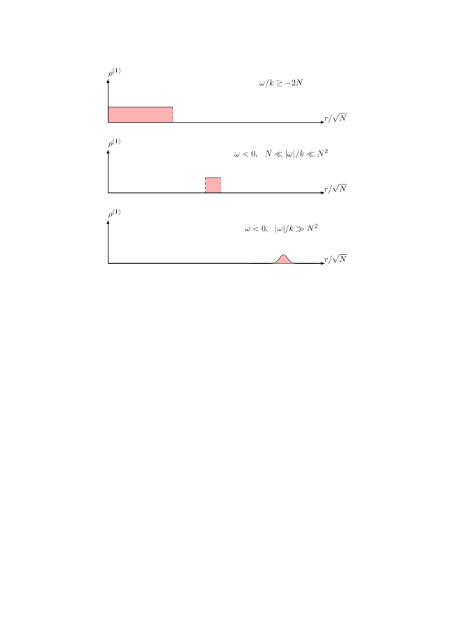
Figure 2: The three phases of the density $\rho^{(1)}_{N,m}$ (not to scale).

An intuitive understanding of these transitions may be obtained by employing the previous picture of the points $z_{i}$ as being the centers of essentially non overlapping balls of size $O(1)$. From the point of view of the plasma analogy the particles stay away from each other because of the repulsive Coulomb potential between them, while the attractive external potential due to the uniformly charged background keeps them as close together as possible. Modifying the wave function by a factor $\prod_{j}z_{j}^{m}$ has the effect of a repulsive charge of magnitude $m$ at the origin that pushes the particles (collectively!) away from the origin, creating a ‘hole’. The effect of such a hole on the energy of the wave function in the trap potential is to increase the energy if $\omega$ is positive. Hence the ground state will not have a hole. If $\omega<0$ the effective trapping potential has a Mexican hat shape with a minimum away from the origin, but since no ball can move without ‘pushing’ all the other balls, it is too costly for the system to take advantage of this as long as $k$ stays above the critical value $|\omega|/2N$. For smaller $k$ a hole is formed. The balls remain densely packed until the minimum of the Mexican hat potential moves so far from the origin that an annulus of width $O(1)$ at the radius of the minimum can accommodate all $N$ balls. This happens for $k\lesssim|\omega|/N^{2}$. For smaller $k$ (larger radius) the balls need not be tightly packed in the annulus and the average local density decreases accordingly.

5.3 Summary and Conclusions

The main conclusion from the analysis presented above of the ground states in the lowest Landau level generated by rapid rotation can be summarized as follows:

• For the Hamiltonan (29) the parameter regime $g\ll N\omega$, i.e., $L\ll N^{2}$, can be described by Gross-Piaevskii theory in the LLL.

• To enter the ‘fully correlated’ regime with $L\geq N(N-1)$ we have studied the Hamiltonian (52) with a quadratic plus quartic trap where the rotational frequency can exceed the frequency of the quadratic part of the trap, i.e, the frequency difference $\omega$ can be negative.

• Through the analysis of trial states for energy upper bounds, and simple lower bounds, we have obtained criteria for the ground state to be fully correlated in an asymptotic limit. The lower bounds, although not sharp, are of the same order of magnitude as the upper bounds.

• The particle density of the trial wave functions can be analyzed using Laughlin’s plasma analogy combined with rigorous mean field limits. The character of the ground state density changes at $|\omega|/k=O(N)$ and again at $|\omega|/k=O(N^{2})$.

Acknowledgments. Funding from the European Research Council (ERC) under the European Union’s Horizon 2020 Research and Innovation Programme (Grant agreement CORFRONMAT No 758620) is gratefully acknowledged.

References

- Abrikosov (1957) Abrikosov, A. A., 1957. The magnetic properties of superconducting alloys, J. Phys. Chem. Solids 2, pp. 199 - 208.
- Aftalion (2006) Aftalion, A., 2006. Vortices in Bose-Einstein Condensates, Progress in Nonlinear Differential Equations and their Applications 67, Birkhäuser, Basel.
- Aftalion & Blanc (2008) Aftalion A., Blanc X., 2006. Vortex Lattices in Rotating Bose–Einstein Condensates. SIAM Journal on Mathematical Analysis 38, pp. 874–893.
- Aftalion & Blanc (2008) Aftalion A., Blanc X., 2008. Reduced Energy Functionals for a Three Dimensional Fast Rotating Bose-Einstein Condensate. Ann. Inst. H. Poincaré C: Anal. Non Linéaire 25, pp. 339–355.
- Aftalion et al (2005) Aftalion, A., Blanc, X., Dalibard, J., 2005. Vortex patterns in a fast rotating Bose-Einstein condensate. Phys. Rev. A. 71, 023611.
- Aftalion et al (2006) Aftalion, A., Blanc, X., Nier, F., 2006. Lowest Landau Level Functionals and Bargmann Spaces for Bose-Einstein Condensates. J. Funct. Anal. 241, pp 661–702.
- Bargmann (1961) Bargmann, V., 1961. On a Hilbert space of analytic functions and an associated integral transform. Comm. Pure and Appl. Math., 14, pp. 187-214.
- Bretin et al (2004) Bretin,V., Stock, S., Seurin, Y., Dalibard, J., 2004. Fast Rotation of a Bose-Einstein Condensate. Phys. Rev. Lett. 92, 050403.
- Chakraborty & Pietiläinen (1988) Chakraborty, T., Pietiläinen, P., 1988. The Fractional Quantum Hall Effect. Springer, New York.
- Chakraborty & Pietiläinen (1995) Chakraborty, T., Pietiläinen, P., 1995. The Quantum Hall Effects, 2nd ed. Springer, New York.
- Ciftja (2006) Ciftja, O., 2006. Monte Carlo study of Bose Laughlin wave function for filling factors 1/2, 1/4 and 1/6. Europhys. Lett. 74, pp. 486-492.
- Clark et al (2020) Clark, L.W., Schine, N., Baum, C., Jia, N., Simon, J., 2020. Observation of Laughlin states made of light. Nature, 582, pp. 41-45.
- Cooper (2008) Cooper, N.R., 2008. Rapidly rotating atomic gases. Adv. in Phys., 57, pp. 539–616.
- Cornish et al (2000) Cornish, S.L., Claussen, N.R., Roberts, J.L., Cornell, E.A., Wieman, C.E., 2000. Stable Bose-Einstein Condensates with Widely Tunable Interactions. Phys. Rev. Lett. 85, pp. 1795–98.
- Correggi et al (2011) Correggi, M., Pinsker, F., Rougerie, N., Yngvason, J., 2011. Rotating superfluids in anharmonic traps: From vortex lattices to giant vortices. Phys. Rev. A 84, 053614
- Dalibard et al (2011) Dalibard, J., Gerbier F., Juzeliūnas G., Öhberg P., 2011.Artificial gauge potentials for neutral atoms. Rev. Mod. Phys. 83, 1523.
- Fetter (2009) Fetter, A.L., 2009. Rotating Trapped Bose-Einstein Condensates. Rev. Mod. Phys. 81, pp 647–691.
- Gérard et al (2019) Gérard, P., Germain, P., Thomann, L., 2019. On the cubic Lowest Landau Level equation. Arch. Ration. Mech. Anal. 231, pp 1073–1128.
- Girvin & Jach (1984) Girvin, S., Jach, T., 1984. Formalism for the quantum Hall effect: Hilbert space of analytic functions. Phys. Rev. B 29, pp. 5617–5625.
- Hauke & Carusotto (2022) Hauke, P., Carusotto I., 2022. Quantum Hall and Synthetic Magnetic-Field Effects in Ultra-Cold Atomic Systems. Encyclopedia of Condensed Matter Physics, 2nd edition. Elsevier.
- Ho (2001) Ho, T. L., 2001. Bose-Einstein condensates with large number of vortices. Phys. Rev. Lett. 87, 060403.
- Jain (2007) Jain, J. K., 2007. Composite fermions. Cambridge University Press.
- Ketterle et al (1996) Ketterle, W., van Druten, N.J., 1996. Evaporative Cooling of Trapped Atoms. Advances in Atomic, Molecular and Optical Physics 37, pp. 181–236. Academic Press.
- Laughlin (1983) Laughlin, R. B., 1983. Anomalous quantum Hall effect: An incompressible quantum fluid with fractionally charged excitations. Phys. Rev. Lett. 50, pp. 1395–1398.
- Lewin & Seiringer (2009) Lewin, M., Seiringer, R., 2009. Strongly Correlated Phases in Rapidly Rotating Bose Gases. J. Stat. Phys. 137, pp. 1040–1062.
- Lieb et al (2016) Lieb, E. H., Rougerie, N., Yngvason, J., 2018. Rigidity of the Laughlin liquid. J. Stat. Phys. 172, pp. 544–554.
- Lieb & Seiringer (2006) Lieb E.H., Seiringer, R., 2006. Derivation of the Gross-Pitaevskii Equation for Rotating Bose Gases. Commun. Math. Phys. 264, pp. 505-537.
- Lieb et al (2009) Lieb E.H., Seiringer, R., Yngvason J., 2009. The yrast Line of a Rapidly Rotating Bose Gas: The Gross-Pitaevskii Regime. Phys. Rev. A 79, 063626.
- Nachtergaele et al (2020) Nachtergaele, B., Warzel, S., Young, A., 2020. Low-complexity eigenstates of a fractional quantum Hall system. Journal of Physics A: Mathematical and Theoretical, 1. p. 01LT01.
- Nguyen & Rougerie (2022) Nguyen, D.-Th., Rougerie, N., 2022. Thomas-Fermi profile of a fast rotating Bose-Einstein condensate. Pure and Applied Analysis, to appear. ArXiv:2201.04418.
- Papenbrock & Bertsch (2001) Papenbrock, T., Bertsch, G.F., 2001. Rotational spectra of weakly interacting Bose-Einstein condensates. Phys. Rev. A 63, 023616.
- Pethick & Smith (2008) Pethick, C., Smith, H., 2008. Bose-Einstein Condensation of Dilute Gases, 2nd edition, Cambridge University Press.
- Pitaevskii & Stringari (2016) Pitaevskii L., Stringari S., 2016. Bose-Einstein Condensation, 2nd edition, Oxford Science Publications, Oxford.
- Prange & Girvin (1987) Prange, R. E., Girvin, S. E., eds., 1987. The quantum Hall effect. Springer.
- Regnault et al (2006) Regnault, N.,Chang, C.C., Jolicoeur, Th, Jain, J.K., 2006. Composite fermion theory of rapidly rotating two-dimensional bosons, 2006. J. Phys. B: At. Mol. Opt. Phys. 39. S89-S99
- Roncaglia et al (2011) Roncaglia, M., Rizzi, M., Dalibard, J., 2011. From Rotating Atomic Rings to Quantum Hall States. Sci. Rep. 1, pp 43.
- Rougerie et al (2014) Rougerie, N., Serfaty, S., Yngvason, J., 2014. Quantum Hall phases and plasma analogy in rotating trapped Bose gases. J. Stat. Phys. 154,
- Rougerie et al (2013) Rougerie, N., Serfaty, S., Yngvason, J. 2013. Quantum Hall phases and plasma analogy in rotating trapped Bose gases. Phys. Rev. A 87, 023618.
- Schweikhard et al (2004) Schweikhard,V., Coddington, I., Engels,P., Mogendorff, V.P., Cornell, E.A., 2004. Rapidly Rotating Bose-Einstein Condensates in and near the Lowest Landau Level. Phys. Rev. Lett. 92, 040404.
- Seiringer & Yngvason (2020) Seiringer, R., Yngvason, J., 2020. Emergence of Haldane Pseudo-potentials in Systems with Short Range Interactions. J. Stat. Phys. 281, pp. 448–464.
- Störmer et al (1999) Störmer, H.L., Tsui, D.C., Gossard, A.C., 1999. The fractional quantum Hall effect. Rev. Mod. Phys. 71, pp. S298–S305.
- Viefers et al (2000) Viefers, S., Hansson, T. H., Reimann, S. M., 2000. Bose condensates at high angular momenta. Phys. Rev. A 62, 053604.
- Viefers (2008) Viefers, S., 2008. Quantum Hall physics in rotating Bose-Einstein condensates. J. Phys. C 12, p. 123202.
- Warzel & Young (2021a) Warzel. S., Young, A., 2021. The spectral gap of a fractional quantum Hall system on a thin torus. ArXiv:2112.13764.
- Warzel & Young (2021b) Warzel. S., Young, A., 2021. A bulk spectral gap in the presence of edge states for a truncated pseudopotential. ArXiv:2108.10794.