Optical circular polarization induced by axionlike particles in blazars

Abstract

We propose that the interaction between the axionlike particles (ALPs) and photons can be a possible origin of optical circular polarization (CP) in blazars. Given that there is no definite detection of optical CP at $\sim 0.1\%$ level, a rough limit on ALP-photon coupling can be obtained, specifically $g_{a\gamma}\cdot B_{\mathrm{T0}}\lesssim 7.9\times 10^{-12}~{}\mathrm{G\cdot GeV}^{-1}$ for $m_{a}\lesssim 10^{-13}~{}\mathrm{eV}$, depending on the magnetic field configuration of the blazar jet. Obviously, for the blazar models with a larger magnetic field strength, such as hadronic radiation models, this constraint could be more stringent. We also perform a dedicated analysis of the tentative observations of optical CP in two blazars, namely 3C 66A and OJ 287, and we find that these observations could be explained by the ALP-photon mixing with $g_{a\gamma}\sim 10^{-11}~{}\mathrm{GeV}^{-1}$. As an outlook, our analysis can be improved by further research on the radiation models of blazars and high-precision joint measurements of optical CP and linear polarization.

I Introduction

Axionlike particles (ALPs) are very light pseudoscalar particles that appear in many extensions of the Standard Model (SM) Witten (1984); Svrcek and Witten (2006); Conlon (2006a, b); Arvanitaki et al. (2010); Acharya et al. (2010); Cicoli et al. (2012). These particles constitute a generalization of the quantum chromodynamics (QCD) axion, which is a pseudo-Goldstone boson arising from the Peccei-Quinn symmetry breaking mechanism and can be treated as an excellent solution to the strong CP problem Peccei and Quinn (1977a, b); Weinberg (1978); Wilczek (1978); Cheng (1988). Meanwhile, unlike the QCD axion, the coupling and mass of the ALP are, in principle, independent parameters, thus a much wider parameter space is spanned in the ALP scenario. ALPs are extremely appealing as they can also play important roles in cosmology and astrophysics Kolb and Turner (1990); Turner (1990); Sikivie (2008); Carroll (1998). For instance, ALPs are good candidates for dark matter Marsh (2016); Preskill et al. (1983); Abbott and Sikivie (1983); Dine and Fischler (1983).

At low energies, ALPs could interact with the SM particles through the effective operators that are suppressed by some high energy scales Graham et al. (2015). For example, ALPs may interact with the electromagnetic sector through the Lagrangian term $\mathcal{L}=g_{a\gamma}a\bm{E}\cdot\bm{B}$. This interaction can lead to two distinct effects in astrophysics, which provide promising ways to detect ALPs. One is the polarization rotation of photons as they propagate in a variable ALP background field, due to the change of the dispersion relation of the photons Fedderke et al. (2019); Schwarz et al. (2021); Ivanov et al. (2019); DeRocco and Hook (2018); Obata et al. (2018); Caputo et al. (2019); Chen et al. (2020); Yuan et al. (2021). The other is the ALP-photon conversion in the external magnetic field Sikivie (1983); Raffelt and Stodolsky (1988). The mixing occurs between the ALP and the photon polarization component that in parallel to the magnetic field. In particular, this process changes not only the amplitude but also the polarization of the photon Raffelt and Stodolsky (1988); Maiani et al. (1986). Considering that the ALP-photon coupling is particularly weak, many studies focus on the conversion for high energy photons Csaki et al. (2003); De Angelis et al. (2007); Hooper and Serpico (2007); Simet et al. (2008); Sanchez-Conde et al. (2009); Mirizzi and Montanino (2009); Bassan et al. (2010); De Angelis et al. (2011); Galanti et al. (2019); Dessert et al. (2020) or the resonant conversion in strong magnetic fields Pshirkov and Popov (2009); Hook et al. (2018); Huang et al. (2018); Dessert et al. (2019); Darling (2020); Edwards et al. (2021); Wang et al. (2021a, b); Prabhu (2021); Dessert et al. (2022). Otherwise, the magnetic fields in large scales, e.g., the supercluster at scale of $\sim 10~{}\mathrm{Mpc}$, are needed to achieve a significant conversion Jain et al. (2002); Agarwal et al. (2008); Payez et al. (2011, 2012); Tiwari (2017). In particular, the ALP-photon mixing in extragalactic magnetic fields is proposed to explain the dimming of type Ia supernovae Csaki et al. (2002); Grossman et al. (2002); Mirizzi et al. (2008); Avgoustidis et al. (2010); Liao et al. (2015); Buen-Abad et al. (2022).

Many studies have addressed the ALP effects on the observed spectrum and polarization state of $\gamma$-rays from sources like blazars in astrophysical magnetic fields Csaki et al. (2003); De Angelis et al. (2007); Hooper and Serpico (2007); Simet et al. (2008); Sanchez-Conde et al. (2009); Mirizzi and Montanino (2009); Bassan et al. (2010); De Angelis et al. (2011); Galanti et al. (2019); Meyer et al. (2014); Tavecchio et al. (2015); Day and Krippendorf (2018); Galanti (2022a, b); Galanti et al. (2022), including those in the blazar jet, galaxy cluster, intergalactic space, and Milky Way. However, the mixing effect is rarely discussed for low energy photons, especially within the source region of blazars. In fact, there are some advantages to study such effect. It is easier to measure the polarization of low energy photons with high precision Krawczynski et al. (2016); Soffitta (2017). Besides, with the multiwavelength observations of blazars, we have a better understanding of their properties, such as the radiation mechanism and the magnetic field structures Urry and Padovani (1995); Angel and Stockman (1980), which in turn helps us to understand the initial polarization state of photons. Based on these facts, it is an intriguing project to investigate the ALP effect on the optical photon polarization state from blazars.

It is expected that ALPs would not significantly change the flux and linear polarization (LP) of the optical photons from blazars. However, we find that under some suitable conditions, ultra-light ALPs can lead to an appreciable circular polarization (CP), which may be an origin of optical CP in blazars. Conversely, the ALPs can be explored through some tentative CP observations of blazars.

In recent years, several optical polarization monitoring programs have been carried out, and mainly focus on the linear polarization signature Zhang (2019). However, the optical circular polarization in blazars has rarely been searched for. This is partly because that optical CP is expected to be low in usual physical processes Rieger and Mannheim (2005), requiring very sensitive instruments to deliver CP measurements. If the ALP-photon mixing can lead to an appreciable CP for the optical photons from blazars, we appeal to implement more sensitive experiments that can simultaneously measure the optical LP and CP to further nail down the effects of ALPs.

The paper is organized as follows. In Sec. II, we present a brief calculation routine of the ALP-photon mixing and derive the CP formulas under the weak-mixing condition. In Sec. III, we introduce the jet configuration of BL Lac, which is a type of blazar, and obtain results using the CP formulas. In Sec. IV, we analyze the ALP effects in the tentative CP observations of two blazars. In Sec. V, we discuss several relevant factors that may affect the results. Conclusions are given in Sec. VI. Note that all equations are expressed in Lorentz–Heaviside units throughout the paper.

II ALP-photon mixing in magnetic fields

II.1 Mixing in one domain

The calculation routines used for the ALP-photon conversion have been described in detail in many papers, e.g., Mirizzi and Montanino (2009); Bassan et al. (2010); De Angelis et al. (2011); Meyer et al. (2014). Nevertheless, for the reader’s convenience, we briefly summarize all necessary elements here. The ALP-photon system can be described by the Lagrangian

$$\mathcal{L}_{\mathrm{ALP}} =\frac{1}{2}\partial^{\mu}a\partial_{\mu}a-\frac{1}{2}m_{a}^{2}a^{2}-\frac{1}{4}g_{a\gamma}aF_{\mu\nu}\tilde{F}^{\mu\nu}$$ (1)

$$=\frac{1}{2}\partial^{\mu}a\partial_{\mu}a-\frac{1}{2}m_{a}^{2}a^{2}+g_{a\gamma}a\bm{E}\cdot\bm{B},$$

where $a$ denotes the ALP field, $F_{\mu\nu}$ and $\tilde{F}^{\mu\nu}$ are the electromagnetic tensor and its dual, respectively. For the ALP, the mass $m_{a}$ is unrelated to its coupling with photons $g_{a\gamma}$. The ALP-photon mixing in the presence of an external magnetic field $\bm{B}$ is characterized by the $a\gamma\gamma$ vertex in the Lagrangian. Only the transverse component of the external magnetic field $\bm{B}_{\mathrm{T}}$ with respect to the direction of beam propagation matters.

We assume a monochromatic ALP-photon beam with energy of $E\gg m_{a}$ propagating in the $z$ direction. In the short-wavelength approximation, the equation of motion (EOM) can be written as Raffelt and Stodolsky (1988)

$$\left(i\frac{d}{dz}+E+\mathcal{M}\right)\psi(z)=0$$ (2)

with

$$\psi(z)=\left(\begin{array}[]{c}A_{x}(z)\\ A_{y}(z)\\ a(z)\end{array}\right),$$ (3)

where $A_{x}(z)$ and $A_{y}(z)$ denote the LP amplitudes of the photon along the x- and y-axis, respectively, and $a(z)$ is the ALP amplitude.

In analysis, the astrophysical magnetic field is often supposed to be homogeneous in a single small domain. If its transverse component $\bm{B}_{\mathrm{T}}$ is set along with the $y$-axis, the mixing matrix is given by Kuster et al. (2008)

$$\mathcal{M}^{(0)}=\left(\begin{array}[]{ccc}\Delta_{\perp}&0&0\\ 0&\Delta_{\parallel}&\Delta_{a\gamma}\\ 0&\Delta_{a\gamma}&\Delta_{a}\end{array}\right)~{},$$ (4)

with

$$\Delta_{a\gamma}\equiv\frac{1}{2}g_{a\gamma}B_{\mathrm{T}},$$ (5)

$$\Delta_{a}\equiv-\frac{m_{a}^{2}}{2E}.$$ (6)

$\Delta_{a\gamma}$ and $\Delta_{a}$ account for the ALP-photon mixing and ALP mass effect, respectively. Since we consider the photons in the optical band here, other off-diagonal $\Delta$-terms related to the Faraday rotation are neglected.

The diagonal terms related to the photon constitute four parts as Galanti and Roncadelli (2018); Davies et al. (2021)

$$\Delta_{\perp}\equiv\Delta_{\mathrm{pl}}+\Delta_{\mathrm{abs}}+\Delta_{\mathrm{CMB}}+2\Delta_{\mathrm{QED}},$$ (7)

$$\Delta_{\parallel}\equiv\Delta_{\mathrm{pl}}+\Delta_{\mathrm{abs}}+\Delta_{\mathrm{CMB}}+3.5\Delta_{\mathrm{QED}},$$ (8)

with

$$\Delta_{\mathrm{pl}}\equiv-\frac{\omega^{2}_{\mathrm{pl}}}{2E},$$ (9)

$$\Delta_{\mathrm{abs}}\equiv\frac{i}{2\lambda_{\gamma}},$$ (10)

$$\Delta_{\mathrm{CMB}}\equiv\chi_{\mathrm{CMB}}E,$$ (11)

$$\Delta_{\mathrm{QED}}\equiv\frac{\alpha E}{45\pi}\left(\frac{B_{\mathrm{T}}}{B_{\mathrm{cr}}}\right)^{2}.$$ (12)

$\Delta_{\mathrm{pl}}$ accounts for the effective photon mass when the beam propagates in the plasma with the frequency parameter $\omega_{\mathrm{pl}}=(4\pi\alpha n_{e}/m_{e})^{1/2}$, where $\alpha$ is the fine-structure constant, $n_{e}$ and $m_{e}$ denote the electron number density and the electron mass, respectively. The other three contributions, including $\Delta_{\mathrm{abs}}$ the photon absorption term with the mean free path $\lambda_{\gamma}$, $\Delta_{\mathrm{CMB}}$ the photon dispersion term induced by the cosmic microwave background with the refractive index $\chi_{\mathrm{CMB}}\simeq 0.522\times 10^{-42}$ Dobrynina et al. (2015), and $\Delta_{\mathrm{QED}}$ the QED vacuum polarization term with $B_{\mathrm{cr}}\simeq 4.4\times 10^{13}~{}\mathrm{G}$, are negligible in the scenario here. That is to say, we can safely make the approximation $\Delta_{\parallel}\approx\Delta_{\perp}\simeq\Delta_{\mathrm{pl}}$.

In a general situation, the transverse magnetic field $\bm{B}_{T}$ is not aligned with the y-axis. We denote $\phi$ the angle between $\bm{B}_{T}$ and the y-axis in a generic domain. Correspondingly, the mixing matrix can be obtained using the similarity transformation

$$\mathcal{M}=V^{\dagger}(\phi){\cal M}^{(0)}V(\phi)$$ (13)

operated by the rotation matrix in the $x$-$y$ plane, namely

$$V(\phi)=\left(\begin{array}[]{ccc}\cos\phi&-\sin\phi&0\\ \sin\phi&\cos\phi&0\\ 0&0&1\end{array}\right).$$ (14)

In view of our subsequent discussion, the polarization density matrix is introduced as

$$\rho(z)=\left(\begin{array}[]{c}A_{x}(z)\\ A_{y}(z)\\ a(z)\end{array}\right)\otimes\left(\begin{array}[]{c}A_{x}(z)\ A_{y}(z)\ a(z)\end{array}\right)^{*},$$ (15)

which obeys the Liouville-Von Neumann equation

$$i\frac{d\rho}{dz}=[\rho,\mathcal{M}].$$ (16)

The solution of Eq. (16) is

$$\rho(z)=\mathcal{T}(z,z_{0})\,\rho(z_{0})\,\mathcal{T}^{\dagger}(z,z_{0})~{},$$ (17)

where the transfer function $\mathcal{T}(z,z_{0})$ is the solution of the EOM in the form of $\psi(z)=\mathcal{T}(z,z_{0})\psi(z_{0})$ with the initial condition $\mathcal{T}(z_{0},z_{0})=1$. The probability that an ALP-photon beam initially in the state $\rho(z_{0})$ converts into the state $\rho_{\mathrm{f}}$ at a position with $z$ can be computed as

$$P=\mathrm{Tr}(\rho_{\mathrm{f}}\mathcal{T}(z,z_{0})\,\rho(z_{0})\,\mathcal{T}^{\dagger}(z,z_{0})).$$ (18)

For a fixed magnetic field, the probability that a photon polarized along the y-axis oscillates into an ALP after a distance $d$ can simply read

$$P_{\gamma\to a}=\cos^{2}\phi\sin^{2}(2\theta)\sin^{2}(\frac{\Delta_{\mathrm{osc}}d}{2}),$$ (19)

with the ALP-photon mixing angle

$$\theta=\frac{1}{2}\arctan(\frac{2\Delta_{a\gamma}}{\Delta_{\parallel}-\Delta_{a}})$$ (20)

and the oscillation wave number

$$\Delta_{\mathrm{osc}}=[(\Delta_{a}-\Delta_{\parallel})^{2}+4\Delta_{a\gamma}^{2}]^{1/2}.$$ (21)

As for the numerical calculation with a more realistic configuration of the astrophysical magnetic field, the field environment can be sliced into $N$ consecutive domains with homogeneous magnetic fields. For each domain, the EOM can be solved exactly. By iterating, we can derive the photon and/or axion state at any propagation distance.

II.2 Optical circular polarization

The $2\times 2$ density matrix of the photon polarization (i.e., the 2-2 block of the density matrix for the ALP-photon system) can be expressed in terms of the Stokes parameters Kosowsky (1996)

$$\rho_{\gamma}=\frac{1}{2}\left(\begin{array}[]{cc}I+Q&U-iV\\ U+iV&I-Q\\ \end{array}\right).$$ (22)

The degree of CP is defined as Rybicki (2004)

$$\Pi_{C}\equiv\frac{V}{I}.$$ (23)

In this study, we work within the weak-mixing condition, i.e.

$$\begin{gathered}|\Delta_{\mathrm{pl}}|\gg\Delta_{a\gamma},\\ |\Delta_{\mathrm{pl}}|\gg|\Delta_{a}|.\end{gathered}$$ (24)

In this regime, $\theta\ll 1$ and the conversion probability turns out to be vanishingly small. Expanding Eq. (17) and neglecting the high order terms, the evolution of the Stokes parameters in a single domain region can be obtained as

$$I(z)=I(z_{0})-\mathcal{I}(1-\cos\kappa),$$ (25)

$$Q(z)=Q(z_{0})-\mathcal{Q}_{1}(1-\cos\kappa)-\mathcal{Q}_{2}\sin\kappa,$$ (26)

$$U(z)=U(z_{0})-\mathcal{U}_{1}(1-\cos\kappa)-\mathcal{U}_{2}\sin\kappa,$$ (27)

$$V(z)=V(z_{0})\cos\kappa+\mathcal{V}\sin\kappa,$$ (28)

where

$$\mathcal{I}\equiv Q(z_{0})\sin^{2}2\phi,$$ (29)

$$\mathcal{Q}_{1}\equiv\frac{1}{2}U(z_{0})\sin 4\phi,$$ (30)

$$\mathcal{Q}_{2}\equiv V(z_{0})\sin 2\phi,$$ (31)

$$\mathcal{U}_{1}\equiv\left[Q(z_{0})\sin 2\phi+U(z_{0})\cos 2\phi\right]\cos 2\phi,$$ (32)

$$\mathcal{U}_{2}\equiv V(z_{0})\cos 2\phi,$$ (33)

$$\mathcal{V}\equiv Q(z_{0})\sin 2\phi+U(z_{0})\cos 2\phi,$$ (34)

$$\kappa\equiv\frac{\Delta_{a\gamma}^{2}}{\Delta_{\mathrm{pl}}-\Delta_{a}}(z-z_{0})~{}.$$ (35)

Supposing $|\kappa|\ll 1$ in each domain and the degree of CP of the incident beam can be neglected, the above equations show that the changes of $I$, $Q$, and $U$ are negligible at first leading order. For the CP, we can evaluate it across multidomains as

$$V(z)-V(z_{0})$$ (36)

$$\approx \int_{z_{0}}^{z}\mathcal{V}\frac{\Delta_{a\gamma}^{2}}{\Delta_{\mathrm{pl}}-\Delta_{a}}dz^{\prime}$$

$$= -\frac{m_{e}g_{a\gamma}^{2}\mathcal{V}E}{8\pi\alpha}\int_{z_{0}}^{z}\frac{B_{T}^{2}(z^{\prime})}{n_{e}(z^{\prime})}dz^{\prime}.$$

The parameter $\mathcal{V}$ is determined by the LP state of incident photons and the direction of the transverse magnetic field. For the above equation, we have made the assumption that the direction of transverse magnetic field remains unchanged, thus $\mathcal{V}$ can be treated as constant. A general polarization density matrix of a beam of linearly polarized photons can be written as

$$\begin{gathered}\rho_{\gamma}(\Pi_{\mathrm{L}},\psi)=\left(\begin{array}[]{cc}\frac{1-\Pi_{\mathrm{L}}\cos 2\psi}{2}&\frac{\Pi_{\mathrm{L}}\sin 2\psi}{2}\\ \frac{\Pi_{\mathrm{L}}\sin 2\psi}{2}&\frac{1+\Pi_{\mathrm{L}}\cos 2\psi}{2}\\ \end{array}\right),\end{gathered}$$ (37)

where

$$\Pi_{\mathrm{L}}\equiv\frac{\sqrt{Q^{2}+U^{2}}}{I}$$ (38)

is the degree of LP, and $\psi$ is the polarization angle relative to the y-axis. Then, Eq. (34) can be rewritten as

$$\mathcal{V}=\Pi_{\mathrm{L}}\sin 2(\phi-\psi).$$ (39)

The above equations show that the magnitude of the ALP induced CP is proportional to the LP degree of the photons in the weak-mixing regime. When $\phi-\psi$, which denotes the angle between the LP and the transverse magnetic field, equals $(2k+1)\pi/4$ with $k\in\mathbb{Z}$, $\mathcal{V}$ reaches the extreme value $\pm\Pi_{\mathrm{L}}$.

Even though the energy of the photon and the magnetic field strength may not be high, the integration indicates that the ALPs can induce a considerable CP as long as the field environment is suitable and the spatial scale of magnetic field is large enough. This makes blazars good candidate sources, as discussed in the next section.

III Application in blazars

Blazars are active galactic nuclei with a relativistic jet pointing very close to Earth Urry and Padovani (1995). The highly collimated and Doppler boosted jet make them bright and variable in all wavebands from the radio to $\gamma$-ray Angel and Stockman (1980). Blazars are categorized as BL Lac objects (BL Lacs) Shaw et al. (2013) and flat-spectrum radio quasars (FSRQs) Shaw et al. (2012), which were mostly called optically violent variable quasars. Compared to BL Lacs, FSRQs are generally more luminous and show broad emission lines in the optical and UV bands. The jet of BL Lacs could extend to $\sim\mathrm{kpc}$. In the jet the magnetic field is substantially ordered and predominantly traverse to the jet Pudritz et al. (2012).

The degree of optical LP in blazars is typically at a level of $\sim 10\%$ and can be up to $\sim 50\%$ sometimes, while no definite CP has been detectedHutsemekers et al. (2010); Zhang (2019). Therefore, we can set a constraint on the parameters of the ALP utilizing the effect discussed in the previous section. We focus on BL Lacs in the discussion below, considering that the field environment of FSRQs are more complicated and the geometry and intensity of $\bm{B}$ are less clear compared to BL Lacs Pudritz et al. (2012); Prandini and Ghisellini (2022).

III.1 Field configuration of BL Lacs

Faraday rotation measure (RM) is an important tool in astronomy, and enables one to study the magnetic field and electron number density of blazar jets. Many observations have detected the transverse RM gradients across the jets of BL Lacs, which evidence that these jets have the toroidal or helical magnetic fields Gabuzda et al. (2004, 2017); Kravchenko et al. (2017). The conservation of the Poynting flux demands that the magnetic field strength varies as $d^{-1}$, where $d$ is the transverse size of the jet Begelman et al. (1984); Rees (1987). The conservation of particles demands that the number density varies as $r^{-2}$ O’Sullivan and Gabuzda (2009), where $r$ is the distance from the source of the jet. In this work, we adopt the conical shaped model used in Meyer et al. (2014); Tavecchio et al. (2015). In the comoving frame, the transverse magnetic field and electron density of the jet are modeled by

$$B_{T}^{\mathrm{jet}}=B_{T0}\left(\frac{r}{r_{\mathrm{E}}}\right)^{-1}$$ (40)

and

$$n_{e}^{\mathrm{jet}}=n_{e0}\left(\frac{r}{r_{\mathrm{E}}}\right)^{-2}$$ (41)

for $r>r_{\mathrm{E}}$, where $r_{\mathrm{E}}$ is the distance of the emission site from the central black hole. The value of $r_{\mathrm{E}}$ is usually inferred from the size of the emission region and the jet aperture angle, typically ranging from $0.01~{}\mathrm{pc}$ to $0.1~{}\mathrm{pc}$ Celotti and Ghisellini (2008). However, it will be found in the latter discussion that the value of $r_{\mathrm{E}}$ has little effect on our results, thus we choose $r_{\mathrm{E}}=0.05~{}\mathrm{pc}$ in order to be definite. For the electron density at the emission site $n_{\mathrm{e0}}$ and the size of the jet $r_{\mathrm{max}}$, the typical values are $n_{\mathrm{e0}}\simeq 5\times 10^{4}~{}\mathrm{cm}^{-3}$ and $r_{\mathrm{max}}\simeq 1~{}\mathrm{kpc}$ Meyer et al. (2014); Tavecchio et al. (2015). The exact value of $n_{\mathrm{e0}}$ for the specific blazar is not definite in general, however it can be inferred from fitting parameters of the spectral energy distributions (SEDs) of blazars.

The SEDs of blazars are dominated by two distinct radiative components: a broad low-frequency component from radio to optical/UV or x-ray and a high-frequency component from x-ray to $\gamma$-ray. It is generally accepted that the low-frequency component is produced by the synchrotron radiation of relativistic electrons in the jets. For the interpretation of the high-frequency component, synchrotron self-Compton (SSC) and external Compton (EC) are two main mechanisms. Hence, the popular models differ by the radiation particles into two kinds, namely leptonic (emission dominated by electrons and possibly positrons) and hadronic (emission dominated by protons) models Blandford et al. (2019); Prandini and Ghisellini (2022). In the leptonic models, the SED fitting usually gives a magnetic field strength of $0.1-1~{}\mathrm{G}$ for Intermediate BL Lacs and $1-3~{}\mathrm{G}$ for Low-Frequency-Peaked BL Lacs Boettcher et al. (2013). However, in the hadronic models, the magnetic field strength is much lager, ranging from $10~{}\mathrm{G}$ to $100~{}\mathrm{G}$ Boettcher et al. (2013). For the convenience of study, we choose the typical parameter $B_{T0}\simeq 1~{}\mathrm{G}$. The different results can be inferred depending on the radiation models of blazars.

The current most robust bound on $g_{a\gamma}$ in the parameter region of interest here is provided by the CAST experiment, which constrains $g_{a\gamma}<6.6\times 10^{-11}~{}\mathrm{GeV}^{-1}$ for $m_{a}<0.02~{}\mathrm{eV}$ Anastassopoulos et al. (2017). Other studies can also set stronger constraints depending on specific procedures (e.g., Grifols et al. (1996); Payez et al. (2015); Berg et al. (2017); Marsh et al. (2017)). In this work, we choose $g_{a\gamma}=5\times 10^{-11}~{}\mathrm{GeV}^{-1}$ allowed by the CAST bound as the benchmark value.

In the rest of this subsection, we discuss the validity of the weak-mixing condition. The first condition of Eq. (24) requires

$$\left(\frac{g_{a\gamma}}{5\times 10^{-11}\mathrm{GeV}^{-1}}\right)\left(\frac{E}{\mathrm{1eV}}\right)\ll 1.45\left(\frac{B_{T}}{1\mathrm{G}}\right)^{-1}\left(\frac{n_{e}}{1\mathrm{cm}^{-3}}\right).$$ (42)

In the case of blazar, this means that the weak-mixing condition is satisfied for

$$r\ll 28~{}\mathrm{kpc}\left(\frac{B_{T0}}{1~{}\mathrm{G}}\right)^{-1}\left(\frac{n_{e0}}{5\times 10^{4}~{}\mathrm{cm}^{-3}}\right)\left(\frac{r_{\mathrm{E}}}{0.05~{}\mathrm{pc}}\right)\left(\frac{g_{a\gamma}}{5\times 10^{-11}~{}\mathrm{GeV}^{-1}}\right)^{-1}\left(\frac{E^{\prime}}{2~{}\mathrm{eV}}\right)^{-1}\left(\frac{\delta}{15.64}\right).$$ (43)

where $\delta$ is the relativistic Doppler factor and $E^{\prime}$ is the energy of photons in the rest frame. The photon energy $E$ in the co-moving frame is related to the observed energy $E^{\prime}$ through the Doppler factor $\delta$ as $E=E^{\prime}/\delta$. The observed energy $E^{\prime}\simeq 2~{}\mathrm{eV}$ corresponds to the photons in the optical waveband, and $\delta=15.64$ is taken to be the same typical value as Meyer et al. (2014). Straightforwardly, the more stringent constraint on $g_{a\gamma}$ is required for the larger magnetic field strength to meet the condition above.

The second condition of Eq. (24) requires the mass of the ALP and the size of the jet

$$m_{a}\ll 3.8\times 10^{-11}\mathrm{eV}\left(\frac{n_{e}}{1\mathrm{cm}^{-3}}\right)^{1/2}.$$ (44)

Thus, the ALPs considered here need to be very light as $m_{a}\lesssim 10^{-13}~{}\mathrm{eV}$, in order to satisfy the weak-mixing condition through the jet region, i.e., $r\lesssim r_{\mathrm{max}}$.

III.2 Results

Given the magnetic field configuration of BL Lacs and the parameters of ALPs, we obtain

$$V(r)-V(r_{\mathrm{E}})$$ (45)

$$= -\frac{m_{e}g_{a\gamma}^{2}\mathcal{V}}{8\pi\alpha}\frac{E^{\prime}}{\delta}\frac{B_{T0}^{2}}{n_{e0}}(r-r_{\mathrm{E}})$$

$$\simeq -0.134\mathcal{V}\left(\frac{g_{a\gamma}}{5\times 10^{-11}~{}\mathrm{GeV}^{-1}}\right)^{2}\left(\frac{E^{\prime}}{2~{}\mathrm{eV}}\right)\left(\frac{\delta}{15.64}\right)^{-1}\left(\frac{B_{T0}}{1~{}\mathrm{G}}\right)^{2}\left(\frac{n_{\mathrm{e0}}}{5\times 10^{4}~{}\mathrm{cm}^{-3}}\right)^{-1}\left(\frac{r}{1~{}\mathrm{kpc}}\right).$$

In some cases, we should modify the above equation, since the value of $n_{\mathrm{e0}}$ is not explicit in blazar observation, as we mentioned before. In the SED model, a power-law distribution of relativistic electrons and/or pairs with low and upper energy cutoffs at $\gamma_{1}$ and $\gamma_{2}$, respectively, and the power-law index $q$ is presumed generally Boettcher et al. (2013); Bottcher and Chiang (2002). In order to infer the electron density from the SED fitting, we assume a broken power-law distribution of electrons with index $p$ for nonrelativistic electrons Maraschi and Tavecchio (2003),

$$n_{\mathrm{e}}(\gamma)=\left\{\begin{array}[]{cc}n_{\mathrm{e0}}\gamma^{-p}&\mathrm{for}~{}1\leqslant\gamma<\gamma_{1}\\ n_{\mathrm{e0}}\gamma_{1}^{q-p}\gamma^{-q}&\mathrm{for}~{}\gamma_{1}\leqslant\gamma\leqslant\gamma_{2}\\ 0&\mathrm{else}\\ \end{array}\right.,$$ (46)

where $\gamma$ is the Lorentz factor of the electrons. The index $p$ is chosen to be the typical value of $2$ hereafter Tavecchio et al. (2010). In addition, assuming $B_{\mathrm{T0}}\approx B_{0}$ at the emission region, we can modify Eq. (45) with

$$\left(\frac{B_{T0}}{1~{}\mathrm{G}}\right)^{2}\left(\frac{n_{\mathrm{e0}}}{5\times 10^{4}~{}\mathrm{cm}^{-3}}\right)^{-1}\approx\epsilon_{Be}f_{\gamma},$$ (47)

where $\epsilon_{Be}\equiv L_{B}/L_{e}$ is the ratio of the power carried in the magnetic field and the kinetic power in relativistic electrons, and

$$f_{\gamma}\equiv\frac{\gamma_{2}^{2-q}-\gamma_{1}^{2-q}}{(2-q)\gamma_{1}^{p-q}}$$ (48)

accounts for the factor related to the electron density.

By solving Eq. (16) numerically, we can obtain the evolution of the Stokes parameters with distance, as shown in Fig. 1. Without loss of generality, we suppose the initial photons linearly polarize along the y-axis, i.e., $\psi=0$, with a polarization degree $\Pi_{L}=0.3$. In this case, the polarization density matrix is $\rho_{0}=\mathrm{diag}(0.65,0.35,0)$ (see Eq.(37)). We assume that the direction of the transverse magnetic field remains unchanged along the jet for simplicity. It is chosen to be $\phi=3\pi/4$, which maximizes the effect of ALPs and leads to $\mathcal{V}=-\Pi_{L}=-0.3$. We take $m_{a}=10^{-15}~{}\mathrm{eV}$ and set other relevant parameters as their typical values. The length of domains along $z$ are determined such that the magnetic field decreases by the decrease ratio $\mathcal{R}$ from one domain to the next, i.e., $\mathcal{R}=1-B_{i+1}/B_{i}$ with the subscription denoting the $i$th domain. In Fig. 1, we have set $\mathcal{R}=0.001$.

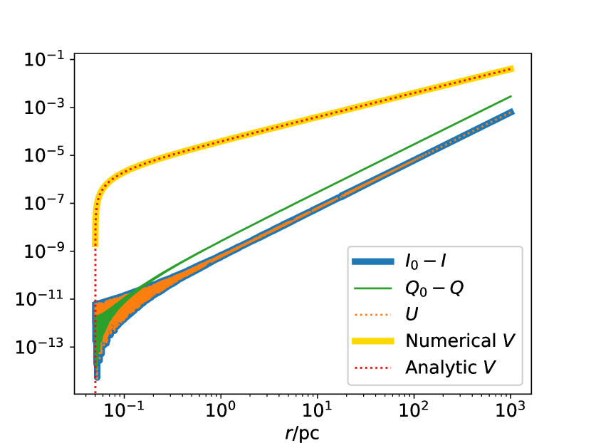
Figure 1: The evolution of Stokes parameters through the jet with the distance $r$. The $Q_{0}$ and $I_{0}$ represent the initial value at $r_{\text{E}}$. Relevant parameters are set to be their typical value while $\Pi_{L}=0.3$ and $m_{a}=10^{-15}~{}\mathrm{eV}$. The value of $\mathcal{V}$ is chosen to be equal to $-\Pi_{L}$ in order to maximize the ALP effect.

From Fig. 1, we can see that the analytic result of $V$ derived from Eq. (45) is consistent with the numerical result. This justifies our analytic formulas. Another interesting feature is that the ALPs can induce a much larger CP compared with LP. Here we give a general qualitative analysis. As long as $P_{\gamma\to a}$ is small, the LP generated by dichroism can be approximated to be the conversion probability, i.e., Eq. (19) Jain et al. (2002); Hutsemekers et al. (2010)

$$\Delta\Pi_{\mathrm{L}}\simeq P_{\gamma\to a}\approx\sin^{2}(2\theta)\sin^{2}(\xi/2),$$ (49)

where $\xi=L/l_{\mathrm{osc}}$ is the ratio of the coherent length of magnetic field to oscillation length. The photons acquire a polarization-dependent phase shift (retardance)

$$\phi_{a}\simeq\sin^{2}(2\theta)(\xi-\sin\xi)$$ (50)

in the mixing with ALPs, which results in CP. If $\phi_{a}\ll 1$, then the CP induced by phase shift can be expressed as

$$V=Q_{0}\sin\phi_{a}\simeq Q_{0}\sin^{2}(2\theta)(\xi-\sin\xi)$$ (51)

with adopting the convention of $U_{0}=0$ and $Q_{0}>0$. For the BL Lacs considered here, the corresponding oscillation length is

$$l_{\mathrm{osc}}\approx|\Delta_{\mathrm{pl}}|^{-1}\approx 9\times 10^{-4}\mathrm{pc}\left(\frac{E}{\mathrm{1eV}}\right)\left(\frac{n_{e}}{1\mathrm{cm}^{-3}}\right)^{-1}.$$ (52)

It is obvious that the oscillation length is far less than the scale of the jet $l_{\mathrm{osc}}\ll r_{\mathrm{max}}$, supposing the magnetic field is coherent over the entire jet region. Thus, the CP produced by the mixing is much larger than that of LP. Besides, Eq. (49) can also explain the oscillatory behavior of $I$ and $U$ in Fig. 1.

In Fig. 2 we demonstrate a similar case, in which all parameters remain unchanged except that $m_{a}=10^{-11}~{}\mathrm{eV}$. We find that when $n_{\mathrm{e}}$ approaches $1~{}\mathrm{cm}^{-3}$, crossing the turning point where the resonant conversion occurs, the behavior of mixing is totally different. This is because the weak-mixing condition Eq. (44) is no longer satisfied, and hence Eq. (45) is not applicable.

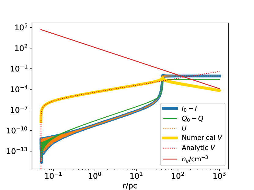
Figure 2: Similar to Fig. 1 except that $m_{a}=10^{-11}~{}\mathrm{eV}$. The red solid line represents the value of electron number density in unit of $\mathrm{cm}^{-3}$.

A few attempts have been made to measure optical CP in blazars Hutsemekers et al. (2010); Valtaoja et al. (1993); Wagner and Mannheim (2001), however no definite optical CP in blazars has been detected. Hutsemékers et al. Hutsemekers et al. (2010) reported null detection of CP with typical uncertainties $<0.1\%$ in 21 quasars, except for two highly polarized blazars. There has not been a confident detection of optical CP in BL Lacs so far. However, some observations still reported tentative results of optical CP in some sources, such as the blazar 3C 66A Takalo and Sillanpaa (1993); Tommasi, L. et al. (2001). We will discuss the ALP interpretation of these observations in the next section.

Considering a detection sensitivity at the level of $\sim 0.1\%$, Eq. (45) can directly give a constraint of $g_{a\gamma}\cdot B_{\mathrm{T0}}\lesssim 7.9\times 10^{-12}~{}\mathrm{G\cdot GeV}^{-1}$, i.e., $g_{a\gamma}\lesssim 7.9\times 10^{-12}~{}\mathrm{GeV}^{-1}$ for $B_{\mathrm{T0}}=1~{}\mathrm{G}$. Compared to leptonic models, hadronic models posses a higher magnetic field strength and less electron density, and thus can give more stringent constraints on the ALP-photon coupling. For example, $B_{\mathrm{T0}}\sim 10~{}\mathrm{G}$ would require $g_{a\gamma}\lesssim 7.9\times 10^{-13}~{}\mathrm{GeV}^{-1}$ assuming the same electron density. In Fig. 3, we demonstrate the constraints on $g_{a}\gamma$ for different choices of $B_{\mathrm{T0}}$ and $n_{\text{e0}}$. For comparison, some previous bounds in the literature are also included Anastassopoulos et al. (2017); Payez et al. (2015); Berg et al. (2017); Marsh et al. (2017).

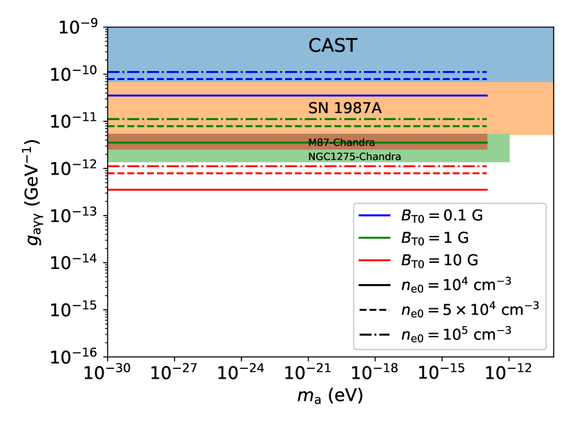
Figure 3: Bounds on the ALP-photon coupling in comparison to previously obtained bounds Anastassopoulos et al. (2017); Payez et al. (2015); Berg et al. (2017); Marsh et al. (2017).

It is worth noting that the above constraints are derived for the optimal case $\mathcal{V}=\pm\Pi_{\mathrm{L}}$, while the value of $\mathcal{V}$ is supposed to be smaller in the more realistic case. More detailed discussions on this issue are given in Sec. V.2. The results obtained here are only rough estimation, which are limited by the knowledge of the jet properties as well as the measurement precision of optical CP. There is no doubt that further research of BL Lacs and improvement of future CP measurements in the optical band will significantly improve our results.

IV ALP interpretation of the tentative CP observation

Although no definite optical CP in blazars has been detected, some observations reported tentative optical CP results in a few particular objects. For example, in 2001, Tommasi et al. Tommasi, L. et al. (2001) reported a marginal detection of optical CP at $2\sigma$ level in V and R bands for 3C 66A by using the Nordic Optical Telescope, which gives an upper limit of $\Pi_{\mathrm{C}}<0.4\%$ at $3\sigma$ confidence level. Besides, a $3-6\sigma$ detection of CP with larger values for 3C 66A was also claimed by Takalo and Sillanpaa Takalo and Sillanpaa (1993), using the same telescope in 1993. Moreover, Hutsemékers et al. Hutsemekers et al. (2010) reported small but significant optical CP in two blazars with uncertainties $<0.1\%$. These tentative observations could be interpreted by the ALPs in the context. Noting that the two blazars in Hutsemekers et al. (2010) are not BL Lacs, the model adopted in Sec. III.1 may not be applicable. Therefore, we put these two objects aside and focus on the 3C 66A at first. Besides, considering that the state of LP was uncertain and the amount of data is inadequate in the research of Tommasi et al. Tommasi, L. et al. (2001), we only analyze the data given by Takalo and Sillanpaa Takalo and Sillanpaa (1993).

The handness of CP changed during the measurement in Takalo and Sillanpaa (1993). This implies that $\phi-\psi\approx k\pi/2$ with $k\in\mathbb{Z}$ in the ALP scenario. Hence, we can make the approximation $\mathcal{V}\approx 2\Pi_{\mathrm{L}}(\phi-\psi)$ in Eq. (36) and obtain

$$\frac{\Pi_{\mathrm{C}}}{\Pi_{\mathrm{L}}E^{\prime}}\propto g_{a\gamma}^{2}\epsilon_{Be}f_{\gamma}\delta^{-1}r_{\mathrm{max}}(\psi-\phi).$$ (53)

The observations were made in the UBVRI photometric systems. Taking into account the effective energy of the color bands, we implement a linear polynomial fit between $\Pi_{\mathrm{C}}/(\Pi_{\mathrm{L}}E^{\prime})$ and the polarization angle $\psi$. The results are shown in Fig. 4 and Table. 1. Here, we have supposed that the orientation of the magnetic field is fixed. Owing to the small value of the CP, the quality of our analysis is sensitive to the accuracy of the polarization angle. It can be seen from Fig. 4 that the data points of RI bands are distributed differently from those of UBV bands. This may be attributed to the systematic differences caused by the two kinds of photomultiplier tubes in the UBV and RI channels. Physical processes that result in the energy dependent rotation of the polarization angle can also affect the distribution. We consider two cases here: one includes the RI bands, while the other not. The potential rotation of the photon polarization angle generated by other effects in the propagation through the astronomical space is neglected in the fitting.

Figure 4: Linear polynomial fit between the polarization angle $\psi$ and $\frac{\Pi_{\mathrm{C}}}{\Pi_{\mathrm{L}}}\frac{2~{}\mathrm{eV}}{E^{\prime}}$, using polarization observation data of 3C 66A in Takalo and Sillanpaa (1993). The letters UBVRI represent different band filters.

Bands	$a_{0}$	$\sigma_{a_{0}}$	$a_{1}$	$\sigma_{a_{1}}$
UBVRI	$-0.39$	0.45	0.62	0.66
UBV	$-4.0$	1.1	5.7	1.6

Table 1: Coefficients of linear polynomial fit to observation in 3C 66A in form of $\frac{\Pi_{\mathrm{C}}}{\Pi_{\mathrm{L}}}\frac{2~{}\mathrm{eV}}{E^{\prime}}=a_{0}+a_{1}\psi$. Parameters are in unit of $10^{-1}$.

As shown in Table. 1, no clear physical conclusion can be drawn from the fit in the UBVRI case, due to the large standard error compared to the corresponding fitting parameters. In the UBV case, the direction of the transverse magnetic field of the jet $\phi$ is estimated to be $0.70~{}\mathrm{rad}$ (40.3°) or $3.84~{}\mathrm{rad}$ (220.4°). From the slope of the line, we obtain

$$g_{a\gamma}\approx 7\times 10^{-11}~{}\mathrm{GeV}^{-1}\left[\epsilon_{Be}f_{\gamma}\left(\frac{15.64}{\delta}\right)\left(\frac{r_{\mathrm{max}}}{1~{}\mathrm{kpc}}\right)\right]^{-1/2}.$$ (54)

The jet model fitting to the observed SED and optical variability patterns of 3C 66A usually gives $\delta\sim 30$ and $f_{\gamma}\approx 1$ Abdo et al. (2011); Boettcher et al. (2013); Reimer et al. (2009). In the leptonic models, a pure SSC model would require a tiny equipartition ratio $\epsilon_{Be}$ $\sim 10^{-3}$, while in the EC+SSC models $\epsilon_{Be}$ would be rather larger $\sim 0.1$ Abdo et al. (2011); Boettcher et al. (2013). Consequently, the EC+SSC models give $g_{a\gamma}\approx 3\times 10^{-10}~{}\mathrm{GeV}^{-1}\sqrt{1~{}\mathrm{kpc}/r_{\mathrm{max}}}$, therefore the ALP interpretation in the leptonic models are excluded by CAST. In the hadronic models with the equipartition ratio $\epsilon_{Be}\sim 25$ Boettcher et al. (2013), we can get $g_{a\gamma}\approx 2\times 10^{-11}~{}\mathrm{GeV}^{-1}\sqrt{1~{}\mathrm{kpc}/r_{\mathrm{max}}}$.

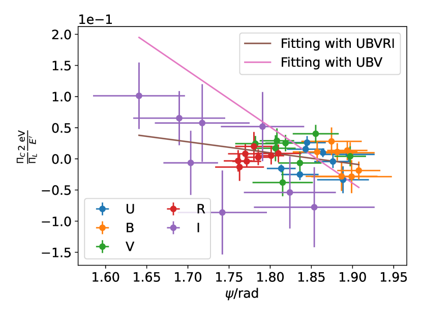
Figure 5: Linear polynomial fit between the polarization angle $\psi$ and $\frac{\Pi_{\mathrm{C}}}{\Pi_{\mathrm{L}}}\frac{2~{}\mathrm{eV}}{E^{\prime}}$, using polarization observation data of OJ 287 in Takalo and Sillanpaa (1993). The letters UBVRI represent different band filters.

Bands	$a_{0}$	$\sigma_{a_{0}}$	$a_{1}$	$\sigma_{a_{1}}$
UBVRI	3.3	1.5	$-1.8$	0.79
UBV	16.8	6.4	$-9.0$	3.5

Table 2: Coefficients of linear polynomial fit to observation in OJ 287 in form of $\frac{\Pi_{\mathrm{C}}}{\Pi_{\mathrm{L}}}\frac{2~{}\mathrm{eV}}{E^{\prime}}=a_{0}+a_{1}\psi$. Parameters are in unit of $10^{-1}$.

Apart from 3C 66A, Takalo and Sillanpaa indicated a rapid variability in the U-band CP during the observation of OJ 287. Although the nightly average CP observation did not find optical CP, we can still repeat the above analysis procedure for this object, and provide the results in Fig. 5 and Table. 2. Similarly, we get a model-dependent estimation for $g_{a\gamma}$, listing in Table. 3.

The observations of these objects indicate a similar estimation for $g_{a\gamma}$, which is about a few orders of $10^{-11}~{}\mathrm{GeV}^{-1}$. However, we emphasize that the validity of such results strongly depends on the accuracy of the optical polarimetry. Simultaneous LP and CP measurements in the optical band with high accuracy are needed to verify this analysis in the future.

Bands	$\phi(rad)$	$g_{a\gamma}(\times 10^{-11}~{}\mathrm{GeV}^{-1})$
		Leptonic	Hadronic
UBVRI	0.26 or 3.40	1.3	0.70
UBV	0.30 or 3.44	2.9	1.6

Table 3: Estimation of $\phi$ and $g_{a\gamma}$ using fitting coefficients in OJ 287. The factor $\sqrt{1~{}\mathrm{kpc}/r_{\mathrm{max}}}$ in $g_{a\gamma}$ is omitted. $\delta=15$. $f_{\gamma}\approx 1.2,~{}\epsilon_{Be}=8.2$ for leptonic model and $f_{\gamma}\approx 0.5,~{}\epsilon_{Be}=66$ for hadronic model Boettcher et al. (2013).

V Discussions

As mentioned in Sec. III.2, Eq. (45) is idealized in some sense. In this section, we discuss some relevant physical factors that may affect the above results.

V.1 Intrinsic CP

On the astrophysical origin of optical CP in blazars, the inverse Compton scattering of radio photons with high CP and the intrinsic CP are two likely options Rieger and Mannheim (2005). However, the former mechanism requires the significant radio CP and SSC contribution to optical continuum, which are not observed. Therefore, we discuss the consequence that the intrinsic CP is present in this subsection.

The synchrotron radiation of particles generates a small degree of intrinsic CP with $\Pi_{\mathrm{C}}\propto\nu^{-1/2}$ Legg and Westfold (1968); Melrose (1971). In a pure electron-positron plasma, the CP component cancels, leaving only the LP component. Assuming an electron-positron-proton plasma with $f$ denoting the fraction of the positron in the jet, the degree of the intrinsic CP can be characterized as Rieger and Mannheim (2005)

$$\Pi_{\mathrm{C}}\approx 2.8\times 10^{-2}\left(\frac{B}{1~{}\mathrm{G}}\right)^{1/2}\left(\frac{E^{\prime}}{1~{}\mathrm{eV}}\right)^{-1/2}\left(\frac{\Pi_{\mathrm{L}}}{0.71}\right)\left(\frac{\Gamma}{15}\right)^{3/2}(1-2f),$$ (55)

where the Lorentz factor $\Gamma$ can be approximated by $\delta$ in the highly collimated regime. Detecting upper limits of the intrinsic CP of two blazars, Liodakis et al. Liodakis et al. (2021) claimed the exclusion of high-energy emission models with the high magnetic field strength and low positron fraction, like the hadronic models.

However, the ALP induced CP may offset the intrinsic CP, since the handness of the ALP induced CP can be either positive or negative, which is determined by the angle between the magnetic field and photon polarization. From the view of the observer, the handness of CP is positive, if the direction of the transverse magnetic field lies in $I,III$ quadrants of the Cartesian coordinate system with the direction of polarization as the x-axis. Thus, we study the case that ALPs induce a negative CP in the hadronic model. We calculate the sum of two kinds of CP origins with $B$ in the range of $[0,10]~{}\mathrm{G}$ and $[0,0.5)$ for $f$. In order to get comparable values, we choose $g_{a\gamma}=5\times 10^{-12}~{}\mathrm{GeV}^{-1}$ and $\phi=\pi/4$ while keeping other parameters unchanged. As shown in Fig. 6, there exists a large parameter region where optical CP does not exceed the precision of measurements even for the large magnetic field strength and low positron fraction. A smaller coupling $g_{a\gamma}$ indicates the possibility of a larger magnetic field. In order to discriminate these two scenarios, it is crucial to measure the radio and optical CP simultaneously. This is because that the radio CP is expected to be associated with the intrinsic CP, while ALPs considered here have little effect on the radio photons.

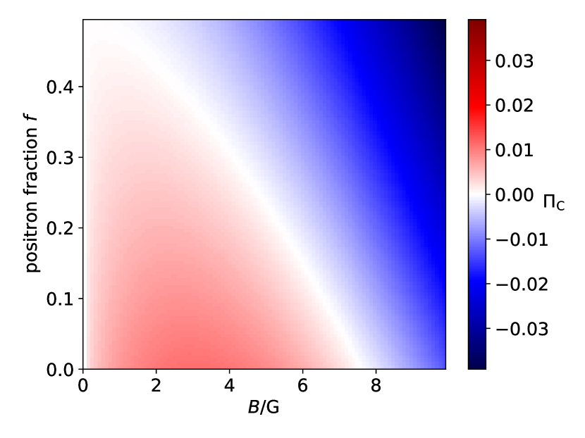
Figure 6: The degree of optical CP of blazars with different magnetic field strength $B$ and plasma composition characterized by $f$.

V.2 Structure of the jet

In the above analysis, the angle of the transverse magnetic field is idealized, fixing to $3\pi/4$ or $\pi/4$. However, for a more realistic case, the direction of magnetic field could change in the jet and result in a shorter coherent length, which in turn leads to a smaller CP. In order to estimate this effect, we assume that the direction of the magnetic field is partially random in each calculation domain, i.e.,

$$\phi=\phi_{0}+\alpha\Delta\phi,$$ (56)

where $\phi_{0}=3\pi/4$ and $\Delta\phi$ is a uniform random variable in the range of $[-\pi,\pi]$. The factor $\alpha$ characterizes the degree of randomness. Similar to what we have done in Sec. III.2, examples of the evolution of the Stokes parameters with $\alpha=0.1,0.2,0.3$ and $\mathcal{R}=0.001,0.01,0.1$ are shown in Fig. 7. The coherent length of the magnetic field (also the number of domains) is determined by the decrease ratio $\mathcal{R}$. As shown in Fig. 7, the values of $\alpha$ and $\mathcal{R}$ can significantly change the pattern of the evolution. As $\alpha$ increases, the evolution shows more randomness and quiver. Moreover, for each set of parameters, we demonstrate the distribution of CP sampled for 1000 sets of magnetic field configurations in Fig. 8. It shows that for a more realistic field configuration, the values of CP are smaller than the optimal case, while its magnitude remains in the same order.

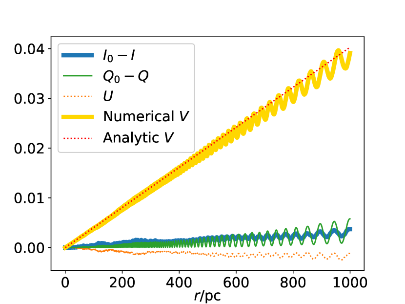
(a)  $\alpha=0.1,~{}\mathcal{R}=0.001$

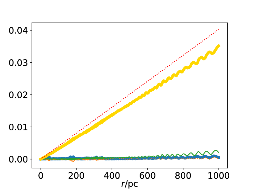
(b)  $\alpha=0.2,~{}\mathcal{R}=0.001$

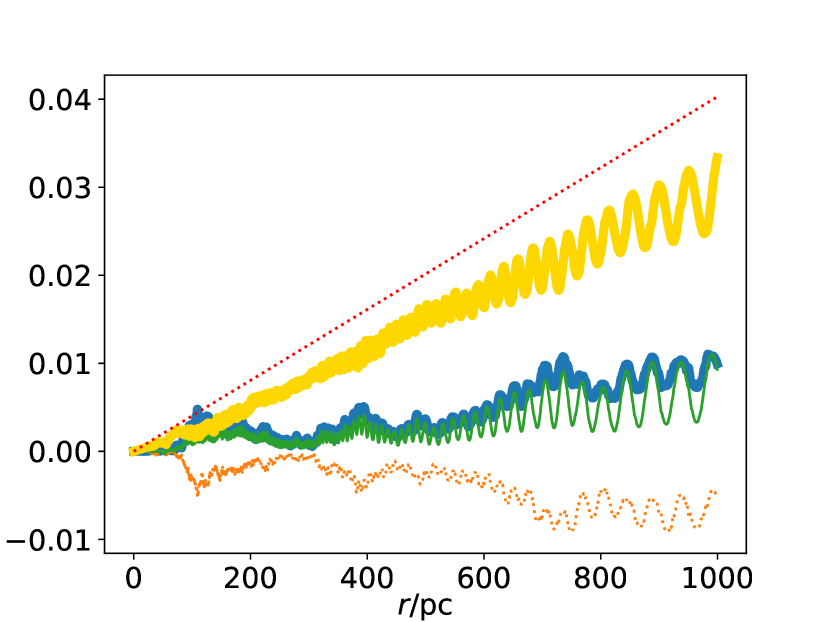
(c)  $\alpha=0.3,~{}\mathcal{R}=0.001$

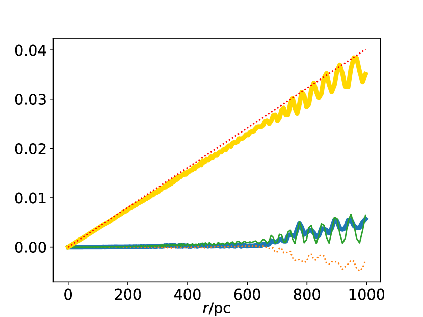
(d)  $\alpha=0.1,~{}\mathcal{R}=0.01$

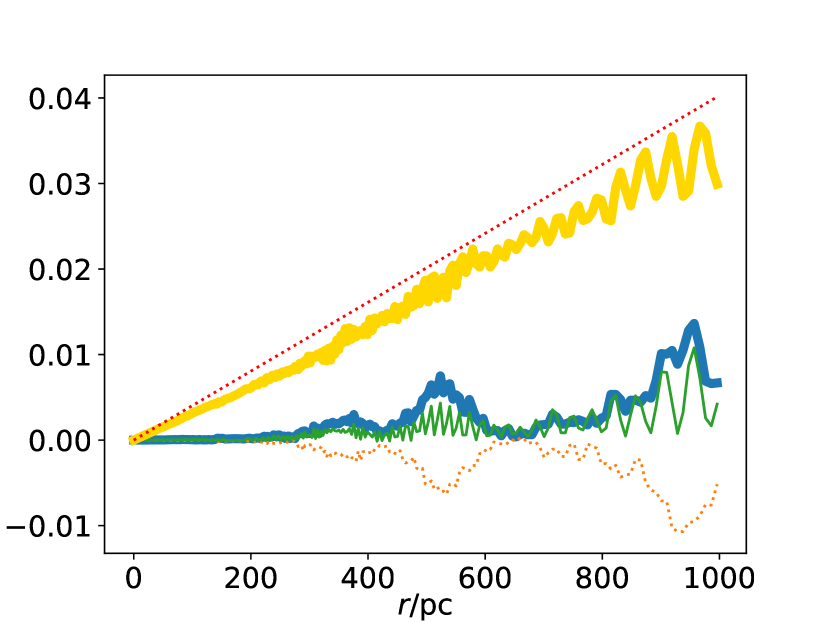
(e)  $\alpha=0.2,~{}\mathcal{R}=0.01$

(f)  $\alpha=0.3,~{}\mathcal{R}=0.01$

(g)  $\alpha=0.1,~{}\mathcal{R}=0.1$

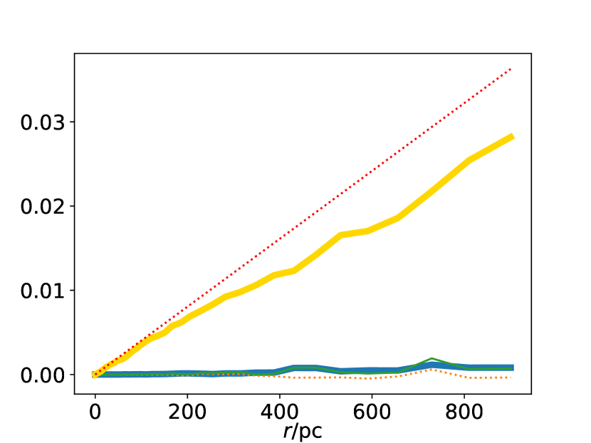
(h)  $\alpha=0.2,~{}\mathcal{R}=0.1$

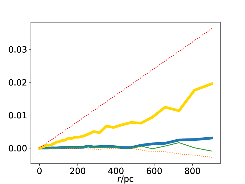
(i)  $\alpha=0.3,~{}\mathcal{R}=0.1$

Figure 7: Examples of evolution of Stokes parameters for magnetic field with varied angle in different cases. The configuration of jet is sliced into domains, determined by the decrease ratio $\mathcal{R}$. The angle in each domain is $\phi=\phi_{0}+\alpha\Delta\phi$ with $\phi_{0}=3\pi/4$ and a uniform random variable $\Delta\phi$ in the $[-\pi,\pi]$ range.

Next, we give a qualitative analysis of the results in Fig. 7 and Fig. 8. Given the approximation that $\alpha\ll 1$ is true, we can rewrite Eq. (39) as

$$\mathcal{V}_{\mathrm{n+1}}\approx\Pi_{\mathrm{L}}\sin 2(\phi_{\mathrm{0}}-\psi_{\mathrm{n}})+2\alpha\Delta\phi_{\mathrm{n}}\Pi_{\mathrm{L}}\cos 2(\phi_{\mathrm{0}}-\psi_{\mathrm{n}}),$$ (57)

where the subscription $n$ indicates the $n$th domain. Then the change of $V$ is determined by two parts: the incremental part (the first term) and the random part (the second term). Also, Eq. (36) is applicable for the incremental part in each domain, which explains the magnitude of the expectation value of the CP. When $\phi_{\mathrm{0}}=3\pi/4$, the second term can be written as $-2\alpha\Delta\phi_{\mathrm{n}}U_{\mathrm{n}}$. Hence, as shown in Fig. 7, the quiver of $V$ in each domain is related to the magnitude of $U$ of the former domain. As for the contribution of the random part, it can be treated as a random walk, thus its variance is estimated to be $2\alpha\langle\Delta\phi_{\mathrm{n}}U_{\mathrm{n}}\rangle\sqrt{N}$, where $N$ is the number of domains and the angle bracket means the expectation value. Therefore, with the increase of $\alpha$, the randomness of the evolution of CP degree becomes stronger.

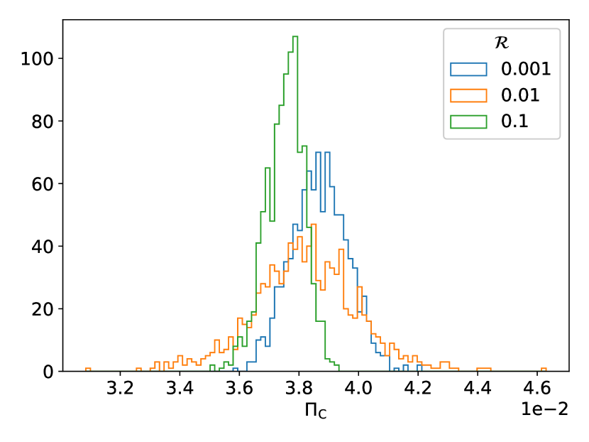
(a)  $\alpha=0.1$

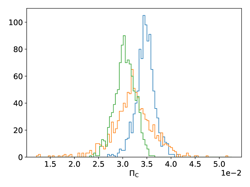
(b)  $\alpha=0.2$

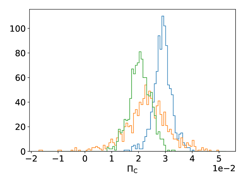
(c)  $\alpha=0.3$

Figure 8: Similar to Fig. 7. Distribution of optical CP induced by ALPs for magnetic field with varied angle in different cases.

In addition, considering the limit of the spatial resolution of the detector, the photons received by the detector are not from a certain point on the source but from the whole emitting region. In this case, the direction of the transverse magnetic field may be spatial dependent. In order to have a rough idea of this effect, we can replace the $\mathcal{V}$ in Eq. (36) with $\int_{\phi_{1}}^{\phi_{2}}\mathcal{V}(\phi)d\phi/(\phi_{2}-\phi_{1})$, assuming the direction angle of the transverse magnetic field in the region evenly varies from $\phi_{1}$ to $\phi_{2}$ and the initial photons from different positions have the same polarization state. In practice, the density matrices of photons are calculated in multi paths, where Eq. (56) is still adopted but the values of $\phi_{0}$ evenly vary in different paths. Then summing all density matrices, we obtain the assembly CP in a specific range of $\phi_{0}$ in the numerical calculation.

In Fig. 9, we show the distribution of assembly CP for the partially random magnetic fields in three intervals of $\phi_{0}$. Note that a toroidal transverse magnetic field for $\phi_{0}$ is assumed here. This indicates that the transverse magnetic field roughly follows a uniform distribution. The decrease ratio is chosen to be $\mathcal{R}=0.1$ for simplicity. These subfigures can be recognized as the distribution of the observed CP in blazars with different measurement precision. We find that the assembly CP significantly cancels in the first two cases, leading to a zero expectation, while the third case shows a moderate CP. This shows that high-precision measurements are needed to observe optical CP in a large sample. Nevertheless, even in the low-precision cases, it is possible that there are some blazars that can produce observable CP.

Note that the above results base on the assumption that the transverse magnetic field roughly follows a uniform distribution. However, the most probable distribution of the direction of the magnetic field is very likely to significantly deviate from the uniform distribution in reality, considering the relativistic beaming effect, the jet angle with respect to the line-of-sight, and the complexity of the structure of the jet magnetic field. Consequently, the expectation of the realistic observed CP distribution is unlikely to be zero and would still indicate possible significant signatures. However, a complete and accurate survey of the distribution depends on an in-depth study of the magnetic field configuration in blazars. The detailed study on this issue is beyond the scope of this paper, so it is left to follow-up research. More studies on the blazar jets and high-precision measurements are needed to get more reliable conclusions.

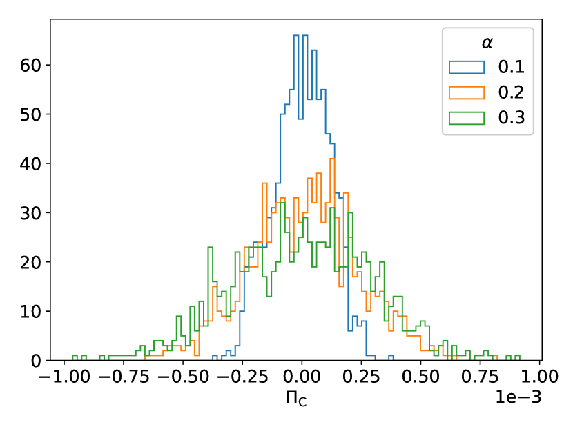
(a)  $\phi_{\mathrm{0}}:0\sim 2\pi$

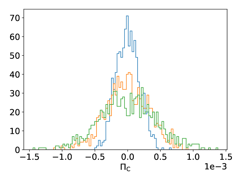
(b)  $\phi_{\mathrm{0}}:0\sim\pi$

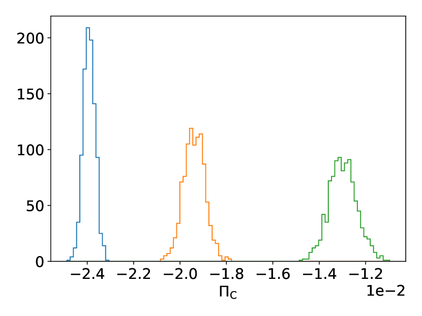
(c)  $\phi_{\mathrm{0}}:0\sim\pi/2$

Figure 9: Distribution of assembly optical CP for partially random magnetic field with $\phi_{0}$ in different intervals. The decrease ratio is chosen to be $\mathcal{R}=0.1$ for simplicity.

V.3 CP in other astrophysical magnetic fields

Magnetic fields are ubiquitous in the propagation of photons from blazars to Earth. The ALP-photon mixing in other astrophysical magnetic fields may contribute to optical CP and alter the results obtained above. For completeness, we give a rough estimation of these effects. According to Eq. (51), the contribution of mixing is $\sim\Pi_{\mathrm{L}}g_{a\gamma}^{2}B^{2}l_{\mathrm{osc}}L$ as long as the weak-mixing condition is fulfilled. Here we define a new quantity, i.e.,

$$f_{\mathrm{CP}}=\left(\frac{B}{1~{}\mathrm{G}}\right)^{2}\left(\frac{n_{\mathrm{e}}}{5\times 10^{4}~{}\mathrm{cm}^{-3}}\right)^{-1}\left(\frac{L}{1~{}\mathrm{kpc}}\right),$$ (58)

which straightforwardly characterizes the contribution to CP due to the ALP-photon mixing in different magnetic fields. For example, for BL Lacs considered in this paper, we can get $f_{\mathrm{CP}}\simeq 1$. In Table. 4, we show the value of $f_{\mathrm{CP}}$ for different magnetic field scenarios, including the magnetic field inside a galaxy cluster (intra-cluster magnetic field, ICMF), the intergalactic magnetic field (IGMF), and the galactic magnetic field in the Milky Way (GMF). For each scenario, the typical values of $B$, $n_{\mathrm{e}}$, and coherent length scale $L$ are also given. Considering that the turbulent magnetic field configuration is usually used in these fields, the situation is closer to the random walk case that we discuss in the former part, and the output relies on the specific realization of the magnetic field. From Table. 4, we can see that the influence of other astrophysical magnetic fields can be neglected.

Scenarios	$B(\mathrm{G})$	$n_{\mathrm{e}}(\mathrm{cm}^{-3})$	$L(\mathrm{kpc})$	$f_{\mathrm{CP}}$
ICMF Govoni and Feretti (2004); Feretti et al. (2012)	$10^{-6}$	$10^{-3}$	$10$	$5\times 10^{-4}$
IGMF Blasi et al. (1999); De Angelis et al. (2008); Abreu et al. (2010); Hinshaw et al. (2013)	$10^{-9}$	$10^{-7}$	$5\times 10^{4}$	$2.5\times 10^{-2}$
GMF Jansson and Farrar (2012a, b)	$10^{-6}$	$10^{-1}$	$10^{-2}$	$5\times 10^{-9}$

Table 4: The value of $f_{\mathrm{CP}}$ for different magnetic field scenarios.

Apart from the astrophysical magnetic fields mentioned above, the field in the supercluster has been discussed in Payez et al. (2011, 2012). The ALP-photon mixing in the supercluster was originally proposed to explain the alignments of the optical polarization of light from quasars in extremely large regions of the sky, but disfavored by subsequent study. The effect of the supercluster needs to be taken into account when it intervenes in the line-of-sight of blazars. The authors of Payez et al. (2012) claimed to constrain $g_{a\gamma}\lesssim 10^{-13}~{}\mathrm{GeV}^{-1}$ for $m_{\mathrm{a}}\lesssim 10^{-14}~{}\mathrm{eV}$, which would be the most stringent limit to date. They assumed the electron density of $\mathcal{O}(10^{-6})~{}\mathrm{cm}^{-3}$ and the magnetic field of $\mathcal{O}(\mu\mathrm{G})$ with the coherent length $\sim 100~{}\mathrm{kpc}$ in the supercluster. This configuration of the supercluster field would give $f_{\mathrm{CP}}\sim 5$. However, the studies of supercluster magnetic fields Dolag et al. (2005); Bregman et al. (2004); Suhhonenko et al. (2011); Einasto et al. (2014); Tully et al. (2014); Einasto et al. (2020) find that their structures are filamentous. There is no firm conclusion about the magnetic field strength in galaxy filaments within the supercluster, neither from observations nor from theory Dolag et al. (2005); Vazza et al. (2015, 2021); Oei et al. (2022). It seems that the field strength considered in Payez et al. (2012) is overestimated, and the strict constraint would be relaxed to some extent. Despite this, it will help to restrict our results even if optical CP is produced in the supercluster.

VI Conclusions

In this work, we investigate a potential optical CP in blazars induced by the ALP-photon mixing. Although this mixing is weak and has little effect on the flux and LP of photons, we have shown that it could induce a considerable optical CP when the oscillation length is much less than the coherent length of the magnetic field in the blazar jet. The formulas of the ALP induced CP in a simple conical jet are derived, which lead to a constraint on $g_{a\gamma}$, i.e., $g_{a\gamma}\cdot B_{\mathrm{T0}}\lesssim 7.9\times 10^{-12}~{}\mathrm{G\cdot GeV}^{-1}$ for $m_{a}\lesssim 10^{-13}~{}\mathrm{eV}$, corresponding to the upper limit on the observed CP at the level of $\sim 0.1\%$. Hence, the coupling between the ALP and photon would be significantly constrained in the hadronic radiation model with a large magnetic field strength in the jet. Further research on BL Lacs and CP measurement in the optical band would significantly improve these results.

In particular, the tentative CP observations of two blazar 3C 66A and OJ 287 induced by ALP are analyzed using the data in the paper of Takalo and Sillanpaa. We find that these observations indicate a similar estimation of $g_{a\gamma}\sim 10^{-11}~{}\mathrm{GeV}^{-1}$. Large amount of simultaneous LP and CP measurements with high accuracy in the future are needed to verify the irregular results.

Though hadronic models set stringent constraint on $g_{a\gamma}$, the results could be significantly changed considering the intrinsic CP. Measuring the radio and optical CP simultaneously would be helpful to clarify the situation. Besides, note that many results of the ALP induced CP in this work are derived with an idealized jet configuration. As stated in the last part of Sec.V, we have shown that the obtained results are partially valid in more realistic cases.

Note added.—During the completion of the paper, we became aware of a work Shakeri and Hajkarim (2022) which also considers a similar topic. The axion-induced CP of light around black holes with some different physical settings is studied in that paper.

References

- Witten (1984) E. Witten, Phys. Lett. B 149, 351 (1984).
- Svrcek and Witten (2006) P. Svrcek and E. Witten, JHEP 06, 051 (2006), arXiv:hep-th/0605206 .
- Conlon (2006a) J. P. Conlon, JHEP 05, 078 (2006a), arXiv:hep-th/0602233 .
- Conlon (2006b) J. P. Conlon, Phys. Rev. Lett. 97, 261802 (2006b), arXiv:hep-ph/0607138 .
- Arvanitaki et al. (2010) A. Arvanitaki, S. Dimopoulos, S. Dubovsky, N. Kaloper, and J. March-Russell, Phys. Rev. D 81, 123530 (2010), arXiv:0905.4720 [hep-th] .
- Acharya et al. (2010) B. S. Acharya, K. Bobkov, and P. Kumar, JHEP 11, 105 (2010), arXiv:1004.5138 [hep-th] .
- Cicoli et al. (2012) M. Cicoli, M. Goodsell, and A. Ringwald, JHEP 10, 146 (2012), arXiv:1206.0819 [hep-th] .
- Peccei and Quinn (1977a) R. D. Peccei and H. R. Quinn, Phys. Rev. Lett. 38, 1440 (1977a).
- Peccei and Quinn (1977b) R. D. Peccei and H. R. Quinn, Phys. Rev. D 16, 1791 (1977b).
- Weinberg (1978) S. Weinberg, Phys. Rev. Lett. 40, 223 (1978).
- Wilczek (1978) F. Wilczek, Phys. Rev. Lett. 40, 279 (1978).
- Cheng (1988) H.-Y. Cheng, Phys. Rept. 158, 1 (1988).
- Kolb and Turner (1990) E. W. Kolb and M. S. Turner, The Early Universe, Vol. 69 (CRC Press, 1990).
- Turner (1990) M. S. Turner, Phys. Rept. 197, 67 (1990).
- Sikivie (2008) P. Sikivie, Lect. Notes Phys. 741, 19 (2008), arXiv:astro-ph/0610440 .
- Carroll (1998) S. M. Carroll, Phys. Rev. Lett. 81, 3067 (1998), arXiv:astro-ph/9806099 .
- Marsh (2016) D. J. E. Marsh, Phys. Rept. 643, 1 (2016), arXiv:1510.07633 [astro-ph.CO] .
- Preskill et al. (1983) J. Preskill, M. B. Wise, and F. Wilczek, Phys. Lett. B 120, 127 (1983).
- Abbott and Sikivie (1983) L. F. Abbott and P. Sikivie, Phys. Lett. B 120, 133 (1983).
- Dine and Fischler (1983) M. Dine and W. Fischler, Phys. Lett. B 120, 137 (1983).
- Graham et al. (2015) P. W. Graham, I. G. Irastorza, S. K. Lamoreaux, A. Lindner, and K. A. van Bibber, Ann. Rev. Nucl. Part. Sci. 65, 485 (2015), arXiv:1602.00039 [hep-ex] .
- Fedderke et al. (2019) M. A. Fedderke, P. W. Graham, and S. Rajendran, Phys. Rev. D 100, 015040 (2019), arXiv:1903.02666 [astro-ph.CO] .
- Schwarz et al. (2021) D. J. Schwarz, J. Goswami, and A. Basu, Phys. Rev. D 103, L081306 (2021), arXiv:2003.10205 [hep-ph] .
- Ivanov et al. (2019) M. M. Ivanov, Y. Y. Kovalev, M. L. Lister, A. G. Panin, A. B. Pushkarev, T. Savolainen, and S. V. Troitsky, JCAP 02, 059 (2019), arXiv:1811.10997 [astro-ph.CO] .
- DeRocco and Hook (2018) W. DeRocco and A. Hook, Phys. Rev. D 98, 035021 (2018), arXiv:1802.07273 [hep-ph] .
- Obata et al. (2018) I. Obata, T. Fujita, and Y. Michimura, Phys. Rev. Lett. 121, 161301 (2018), arXiv:1805.11753 [astro-ph.CO] .
- Caputo et al. (2019) A. Caputo, L. Sberna, M. Frias, D. Blas, P. Pani, L. Shao, and W. Yan, Phys. Rev. D 100, 063515 (2019), arXiv:1902.02695 [astro-ph.CO] .
- Chen et al. (2020) Y. Chen, J. Shu, X. Xue, Q. Yuan, and Y. Zhao, Phys. Rev. Lett. 124, 061102 (2020), arXiv:1905.02213 [hep-ph] .
- Yuan et al. (2021) G.-W. Yuan, Z.-Q. Xia, C. Tang, Y. Zhao, Y.-F. Cai, Y. Chen, J. Shu, and Q. Yuan, JCAP 03, 018 (2021), arXiv:2008.13662 [astro-ph.HE] .
- Sikivie (1983) P. Sikivie, Phys. Rev. Lett. 51, 1415 (1983), [Erratum: Phys.Rev.Lett. 52, 695 (1984)].
- Raffelt and Stodolsky (1988) G. Raffelt and L. Stodolsky, Phys. Rev. D 37, 1237 (1988).
- Maiani et al. (1986) L. Maiani, R. Petronzio, and E. Zavattini, Phys. Lett. B 175, 359 (1986).
- Csaki et al. (2003) C. Csaki, N. Kaloper, M. Peloso, and J. Terning, JCAP 05, 005 (2003), arXiv:hep-ph/0302030 .
- De Angelis et al. (2007) A. De Angelis, M. Roncadelli, and O. Mansutti, Phys. Rev. D 76, 121301 (2007), arXiv:0707.4312 [astro-ph] .
- Hooper and Serpico (2007) D. Hooper and P. D. Serpico, Phys. Rev. Lett. 99, 231102 (2007), arXiv:0706.3203 [hep-ph] .
- Simet et al. (2008) M. Simet, D. Hooper, and P. D. Serpico, Phys. Rev. D 77, 063001 (2008), arXiv:0712.2825 [astro-ph] .
- Sanchez-Conde et al. (2009) M. A. Sanchez-Conde, D. Paneque, E. Bloom, F. Prada, and A. Dominguez, Phys. Rev. D 79, 123511 (2009), arXiv:0905.3270 [astro-ph.CO] .
- Mirizzi and Montanino (2009) A. Mirizzi and D. Montanino, JCAP 12, 004 (2009), arXiv:0911.0015 [astro-ph.HE] .
- Bassan et al. (2010) N. Bassan, A. Mirizzi, and M. Roncadelli, JCAP 05, 010 (2010), arXiv:1001.5267 [astro-ph.HE] .
- De Angelis et al. (2011) A. De Angelis, G. Galanti, and M. Roncadelli, Phys. Rev. D 84, 105030 (2011), [Erratum: Phys.Rev.D 87, 109903 (2013)], arXiv:1106.1132 [astro-ph.HE] .
- Galanti et al. (2019) G. Galanti, F. Tavecchio, M. Roncadelli, and C. Evoli, Mon. Not. Roy. Astron. Soc. 487, 123 (2019), arXiv:1811.03548 [astro-ph.HE] .
- Dessert et al. (2020) C. Dessert, J. W. Foster, and B. R. Safdi, Phys. Rev. Lett. 125, 261102 (2020), arXiv:2008.03305 [hep-ph] .
- Pshirkov and Popov (2009) M. S. Pshirkov and S. B. Popov, J. Exp. Theor. Phys. 108, 384 (2009), arXiv:0711.1264 [astro-ph] .
- Hook et al. (2018) A. Hook, Y. Kahn, B. R. Safdi, and Z. Sun, Phys. Rev. Lett. 121, 241102 (2018), arXiv:1804.03145 [hep-ph] .
- Huang et al. (2018) F. P. Huang, K. Kadota, T. Sekiguchi, and H. Tashiro, Phys. Rev. D 97, 123001 (2018), arXiv:1803.08230 [hep-ph] .
- Dessert et al. (2019) C. Dessert, A. J. Long, and B. R. Safdi, Phys. Rev. Lett. 123, 061104 (2019), arXiv:1903.05088 [hep-ph] .
- Darling (2020) J. Darling, Phys. Rev. Lett. 125, 121103 (2020), arXiv:2008.01877 [astro-ph.CO] .
- Edwards et al. (2021) T. D. P. Edwards, B. J. Kavanagh, L. Visinelli, and C. Weniger, Phys. Rev. Lett. 127, 131103 (2021), arXiv:2011.05378 [hep-ph] .
- Wang et al. (2021a) J.-W. Wang, X.-J. Bi, R.-M. Yao, and P.-F. Yin, Phys. Rev. D 103, 115021 (2021a), arXiv:2101.02585 [hep-ph] .
- Wang et al. (2021b) J.-W. Wang, X.-J. Bi, and P.-F. Yin, Phys. Rev. D 104, 103015 (2021b), arXiv:2109.00877 [astro-ph.HE] .
- Prabhu (2021) A. Prabhu, Phys. Rev. D 104, 055038 (2021), arXiv:2104.14569 [hep-ph] .
- Dessert et al. (2022) C. Dessert, D. Dunsky, and B. R. Safdi, Phys. Rev. D 105, 103034 (2022), arXiv:2203.04319 [hep-ph] .
- Jain et al. (2002) P. Jain, S. Panda, and S. Sarala, Phys. Rev. D 66, 085007 (2002), arXiv:hep-ph/0206046 .
- Agarwal et al. (2008) N. Agarwal, P. Jain, D. W. McKay, and J. P. Ralston, Phys. Rev. D 78, 085028 (2008), arXiv:0807.4587 [hep-ph] .
- Payez et al. (2011) A. Payez, J. R. Cudell, and D. Hutsemekers, Phys. Rev. D 84, 085029 (2011), arXiv:1107.2013 [astro-ph.CO] .
- Payez et al. (2012) A. Payez, J. R. Cudell, and D. Hutsemekers, JCAP 07, 041 (2012), arXiv:1204.6187 [astro-ph.CO] .
- Tiwari (2017) P. Tiwari, Phys. Rev. D 95, 023005 (2017), arXiv:1610.06583 [astro-ph.CO] .
- Csaki et al. (2002) C. Csaki, N. Kaloper, and J. Terning, Phys. Rev. Lett. 88, 161302 (2002), arXiv:hep-ph/0111311 .
- Grossman et al. (2002) Y. Grossman, S. Roy, and J. Zupan, Phys. Lett. B 543, 23 (2002), arXiv:hep-ph/0204216 .
- Mirizzi et al. (2008) A. Mirizzi, G. G. Raffelt, and P. D. Serpico, Lect. Notes Phys. 741, 115 (2008), arXiv:astro-ph/0607415 .
- Avgoustidis et al. (2010) A. Avgoustidis, C. Burrage, J. Redondo, L. Verde, and R. Jimenez, JCAP 10, 024 (2010), arXiv:1004.2053 [astro-ph.CO] .
- Liao et al. (2015) K. Liao, A. Avgoustidis, and Z. Li, Phys. Rev. D 92, 123539 (2015), arXiv:1512.01861 [astro-ph.CO] .
- Buen-Abad et al. (2022) M. A. Buen-Abad, J. Fan, and C. Sun, JHEP 02, 103 (2022), arXiv:2011.05993 [hep-ph] .
- Meyer et al. (2014) M. Meyer, D. Montanino, and J. Conrad, JCAP 09, 003 (2014), arXiv:1406.5972 [astro-ph.HE] .
- Tavecchio et al. (2015) F. Tavecchio, M. Roncadelli, and G. Galanti, Phys. Lett. B 744, 375 (2015), arXiv:1406.2303 [astro-ph.HE] .
- Day and Krippendorf (2018) F. Day and S. Krippendorf, Galaxies 6, 45 (2018), arXiv:1801.10557 [hep-ph] .
- Galanti (2022a) G. Galanti, Phys. Rev. D 105, 083022 (2022a), arXiv:2202.10315 [hep-ph] .
- Galanti (2022b) G. Galanti, “Photon-ALP oscillations inducing modification on -ray polarization,” (2022b), arXiv:2202.11675 [astro-ph.HE] .
- Galanti et al. (2022) G. Galanti, M. Roncadelli, and F. Tavecchio, “ALP induced polarization effects on photons from galaxy clusters,” (2022), arXiv:2202.12286 [astro-ph.HE] .
- Krawczynski et al. (2016) H. S. Krawczynski et al., Astropart. Phys. 75, 8 (2016), arXiv:1510.08358 [astro-ph.IM] .
- Soffitta (2017) P. Soffitta, in UV, X-Ray, and Gamma-Ray Space Instrumentation for Astronomy XX, Vol. 10397, edited by O. H. Siegmund, International Society for Optics and Photonics (SPIE, 2017) p. 103970I.
- Urry and Padovani (1995) C. M. Urry and P. Padovani, Publ. Astron. Soc. Pac. 107, 803 (1995), arXiv:astro-ph/9506063 .
- Angel and Stockman (1980) J. R. P. Angel and H. S. Stockman, Ann. Rev. Astron. Astrophys. 18, 321 (1980).
- Zhang (2019) H. Zhang, Galaxies 7, 85 (2019).
- Rieger and Mannheim (2005) F. M. Rieger and K. Mannheim, Chinese Journal of Astronomy and Astrophysics 5, 311 (2005).
- Kuster et al. (2008) M. Kuster, G. Raffelt, and B. Beltran, eds., Axions: Theory, cosmology, and experimental searches. Proceedings, 1st Joint ILIAS-CERN-CAST axion training, Geneva, Switzerland, November 30-December 2, 2005, Vol. 741 (2008).
- Galanti and Roncadelli (2018) G. Galanti and M. Roncadelli, Phys. Rev. D 98, 043018 (2018), arXiv:1804.09443 [astro-ph.HE] .
- Davies et al. (2021) J. Davies, M. Meyer, and G. Cotter, Phys. Rev. D 103, 023008 (2021), arXiv:2011.08123 [astro-ph.HE] .
- Dobrynina et al. (2015) A. Dobrynina, A. Kartavtsev, and G. Raffelt, Phys. Rev. D 91, 083003 (2015), [Erratum: Phys.Rev.D 95, 109905 (2017)], arXiv:1412.4777 [astro-ph.HE] .
- Kosowsky (1996) A. Kosowsky, Annals Phys. 246, 49 (1996), arXiv:astro-ph/9501045 .
- Rybicki (2004) G. B. Rybicki, Radiative Processes in Astrophysics (Wiley-VCH, 2004).
- Shaw et al. (2013) M. S. Shaw, R. W. Romani, G. Cotter, S. E. Healey, P. F. Michelson, A. C. S. Readhead, J. L. Richards, W. Max-Moerbeck, O. G. King, and W. J. Potter, Astrophys. J. 764, 135 (2013), arXiv:1301.0323 [astro-ph.HE] .
- Shaw et al. (2012) M. S. Shaw, R. W. Romani, G. Cotter, S. E. Healey, P. F. Michelson, A. C. S. Readhead, J. L. Richards, W. Max-Moerbeck, O. G. King, and W. J. Potter, Astrophys. J. 748, 49 (2012), arXiv:1201.0999 [astro-ph.HE] .
- Pudritz et al. (2012) R. E. Pudritz, M. J. Hardcastle, and D. C. Gabuzda, Space Sci. Rev. 169, 27 (2012), arXiv:1205.2073 [astro-ph.HE] .
- Hutsemekers et al. (2010) D. Hutsemekers, B. Borguet, D. Sluse, R. Cabanac, and H. Lamy, Astron. Astrophys. 520, L7 (2010), arXiv:1009.4049 [astro-ph.CO] .
- Prandini and Ghisellini (2022) E. Prandini and G. Ghisellini, Galaxies 10, 35 (2022), arXiv:2202.07490 [astro-ph.HE] .
- Gabuzda et al. (2004) D. C. Gabuzda, E. Murray, and P. Cronin, Mon. Not. Roy. Astron. Soc. 351, L89 (2004), arXiv:astro-ph/0405394 .
- Gabuzda et al. (2017) D. C. Gabuzda, N. Roche, A. Kirwan, S. Knuettel, M. Nagle, and C. Houston, Monthly Notices of the Royal Astronomical Society 472, 1792 (2017).
- Kravchenko et al. (2017) E. V. Kravchenko, Y. Y. Kovalev, and K. V. Sokolovsky, Mon. Not. Roy. Astron. Soc. 467, 83 (2017), arXiv:1701.00271 [astro-ph.HE] .
- Begelman et al. (1984) M. C. Begelman, R. D. Blandford, and M. J. Rees, Rev. Mod. Phys. 56, 255 (1984).
- Rees (1987) M. J. Rees, Monthly Notices of the Royal Astronomical Society 228, 47P (1987).
- O’Sullivan and Gabuzda (2009) S. P. O’Sullivan and D. C. Gabuzda, Mon. Not. Roy. Astron. Soc. 400, 26 (2009), arXiv:0907.5211 [astro-ph.CO] .
- Celotti and Ghisellini (2008) A. Celotti and G. Ghisellini, Mon. Not. Roy. Astron. Soc. 385, 283 (2008), arXiv:0711.4112 [astro-ph] .
- Blandford et al. (2019) R. Blandford, D. Meier, and A. Readhead, Annual Review of Astronomy and Astrophysics 57, 467 (2019), https://doi.org/10.1146/annurev-astro-081817-051948 .
- Boettcher et al. (2013) M. Boettcher, A. Reimer, K. Sweeney, and A. Prakash, Astrophys. J. 768, 54 (2013), arXiv:1304.0605 [astro-ph.HE] .
- Anastassopoulos et al. (2017) V. Anastassopoulos et al. (CAST), Nature Phys. 13, 584 (2017), arXiv:1705.02290 [hep-ex] .
- Grifols et al. (1996) J. A. Grifols, E. Masso, and R. Toldra, Phys. Rev. Lett. 77, 2372 (1996), arXiv:astro-ph/9606028 .
- Payez et al. (2015) A. Payez, C. Evoli, T. Fischer, M. Giannotti, A. Mirizzi, and A. Ringwald, JCAP 02, 006 (2015), arXiv:1410.3747 [astro-ph.HE] .
- Berg et al. (2017) M. Berg, J. P. Conlon, F. Day, N. Jennings, S. Krippendorf, A. J. Powell, and M. Rummel, Astrophys. J. 847, 101 (2017), arXiv:1605.01043 [astro-ph.HE] .
- Marsh et al. (2017) M. C. D. Marsh, H. R. Russell, A. C. Fabian, B. P. McNamara, P. Nulsen, and C. S. Reynolds, JCAP 12, 036 (2017), arXiv:1703.07354 [hep-ph] .
- Bottcher and Chiang (2002) M. Bottcher and J. Chiang, The Astrophysical Journal 581, 127 (2002).
- Maraschi and Tavecchio (2003) L. Maraschi and F. Tavecchio, Astrophys. J. 593, 667 (2003), arXiv:astro-ph/0205252 .
- Tavecchio et al. (2010) F. Tavecchio, G. Ghisellini, G. Ghirlanda, L. Foschini, and L. Maraschi, Mon. Not. Roy. Astron. Soc. 401, 1570 (2010), arXiv:0909.0651 [astro-ph.HE] .
- Valtaoja et al. (1993) L. Valtaoja, H. Karttunen, E. Valtaoja, N. M. Shakhovskoy, and Y. S. Efimov, Astronomy and Astrophysics 273, 393 (1993).
- Wagner and Mannheim (2001) S. J. Wagner and K. Mannheim, in Particles and Fields in Radio Galaxies Conference, Astronomical Society of the Pacific Conference Series, Vol. 250, edited by R. A. Laing and K. M. Blundell (2001) p. 142.
- Takalo and Sillanpaa (1993) L. O. Takalo and A. Sillanpaa, Astrophysics and Space Science 206, 191 (1993).
- Tommasi, L. et al. (2001) Tommasi, L., Palazzi, E., Pian, E., Piirola, V., Poretti, E., Scaltriti, F., Sillanpää, A., Takalo, L., and Treves, A., A&A 376, 51 (2001).
- Chen et al. (2022) Y. Chen, Y. Liu, R.-S. Lu, Y. Mizuno, J. Shu, X. Xue, Q. Yuan, and Y. Zhao, Nature Astron. 6, 592 (2022), arXiv:2105.04572 [hep-ph] .
- Castillo et al. (2022) A. Castillo, J. Martin-Camalich, J. Terol-Calvo, D. Blas, A. Caputo, R. T. G. Santos, L. Sberna, M. Peel, and J. A. Rubiño Martín, JCAP 06, 014 (2022), arXiv:2201.03422 [astro-ph.CO] .
- Ferguson et al. (2022) K. R. Ferguson et al. (SPT-3G), Phys. Rev. D 106, 042011 (2022), arXiv:2203.16567 [astro-ph.CO] .
- Abdo et al. (2011) A. A. Abdo, V. A. Acciari, t. G.-W. consortium, and m.-w. partners (FERMI-LAT, VERITAS), Astrophys. J. 726, 43 (2011), [Erratum: Astrophys.J. 731, 77 (2011)], arXiv:1011.1053 [astro-ph.HE] .
- Reimer et al. (2009) A. Reimer, M. Joshi, and M. Bottcher, AIP Conf. Proc. 1085, 502 (2009).
- Legg and Westfold (1968) M. P. C. Legg and K. C. Westfold, Astrophys. J. 154, 499 (1968).
- Melrose (1971) D. B. Melrose, Astrophysics and Space Science 12, 172 (1971).
- Liodakis et al. (2021) I. Liodakis, D. Blinov, S. B. Potter, and F. M. Rieger, Mon. Not. Roy. Astron. Soc. 509, L21 (2021), arXiv:2110.11434 [astro-ph.HE] .
- Govoni and Feretti (2004) F. Govoni and L. Feretti, Int. J. Mod. Phys. D 13, 1549 (2004), arXiv:astro-ph/0410182 .
- Feretti et al. (2012) L. Feretti, G. Giovannini, F. Govoni, and M. Murgia, Astron. Astrophys. Rev. 20, 54 (2012), arXiv:1205.1919 [astro-ph.CO] .
- Blasi et al. (1999) P. Blasi, S. Burles, and A. V. Olinto, Astrophys. J. Lett. 514, L79 (1999), arXiv:astro-ph/9812487 .
- De Angelis et al. (2008) A. De Angelis, M. Persic, and M. Roncadelli, Mod. Phys. Lett. A 23, 315 (2008), arXiv:0711.3346 [astro-ph] .
- Abreu et al. (2010) P. Abreu et al. (Pierre Auger), Astropart. Phys. 34, 314 (2010), arXiv:1009.1855 [astro-ph.HE] .
- Hinshaw et al. (2013) G. Hinshaw et al. (WMAP), Astrophys. J. Suppl. 208, 19 (2013), arXiv:1212.5226 [astro-ph.CO] .
- Jansson and Farrar (2012a) R. Jansson and G. R. Farrar, Astrophys. J. 757, 14 (2012a), arXiv:1204.3662 [astro-ph.GA] .
- Jansson and Farrar (2012b) R. Jansson and G. R. Farrar, Astrophys. J. Lett. 761, L11 (2012b), arXiv:1210.7820 [astro-ph.GA] .
- Dolag et al. (2005) K. Dolag, D. Grasso, V. Springel, and I. Tkachev, JCAP 01, 009 (2005), arXiv:astro-ph/0410419 .
- Bregman et al. (2004) J. N. Bregman, R. A. Dupke, and E. D. Miller, Astrophys. J. 614, 31 (2004), arXiv:astro-ph/0407365 .
- Suhhonenko et al. (2011) I. Suhhonenko, J. Einasto, L. J. Liivamagi, E. Saar, M. Einasto, G. Hutsi, V. Muller, A. A. Starobinsky, E. Tago, and E. Tempel, Astron. Astrophys. 531, A149 (2011), arXiv:1101.0123 [astro-ph.CO] .
- Einasto et al. (2014) M. Einasto, H. Lietzen, E. Tempel, M. Gramann, L. J. Liivamagi, and J. Einasto, Astron. Astrophys. 562, A87 (2014), arXiv:1401.3226 [astro-ph.CO] .
- Tully et al. (2014) R. B. Tully, H. Courtois, Y. Hoffman, and D. Pomarède, Nature 513, 71 (2014), arXiv:1409.0880 [astro-ph.CO] .
- Einasto et al. (2020) M. Einasto, B. Deshev, P. Tenjes, P. Heinämäki, E. Tempel, L. J. Liivamägi, J. Einasto, H. Lietzen, T. Tuvikene, and G. Chon, Astron. Astrophys. 641, A172 (2020), arXiv:2007.04910 [astro-ph.CO] .
- Dolag et al. (2005) K. Dolag, D. Grasso, V. Springel, and I. Trachev, in X-Ray and Radio Connections, edited by L. O. Sjouwerman and K. K. Dyer (2005) p. 8.10.
- Vazza et al. (2015) F. Vazza, C. Ferrari, M. Brüggen, A. Bonafede, C. Gheller, and P. Wang, Astron. Astrophys. 580, A119 (2015), arXiv:1503.08983 [astro-ph.CO] .
- Vazza et al. (2021) F. Vazza et al., Galaxies 9, 109 (2021), arXiv:2111.09129 [astro-ph.CO] .
- Oei et al. (2022) M. S. S. L. Oei, R. J. van Weeren, F. Vazza, F. Leclercq, A. Gopinath, and H. J. A. Röttgering, Astron. Astrophys. 662, A87 (2022), arXiv:2203.05365 [astro-ph.CO] .
- Shakeri and Hajkarim (2022) S. Shakeri and F. Hajkarim, “Probing Axions via Light Circular Polarization and Event Horizon Telescope,” (2022), arXiv:2209.13572 [hep-ph] .