Cubic bipartite graphs with minimum spectral gap
Abstract
The difference between the two largest eigenvalues of the adjacency matrix of a graph is called the spectral gap of If is a regular graph, then its spectral gap is equal to algebraic connectivity. Abdi, Ghorbani and Imrich, in [European J. Combin. 95 (2021) 103328], showed that the minimum algebraic connectivity of cubic connected graphs on vertices is , which is attained on non-bipartite graphs. Motivated by the above result, we in this paper investigate the algebraic connectivity of cubic bipartite graphs. We prove that the minimum algebraic connectivity of cubic bipartite graphs on vertices is . Moreover, the unique cubic bipartite graph with minimum algebraic connectivity is completed characterized. Based on the relation between the algebraic connectivity and spectral gap of regular graphs, the cubic bipartite graph with minimum spectral gap and the corresponding asymptotic value are also presented. In [J. Graph Theory 99 (2022) 671–690], Horak and Kim established a sharp upper bound for the number of perfect matchings in terms of the Fibonacci number. We obtain a spectral characterization for the extremal graphs by showing that a cubic bipartite graph has the maximum number of perfect matchings if and only if it minimizes the algebraic connectivity.
keywords:
Spectral gap, Algebraic connectivity, Cubic, Bipartite graph, Perfect matching1 Introduction
All graphs considered in this paper are simple, connected and undirected. Given a graph , its Laplacian matrix is defiened as , where and are the adjacency matrix and the diagonal matrix of vertex degrees of , respectively. The Laplacian matrix is also known as the Kirchhoff matrix. Research on the Laplacian matrix can be traced back to the famous Matrix-tree Theorem [19]. Readers can find more results on the Laplacian matrix in survey papers [30, 31] by Merris and [32] by Mohar.
The Laplacian matrix is symmetric, positive semidefinite, and its row sum is zero. The eigenvalues of are called the Laplacian eigenvalues of . The Laplacian eigenvlaues are related to some structural properties of a graph (see, e.g., [5, 14, 24, 25, 38, 41]). The second smallest Laplacian eigenvalue is popularly known as the algebraic connectivity of and is usually denoted by . The difference between the two largest eigenvalues of the adjacency matrix of a graph is called the spectral gap of If is a regular graph, then its spectral gap is equal to the algebraic connectivity. The algebraic connectivity is an important parameter in spectral graph theory, and has received much attention (see, e.g. [8, 16, 23, 36, 40]). Fiedler [9] proved that a graph is connected if and only if its algebraic connectivity is positive. Moreover, the algebraic connectivity provides a lower bound of the vertex (edge) connectivity of a graph [9, 20]. On the other hand, the algebraic connectivity has important applications in other research fields as well. As an example, in consensus problems, the algebraic connectivity plays a crucial role in convergence analysis of consensus and alignment algorithms, and it quantifies the speed of convergence of consensus algorithms [33, 34].
A classical topic on the algebraic connectivity is to determine the minimum (maximum) algebraic connectivity of graphs under some constraints. For trees, it is easy to see that the minimum and maximum algebraic connectivity are attained on the path and the star, respectively. More researches on the algebraic connectivity of trees were seen in [13, 22, 35]. The minimum algebraic connectivity of graphs with cycles is considered in many papers. In [11], Fallat and Kirkland conjectured that the lollipop graph is the unique graph with minimum algebraic connectivity among all graphs with given girth. This conjecture was verified in [12] for special graphs and was completely confirmed by Guo [15]. The minimum algebraic connectivity of Hamiltonian graphs was determined by Guo, Zhang and Yu [17]. More generally, Xue, Lin and Shu [39] studied minimum algebraic connectivity of graphs with given circumference. It is worth mentioning that the eigenvector plays an important role in characterizing graphs with minimum (maximum) algebraic connectivity. An eigenvector corresponding to the algebraic connectivity is called a Fiedler vector. Some important properties for the Fiedler vector were established by Fiedler [10] and Kirkland, Rocha and Trevisan [21], respectively.
A graph is -regular if the degree of each vertex is equal to . In general, 3-regular graphs are also called cubic graphs, which play a prominent role in graph theory. During recent years, many researches concerning cubic graphs were reported (see, e.g., in [26, 28, 29, 7, 27, 6]).
The cubic graph with minimum algebraic connectivity (spectral gap) was discussed in [3, 18]. The unique extremal graph was determined by Brand, Guiduli and Imrich [3]. Recently, Abdi, Ghorbani and Imrich [2] obtained the asymptotic value of minimum algebraic connectivity of cubic connected graphs. Very recently, we are happy to see that Abdi and Ghorbani [1] determined the structure of connected quartic graphs with minimum algebraic connectivity (spectral gap) and the corresponding asymptotic value.
Theorem 1.1.
([2]) The minimum algebraic connectivity of connected cubic graphs on vertices is .
We remark that, among cubic connected graphs, the minimum algebraic connectivity is attained on a non-bipartite cubic graph. Hence it is very interesting to consider the following problem.
Problem 1.2.
What is the minimum algebraic connectivity of connected cubic bipartite graphs? Moreover, characterize the unique extremal graph.
In this paper, we focus on the above problem and prove Theorems 1.3 and 1.4, which indicate that the minimum algebraic connectivity of cubic bipartite graphs is twice that of cubic graphs.
Theorem 1.3.
The minimum algebraic connectivity of connected cubic bipartite graphs on vertices is .
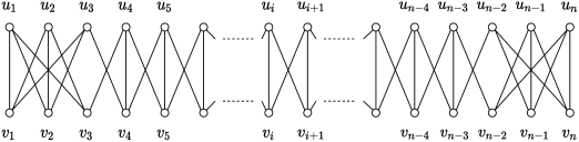
In order to prove the asymptotic value of the minimum algebraic connectivity, we need to know the structure of the extremal graph. For , let be a cubic bipartite graph on vertices, as shown in Figure 1. We show that is the unique extremal graph.
Theorem 1.4.
Among all connected cubic bipartite graphs, is the unique graph with the minimum algebraic connectivity, where
A matching in a graph is a set of edges such that no two of which have a common vertex. A matching is perfect if every vertex of the graph is incident to an edge of the matching. In [26], Horak and Kim studied the number of perfect matchings in cubic graphs. For cubic bipartite graphs, they provided the maximum number of perfect matchings by the Fibonacci numbers.
Theorem 1.5.
([26]) For , is the unique graph with the maximum number of perfect matchings among all connected cubic bipartite graphs on vertices.
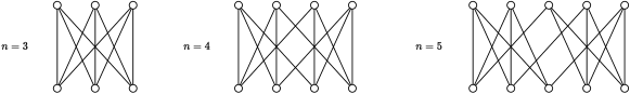
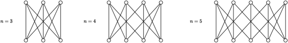
It is worth mentioning that, for small , the extremal graphs with minimum algebraic connectivity and maximum number of perfect matchings are exhibited in Figures 2 and 3, respectively. For simplicity of the statement, we omit these small cases in Theorems 1.4 and 1.5.
Combining Theorems 1.4 and 1.5, we obtain immediately a spectral characterization for cubic bipartite graphs with maximum number of perfect matchings.
Theorem 1.6.
Among all connected cubic bipartite graphs on at least vertices, the graph attains maximum number of perfect matchings if and only if it has the minimum algebraic connectivity (spectral gap).
The rest of the paper is organized as follows. In the next section, some properties on the Fiedler vector are obtained, and the unique connected cubic bipartite graph with minimum algebraic connectivity is determined. Moreover, we provide the proof of Theorem 1.4. The proof of Theorem 1.3 is presented in Section 3. In the final section, we give equivalent results of Theorems 1.3 and 1.4 for the spectral gap.
2 Extremal graph with minimum algebraic connectivity
Let us recall some basic properties for the Laplacian eigenvalues of graphs. Let be a graph on vertices with minimum degree . Clearly, 0 is the smallest Laplacian eigenvalue of , and all ones vector is the corresponding eigenvector. Let be an eigenvector of corresponding to the algebraic connectivity . Such an eigenvector is also called the Fiedler vector of . For any vertex , the entry of corresponding to is denoted by . Note that . According to Courant-Fischer Theorem, one can see that
| (1) |
It is well-known that the algebraic connectivity is not greater than the minimum degree, that is,
Denote by the complement of . The Laplacian spectral radius of is written as . Obviously, the maximum degree of is . A famous lower bound for the Laplacian spectral radius is
with equality if and only if . If is connected, then , and so . Note also that and satisfy
Combining the above facts, one can see that
| (2) |
if is connected.
Given a graph , let be four distinct vertices in satisfying the following condition:
Clearly, the induced subgraph is isomorphic to . Then we say that is a pair of independent edges.
Lemma 2.1.
Let be a connected graph with a pair of independent edges . Suppose that is a Fiedler vector of and . Let be a connected graph obtained from by deleting edges and adding edges . If and , then .
Proof.
We may assume that is a unit Fiedler vector. If , then
where the last inequality holds since and . According to (1), it follows that
as required.
In the following, we assume that . Suppose that . Then the minimum degree of is at most . It follows from (2) that . We construct a new vector such that
It is easy to see that
hence . Set and . In the graph , the neighborhood of and are and , respectively. Then we obtain that
Moreover, according to , we have
Since , it follows that
Therefore, we obtain that
where the last inequality follows from the fact . Note that
According to (1), it follows that
This completes the proof. ∎
The following useful lemma on the Fiedler vector is due to Fiedler [10].
Lemma 2.2.
([10]) Let be a connected graph with a Fiedler vector . For any , let
Then the subgraphs induced by and are connected.
Let be the set of all connected cubic bipartite graphs on vertices. A graph in is called extremal if it has the minimum algebraic connectivity. The aim of this section is to determine the extremal graph in . Suppose that is an extremal graph in with bipartition . Let be a pair of independent edges in with and . We define four vertex sets , , and .
The following lemmas present some properties on the Fiedler vector of the extremal graph .
Lemma 2.3.
Let be an extremal graph in . Suppose that is a pair of independent edges in as defined above.
Let be a unit Fiedler vector of . If and , then the following statements hold.
(P1) contains no cut edge.
(P2) is an edge cut.
(P3) and .
(P4) .
(P5) .
Proof.
If there exists a cut edge in , then a component of has the degree sequence . Note that such a component is also a bipartite graph. However, the sequence cannot be the degree sequence of any bipartite graph, hence there is no cut edge in , and so (P1) holds.
We claim that the graph must be disconnected. Otherwise, if is connected, then Lemma 2.1 shows that the algebraic connectivity of is less than the algebraic connectivity of , a contradiction.
If is connected, then the graph is clearly connected, a contradiction. Therefore, is an edge cut. So (P2) holds.
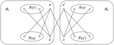
According to (P1) and (P2), there are exactly two components in , say and . If (or ) contains only one vertex of , then there is a cut edge in , contradicting (P1). Thus, . If and belong to the same component, then and are included in the other component. However, in this case, the graph is still connected, a contradiction. Therefore, without loss of generality, we may assume that and . In view of the above assumption, the local structure of is exhibited in Figure 4. It is easy to see that and , and (P3) follows.
Choose a vertex . Clearly, is also a pair of independent edges in . Let be a path in . Consider the graph . In this graph, the vertices are connected by the path . Hence is connected. If , then it follows from Lemma 2.1 that the algebraic connectivity of is less than the algebraic connectivity of , a contradiction. Therefore, we obtain that , and so . A similar argument, using Lemma 2.1, yields that , and . Now statements (P4) and (P5) hold directly. ∎
Lemma 2.4.
Let be an extremal graph in . Suppose that and are two nonadjacent vertices belonging to different parts of .
Let be three vertices such that , and .
(1) If and ,
then is adjacent to both and .
(2) If and ,
then is adjacent to both and .
Proof.
Lemma 2.5.
Let be an extremal graph with the bipartition . If is a vertex in such that , then .
Proof.
Suppose that and . Let be a vertex in with . We only need to show that . We prove it by contradiction. Suppose that . Since the degree of is 3, then there is a vertex such that and . Clearly, is a pair of independent edges in . Since and , by Lemma 2.3(P4), we have . which contradicts the maximality of . Hence the result follows. ∎
Similar to the proof of Lemma 2.5, we can obtain the following result.
Lemma 2.6.
Let be an extremal graph with the bipartition . If is a vertex in such that , then .
In the following, we determine the structure of the extremal graph . For , it is easy to determine the extremal graphs by a directly computation. As mentioned in Section 1, the extremal graphs for small are presented in Figure 2. Next we only need to consider the case , that is, there are at least 12 vertices in . Suppose that the bipartition of is , where and .
Let be a unit Fiedler vector of . According to Lemmas 2.5 and 2.6, after a relabeling of the vertices of , we may assume that the vertices satisfying:
-
(1)
,
-
(2)
,
-
(3)
,
-
(4)
.
Let be a vertex subset of the extremal graph . We denote by the sum of the entries of the Fiedler vector corresponding to the vertices in , that is,
The following basic property on the Fiedler vector is useful.
Lemma 2.7.
Let and be any two vertices in . Then
(i) if and only if ,
(ii) if and only if .
Proof.
Note that It follows that
that is,
Similarly, we can obtain
According to (2), we have , and hence the result follows immediately. ∎
In order to determine the structure of the extremal graph , we need to establish the adjacency rule of the first six vertices .
Lemma 2.8.
and .
Proof.
If , then
Since , it follows that . This implies that the vector is non-positive, which contradicts the definition of the Fiedler vector. It follows that . Similarly, since . ∎
Lemma 2.9.
and .
Proof.
Since these two inequalities can be proved by the same approach, we only present the proof of the inequality .
We establish the inequality by contradiction. Suppose that . Hence . Note that . Since and , we have . Moreover, one can see that
and so . Hence .
In summary, we obtain that
Next we will divide the proof into the following two cases.
Case 1. , i.e., .
If , then
This implies that , and it follows from Lemma 2.7 that , contradicting the assumption that . Thus, . If , then
contradicting the assumption that . Hence . It follows that , and so .
Subcase 1.1. .
In this case, and . Suppose that , where . Note that . Let with . Since , we have , hence .
Assume that . Hence is a pair of independent edges. Since and , it follows from Lemma 2.3 that , contradicting the fact . Therefore, we have . A similar argument shows that . Hence .
Let with and . Note that . It follows from Lemma 2.7 that , which implies that . Since there are at least 12 vertices in , the vertex cannot be adjacent to both and . We may assume that . Clearly, is a pair of independent edges. Since and , by Lemma 2.3, we obtain that . But this contradicts the fact .
Subcase 1.2. .
Without loss of generality, we may assume that and . Then we have . Suppose that , where . Since , it follows from Lemma 2.7 that , hence .
Assume that with . Clearly, and . If , then
By Lemma 2.7, it follows that , a contradiction. Thus, we have . One can see that is a pair of independent edges. Note that and . According to Lemma 2.3, it follows that
Thus,
Since , we have
Hence it follows from Lemma 2.7 that , a contradiction.
Case 2. , i.e., .
Consider the neighbours of and . Note that and . This shows that , and so . Moreover, since , by Lemma 2.7, we have . Therefore, the vertex cannot be adjacent to both and . It follows that . Similarly, we can also obtain that .
Subcase 2.1. Either or .
Suppose first that . Recall that . Without loss of generality, we may assume that where .
We claim that . If not, suppose that there is a vertex , where , such that . Thus is a pair of independent edges in . Note that and . According to Lemma 2.3, we obtain that . But, in this case, is the only one vertex with , then we obtain a contradiction.
Suppose that . We may assume that with . If , then the subgraph of induced by vertices is a cubic bipartite graph, this contradicts that contains at least 12 vertices. Hence . Let be the neighbour of other than and . Clearly, and . Since , we have , and so . It follows that is a pair of independent edges in . Since and , by Lemma 2.3, we obtain that . However, the vertex is adjacent to both and , a contradiction.
Suppose now that . Let with and . Since , it follows that . Let . Moreover, since , by Lemma 2.7, we have . This implies that . Suppose that . If , then is a pair of independent edges in . Clearly, and . According to Lemma 2.3, we have , this leads to , a contradiction. Therefore, we obtain that . Similarly, one can see that is also adjacent to . It follows that and are adjacent to all vertices in . On the other hand, since the degree of any vertex in is 3, we can see that , that is, is the only one vertex in . This leads to that must be adjacent to . But, in this case, the subgraph of induced by vertices is a cubic bipartite graph, which contradicting the fact that has at least 12 vertices.
In summary, we always obtain a contradiction if . Indeed, by a similar argument, one can also obtain a contradiction when .
Subcase 2.2. .
Lemma 2.10.
.
Proof.
Suppose to the contrary that . To obtain a contradiction, we first prove the following claim.
Claim 1. and .
Proof of Claim 1..
We first show that . Suppose that . Since , we have . According to Lemma 2.9, it follows that and .
If , then we assume that where and . Let with and . Note that and . By Lemma 2.4, we obtain that , , and . One can see that . Choose a vertex . Clearly, and . It follows from Lemma 2.4 that and . Then we obtain that , which implies that the degree of is at least 4, a contradiction.
Assume that . One can see that . Let be a vertex in with . Clearly, is a pair of independent edges in . Note that and . According to Lemma 2.3, we obtain that , which contradicts the fact that is adjacent to both and .
Hence . A similar argument shows that . This completes the proof of Claim 1. ∎
It follows from Claim 1 that and . Recall that . According to the adjacency relation of and , we divide the proof into the following two cases.
Case 1. .
Suppose that where . Since , it follows from Lemma 2.7 that , hence . If , then . By Lemma 2.7, we have , a contradiction. Hence .
Subcase 1.1. .
Thus we may assume that with . Since and , Lemma 2.4 shows that is adjacent to both and . If , then the subgraph induced by is a cubic bipartite graph, which contradicts the fact that there are at least 12 vertices in . Hence . One can see that is a pair of independent edges in . Since , by Lemma 2.7, we obtain that . Note also that . Using Lemma 2.3, it follows that . But this contradicts the fact that is adjacent to both and .
Subcase 1.2. .
Suppose that with . According to Lemma 2.4, it follows that both and . Suppose that where . Since and , we obtain that
It follows from Lemma 2.7 that . This implies that . If , then . Since , it follows that
By Lemma 2.7, we obtain that , a contradiction. Hence . Clearly, is a pair of independent edges in . Since and , using Lemma 2.3, we obtain that . Thus we obtain a contradiction since is a common neighbour of and .
Case 2. .
Arguing similarly to that in Subcase 1.2, we can also obtain a contradiction if . So we assume that . Suppose that and , where and . We claim that . If not, it follows that . Thus . By Lemma 2.7, we obtain , contradicting Claim 1. This implies that . Similarly, one can also obtain .
We claim that . Suppose that . If , then it follows from Lemma 2.4 that , a contradiction. Hence . Similarly, one can see that . It follows that
By Lemma 2.7, we have , a contradiction. Therefore .
Suppose now without loss of generality that . Lemma 2.8 shows that and . Since , we can choose a real number such that . It follows from Lemma 2.2 that is connected. On the other hand, according to the above adjacency relations, it is easy to see that is a vertex cut of , and the vertices and belong to the different components in . This implies that any path from to must pass through either or . Note that and , as . Then we obtain that there are no paths from to in the subgraph induced by , a contradiction to the connectedness of . The proof is completed. ∎
Lemma 2.11.
.
Proof.
Suppose to the contrary that . Let with . To obtain the contradiction, we will consider the following cases.
Case 1. .
It is easy to see that . If not, and have the same neighbours, thus Lemma 2.7 leads to that , contradicting Lemma 2.9. Suppose that , where . We claim that is adjacent to both and . Note that and . If , then Lemma 2.4 shows that is adjacent to both and . If , then
Then it follows from Lemma 2.7 that . Again, Lemma 2.4 shows that is adjacent to both and . Hence . Suppose that where and . Since , by Lemma 2.7, we have , hence . Note also that . Using Lemma 2.4, we obtain that and . Thus the subgraph of induced by is a cubic bipartite graph, a contradiction.
Case 2. .
Suppose that with .
Subcase 2.1. .
We first prove that . Suppose to the contrary that . Then forms a pair of independent edges in . Clearly, and . If either or , then it follows form Lemma 2.3 (P3) that , which contradicts the fact that . Hence and . Since , it follows from Lemma 2.7 that , a contradiction with Lemma 2.9. Hence . Similarly, one can obtain that .
If , then the subgraph of induced by is a cubic bipartite graph, a contradiction. This implies that . Obviously, is a pair of independent edges in . Note that and . Since , it follows from Lemma 2.7 that . Using Lemma 2.3 (P3), we have . But is a common neighbour of and , a contradiction again.
Subcase 2.2. .
Let with . We will show that is adjacent to both and . Note that and . If , then Lemma 2.4 shows that and . Assume that . Then we have
According to Lemma 2.7, it follows that . Combining with Lemma 2.9, we obtain that , hence . Using Lemma 2.4, we also obtain that and .
We may assume that with . Clearly, and . Note that and . If , then Lemma 2.4 shows that and . Suppose now that . Hence
It follows from Lemma 2.7 that . According to Lemma 2.4, one can see that and .
Therefore, . But this contradicts the degree of . ∎
Lemma 2.12.
.
Proof.
Lemma 2.13.
and .
Proof.
Lemma 2.14.
and .
Proof.
Now there is only one undetermined neighbour of . We may assume that with . It suffices to show that .
Therefore, arguing similarly to that in the proof of Lemma 2.14, we obtain the following lemma.
Lemma 2.15.
and .
Let us consider the adjacency relations for the subsequent vertices. For a given positive integer , we define
Lemma 2.16.
For any , the following statements hold:
(1) , and ,
(2) and .
Proof.
We prove the result by induction on . Consider the case . Lemmas 2.14 and 2.15 show that
It suffices to show that . Suppose to the contrary that . Note that
According to Lemma 2.4, it is easy to see that every vertex in is adjacent to every vertex in . Therefore, the subgraph of induced by is a cubic bipartite graph. This implies that contains only four vertices. But this contradicts the fact . Hence . The result holds for .
Suppose now that . By the induction hypothesis, we obtain that
We first prove that and . Let be the neighbour of with . It suffices to prove that . Suppose to the contrary that there is a vertex such that , where and . In this case, it is to see that . Clearly, , which implies that . By Lemma 2.4, the vertex is adjacent to all vertices in , and hence the degree of is at least 4, a contradiction. Therefore, it follows that and . Similarly, we can show that and .
It remains to prove that . Assume that . Then one can see that , and . Since and , by Lemma 2.4, every vertex in is adjacent to every vertex in . It is easy to see that the subgraph of induced by is a cubic bipartite graph. This implies that there are only four vertices in , which yields that . But this contradicts the fact . Hence and the proof is completed. ∎
In summary, according to Lemmas 2.10, 2.11, 2.12 and 2.16, we determine the adjacency relations of all vertices in . Now we are ready to prove Theorem 1.4.
Proof of Theorem 1.4.
If , then must be adjacent to a vertex . Hence . Lemma 2.16 shows that . Morevoer, since , by Lemma 2.4, the vertex is adjacent to all vertices in . This implies that the degree of is equal to 4, a contradiction. Hence . Similarly, one can see that .
When , the graph cannot be a cubic bipartite graph. If , it is easy to see that is clearly isomorphic to , and the result follows. ∎
3 Algebraic connectivity of the extremal graph
In this section, we consider the asymptotic value for the algebraic connectivity of the extremal graph. As mentioned in Section 2, is the unique cubic bipartite graph with minimum algebraic connectivity. Label the vertices of as shown in Figure 1. Before proceeding further, let us present the following property for the Fiedler vector of
Lemma 3.1.
The extremal graph has a Fiedler vector such that for any .
Proof.
According to Lemma 2.8, for the extremal graph , there is a Fiedler vector such that and . Let and , where . Construct a vector on the vertices of such that and for . According to the symmetry of , it is easy to see that is also a Fiedler vector of . Let us consider a new vector . Since and , then we obtain that . Clearly, is a nonzero vector since . Hence is also a Fiedler vector of . Moreover, one can see that for . Obviously is a Fiedler vector of with the desired property. ∎
Let denote a path on vertices. The Laplacian spectrum of consists of the numbers , where (see, e.g., [4]). Clearly, . Note also that is a tridiagonal matrix. The eigenvalues and eigenvectors of a certain tridiagonal matrix were discussed in [37]. Indeed, applying the conclusions in [37], one can also derive all eigenvalues and eigenvectors of . In particular, the Fiedler vector of is skew symmetry. To make the paper self-contained, we give a proof by using Lemma 2.2.
Lemma 3.2.
The Fiedler vector of is skew symmetry.
Proof.
Let be a unit Fiedler vector of . Suppose that . Without loss of generality, we may assume that .
We first claim that . Suppose that . Since , then we have . Furthermore, one can see that since . Repeating this process, we will finally obtain a zero vector, a contradiction.
Let us consider another vector on the vertices of , where for . Clearly, the vector is obtained from by exchanging the entries corresponding to vertices and . According to the symmetry of , is also a Fiedler vector of . Recall that is a simple eigenvalue of . Hence .
If , then . Since , then the vector contains a negative entry. Suppose that with . Let . Lemma 2.2 shows that the subgraph induced by is connected. But this is impossible since . It follows that . Hence for , as required. ∎
Theorem 3.3.
The algebraic connectivity of is .
Proof.
We first prove that is a lower bound for . Let be a Fiedler vector of satisfying the property in Lemma 3.1. Hence for any . Note that
Expanding the right side of the above equality, we have
| (3) |
Let be a path on vertices. According to (1), it follows that
| (4) |
Combining (3) and (4), we obtain . It is well-known that . Thus we obtain that
which implies the desired lower bound.
Now we show that is an upper bound for . Let be a path on vertices. Assume that is a Fiedler vector of . Set for . Construct a new vector on vertices of as follows:
According to Lemma 3.2, it is easy to see that . By (1), we obtain that
| (5) |
On the other hand, since is a Fiedler vector of , it follows that
| (6) |
Combining (5) and (6), we obtain
Therefore, . ∎
4 Concluding remarks
In this paper, we determine the unique graph with minimum algebraic connectivity among all connected cubic bipartite graphs, and obtain the asymptotic value of the minimum algebraic connectivity. For any -regular graph , its diagonal martix of vertex degrees is , where is the identity matrix. According to the definition of Laplacian matrix, one can see that the Laplacian matrix and adjacency matrix of satisfy
The difference between the two largest eigenvalues of is called the spectral gap of . According to the above equation, one can see that the spectral gap of is equal to its algebraic connectivity. Using this fact, Theorems 1.3 and 1.4 imply the following results directly.
Theorem 4.1.
The minimum spectral gap of connected cubic bipartite graphs on vertices is .
Theorem 4.2.
Among all connected cubic bipartite graphs with at least 12 vertices, is the unique graph with minimum spectral gap.
Lemma 2.1 establishes a transformation which strictly decreases the algebraic connectivity. We remark that this transformation also works for general -regular bipartite graphs. Then it is natural to investigate the minimum algebraic connectivity (spectral gap) of -regular bipartite graphs for . Based on our observations, we think that the extremal graph will be path-like when is sufficiently large. In Theorem 1.6, we present a spectral characterization for cubic bipartite graphs with maximum number of perfect matchings. For general -regular bipartite graphs, it is also interesting to find the spectral characterization for the extremal graphs with maximum number of perfect matchings.
Acknowledgements
The research of Ruifang Liu is supported by National Natural Science Foundation of China (Nos. 11971445 and 12171440) and Natural Science Foundation of Henan Province (No. 202300410377). The research of Jie Xue is supported by National Natural Science Foundation of China (No. 12001498) and China Postdoctoral Science Foundation (No. 2022TQ0303).
References
References
- [1] M. Abdi, E. Ghorbani, Quartic graphs with minimum spectral gap, J. Graph Theory, 2022, DOI:10.1002/jgt.22867.
- [2] M. Abdi, E. Ghorbani, W. Imrich, Regular graphs with minimum spectral gap, European J. Combin. 95 (2021) 103328.
- [3] C. Brand, B. Guiduli, W. Imrich, The characterization of cubic graphs with minimal eigenvalue gap, Croat. Chem. Acta 80 (2007) 193–201.
- [4] A. Brouwer, W. Haemers, Spectra of graphs, Springer, New York, 2012.
- [5] D. Cardoso, C. Delorme, P. Rama, Laplacian eigenvectors and eigenvalues and almost equitable partitions, European J. Combin. 28 (2007) 665–673.
- [6] W. Cames van Batenburg, Minimum maximal matchings in cubic graphs. Electron. J. Combin. 29 (2022) #2.36.
- [7] S. Das, A. Pokrovskiy, B. Sudakov, Isomorphic bisections of cubic graphs, J. Combin. Theory Ser. B 151 (2021), 465–481.
- [8] N.M.M. de Abreu, Old and new results on algebraic connectivity of graphs, Linear Algebra Appl. 423 (2007) 53–73.
- [9] M. Fiedler, Algebraic connectivity of graphs, Czechoslovak Math. J. 23 (1973) 298–305.
- [10] M. Fiedler, A property of eigenvectors of nonnegative symmetric matrices and its application to graph theory, Czechoslovak Math. J. 25 (1975) 619–633.
- [11] S. Fallat, S. Kirkland, Extremizing algebraic connectivity subject to graph theoretic constraints, Electron. J. Linear Algebra 3 (1998) 48–74.
- [12] S. Fallat, S. Kirkland, S. Pati, Minimizing algebraic connectivity over connected graphs with fixed girth, Discrete Math. 254 (2002) 115–142.
- [13] R. Grone, R. Merris, Ordering trees by algebraic connectivity, Graphs Combin. 6 (1990) 229–237.
- [14] X. Gu, M. Liu, A tight lower bound on the matching number of graphs via Laplacian eigenvalues, European J. Combin. 101 (2022) 103468.
- [15] J. Guo, A conjecture on the algebraic connectivity of connected graphs with fixed girth, Discrete Math. 308 (2008) 5702–5711.
- [16] J. Guo, W. Shiu, J. Li, The algebraic connectivity of lollipop graphs, Linear Algebra Appl. 434 (2011) 2204–2210.
- [17] S. Guo, R. Zhang, G. Yu, Hamiltonian graphs of given order and minimum algebraic connectivity, Linear Multilinear Algebra 66 (2018) 459–468.
- [18] B. Guiduli, The structure of trivalent graphs with minimal eigenvalue gap, J. Algebraic Combin. 6 (1997) 321–329.
- [19] F. Kirchhoff, Über die Auflösung der Gleichungen, auf welche man bei der Untersuchung der linearen Verteilung galvanischer Ströme geführt wird, Ann. Phys. Chem. 72 (1847) 497–508.
- [20] S. Kirkland, J. Molitierno, B. Shader, On graphs with equal algebraic and vertex connectivity, Linear Algebra Appl. 341 (2002) 45–56.
- [21] S. Kirkland, I. Rocha, V. Trevisan, Algebraic connectivity of -connected graphs, Czechoslovak Math. J. 65 (2015) 219–236.
- [22] T. Kolokolnikov, Maximizing algebraic connectivity for certain families of graphs, Linear Algebra Appl. 471 (2015) 122–140.
- [23] J. Li, J. Guo, W. Shiu, The smallest values of algebraic connectivity for unicyclic graphs, Discrete Appl. Math. 158 (2010) 1633–1643.
- [24] S. Hedetniemi, D. Jacobs, V. Trevisan, Domination number and Laplacian eigenvalue distribution, European J. Combin. 53 (2016) 66–71.
- [25] Y. Higuchi, Y. Nomura, Spectral structure of the Laplacian on a covering graph, European J. Combin. 30 (2009) 570–585.
- [26] P. Horak, D. Kim, Connected cubic graphs with the maximum number of perfect matchings, J. Graph Theory 99 (2022) 671–690.
- [27] K. Knauer, P. Valicov, Cuts in matchings of 3-connected cubic graphs, European J. Combin. 76 (2019) 27–36.
- [28] E. Máčajová, M. Škoviera, Cubic graphs that cannot be covered with four perfect matchings, J. Combin. Theory Ser. B 150 (2021) 144–176.
- [29] E. Máčajová, M. Škoviera, Martin Perfect matching index versus circular flow number of a cubic graph, SIAM J. Discrete Math. 35 (2021) 1287–1297.
- [30] R. Merris, Laplacian matrices of graphs: a survey, Linear Algebra Appl. 197/198 (1994) 143–176.
- [31] R. Merris, A survey of graph Lpalacians, Linear Multilinear Algebra 39 (1995) 19–31.
- [32] B. Mohar, Laplace eigenvalues of graphs-a survey, Discrete Math. 109 (1992) 171–183.
- [33] R. Olfati-Saber, R. Murray, Consensus problems in networks of agents with switching topology and time-delays, IEEE Trans. Autom. Control 49 (2004) 1520–1533.
- [34] K. Ogiwara, T. Fukami, N. Takahashi, Maximizing algebraic connectivity in the space of graphs with a fixed number of vertices and edges, IEEE Trans. Control Netw. Syst. 4 (2017) 359–368.
- [35] J. Shao, J. Guo, H. Shan, The ordering of trees and connected graphs by algebraic connectivity, Linear Algebra Appl. 428 (2008) 1421–1438.
- [36] H. Wang, R. Kooij, P. Mieghem, Graphs with given diameter maximizing the algebraic connectivity, Linear Algebra Appl. 433 (2010) 1889–1908.
- [37] A. Willms, Analytic results for the eigenvalues of certain tridiagonal matrices, SIAM J. Matrix Anal. Appl. 30 (2008) 639–656.
- [38] Y. Wu, G. Yu, J. Shu, Graphs with small second largest Laplacian eigenvalue, European J. Combin. 36 (2014) 190–197.
- [39] J. Xue, H. Lin, J. Shu, The algebraic connectivity of graphs with given circumference, Theoret. Comput. Sci. 772 (2019) 123–131.
- [40] S. Zhang, Q. Zhao, H. Liu, The algebraic connectivity of graphs with given stability number, Electron. J. Linear Algebra 32 (2017) 184–190.
- [41] X. Zhang, Graphs with fourth Laplacian eigenvalue less than two, European J. Combin. 24 (2003) 617–630.