Doubly-Optimistic Play for Safe Linear Bandits

Abstract

The safe linear bandit problem (SLB) is an online approach to linear programming with unknown objective and unknown round-wise constraints, under stochastic bandit feedback of rewards and safety risks of actions. We study aggressive doubly-optimistic play in SLBs, and their role in avoiding the strong assumptions and poor efficacy associated with extant pessimistic-optimistic solutions.

We first elucidate an inherent hardness in SLBs due the lack of knowledge of constraints: there exist ‘easy’ instances, for which suboptimal extreme points have large ‘gaps’, but on which SLB methods must still incur $\Omega(\sqrt{T})$ regret and safety violations due to an inability to refine the location of optimal actions to arbitrary precision. In a positive direction, we propose and analyse a doubly-optimistic confidence-bound based strategy for the safe linear bandit problem, DOSLB, which exploits supreme optimism by using optimistic estimates of both reward and safety risks to select actions. Using a novel dual analysis, we show that despite the lack of knowledge of constraints, DOSLB rarely takes overly risky actions, and obtains tight instance-dependent $O(\log^{2}T)$ bounds on both efficacy regret and net safety violations up to any finite precision, thus yielding large efficacy gains at a small safety cost and without strong assumptions. Concretely, we argue that algorithm activates noisy versions of an ‘optimal’ set of constraints at each round, and activation of suboptimal sets of constraints is limited by the larger of a safety and efficacy gap we define.

1 Introduction

Stochastic linear bandits form a canonical setting to probe the use of structure to navigate the exploration-exploitation question in large action spaces. In a series of rounds, indexed by $t$, a learner ‘plays’ an action $x_{t}\in\mathcal{S}\subset\mathbb{R}^{d},$ where $\mathcal{S}$ is a bounded polytope, and observes noisy feedback of the form $\langle\theta,x_{t}\rangle+w_{t},$ where $\theta$ is a latent parameter. The goal of the learner is to maximise cumulative reward over the course of the play $\sum\langle\theta,x_{t}\rangle,$ ideally ensuring that this is close to $\sum\langle\theta,x^{*}\rangle,$ where $x^{*}$ is a solution to the underlying linear program (LP) $\max\langle\theta,x\rangle:x\in\mathcal{S}$. This problem thus encompasses an online approach to LP with noisy zeroth-order feedback, and has a plethora of applications accruing from the ubiquity of both LPs and bandit settings. Of course, most such application domains also impose constraints on the actions that may be taken. Usually, the set $\mathcal{S}$ plays the role of enforcing these constraints. However, in the standard bandit literature, this set is assumed to be known a priori, which is an unrealistic assumption in a variety of important cases.

Round-Wise Latent Constraints.

The Safe-Linear Bandit (SLB) problem addresses the above lacuna through round-wise enforcement of latent linear constraints: given constraint levels $\alpha^{i},$ we attempt to enforce that in each round, $\langle a^{i},x_{t}\rangle\leq\alpha^{i},$ for unknown $a^{i}$, using noisy observations of constraint levels, $\langle a^{i},x_{t}\rangle+w^{i}_{t},$ to enable learning. The following example motivates this study.

Drug Trials (Whitehead; 1983). Consider the case of treating patients with cocktails of some $d$ drugs over the course of a trial. In such a scenario, both the efficacy and the side-effects of a cocktail are a priori undetermined. Here, we may model the efficacy of the cocktail $x$ as $\langle\theta,x\rangle,$ and each $\langle a^{i},x\rangle$ may model the extent of side-effects on particular systems of the body, for instance, the drop in a heart- or liver-function score. The constraint levels $\alpha^{i}$ represent score drops that are deemed safe by domain experts. Since these scores and the efficacy can be measured, we obtain feedback of the type desired, with stochasticity arising due to inter-patient variability. Naturally, we need to enforce constraints on every round, since we need to ensure that patients are treated safely.

Similar considerations apply broadly, e.g., in engineering design, one would maximise performance while ensuring that loads on each component in the system are not beyond their nominal limits, and in designing web interfaces, one may optimise revenue while limiting customer friction.

To discuss the existing approaches to this problem, and our work, let us define the cumulative efficacy regret, and net safety violation of a sequence of actions $\{x_{t}\}$ as

$$\mathscr{E}_{T}:=\sum_{t\leq T}(\langle\theta,x^{*}-x_{t}\rangle)_{+},\quad\textit{and}\quad\mathscr{S}_{T}:=\sum_{t\leq T}\max_{i}(\langle a^{i},x_{t}\rangle-\alpha_{i})_{+}.$$ (1)

Observe that by penalising the positive part of the inefficiency and violations of $x_{t}$, these metrics indeed capture the round-wise enforcement of constraints: if an effective but unsafe action is played, then it does not decrease $\mathscr{E}_{T}$, but causes an increase in $\mathscr{S}_{T}$.

The majority of extant solutions to the SLB problem study hard constraint satisfaction, i.e., enforcing that $\mathscr{S}_{T}=0$ with high probability, and take the ‘pessimistic-optimistic’ (PO) approach (Amani et al.; 2019, Moradipari et al.; 2021, Pacchiano et al.; 2021, Bernasconi et al.; 2022). While these safety guarantees are strong, PO methods carry significant costs, since they $\mathrm{(i)}$ require, as input, an explicit nontrivially sized region that is known a priori to be safe, which is a strong assumption, and $\mathrm{(ii)}$ only provide efficacy guarantees of the form $\mathscr{E}_{T}=O((M^{\mathsf{s}})^{-1}\sqrt{T}),$ where $M^{\mathsf{s}}$ is a measure of the size of this safe region, as opposed to the $O(\log^{2}T)$ instance-dependent bounds that may be attained when the constraints are known (also see §7.2). Our paper focuses on exploring methods that improve these aspects, but at the cost of weaker ‘soft’ safety guarantees of the form $\mathscr{S}_{T}=o(T)$.

Soft constraint satisfaction: a pragmatic view.

The main justification for soft enforcement approach arises from a pragmatic consideration of constraints in practical settings. Indeed, while optimisation problems are usually formulated with given hard constraint levels, in typical applications these constraints are not quite as hard, and the underlying systems are robust to small violations of these. There are two main ways in which this robustness can arise:

• Precision of a continuous response. In drug trials, the level $\alpha^{i}$ describes the amount of decrease in a system function score that is deemed safe. However, the effect such a decrease on patient health is a continuous response, and a small increase in such a score has a practically identical effect (Katz; 2012). Similar considerations apply in the other examples above, and are bolstered by the fact that engineered systems often include wide factors of safety in component choice (NASA; 2008).

• Constraining a mean. More concretely, observe that the constraints in $\mathscr{S}_{T}$ are being enforced on the mean of the safety risks. Much like ‘pseudo-regret’ does not control the actual regret incurred, we are effectively dealing with ‘pseudo-constraints’. The stochasticity inherent in individual rounds means that typically actions that are safe in this mean sense would still lead to harmful side-effects with nontrivial chance. So long as this chance is governed by a light-tailed noise, small violations of the constraints is unlikely to increase the overall extent of side-effects very much.

Thus, in important practical situations, constraint levels can be treated softly: while we do need to ensure that constraints are not violated by too large a value in most rounds, persistent small violations, or occasional large violations are fine for the long-run operation of a system. Such behaviour is achieved by any method that ensures that $\mathscr{S}_{T}$ is small (but possibly non-zero). Our main question regards understanding the tradeoff between $\mathscr{E}_{T}$ and $\mathscr{S}_{T},$ and how much such a relaxation buys us:

What efficacy regret performance can we get while ensuring that net safety violations are small?

To answer this question, we propose and analyse a ‘doubly-optimistic’ (DO) confidence-bound based method for SLBs, DOSLB. At each $t$, DOSLB constructs a permissible set $\widetilde{\mathcal{S}}_{t}$ consisting of all actions that could plausibly be safe given the history, and selects $x_{t}\in\widetilde{\mathcal{S}}_{t}$ by maximising an optimistic reward estimate. Since $\widetilde{\mathcal{S}}_{t}$ is an outer approximation to the feasible set $\mathcal{S},$ and the method is ‘optimistic’ about both the efficacy and the safety of actions, it is doubly-optimistic.

Contributions.

We summarise our main results, one negative and one positive.

The SLB Problem is Hard. We show that for every method, there exists a ‘well-separated’ instance on which it suffers $\max(\mathscr{E}_{T},\mathscr{S}_{T})\geq\Omega(\sqrt{T})$. This means that even when the instances are nominally ‘easy’ (i.e., logarithmic regret bounds would hold if the constraints were known; §4), the SLB methods must still incur large ‘regret’. This barrier arises due to an inability to estimate locations of extreme points to precision better than $1/\sqrt{T}$, and is a fundamental hardness in the problem.

Softness Makes SLBs Easy. Under mild conditions, we show that DOSLB ensures that simultaneously $\forall\varepsilon>0,$ $\max(\mathscr{E}_{T},\mathscr{S}_{T}^{\varepsilon})=O(\log^{2}T),$ where $\mathscr{S}_{T}^{\varepsilon}:=\sum\max_{i}(\left\langle a^{i},x_{t}\right\rangle-\alpha^{i}-\varepsilon)_{+}$ represents safety violations upto $\varepsilon$-precision in the constraint levels. Thus, allowing small safety violations leads to a tremendous improvement in the efficacy regret attainable, without any prior knowledge of a large set of safe actions. We further show that in infinite precision, $\mathscr{E}_{T}=O(\log^{2}T)$ and $\mathscr{S}_{T}=\widetilde{O}(\sqrt{T}).$ In an imprecise sense, this result is shown by defining two novel measures of inefficacy and lack of safety of suboptimal actions, and showing that the play of poor actions is limited by the larger of these.

Comparison with PO methods. Note that while the first result applies also to PO methods, the second is not comparable with the bounds of the same. Indeed, the improvements in efficacy regret do (and must, due to the first result) rely on a relaxed approach to the net safety violations. Nevertheless, since play for PO methods must stay near the a priori safe region for a large time, allowing a relaxed precision for PO methods would leave them with $\Omega(\sqrt{T})$ regret on $\mathscr{E}_{T}$. The significant gain in $\mathscr{E}_{T}$ induced by DO methods raises an important point of practical interest: when small constraint violations may be accommodated, it is imperative for good performance that one uses aggressive, optimistic learning methods rather than conservative ones. We expect that this general principle has relevance beyond SLBs, and is an important design consideration for practitioners.

Technical Novelty. The main technical challenge lies in showing the second result. We argue this by taking a dual view of the actions of DOSLB. Specifically, we show that at each $t$, the action $x_{t}$ must activate noisy versions of at least $d$ constraints (known or unknown). This allows us to use sets of indices of these constraints as a source of discreteness. We exploit this by showing that these index sets admit nonzero feasibility and efficacy gaps, such that whenever $x_{t}$ activates a ‘bad’ index set, the ‘noise scale’ at $x_{t}$ must exceed the larger of these gaps, leading to a large refinement in estimates. As a consequence, we show that that in the preponderance of times, the action of DOSLB focuses on activating the ‘correct’ set of constraints—the ones that $x^{*}$ saturates.

1.1 Related Work

We briefly discuss the most pertinent related work; see §A for a detailed treatment.

The bulk of work on constrained bandits studies aggregate constraint enforcement, i.e., controlling the regret $\mathscr{R}_{T}:=\sum_{t\leq T}\left\langle\theta,x^{*}-x_{t}\right\rangle$ and aggregate violation $\mathscr{A}_{T}:=\max_{i}(\sum_{t\leq T}\left\langle a^{i},x_{t}\right\rangle-\alpha_{i})$ (Badanidiyuru et al.; 2013, 2014, Agrawal and Devanur; 2014, 2016, Agrawal et al.; 2016). Notice that while making $(\mathscr{R}_{T},\mathscr{A}_{T})$ sublinear does mean that the ergodic average, $\sum x_{t}/T,$ is safe and effective, it does not ensure that most rounds are treated safely. The distinction from round-wise enforcement is evident in that the raw inefficacy and violations are summed in the above metrics, rather than their positive parts as in $\mathscr{E}_{T},\mathscr{S}_{T}$. Due to this, may (and do) switch between playing very safe but ineffective and very unsafe but effective actions, effectively letting the learner ‘earn’ constraint violation capacity in one round, and spend it later(Pacchiano et al.; 2021, Chen et al.; 2022). While this is fine for modeling resource usage, such behaviour is inadmissible in safety-critical settings.

Aggregate constraint methods remain an active area of research, for instance, the ‘conservative bandits’ line of work (e.g. Wu et al.; 2016) enforces properties of the form $\mathscr{A}_{t}=O(\sqrt{t})$ for most $t$, and Liu et al. (2021) show that under the knowledge of a Slater parameter, one can enforce $\mathscr{A}_{t}\leq 0$ for all $t$ large enough. Similar problems have also been studied from an optimisation point of view (e.g. Yu et al.; 2017). We also note that most work on constrained MDPs is of this flavour, where the goal is to learn policies with large reward, while ensuring that over the course of the trajectory, an aggregate cost is well controlled (for example, see the recent work of Vaswani et al. (2022) and the references therein).

In contrast, we are interested in round-wise constraint enforcement, which is the natural formulation for scenarios with safety concerns. The principal bifurcation here lies in whether constraints are treated in a hard or soft way, i.e., if achieving $\mathscr{S}_{T}=0$ is a requirement for methods or not.

Hard round-wise constraint enforement is entirely encompassed by the PO approach discussed previously. We note that the a priori safe set assumption is typically structured as being given a point $x^{\mathsf{s}}$ and (implicitly) an $M^{\mathsf{s}}>0$ such that every point in a ball of radius $M^{\mathsf{s}}$ around $x^{\mathsf{s}}$ is safe. To our knowledge, this approach was first considered in linear bandits by Amani et al. (2019), using a safely-explore-and-commit strategy, and was refined by Moradipari et al. (2021) using a dynamic exploration and using Thompson Sampling for selecting actions. Pacchiano et al. (2021) also take a similar view, but lift the action space to policies (distributions over actions), and give confidence bound based methods. Bernasconi et al. (2022) study a linearised approach to tree-form SDMs, and consider similar pessimistic bounds. We also note that this hard approach has also been studied for exploration in the finite state-action MDPs, where the demand is to learn a policy with high value while ensuring that each state visited in the trajectory is safe (Turchetta et al.; 2016, Wachi and Sui; 2020, e.g.). We leave further discussion of these PO methods to §A, although we note that both the inverse dependence on $M^{\mathsf{s}}$ and dependence on $\sqrt{T}$ that appear in efficacy regret bounds achieved by these methods are necessary ( Pacchiano et al. (2021) show the former, and our Theorem 3 shows the latter).

Soft round-wise constraint enforcement is largely driven by the doubly-optimistic approach, although all such study has been limited to the discrete action space setting. Chen et al. (2022) describe Bayesian and frequentist index-based strategies with instance dependent logarithmic bounds for multi-armed bandits; Bernasconi et al. (2022) study a linearised approach to tree-form SDMs and give $O(\sqrt{T})$ guarantees on violations and efficacy regret; and Efroni et al. (2020) study episodic finite state, action, and horizon MDPs, control efficacy and soft violation (in terms of trajectories over each episode) over $T$ episodes to $O(\sqrt{T})$. Notwithstanding the fact that bandit settings are stateless, we note that the linear setting we consider is fundamentally more challenging than these finite armed settings, since in this case the extreme points of the underlying polytope are directly revealed, while in our case these need to be discovered. Further, we give a considerably more refined study of the linear setting, capturing not only the $\sqrt{T}$ upper bounds, but demonstrating that they are fundamental even if the instance is easy, and identifying structural aspects that yield logarithmic bounds under arbitrarily mild relaxations.

Pure Exploration. We briefly discuss the pure-exploration version of safe bandit problems. Typically, these methods aim to recover arms that are both nearly-safe and nearly-optimal, in a PAC sense. Katz-Samuels and Scott (2019) study this quesiton for finite-armed bandits, and Wang et al. (2022) extend this study under a structured multi-armed bandit setting where each arm has a continuous parameter that must be selected, and monotonically affects reward and safety of the arm. Most pertinently, Camilleri et al. (2022) recently study best feasible arm identifaction in the linear bandit setting with the same structure as us, although they assume that the set of possible actions is finite and known a priori. It is interesting to note that even in the identification setting, where safety is not enforced during learning, methods that can identify good arms quickly can only give guarantees of safety up to a given precision. This complements our observations in the regret setting.

2 Problem Setup

For naturals $a\leq b$, let $[a:b]:=\{a,\dots,b\}.$ $\left\langle\cdot,\cdot\right\rangle$ and $\|\cdot\|$ denote the inner-product and $\ell_{2}$-norm in $\mathbb{R}^{d}$ respectively, and for a matrix $V\prec 0$, $\|z\|_{V}:=\sqrt{\left\langle z,Vz\right\rangle}$. For a $p\times q$ matrix $M$, and a set $\mathfrak{S}\subset[1:p],$ $M(\mathfrak{S})$ denotes the $|\mathfrak{S}|\times q$ submatrix of $M$ preserving rows indexed in $\mathfrak{S}$.

Setting. The SLB problem is parameterised by an objective vector $\theta$, $U$ unknown constraint vectors $\{a^{i}\}_{i\in[1:U]}$, and $K$ known constraint vectors $\{b^{j}\}_{j\in[1:K]}$, all in $\mathbb{R}^{d}$; and constraint levels $\{\alpha^{i}\}_{i\in[1:U]},\{\beta^{j}\}_{j\in[1:K]}$. These define the principal linear program of relevance,

$$\max_{x\in\mathbb{R}^{d}}\left\langle\theta,x\right\rangle\text{s.t. }Ax\leq\alpha,Bx\leq\beta$$

where the matrices $A,B$ and vectors $\alpha,\beta$ stack the linear constraints. The known constraints $Bx\leq\beta$ should be thought of as arising from pre-determined hard limits on $x$. We assume that these form a bounded polytope, and the above program is feasible, and admits a unique optimum $x^{*}$. The levels $\alpha,\beta,$ and the matrix $B$ are revealed to the learner, while the objective $\theta$ and the unknown constraints $A$ are hidden. We denote the feasible set as $\mathcal{S}:=\{x:Ax\leq\alpha,Bx\leq\beta\}.$

Play. The problem proceeds in rounds, indexed by $t$. For each $t$, the learner chooses an action $x_{t}\in\mathcal{X}:=\{x\in\mathbb{R}^{d}:Bx\leq\beta\},$ and receives the reward feedback $r_{t}$ and safety feedback $\{s_{t}^{i}\}_{i\in[1:U]}$

$$r_{t}=\left\langle\theta,x_{t}\right\rangle+w_{t}^{0},\quad\textit{and}\quad s_{t}^{i}=\left\langle a^{i},x_{t}\right\rangle+w_{t}^{i},$$

where the various $w_{t}^{i}$ are each marginally a conditionally centred sub-Gaussian noise, which need not be independent across $i$. The information set of the learner at time $t$ is $\mathcal{H}_{t-1}:=\{(x_{\tau},r_{\tau},\{s^{i}_{\tau}\}_{i\in[1:U]})_{\tau<t}\},$ and $x_{t}$ must be adapted to the filtration induced by $\mathcal{H}_{t-1}$. The matrix $X_{1:t}=[x_{1},\dots,x_{t}]^{\top}$ and the vectors $R_{1:t}=[r_{1},\dots,r_{t}]^{\top},S^{i}_{1:t}=[s^{i}_{1},\dots,s^{i}_{t}]^{\top}$ arise by stacking the action and feedback.

Metrics. We are interesting in controlling the cumulative Efficacy Regret and the Safety Violations, defined previously in (1). We observe again that penalising only the positive part of the round-wise inefficiency or safety violations is critical for these quantities to have relevance to the SLB setting, and particularly serves to exclude inter-round tradeoff of safety violations.

Assumptions. We conclude by noting standard assumptions due to Abbasi-Yadkori et al. (2011).

1. Boundedness: $\|\theta\|\leq 1,\|a^{i}\|\leq 1$ for all $i$, and $\{Bx\leq\beta\}\subset\{\|x\|\leq 1\}.$

2. SubGaussian Noise: $\forall t,i$ the $w_{t}^{i}$ are conditionally centred and $1$-subGaussian given $\mathcal{F}_{t}:=\sigma(\mathcal{H}_{t-1},x_{t}),$ i.e.,

   $$\forall t,i,\mathbb{E}[w_{t}^{i}|\mathcal{F}_{t}]=0,\forall\lambda,\mathbb{E}[\exp(\lambda w_{t}^{i})|\mathcal{F}_{t}]\leq\exp(\lambda^{2}/2).$$

All subsequent results should be taken to hold only under the above. See §B.1 for more details.

3 A Doubly Optimistic Algorithm for Safe Linear Bandits

The optimism principle is broadly successful in bandit problems (Lattimore and Szepesvári; 2020), and in particular for stochastic linear bandits (Dani et al.; 2008, Abbasi-Yadkori et al.; 2011). The prototypical method for this is the ‘OFUL’ algorithm, which constructs confidence sets $\mathcal{C}_{t}^{0}$ for $\theta$, and chooses $x_{t}$ by maximising the optimistic index $\max_{\theta\in\mathcal{C}_{t}^{0}}\langle\theta,x\rangle$. Structurally, such methods work well because if an $x_{t}$ far from the optimal is picked, then the direction along it must be strongly underexplored, and thus poor choices of $x_{t}$ lead to large refinement in estimates. Our method for SLBs is similarly based on confidence sets for both the reward and constraint vectors.

3.1 Confidence Sets and Noise Scales

The confidence sets are adapted from the work of Abbasi-Yadkori et al. (2011), which are built using analysis of the noise scales of regularised least squares (RLS) estimators. For a choice of $\lambda\geq 1,$ we define $V_{t}=\lambda I+\sum_{\tau=1}^{t}x_{\tau}x_{\tau}^{\top}$. Throughout, we will implicitly set $\lambda=1$ in the main text, and suppress dependence on it. The RLS estimates of the parameters are

$$\hat{\theta}_{t}=(X_{1:t}^{\top}X_{1:t}+\lambda I)^{-1}X_{1:t}^{\top}R_{1:t},\quad\hat{a}_{t}^{i}=(X_{1:t}^{\top}X_{1:t}+\lambda I)^{-1}X_{1:t}^{\top}S_{1:t}^{i}.$$

Let $\sqrt{\omega_{t}(\delta)}:=\sqrt{\frac{1}{2}\log\left(\frac{(U+1)\det(V_{t})^{1/2}\det(\lambda I)^{-1/2}}{\delta}\right)}+\lambda^{1/2}.$ The confidence ellipsoids are

$$\mathcal{C}_{t}^{0}(\delta):=\{\tilde{\theta}:\|\tilde{\theta}-\hat{\theta}_{t-1}\|_{V_{t-1}}\leq\sqrt{\omega_{t-1}(\delta)}\},\textit{and }\mathcal{C}_{t}^{i}(\delta):=\{\tilde{a}^{i}:\|\tilde{a}^{i}-\hat{a}^{i}_{t-1}\|_{V_{t-1}}\leq\sqrt{\omega_{t-1}(\delta)}\},$$

where $i\in[1:U].$ $\|z\|_{V_{t}}$ is small for $z$ that the previous $x_{t}$s are poorly aligned with, and so the $\mathcal{C}_{t}$s are wider in underexplored directions. We further define the ‘matrix confidence set’ $\boldsymbol{\mathcal{{C}}}_{t}(\delta):=\{\tilde{A}\in\mathbb{R}^{U\times d}:\forall i,\tilde{A}_{i,\cdot}\in\mathcal{C}_{t}^{i}(\delta)\}.$ The main property of the confidence sets is their consistency.

Lemma 1.

(Abbasi-Yadkori et al.; 2011, Thm.2) The confidence sets are consistent, i.e.,

$$\forall\lambda\geq 1,\delta\in(0,1),\quad\mathbb{P}\left(\forall t,\theta\in\mathcal{C}_{t}^{0}(\delta),A\in\boldsymbol{\mathcal{{C}}}_{t}(\delta)\right)\geq 1-\delta.$$

Lemma 1 yields the following key bound in terms of the noise scale at $x$ at time $t$, defined as

$$\rho_{t}(x;\delta):=2\sqrt{\omega_{t-1}(\delta)}\|x\|_{V_{t-1}^{-1}}.$$

Lemma 2.

If the confidence sets are consistent, i.e., if $A\in\boldsymbol{\mathcal{{C}}}_{t}(\delta)$ and $\theta\in\mathcal{C}_{t}^{0}(\delta)$, then $\forall x\in\mathcal{X},$

$$\forall i\in[1:U],\max_{\tilde{a}^{i}\in\mathcal{C}_{t}^{i}(\delta)}|\left\langle\tilde{a}^{i}-a^{i},x\right\rangle|\leq\rho_{t}(x;\delta),\quad\textrm{and}\quad\max_{\tilde{\theta}\in\mathcal{C}_{t}^{0}(\delta)}|\langle\tilde{\theta}-\theta,x\rangle|\leq\rho_{t}(x;\delta).$$

See §B.2 for a proof. Below, we will often drop the dependence of $\mathcal{C}_{t}^{i}(\delta),\boldsymbol{\mathcal{{C}}}_{t}(\delta),$ and $\rho_{t}(x;\delta)$ on $\delta$.

3.2 The DOSLB algorithm

Algorithm 1 Doubly-Optimistic Safe Linear Bandit (DOSLB) ($\lambda,\delta$)

  Input: $\lambda>0$, $\delta\in(0,1)$

  for $t=1,2,\cdots$ do

     Construct $\widetilde{\mathcal{S}}_{t}(\delta)$ as in (2).

     Optimize (3) and play $x_{t}$.

     Observe $r_{t,x_{t}}$, $\{s_{t,x_{t}}^{i}\}$

     Update $X,R,\{S^{i}\},V,C$

We describe our method, Doubly-Optimistic Safe Linear Bandit (DOSLB; Algorithm 1). The scheme maintains the confidence sets $\mathcal{C}_{t}^{0}(\delta)$ for $\theta$ and $\boldsymbol{\mathcal{{C}}}_{t}(\delta)$ for $A$ (§3.1). Using these, it constructs an optimistic permissible set of points $x$ that are safe according to at least one choice of constraints in $\boldsymbol{\mathcal{{C}}}_{t}$, i.e.,

$$\widetilde{\mathcal{S}}_{t}(\delta):=\{x:\exists\tilde{A}\in\boldsymbol{\mathcal{{C}}}_{t}(\delta)\textrm{ s.t. }\tilde{A}x\leq\alpha,Bx\leq\beta\}.$$ (2)

The set $\widetilde{\mathcal{S}}_{t}$ consists of all possible actions that may plausibly be safe given the past knowledge. The action $x_{t}$ is selected optimistically from this permissible set as

$$(\tilde{\theta}_{t},x_{t})\in\mathop{\mathrm{missing}}{arg\,max}_{\tilde{\theta}\in\mathcal{C}_{t}^{0}(\delta),x\in\widetilde{\mathcal{S}}_{t}(\delta)}\langle\tilde{\theta},x\rangle.$$ (3)

Structurally, DOSLB retains the benefits of optimistic exploration in that if $x_{t}$ is either very inefficient or unsafe, then it must be the case that the direction along it is strongly underexplored, i.e., has large $V_{t}^{-1}$-norm, and thus the resulting feedback allows strong refinement of estimates. The optimistic construction of the permissible set is the main distinction between the DO and PO approaches, as the latter instead construct a conservative permissible set (§1). This optimistic $\widetilde{\mathcal{S}}$ enables significantly more aggressive exploration, and thus leads to improved efficiency performance, as analysed below. Of course, this is naturally accompanied by a decay in the safety performance, and we show via subsequent regret analysis that this cost is well controlled for the DOSLB algorithm.

4 Impossibility of Logarithmic Regret Bounds

In standard linear bandits with known $\mathcal{S}$, optimistic play yields instance-dependent logarithmic regret bounds for large $T$ (Abbasi-Yadkori et al.; 2011). Such results rely on the observation that when $\mathcal{S}$ is known, any action that an optimistic method takes lies in the finite set of extreme points of $\mathcal{S}.$ Therefore, $\exists\Delta>0$ such that for any suboptimal $x$ the method may play, $\left\langle\theta,x^{*}-x\right\rangle\geq\Delta$, and this nontrivial separation leads directly to regret bounds of $O(\log^{2}(T)/\Delta)$. It is natural to ask if we can also attain such desirable logarithmic bounds when some of the constraints are unknown.

This question needs a little care to formulate: since we do not know $\mathcal{S}$, it is unreasonable to expect bounds that scale only with above gap, since unsafe points outside of $\mathcal{S}$ must also be eliminated. We can account for this by also considering spurious extreme points induced by mixing the known constraints $Bx\leq\beta$ and the unknown constraints $Ax\leq\alpha$. We thus define the set of extreme points

$$\mathcal{E}:=\{x:Bx\leq\beta, \exists\mathfrak{U}\subset[1:U],\mathfrak{K}\subset[1:K]:\mathrm{rank}\begin{pmatrix}A(\mathfrak{U})^{\top}&B(\mathfrak{K})^{\top}\end{pmatrix}^{\top}=d,A(\mathfrak{U})x=\alpha(\mathfrak{U}),B(\mathfrak{K})x=\beta(\mathfrak{K})\}.$$

In words, the finite set $\mathcal{E}$ consists of points in the bounding polytope that activate $d$ linearly independent known and unknown constraints. Of course, $x^{*}\in\mathcal{E}$. We say that an SLB instance is $\Delta$-well-separated if $\forall x\in\mathcal{E}\setminus\{x^{*}\},\max\{\left\langle\theta,x^{*}-x\right\rangle,\max_{i}(\left\langle a^{i},x\right\rangle-\alpha^{i})\}\geq\Delta,$ i.e. if every suboptimal point in $\mathcal{E}$ is very ineffective or unsafe. Under such separation, if the points in $\mathcal{E}$ were revealed to the learner, then it is straightforward to get $O(\Delta^{-1}\log^{2}T)$ bounds on efficacy and violations. The refined question of interest is: can we always attain logarithmic efficacy regret and safety violations for well-separated SLB instances? Surprisingly, the answer to this is negative.

Theorem 3.

For every SLB algorithm, there exists a $1/8$-well-separated instance such that the algorithm must incur $\max(\mathbb{E}[\mathscr{E}_{T}],\mathbb{E}[\mathscr{S}_{T}])=\Omega(\sqrt{T})$.

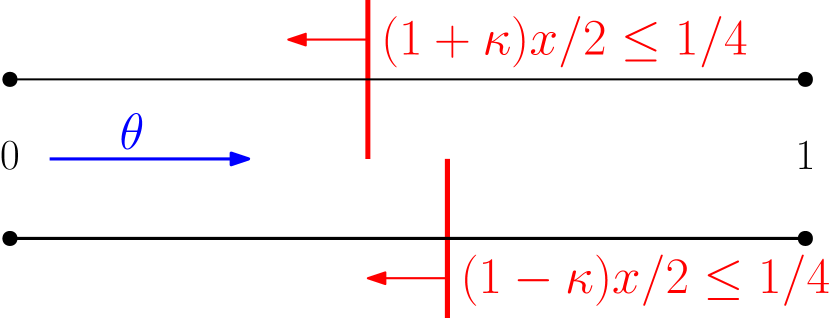
Figure 1: An obstruction to logarithmic bounds in safe linear bandits.

The result is shown in §F.1. The obstruction underlying this is illustrated in Figure 1. We study the $1$D problem $\max x$ under the known constraints $0\leq x\leq 1,$ reward parameter $\theta=1,$ and the unknown constraint $ax\leq 1/4$. Consider the case $a\in\{\nicefrac{{(1\pm\kappa)}}{{2}}\}$ for some $\kappa\in(0,1/4)$. The sets of extreme points in these two cases are $\{0,1,\nicefrac{{1}}{{2(1\pm\kappa)}}\}$, with the last point being optimal. In either case, the point $0$ has gap from optimal efficacy $(2(1\pm\kappa))^{-1}\geq 2/5$. Further, the point $1$ violates the constraint by $\nicefrac{{(1\pm 2\kappa)}}{{4}}\geq\frac{1}{8},$ and so both of these instances are at least $1/8$-well-separated.

But observe that no matter the $x_{t}$s, our estimates of $a$ must spread over a set of scale at least $1/\sqrt{t},$ and so we cannot eliminate either option for $a$ if $t<\kappa^{-2}.$ Now if the truth were $a=\nicefrac{{(1-\kappa)}}{{2}},$ but we played conservatively (i.e., $x_{t}<\nicefrac{{2}}{{1-\kappa^{2}}}$), we would incur an inefficacy of $\geq 2\kappa$. Similarly, if the truth were $a=\nicefrac{{(1+\kappa)}}{{2}},$ aggressive play ($x_{t}>\nicefrac{{2}}{{1-\kappa^{2}}}$) would violate safety by $2\kappa$. Thus, at least one of $\mathscr{E}_{T}$ and $\mathscr{S}_{T}$ must be $\Omega(\kappa\cdot\min(T,\kappa^{-2})).$ The bound follows by choosing $\kappa=1/\sqrt{T}$.

We highlight that the above lower bound scales as $\sqrt{T}$ despite constant order separation in the instance. This stands in sharp contrast to existing minimax lower bounds for standard bandits (e.g. Shamir; 2015), which set $\Delta\sim T^{-\nicefrac{{1}}{{2}}}$ in order to show $\Omega(\sqrt{T})$ bounds. The barrier to logarithmic control in SLBs is more fundamental, and comes from an inability to refine the precise location of the optimal point, rather than because there are suboptimal points in the noiseless problem that have similar performance. In other words, the issue is one of precision rather than one of hardness in the underlying LP. Nevertheless, the polytopal structure does induce a discreteness in the action space, through index sets of constraints. The following sections show and exploit this weaker discreteness.

5 Structural Behaviour of DOSLB, and Noise-Scale Lower Bounds

We proceed to formally define both the basic index sets that let us capture the underlying discreteness of the play of DOSLB, as well as the gaps associated with these index sets. The latter lead to the key consequence that ‘suboptimal’ index sets cannot be played too often by DOSLB.

5.1 Basic Index Sets

As in §4, index sets capture sets of known and unknown constraints. In other words,

Definition 4.

An index set is an ordered pair of sets $(\mathfrak{U},\mathfrak{K})$ such that $\mathfrak{U}\subseteq[1:U],\mathfrak{K}\subseteq[1:K]$. An index set $I=(\mathfrak{U},\mathfrak{K})$ is called a basic index set (BIS) if $|\mathfrak{U}|+|\mathfrak{K}|=d$.

Each BIS induces extreme points that activate the constraints it captures, as defined below.

Definition 5.

The set of points that activate an index set $I=(\mathfrak{U},\mathfrak{K})$ is defined as

$$\mathcal{X}^{I}:=\{x\in\mathcal{S}:A(\mathfrak{U})x=\alpha(\mathfrak{U}),B(\mathfrak{K})x=\beta(\mathfrak{K})\}.$$

Notice that we demand that activating points are feasible, i.e., that they lie in $\mathcal{S}.$ The set $\mathcal{X}^{I}$ may be empty, or a singleton, or an affine segment. We shall find the following terminology useful.

Definition 6.

A BIS $I$ is called $(\mathrm{(i)})$ feasible if $\mathcal{X}^{I}\neq\emptyset$ and infeasible otherwise; $(\mathrm{(ii)})$ suboptimal if $x^{*}\not\in\mathcal{X}^{I}$ and optimal otherwise; $(\mathrm{(iii)})$ full rank if the vectors $\{a^{i}\}_{i\in\mathfrak{U}}\cup\{b^{j}\}_{j\in\mathfrak{K}}$ span $\mathbb{R}^{d}$.

In the course of the bandit game, instead of the true constraint matrix $A$, we must work with noisy estimates of it, the $\tilde{A}$s. We extend the notion of BIS activation to handle this fuzziness in constraints.

Definition 7.

The set of points that noisily activates an index set $I=(\mathfrak{U},\mathfrak{K})$ at time $t$ is

$$\widetilde{\mathcal{X}}_{t}^{I}:=\{x\in\widetilde{\mathcal{S}}_{t}:\exists\tilde{A}\in\boldsymbol{\mathcal{{C}}}_{t},\tilde{A}(\mathfrak{U})x=\alpha(\mathfrak{U}),B(\mathfrak{K})x=\beta(\mathfrak{K}),\tilde{A}x\leq\alpha,Bx\leq\beta\}.$$

Note that $\widetilde{\mathcal{X}}_{t}^{I}\subset\widetilde{\mathcal{S}}_{t}$. The main structural result is the following observation.

Proposition 8.

The actions of DOSLB must noisily activate at least one BIS, i.e. $\forall t,\exists I_{t}:x_{t}\in\widetilde{\mathcal{X}}_{t}^{I_{t}}$.

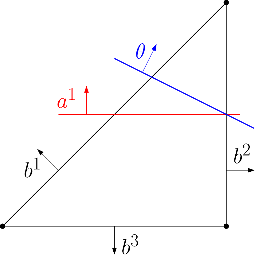
Figure 2: Illustration of Example 9. The black lines represent the known constraints, the red line is the unknown constraint, and the blue line is the locus of optimality.

If $x_{t}$ noisily activates the BIS $I$ at time $t$, we shall say that $I$ is played at time $t$. Note that more than one BIS may be played at a time (since $x_{t}$ can lie in the intersection of many $\widetilde{\mathcal{X}}_{t}^{I}$s).

Example 9.

To illustrate these definitions, consider the LP

$$\max x_{1}+2x_{2}:\underbrace{x_{2}\leq 1/2}_{\textrm{unknown}},\,\,\,\,\underbrace{x_{1}\geq x_{2},x_{1}\leq 1,x_{2}\geq 0}_{\textrm{known}}.$$

Foregoing normalisation for clarity, we have $U=1,K=3$ and the parameters $\theta=(1,2),a^{1}=(0,1),b^{1}=(-1,1),b^{2}=(1,0),b^{3}=(0,-1),\alpha=(0.5),\beta=(0,1,0)$. There are $\binom{1+3}{2}=6$ index sets,

$$I_{1}=(\{1\},\{1\}),I_{2}=(\{1\},\{2\}),I_{3}=(\{1\},\{3\}),$$

$$I_{4}=(\emptyset,\{1,2\}),I_{5}=(\emptyset,\{1,3\}),I_{6}=(\emptyset,\{2,3\}).$$

Of these, $I_{2}$ is optimal, and the rest suboptimal, with $x^{*}=(1,\nicefrac{{1}}{{2}}).$ Further, $I_{3}$ is rank-deficient while the rest are full-rank. Finally, $I_{3}$ and $I_{4}$ are infeasible, while the rest are feasible.

Also note that in the above example, the set $\mathcal{E}$ from §4 comprises of all the intersections of pairs of the constraints boundaries (i.e., points that lie on two black lines, or one black and the red line).

5.2 Gaps of Suboptimal BISs

We argue that if DOSLB noisily activates a suboptimal BIS at $t$, then the noise scale $\rho_{t}(x_{t};\delta)$ must be large. To show this, we develop two gaps for suboptimal BISs: the feasibility gap and the efficacy gap, which respectively exploit the permissibility and optimism of $x_{t}$. Our results will lower bound $\rho_{t}$ by the larger of these gaps when suboptimal BISs are played. The overall constructions are essentially via a reduction to linear programming sensitivity analysis, but with an additional complication thrown due to the fact that we need to handle general perturbations in the constraint values, rather than only studying the local behaviour of the optimal value under small perturbations. This is necessary: since we do not know the constraints in $A$ or $\theta$, perturbations in this matrix (as represented by $\tilde{A}$) may, and indeed do, cause the optimal $x^{*}$ to appear suboptimal.

The basic information we exploit is the following localisation of $x_{t}$, proved in §D.1.

Lemma 10.

Suppose the confidence sets are consistent, and that the action of DOSLB at time $t$, $x_{t},$ noisily activates the BIS $I=(\mathfrak{U},\mathfrak{K})$. Then the following relations hold true.

$$Ax_{t} \leq\alpha+\rho_{t}\mathbf{1}, Bx\leq\beta$$ (4)

$$A(\mathfrak{U})x_{t} \geq\alpha(\mathfrak{U})-\rho_{t}\mathbf{1},\qquad B(\mathfrak{K})x_{t}=\beta(\mathfrak{K}),$$ (5)

$$\left\langle\theta,x_{t}\right\rangle \geq\left\langle\theta,x^{*}\right\rangle-\rho_{t}.$$ (6)

This result follows as a straightforward application of Lemma 2, along with the definition of noisy activation, and the optimism and permissibility of $x_{t}$.

5.2.1 Intuitive Illustration of Gaps.

Let us first expose key components of the problem that allows doubly-optimistic plays to effectively control the play of suboptimal BISs through the specific case of a feasible, full-rank, and suboptimal BIS, using $I_{1}=(\{1\},\{1\})$ in Example 9. Due to the full-rank, the constraints of $I$ are activated by a unique point, i.e., $\exists x^{I}:\mathcal{X}^{I}=\{x^{I}\}.$ Since $I$ is suboptimal, $\xi(I):=\left\langle\theta,x^{*}-x^{I}\right\rangle>0.$ In our example, $x^{I_{1}}=(\nicefrac{{1}}{{2}},\nicefrac{{1}}{{2}})$, and $\xi(I_{1})=\nicefrac{{1}}{{2}}$.

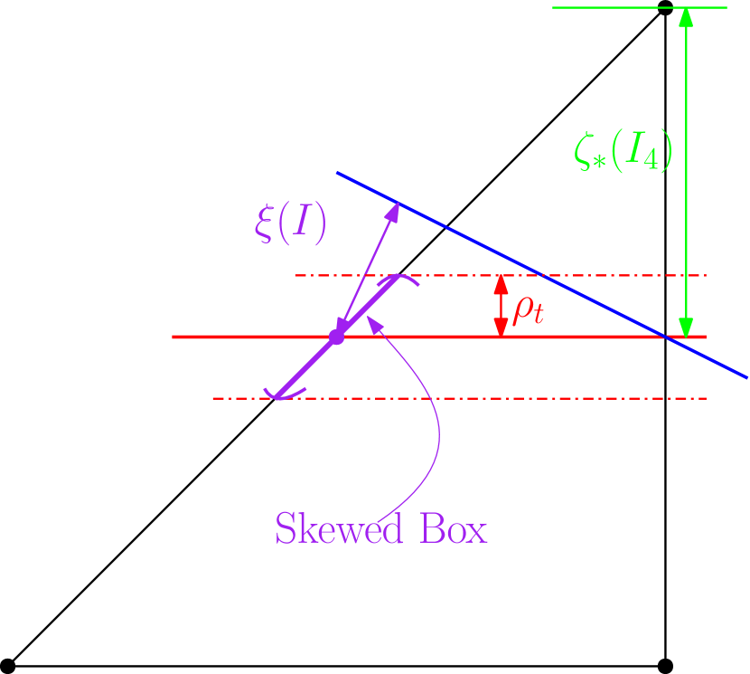
Figure 3: Illustration of gaps in Example 9. A $\rho_{t}$ perturbation in the unknown constraints is shown in red. $x^{I_{1}}$ is the purple dot, and the skewed box for $I_{1}$ under perturbations is shown in purple, along with $\xi(I_{1})$. The $\mathfrak{s}(I_{1})$ is the inner product of the direction in which the purple box varies, and $\theta$. For $I_{4},$ the feasibility separation $\zeta_{*}(I)$ is illustrated geometrically in green.

Efficacy Gap. Now, under noisy activation of $I$, the point $x_{t}$ may depart from $x^{I}$, but it cannot go too far. Indeed, by Lemma 10, $x_{t}$ must lie in a (skewed) $\ell_{\infty}$ box close to $x^{I},$ of ‘radius’ $\rho_{t}$. For $I_{1},$ this box is $\{x:x_{1}=x_{2},x_{2}\in\nicefrac{{1}}{{2}}\pm\rho_{t}\}.$

But this constrains how large $\left\langle\theta,x_{t}\right\rangle$ can be. Indeed, there exists a constant $\mathfrak{s}(I)$, such that moving in a unit box of this type can only increase $\left\langle\theta,x\right\rangle$ by at most $\mathfrak{s}(I)$—in effect, $\mathfrak{s}(I)$ is a measure of how well the geometry of this box aligns with $\theta$. This implies that $\left\langle\theta,x_{t}\right\rangle\leq\left\langle\theta,x^{I}\right\rangle+\rho_{t}\mathfrak{s}(I)$. For $I_{1},\mathfrak{s}(I)$ is the inner product between $(1,1)$ and $\theta,$ namely $\mathfrak{s}(I_{1})=3.$

Since $\left\langle\theta,x^{I}-x^{*}\right\rangle=-\xi(I)$, the above shows a tension with (6). Putting these together yields $\rho_{t}\geq\eta_{*}(I):=\xi(I)/(1+\mathfrak{s}(I)),$ a nontrivial constant lower bound on $\rho_{t}$. Such quantities are called the efficacy gap of $I$. For Example 9, $\eta_{*}(I_{1})=\nicefrac{{1}}{{8}}.$

Safety Gap. Of course, it is also possible that $x_{t}$ noisily activates an infeasible BIS, such as $I_{4}=(\emptyset,\{1,2\})$ in Example 9. In this case, a conflict arises between (4) and (5): when $\rho_{t}$ is small, any point meeting (4) is close to the safe set, but points meeting (5) are far from safety when $I$ is infeasible. In Example 9, (5) is only met by $(1,1)$ for $I_{4}$, but points meeting (4) must lie below $x_{2}=\nicefrac{{1}}{{2}}+\rho_{t}$. This means that there exists a minimal perturbation, $\zeta_{*}(I)$ such that if an infeasible BIS is noisily activated, then $\rho_{t}\geq\zeta_{*}(I).$ We call this the safety gap of $I$. In Example 9, $\zeta_{*}(I_{4})=\nicefrac{{1}}{{2}}.$

These two illustrations capture the two basic tensions in selecting suboptimal BISs. If the BIS is infeasible, then activating it requires that $\rho_{t}$ is at least larger than its safety gap, and if it is feasible but suboptimal, then activating the BIS requires that $\rho_{t}$ exceeds its efficacy gap. Below, we give a unified treatment of the above aspects by studying the behaviour of a parametrised LP with feasible set determined by (4) and (5), but with $\rho_{t}$ replaced by a parameter $\zeta$. The $\zeta_{*}(I)$ resolves to a feasibility condition for this parametrised LP, $\xi(I)$ is the minimal finite value attained by such programs, and $\mathfrak{s}(I)$ measures the sensitivity of the program with respect to $\zeta$.

5.2.2 Formal Definitions of the Gaps of Suboptimal BISs

We proceed with formalising the above discussion. Throughout, $I=(\mathfrak{U},\mathfrak{K})$ is a BIS.

Definition 11.

For a BIS $I$ and $\zeta\geq 0,$ the activation polytope of scale $\zeta$ induced by $I$ is defined as

$$\mathcal{T}(\zeta;I):=\{x:Ax\leq\alpha+\zeta\mathbf{1},A(\mathfrak{U})x\geq\alpha(\mathfrak{U})-\zeta\mathbf{1}(\mathfrak{U}),Bx\leq\beta,B(\mathfrak{K})x\geq\beta(\mathfrak{K})\}.$$

Further the optimistic LP at scale $\zeta$ induced by $I$ is defined as

$$P(\zeta;I):=\sup\{\left\langle\theta,x\right\rangle:x\in\mathcal{T}(\zeta;I)\}.$$

By Lemma 10, if $x_{t}$ noisily activates $I$, then $x_{t}\in\mathcal{T}(\rho_{t};I),$ and $\left\langle\theta,x_{t}\right\rangle\leq P(\rho_{t};I)$.

Feasibility Gap.

Notice that $P(\zeta;I)$ is right-continuous since its feasible set is a smoothly growing closed polytope. This means that for infeasible BISs, $P(0;I)=-\infty$, which motivates the following.

Definition 12.

We define the feasiblity gap of a BIS $I$ as

$$\zeta_{*}(I):=\inf\{\zeta\geq 0:P(\zeta;I)>-\infty\}.$$

Efficacy Gap.

As in §5.2.1, we need a notion of $\xi(I)$ and $\mathfrak{s}(I)$ to capture inefficacy of $I$.

Definition 13.

The efficacy separation of $I$ is defined as $\xi(I):=\left\langle\theta,x^{*}\right\rangle-P(\zeta_{*}(I);I)$. We further define the spread of $I$ as

$$\mathfrak{s}(I):=\inf\{C:\forall\zeta\geq\zeta_{*}(I),P(\zeta;I)\leq P(\zeta_{*}(I);I)+C(\zeta-\zeta_{*}(I))\}.$$

Notice that $\mathfrak{s}(I)$ is a measure of the sensitivity of $P(\zeta;I)$ with respect to its constraint levels (in other words, it is essentially a derivative). With these in hand, we can define the efficacy gap as below.

Definition 14.

The efficacy gap of a BIS $I$ is defined as

$$\eta_{*}(I):=\frac{\xi(I)}{1+\mathfrak{s}(I)}+\frac{\zeta_{*}(I)\mathfrak{s}(I)}{1+\mathfrak{s}(I)}.$$

$\eta_{*}$ is well-defined for infeasible BISs as well, and dominates $\zeta_{*}(I)$ iff $\xi(I)>\zeta_{*}(I)$.

Non-Triviality of Gaps.

Finally, we argue that the gaps we defined above are effective, i.e., that for any suboptimal BIS, at least one of these is non-zero. This is argued in §D.2 via a dual analysis.

Proposition 15.

For any suboptimal BIS $I$, $\mathfrak{s}(I)<\infty,$ and, a fortiori, $\max(\zeta_{*}(I),\eta_{*}(I))>0$.

5.3 Gap of the Problem, and Controlling the Play of Suboptimal BISs

We proceed to exploit the gaps of §5.2.1 to argue that suboptimal BISs cannot be played too often.

A Noise-Scale Lower Bound.

The following key result is shown in §D.2 using the ideas of §5.2.1.

Lemma 16.

If at time $t,$ the confidence sets are consistent and the action of DOSLB noisily activates the suboptimal BIS $I$, then $\rho_{t}\geq\max(\zeta_{*}(I),\eta_{*}(I)).$

Gap of an SLB Instance.

With the above in hand, the following definition is natural.

Definition 17.

The gap of an SLB instance is $\Xi:=\min\{\max(\zeta_{*}(I),\eta_{*}(I)):I\textrm{ is a suboptimal BIS}\}.$

Suboptimal BISs are rarely played.

We finally state the main result of this section, shown in §D.3.

Theorem 18.

Let $\{x_{t}\}$ denote the actions of DOSLB($\delta$) on a safe linear bandit problem. Then, with probability at least $1-\delta,$ if at any time $t,x_{t}$ noisily activates a suboptimal BIS, then $\rho_{t}>\Xi$. Further, the total number of times suboptimal BISs are played is bounded as

$$\sum_{t}\mathds{1}\{\exists\textrm{suboptimal BIS }I:x_{t}\in\widetilde{\mathcal{X}}_{t}^{I}\}=O\left(\frac{d^{2}\log^{2}T+d\log(T)\log(U/\delta)}{\Xi^{2}}\right).$$

This result implies that the preponderance of the time, DOSLB plays actions such that the noisy constraints they activate are precisely those that $x^{*}$ saturates. In other words, while the method may not be able to locate $x^{*}$ itself with precision better than $O(1/\sqrt{t}),$ it can identify the binding constraints, and, most of the time, the actions of DOSLB focus on activating these constraints.

6 Controlling Efficacy Regret and Total Safety Violation

We now come to the main results of the paper. The previous section tells us that suboptimal BISs cannot be played too often, effectively controlling a ‘dual’ type of regret. We proceed to translate these results into bounds on the ‘primal’ quantities $\mathscr{E}_{T}$ and $\mathscr{S}_{T}$. This requires us to account for the times when only optimal BISs ($I$ such that $x^{*}\in I$) are played. We can control the behaviour of such times under the following weak nondegeneracy condition at the optimum.

Assumption 19.

Every optimal BIS (i.e., $I:x^{*}\in\mathcal{X}^{I}$) is full-rank. Further, $\forall i,$ the noise $w_{t}^{i}$ is generic in the sense that the probability that $w_{t}^{i}$ lies in any subspace of less than $d$ dimensions is zero.

The assumption above leaves a lot of room for degeneracy, even at $x^{*}$, since any number of constraints can pass through it but no other point in $\mathcal{S}$. Of course, such non-degeneracy conditions are common in linear programming, and can in principle be addressed simply by perturbing the constraint matrix. Similarly, the noise genericity condition is standard (and can be met, e.g., by adding an arbitrarily small independent noise to the feedback). The main utility of this assumption is the following result, the first part of which is argued in §E.1 via a careful analysis of the optimistic selection rule (3) that characterises the structure of the noisy $\tilde{A}$ that the algorithm (implicitly) chooses when picking $x_{t}$.

Lemma 20.

Under assumption 19, if the confidence sets are consistent, $t\geq d+1,$ and the action $x_{t}$ of DOSLB($\delta$) is that $x_{t}$ only noisily activates the optimal BIS, then $\left\langle\theta,x_{t}\right\rangle\geq\left\langle\theta,x^{*}\right\rangle$. Further, for any $\varepsilon>0,$ if $\rho_{t}(x_{t})<\varepsilon,$ then for every $i$, $\left\langle a^{i},x_{t}\right\rangle\leq\alpha^{i}+\varepsilon.$

In other words, when the optimal BISs are played, then the action $x_{t}$ cannot be ineffective, and further cannot be too unsafe too many times. Notice that $\varepsilon$ is not delivered to the algorithm as a parameter, but instead the result above holds simultaneously for every $\varepsilon>0.$ This flexibility in $\varepsilon$ allows us to analyse the efficacy and safety properties of the play of DOSLB if we allow an arbitrary finite precision slack in the constraint levels. Concretely, let

$$\mathscr{S}^{\varepsilon}_{T}:=\sum\max_{i}(\left\langle a^{i},x_{t}\right\rangle-\alpha^{i}-\varepsilon)_{+}$$

denote the $\varepsilon$-precision safety violation. Coupling Lemma 20 and Theorem 18 yields the following.

Theorem 21.

Under assumption 19, $\forall\varepsilon,\delta>0,$ w.p. $\geq 1-\delta,$ the actions of DOSLB($\delta$) satisfy

$$\mathscr{E}_{T}=O\left(\frac{d^{2}\log^{2}(T)+d\log(T)\log(U/\delta)}{\Xi}\right)\ \ \text{and}\ \ \mathscr{S}_{T}^{\varepsilon}=O\left(\frac{d^{2}\log^{2}(T)+d\log(T)\log(U/\delta)}{\min(\Xi,\varepsilon)}\right).$$

A simulation study validating the above is presented in §7. Let us consider the behaviour represented above more closely.

Safety Properties.

The $\varepsilon$-precision safety violation $\mathscr{S}_{T}^{\varepsilon}$ is sublinear if and only if in most rounds, the actions of the algorithm are within $\varepsilon$ of the feasible set $\mathcal{S}$ in a stringent $\ell_{\infty}$ sense. Thus, $\mathscr{S}_{T}^{\varepsilon}$ captures the amount of violations up to an $\varepsilon$-precision tolerance in the constraint levels $\alpha^{i}.$ This metric is of strong relevance in the scenarios we discussed in §1, e.g., in drug trials, setting $\varepsilon$ to a fraction of the $\alpha^{i}$s lets us conclude that the potential over-exposure of drugs is marginal, as captured both by the net excess violation, and by the number of patients exposed to high doses. Let us again stress that the above behaviour holds simultaneously for every $\varepsilon>0$, and the algorithm does not receive $\varepsilon$ as an input. This means that the result adapts to the precision requirements of any domain.

Finite Precision Constraint Parameters. Rather than treating the precision in the levels $\alpha^{i},$ it is also possible that the entries of the constraint parameters $a^{i}$ are themselves restricted to a finite precision grid. Such a scenario occurs in drug discovery settings, where various latent ‘coverage’ constraints—which indicate if the drug binds to some set of receptors—are enforced, and naturally take binary values (e.g. Radhakrishnan and Tidor; 2008). More broadly, this applies to settings modeled as integer programs (up to given scaling). In such scenarios, the finite precision in the unknown $A$ matrix induces, under a mild modification of DOSLB , that there exists some $\varepsilon(\pi)$, a function of the precision $\pi$, such that each time the method plays unsafely, it must be at least $\varepsilon(\pi)$-unsafe, and so control on $\mathscr{S}_{T}^{\varepsilon(\pi)/2}$ directly controls safety violations $\mathscr{S}_{T}$.

Efficacy Properties.

The gain in efficacy that accrues from this slack in the safety measure is represented by the logarithmic control on $\mathscr{E}_{T}$: observe that this is an exponential improvement over the $\sqrt{T}$ efficacy regret incurred by PO methods. This fact means that when a slight tolerance is available in the system (but performance is measured relative to the nominal design values of the constraints), acting optimistically in the face of uncertain safety gives large advantages in terms of the efficiency of the online operation relative to operating conservatively, making it an important consideration and design approach for practitioners.

Exact Violations.

The simultaneity of Theorem 21 in $\varepsilon$ also lets us derive control on $\mathscr{S}_{T}.$ Indeed, note that $\mathscr{S}_{T}\leq\mathscr{S}_{T}^{\varepsilon}+\varepsilon T$. Optimising over $\varepsilon$ in the bound of Theorem 21, as we do in§E.3.1 yields

Corollary 22.

Assuming 19, with high probability, the actions of DOSLB($\delta$) satisfy

$$\mathscr{E}_{T}=O(d^{2}\log^{2}T/\Xi),\quad\textrm{and}\quad\mathscr{S}_{T}=\widetilde{O}(d\sqrt{T}).$$

Observe that this is optimal in light of Theorem 3. Thus, up to logarithmic terms, doubly-optimistic play in SLBs saturates the tradeoff inherent in this lower bound in favour of minimal efficacy regret.

Tightness of Dependence on $\Xi$.

Exploiting a subtle reduction of safe Multi-Armed Bandits problems to SLB problems, we show in §F.2 that the inverse dependence on $\Xi$ is necessary.

Theorem 23.

Fix a $c\in(0,1)$. For any $\Xi\leq\nicefrac{{1}}{{16}},$ and any method that ensures that in every SLB instance, $\max(\mathscr{E}_{T},\mathscr{S}_{T})=O(T^{1-c}),$ there exists an instance of the SLB problem with gap at least $\Xi,$ such that $\liminf\frac{\max(\mathbb{E}[\mathscr{E}_{T}],\mathbb{E}[\mathscr{S}_{T}]}{\log T}\geq\nicefrac{{c}}{{108}}\cdot\Xi^{-1}\log T.$

This result applies to DOSLB, since it achieves $\max(\mathscr{E}_{T},\mathscr{S}_{T})=\widetilde{O}(\sqrt{T})$ in general (§E.3.2).

Finite Action Spaces.

A common condition in linear bandits is to assume that the learner is provided a finite set of actions $\mathcal{A},$ and must ensure $x_{t}\in\mathcal{A}$ (e.g. Abbasi-Yadkori et al.; 2011). This scenario considerably simplifies our analysis, since resolving the optimal point is no longer a concern, and so the entire analysis can be performed in the primal space. Indeed, let us modify DOSLB so that its makes its optimistic choice from $\widetilde{\mathcal{S}}_{t}\cap\mathcal{A}$, and define the finite-arm efficacy gap of $x\in\mathcal{A}$ as $\Delta_{x}:=\left\langle\theta,x^{*}-x\right\rangle_{+}$ and the finite-action safety gap of $x\in\mathcal{A}$ as $\Sigma_{x}:=\max_{i}(\left\langle a^{i},x\right\rangle-\alpha^{i})_{+},$ and the gap of the problem as $\Gamma:=\min_{x\in\mathcal{A}}\max(\Delta_{x},\Sigma_{x}).$

Proposition 24.

With probability at least $1-\delta,$ the modified finite-action DOSLB achieves the following bounds in the finite-armed SLB setting: $\max(\mathscr{E}_{T},\mathscr{S}_{T})=O(d^{2}\log^{2}T/\Gamma).$

Notice that we do not need a precision relaxation in $\mathscr{S}_{T}$ above, because the precision issues arising from having to locate the optimal action are not present.

7 Simulations

We verify the theoretical study above with simulations over Example 9, and study the relative performance of DOSLB and the optimistic-pessimistic method Safe-LTS Moradipari et al. (2021). These implementations are based on the following relaxation of Algorithm 1.

7.1 Computationally Feasible Relaxation

A well-known barrier to implementing Algorithm 1 is that even if all constraints were known, the program (3) is non-convex (Dani et al.; 2008). In our case, this is further complicated by the fact that the set $\widetilde{\mathcal{S}}_{t}$ needs to be determined, which too is computationally subtle.

We approach these issues by constructing box confidence sets. We consider two relaxations to this, the $L_{\infty}$ box and the $L_{1}$ box, as follows:

$$\mathcal{C}_{t,\infty}^{i}:=\{\tilde{a}:\|(\tilde{a}-\hat{a}^{i})V_{t}^{1/2}\|_{\infty}\leq\sqrt{\beta_{t}}\},$$

$$\mathcal{C}_{t,1}^{i}:=\{\tilde{a}:\|(\tilde{a}-\hat{a}^{i})V_{t}^{1/2}\|_{1}\leq\sqrt{d\beta_{t}}\},$$

such that $\mathcal{C}_{t}^{i}\subset\mathcal{C}_{t,\infty}^{i}$ and $\mathcal{C}_{t}^{i}\subset\mathcal{C}_{t,1}^{i}$, since $L_{2}$ ball with radius $r$ is contained in $L_{1}$ ball with radius $r$ and $L_{\infty}$ ball with radius $\sqrt{d}r$. Take any $\tilde{a}\in\mathcal{C}_{t,\infty}^{i}$, $\|(\tilde{a}-\hat{a}^{i})V_{t-1}^{1/2}\|_{\infty}\leq\sqrt{\beta_{t-1}}\implies\|(\tilde{a}-\hat{a}^{i})V_{t-1}^{1/2}\|_{2}\leq\sqrt{d\beta_{t-1}}$, and the same holds for the $L_{1}$ relaxation as well. Thus replacing $\mathcal{C}_{t}^{i}$ by $\mathcal{C}_{t,\infty}^{i}$ or $\mathcal{C}_{t,1}^{i}$, the only change in analysis will be from $\rho_{t}$ to $\overline{\rho}_{t}=\sqrt{d}\rho_{t}$. Hence running DOSLB with these worsens regret bounds by at most $O(\sqrt{d})$ (and the relaxed regret bound by at most $O(d)$).

The principal advantage of using $\mathcal{C}_{t,\infty}$ lies in the fact that the box-confidence sets are polytopes. Due to this, the values of $\tilde{\theta}\in\mathcal{C}_{t-1,\infty}^{0}$ and $\tilde{a}^{i}\in\mathcal{C}_{t-1,\infty}^{i}$ that are active for the optimistic action $x_{t}$ must lie at the extreme points of these sets. Since each set has only $2d$ extreme points, this allows us to determine $x_{t}$ by solving $(2d)^{U+1}$ convex programs, which is computationally feasible so long as $U$ is small. Of course, this complexity remains painfully slow as $U$ grows. Finding versions of the doubly-optimistic strategy that are computationally practical for a large number of unknown constraints remains an interesting open problem.

To investigate the choice between these two relaxations, we simulated DOSLB with each of these on the instance of Example 9. We find that while both show very strong efficacy and acceptable safety violations, the $L_{1}$ relaxation appears to be more aggressive, and thus has weaker safety properties. See §G for the observations.

7.2 Results

We implement DOSLB on with the $L_{\infty}$ relaxation above on the instance of Example 9 over the horizon $T=10^{4},$ and with the parameters $\lambda=2,\delta=1/(4T)=2.5\times 10^{-5}.$ The noise in observations is independent and Gaussian, with variance $0.1$. Notice that for this instance, $\Xi=\nicefrac{{1}}{{8}}$.

7.2.1 The behaviour of DOSLB

Our key observations regarding the behaviour of DOSLB are as follows.

DOSLB is very effective, and has well-controlled violations.

Figure 4 shows the efficacy regret $\mathscr{E}_{t}$ and both the arbitrary precision safety violations $\mathscr{S}_{t}$ and the finite precision safety violations $\mathscr{S}_{t}^{\varepsilon}$ for the value $\varepsilon=0.05=2\Xi/5$. The observations strongly validate our main claims of strong efficacy regret control, and well-behaved growth of safety violations. Indeed, observe that the efficacy regret is essentially zero over most of the runs (with rare runs rising to $\mathscr{E}_{10^{4}}\approx 100$). This property arises since DOSLB very rarely plays suboptimal BISs (see the following discussion and Figure 5), and when it plays the optimal BIS, it plays a ‘over-efficient’ but unsafe point. Further, the extent of the lack of safety of the actions chosen by DOSLB is well-controlled, as seen in the behaviour of $\mathscr{S}_{T}$. The finite precision regret shows even stronger control, with growth essentially halted at $t\approx 5000,$ validating the analysis underlying Theorem 21.

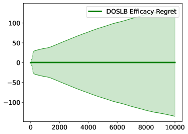
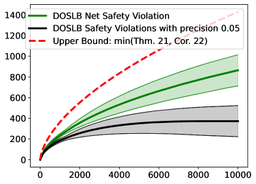
Figure 4: Efficacy Regret and Safety Violation of DOSLB . We plot averages and one standard deviation confidence regions over 30 runs for $\mathscr{E}_{T}$ (left) and both $\mathscr{S}_{t}$ and $\mathscr{S}_{t}^{0.05}$ (right). We also plot the upper bounds we show in the latter to contextualise the observations. Observe that the efficacy regret is marginal: the mean is essentially $0,$ and the variance limited. Further, observe that the growth of the net safety violation $\mathscr{S}_{t}$ is well-controlled, and lies far below the bounds of §6. Further, the finite precision violations show a strong flattening, as is expected from Theorem 21.

DOSLB rarely activates suboptimal index sets.

In Figure 5, we plot the number of times that DOSLB noisily activates a suboptimal BIS, i.e., any index set other than $I_{2}=(\{1\},\{2\})$. The main observation is that this occurs very rarely: indeed, over the horizon of $10^{4}$, most runs do not activate suboptimal BISs more than 100 times. This is far below the upper bound of Theorem 18.

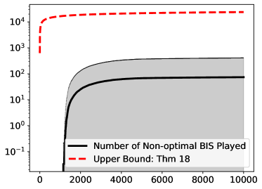
Figure 5: Number of times a suboptimal BIS is noisily activated by DOSLB in the instance of Example 9. Means over and one standard deviation over 30 runs are reported, and the vertical scale is logarithmic. Observe that the method activates such index sets very rarely, typically far less than $1\%$ of the times. Also observe that the growth is essentially flat.

7.2.2 DOSLB Compares Favourably with Pessimistic-Optimistic Methods.

To contextualise our method, we also implement the PO-method safe-LTS due to Moradipari et al. (2021) in the instance of Example 9. As previously discussed, safe-LTS constructs a pessimistic set of permissible points, $\Pi_{t}$, such that with high probability all points in $\Pi_{t}$ must be safe. The method then selects actions optimistically, in this case by exploiting Thompson sampling. The safe point provided to safe-LTS is $x^{\mathsf{s}}=(0,0),$ which has the separation $M^{\mathsf{s}}=\nicefrac{{1}}{{2}}.$

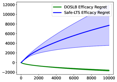
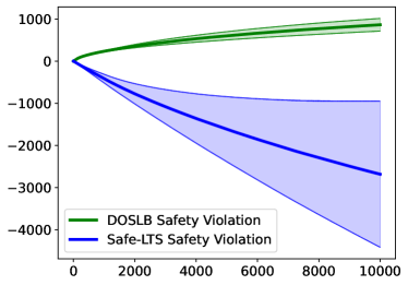
Figure 6: Comparing the behaviour of DOSLB and safe-LTS on the instance of Example 9. The left plot shows the raw efficacy regret, while the right plot is the raw safety violations of the two methods, and each reports means and one-standard deviation confidence regions over 30 runs.. Observe that the efficacy performance of safe-LTS is extremely poor, indicating that the algorithm is far from the boundary of the safe set $\mathcal{S}$ for most of its runs. In contrast, the violation properties of DOSLB are well-controlled, and almost four times smaller than the efficacy regret of safe-LTS.

Figure 6 compares the behaviour of the raw efficacy regret $\sum\left\langle\theta,x^{*}-x_{t}\right\rangle$ (left) and the raw safety violation $\sum\max_{i}(\left\langle a^{i},x_{t}\right\rangle-\alpha^{i})$ (right) of Safe-LTS and DOSLB (since the efficacy regret of DOSLB , and the safety-violations of safe-LTS are both essentially $0$, the raw behaviour elucidates more insight). As expected, safe-LTS suffers from $0$ safety regret, since it plays in a pessimistic set. However, this is accompanied by a large efficacy regret, with the mean of over $7000$ at the horizon $T=10^{4}$. This arises due to the extreme conservatism of this method, which is evident from its safety violation property: the method has a strong negative (and decreasing still) violation, indicating that it continues to play deep in the interior of the domain for large $T$. Indeed, since over the domain, $\left\langle a,x\right\rangle-\alpha\in[-0.5,0.5],$ and since the violation at $T=10^{4}$ is roughly $-3000,$ this indicates that with a nontrivial probability, the method remains at least $0.25$-separated from the boundary of the safe set.

In comparison, observe that the raw efficacy regret of DOSLB is negative, but not nearly as far as the violations of safe-LTS. This indicates that the method is shrinking towards the boundary of the safe set at a much better rate. Of course, this property is similarly illustrated by the violation behaviour: this nearly four times smaller than the efficacy regret of safe-LTS, and concentrates strongly to $\approx 800$ at $T=10^{4}$.

8 Discussion

The Safe Linear Bandit probem is inherently challenging due to the roundwise enforcement of constraints. Taking a pragmatic view to justify the same, the above study focuses on soft constraint enforcement using aggressive ‘doubly-optimistic’ methods, partly in an effort to improve upon the poor efficacy and strong assumptions required for hard enforcement of the same. To this end, we first identified a critical and fundamental source of hardness in SLBs, the inability to resolve optimal points to arbitrary precision and thus to meet constraints to arbitrary precision with subpolynomial violations and regret.

Motivated by the soft view espoused above, we then proposed a natural confidence-bound based doubly optimistic method, and gave a refined characterisation of its behaviour. In particular, we showed that the optimistic structure has favourable behaviour in a dual sense, in that most of the time such play activates optimal index sets, and, under a mild structural assumption, controlled the regret to polylogarithmic scale in terms of the horizon $T$. We further characterised the safety violation in the course of such play, showing that in general it is bounded as $\tilde{O}(\sqrt{T}),$ and up to an arbitrary finite precision, it instead is bounded at polylogarithmic scales in $T$. Our simulations both bear out this analysis, and further illustrate that the violation behaviour of our doubly-optimistic method is considerably better behaved than the inefficacy of prior PO methods. These represent extremely large efficacy gains, at a relatively mild safety violation cost, making the use of doubly-optimistic methods quite relevant to practical study of constrained linear optimisation under stochastic bandit feedback.

A number of interesting directions remain open, both specifically for safe linear bandits, and for constrained learning in general. We discuss a few of these below.

Broadly speaking, the doubly-optimistic principle of course extends to general stochastic online learning problems with latent constraints. It is natural to ask if such an approach is similarly powerful in richer models, for instance contextual bandits, or MDPs (over the trajectory, rather than episodically), and whether a similarly refined analysis can be performed in such settings. Such questions are of course critical to the applicability of this approach, since most practical problems are far richer than a simple bandit structure.

On the technical front, there are a plethora of question left unanswered, and we highlight three of these. Firstly, we ask if Assumption 19 can be relaxed. Indeed, while this nondegeneracy condition is quite weak, and would not in general preclude the use of this approach, it is unclear if such a condition is necessary. For instance, is it always the case that at least one of the noisy BISs that $x_{t}$ saturates is optimal? What if the noise scale is small? These questions demand a closer understanding of the optimistic selection rule, and their resolution is bound to be interesting. Secondly, we mention that while the method can, with a small loss in regret, be implemented, the per-round complexity of our implementation is $d^{U+1},$ making it impractical when there are a large number of unknown constraints. Alternative doubly-optimistic algorithms, or faster approximations to DOSLB, are thus a crucial and interesting question, theoretically, as well as practically due to the large gains of optimistic play. Along these lines, one natural question is whether a Bayesian construction of a permissible set is a viable attack. Such constructions must be subtle—even in multi-armed bandits, a naïve generalisation of Thompson sampling is ineffective (Chen et al.; 2022). Thirdly, and more broadly, is the interesting question of how one mix the behaviours of the PO and DO methods. For instance, is it possible to start out playing doubly optimistically, and quickly gain a lot of information at some safety cost, and then ameliorate this cost by a persistent pessimistic play?

Finally we mention potential implications of our study on the pure exploration questions. Observe that since the above method concentrates strongly on activating only optimal BISs, in a pure exploration sense it should similarly be possible to identify optimal BISs. In other words, in an applied setting, while we may not be able to exactly nail down the constraint itself, we should be able to easily tell that it is binding at the optimum (e.g., we may not be able to model exactly what increases customer friction, but we can certainly tell that this limits how aggressively we can test proposals). Such information can be quite valuable, both for directing strategy and for focusing research directions. This motivates the question of what the sample complexity of such identification is in a pure exploration setting, which may be an interesting weakening of the solution concept that may be exploited to go beyond the finite action set assumptions made in the current literature on identifying the best feasible arms.

Appendix A A More Detailed Look at PO methods.

Structurally the PO based methods all demand the knowledge of a point $x^{\mathsf{s}}$ and a constant $M^{\mathsf{s}}>0$ such that it is known a priori that the point $x^{\mathsf{s}}$ satisfies $\max_{i}\left\langle a^{i},x^{\mathsf{s}}\right\rangle-\alpha^{i}\leq-M^{\mathsf{s}},$ i.e., that $x^{\mathsf{s}}$ is very safe. Notice that under the assumption that $\|x\|$ and $\|a^{i}\|$ are bounded, this yields a small ball $\mathcal{B}^{\mathsf{s}}$ around $x^{\mathsf{s}}$ of size scale $M^{\mathsf{s}}$ that must be safe (this is the way we stated this assumption in the main text). PO methods proceed by building, in each round $t$, a pessimistic set $\Pi_{t}$ such that with high probability, every $\Pi_{t}\subset\mathcal{S},$ i.e., every action in $\Pi_{t}$ must be safe. Notice that $\Pi_{t}$ is guaranteed to be nonempty since $\mathcal{B}^{\mathsf{s}}\subset\Pi_{t}$ - this is the main role of $\mathcal{B}^{s}$. Since $\Pi_{t}$ is an inner approximation to the true safe set, these methods are ‘pessimistic’ about the safety property of potential actions. PO methods then pick an action by maximising an optimistic reward index amongst actions in $\Pi_{t}$, i.e., by maximising $\max_{\tilde{\theta}\in\mathcal{C}_{t}^{0}}\langle\tilde{\theta},x\rangle$. For small $t$, this essentially amounts to a random scan over a (slightly enlarged neighbourhood of) $\mathcal{B}^{s}$. Therefore, it is natural that the scale $M^{\mathsf{s}}$ appears inversely in the regret bounds, the best of which are of the form $O((M^{\mathsf{s}})^{-1}\sqrt{T})$, since this limits the signal strength of the initial exploration. Both the requirement of knowing $(x^{\mathsf{s}},M^{\mathsf{s}})$, and the dependence of the bounds on $M^{\mathsf{s}}$ are siginificant disadvantages of these methods, although these requriements are necessary: to always be safe, we necessarily need to begin at a safe place, and should have some room to explore around it. Quantitatively, both the inverse dependence on $M^{\mathsf{s}}$ and the dependence on $\sqrt{T}$ are necessary even in well-separated instances (Pacchiano et al. [2021] show the former, and our Theorem 3 shows the latter).

In linear bandits, the PO approach was first considered by Amani et al. [2019], although they rely on a weaker phased explore-and-commit strategy (where the exploration is limited to the set $\mathcal{B}^{\mathsf{s}}$ above), and give weaker $\Omega(T^{2/3})$ bounds on $\mathscr{E}_{T}$ when considering a single constraint (i.e., $U=1$). Subsequently, Moradipari et al. [2021] refined this approach in two ways: the pure exploration phase is eliminated, and instead the algorithm, Safe-LTS, constructs the pessimistic safe set $\Pi_{t}$ as above, and uses Thompson sampling to select the action $x_{t}$. We caution the reader that this (single unknown constraint) scheme is analysed under the assumption that $\alpha^{1}>0,$ and it is assumed that the origin is safe. Thus $\alpha^{1}$ itself behaves as $M^{\mathsf{s}}$. The authors show (efficacy) regret bounds of $O(\sqrt{d^{3}T}/\alpha^{1}).$

Pacchiano et al. [2021] mix the PO view with lifting the action space to policies, i.e., distributions over $x_{t}$. Concretely, this work demands that at each time $t$, the algorithm produces a distribution $\pi_{t}$ such that $\mathbb{E}_{x\sim\pi_{t}}[\left\langle a^{1},x\right\rangle]\leq\alpha^{1}$, while the goal is to maximise the reward $\mathbb{E}_{x\sim\pi}[\left\langle\theta,x\right\rangle],$ and the optimal safe policy is called $\pi^{*}$. Actual points are selected, of course, by sampling from $\pi_{t}$, and noisy version of the corresponding inner products are given as feedback. The principal observation in light of the safety criterion is that while ostensibly round-wise, this study is in fact fundamentally enforcing only an aggregate constraint. This arises since the optimal policy $\pi^{*}$ is only required to be safe in expectation, and so may place non-trivial mass on unsafe points. Indeed, such behaviour has been demonstrated both theoretically and empirically in the case of multi-armed bandits Chen et al. [2022].

More recently, Bernasconi et al. [2022] study a linearised approach to tree-form sequential games, which comprise a special case of a finite state and action sequential decision making problem. The approach taken is again linearisation, and both soft and hard constraint satisfaction are studied, although the form the methods take are somewhat simplified because the potential extreme points, i.e. the set $\mathcal{E}$ from §4 is known a priori. We also note that this hard approach has been studied for exploration in the finite state-action MDP literature, where the demand is to learn a policy with high value while ensuring that each state visited in the trajectory is safe [e.g. Turchetta et al., 2016, Wachi and Sui, 2020].

Appendix B On the Assumptions, and Background on Online Linear Regression

We give an expanded discussion of the standard assumptiosn made in §2, and discuss a standard result from online linear regression controlling $\sum\|x_{t}\|_{V_{t-1}^{-1}}$ that is key to our analysis.

B.1 A closer look at the assumptions

The assumptions made in the main text are slightly simplified version of standard assumptions from the literature on linear bandits.

Boundedness. The boundedness assumption has two parts: firstly that the underlying parameters are bounded, i.e., $\|\theta\|,\|a^{i}\|\leq 1$ and secondly we assume that the domain is bounded, i.e., $\|x\|\leq 1$ for all $x\in\mathcal{X}=\{Bx\leq\beta\}$.

The bounded domain assumption is used chiefly to ensure that the underlying optimisation problem of interest has finite value. Quantitatively, this may be replaced with a generic bound $\|x\|\leq L$ instead without appreciably changing the study. The principal way this affects DOSLB is via the choice of the regulariser $\lambda$ - concretely, the validity of Lemma 1 requires that $\lambda\geq\max_{t}\|x_{t}\|^{2},$ which may be ensured by setting $\lambda\geq L^{2}$. Indeed, this fact underlies our choice of $\lambda=1$ in the main results. A second aspect that is affected by the quantity $L$ is that the upper bound of Lemma 25 would read $\log(1+TL^{2}/\lambda d)$ instead of $\log(1+T/\lambda d)$, which mildly affects some logarithmic terms in the regret bounds.

The assumption of bounded parameters is largely without loss of generality - indeed, if we had a bound $\|\theta\|,\max_{i}\|a^{i}\|\leq S$ instead, the only change required is that the confidence set radius $\omega_{t}$ would need to be set as

$$\sqrt{\omega_{t}(\delta;S)}=\sqrt{\omega_{t}(\delta;1)}+(S-1)\sqrt{\lambda},$$

i.e., only the additive $\sqrt{\lambda}$ term in $\sqrt{\omega_{t}}$ from the main text would need adjustment. We note that in general, the norm bounds on the various $a^{i}$ and $\theta$ need not agree, and it is in fact possible to adapt to their norms without prior knowledge of the same, by setting distinct $\omega_{t}^{i}$s for each $a^{i}$, and using the techniques of the recent work of Gales et al. [2022].

SubGaussianity. While the subGaussianity condition can also be relaxed (for instance, linear bandits with heavy tailed noise have been studied [Shao et al., 2018]), it yields significant technical convenience whilst remaining quite a generic setting. In the assumption, we concretely assume that the noise is conditionally $1$-subGaussian. This may be relaxed to conditionally $R$-subGaussian. This too can be handled with a small change in $\omega_{t}$ to

$$\sqrt{\omega_{t}(\delta;R)}=R\sqrt{\frac{1}{2}\log\left(\frac{(U+1)\det(V_{t})^{1/2}\det(\lambda I)^{-1/2}}{\delta}\right)}+\lambda^{1/2}.$$

This change is somewhat stronger than the corresponding change induced by altering $\|\theta\|$ and $\|a^{i}\|$, since the scaling is now applied to the first term of $\omega_{t},$ which grows with $t$ unlike the constant $\sqrt{\lambda}$ penalty.

Overall Confidence Radius with General Parameters. To sum up, under the generic conditions $\|x\|\leq L,\|\theta\|\leq S,\|a^{i}\|\leq S,$ and $R$-subGaussianity of $\{\gamma_{t}^{i}\}$, the entirety of our following analysis will go through, but with the blown up confidence radii

$$\sqrt{\omega_{t}(\delta;L,S,R)}=R\sqrt{\frac{1}{2}\log\left(\frac{(U+1)\det(V_{t})^{1/2}\det(\lambda I)^{-1/2}}{\delta}\right)}+S\lambda^{1/2},$$

and under the condition $\lambda\geq L$. This results in roughly an increase in the regret bounds of a factor of at most $\max(R,S),$ along with a potential increase in the logarithmic terms to $\log(1+TL^{2}/\delta)$ instead of $\log(1+T/\delta)$. For the remainder of our analysis, we shall stick to the default parameters $R=S=L=1$.

B.2 Quantitative Bounds from the Theory of Online Linear Regression

We conclude the preliminaries with the following generic statement, which holds due to a couple of applications of the matrix-determinant lemma. The result is standard - see the discussions of Abbasi-Yadkori et al. [2011, Lemma 11] for historical discussions.

Lemma 25.

Let $\{x_{t}\}$ be the actions of DOSLB. Suppose that for all $t$, $\|x_{t}\|\leq 1$, and let $\lambda\geq 1$. Then for any $T$,

$$\sum_{t=1}^{T}\|x_{t}\|_{V_{t-1}^{-1}}^{2}\leq\frac{3}{2}\log\left(\frac{\mathrm{det}(V_{T})}{\mathrm{det}(\lambda I)}\right)\leq\frac{3}{2}d\log\left(1+\frac{T}{\lambda d}\right).$$

Proof of Lemma 25.

First notice that since $V_{t}=V_{t-1}+x_{t}x_{t}^{\top},$ by the matrix-determinant lemma,

$$\det(V_{t})=\det(V_{t-1})\det(I+V_{t-1}^{-1/2}x_{t}x_{t}^{T}(V_{t-1}^{-1/2})^{\top}=\det(V_{t-1})(1+\|x_{t}\|_{V_{t-1}^{-1}}^{2}),$$

and induction yields

$$\det(V_{T})=\det(\lambda I)\prod(1+\|x_{t}\|_{V_{t-1}^{-1}}^{2}).$$

where we have used that $V_{0}=\lambda I.$

Now, notice that since $V_{t-1}\succ\lambda I$ for each $t$, it follows that $\|x_{t}\|_{V_{t-1}^{-1}}^{2}\leq\|x_{t}\|^{2}/\lambda\leq 1.$ But for $z\in[0,1],z\leq\frac{3}{2}\log(1+z),$ which implies that

$$\sum\|x_{t}\|_{V_{t-1}^{-1}}^{2}\leq\frac{3}{2}\sum\log(1+\|x_{t}\|_{V_{t-1}^{-1}}^{2})=\frac{3}{2}\log\frac{\det(V_{T})}{\det(\lambda I)}.$$

Finally, note that since $V_{T}$ is positive definite, by an application of the AM-GM inequality, ${\det(V_{T})}\leq(\mathrm{trace}(V_{T})/d)^{d}$, and further, $\mathrm{trace}(V_{T})=d\lambda+\sum_{t}\|x_{t}\|_{2}^{2}\leq d\lambda+T.$ Further observing that $\det(\lambda I)=\lambda^{d},$ we conclude that

$$\log\frac{\det(V_{T})}{\det(V)}\leq d\log\frac{(d\lambda+T)/d}{\lambda}=d\log\left(1+\frac{T}{d\lambda}\right).$$

∎

An immediate consequence of the above is the following pair of observations which we shall use frequently.

Lemma 26.

Let $\{x_{t}\}$ be the actions of DOSLB run with the parameters $\lambda,\delta$. For every $T>0,$

$$\sum_{t\leq T}\rho_{t}(x_{t};\delta)^{2} \leq 3d^{2}\log^{2}\left(1+\frac{T}{\lambda d}\right)+6d\log\left(1+\frac{T}{\lambda d}\right)\left(\log\frac{U+1}{\delta}+2\lambda\right),$$ (7)

$$\sum_{t\leq T}\rho_{t}(x_{t};\delta) \leq d\sqrt{3T}\log\left(1+\frac{\log T}{d\lambda}\right)+\sqrt{3dT\log\left(1+\frac{T}{\lambda d}\right)}\left(\sqrt{2\lambda}+\sqrt{\log\frac{U+1}{\delta}}\right).$$ (8)

These bounds supply the core bounds needed to convert the control we develop on $\rho_{t}$ in §5.3 and §6 into control on $\mathscr{E}_{T}$ and $\mathscr{S}_{T}$. Observe that the main terms in the above results do not show dependence on the failure probability parameter $\delta$.

Proof of Lemma 26.

Recall that $\rho_{t}(x_{t};\delta)=2\sqrt{\omega_{t}(\delta)}\cdot\|x_{t}\|_{V_{t-1}^{-1}}.$ Further observe that $\omega_{t}$ is an increasing function of $t$. Immediately by Lemma 25,

$$\sum\rho_{t}^{2}\leq 4\omega_{T}(\delta)\sum\|x_{t}\|_{V_{t-1}^{-1}}^{2}\leq 6d\omega_{T}(\delta)\log\left(1+\frac{T}{d\lambda}\right).$$

Further, once again applying Lemma 25, and noting that $(\sqrt{u}+\sqrt{v})^{2}\leq 2u+2v,$

$$\sqrt{\omega_{T}(\delta)} =\sqrt{\lambda}+\sqrt{\frac{1}{2}\log\frac{(U+1)}{\delta}+\frac{1}{4}\log\frac{\det(V_{T})}{\det(\lambda I)}}$$

$$\implies\omega_{T}(\delta) \leq 2\lambda+\log\frac{(U+1)}{\delta}+\frac{d}{2}\log\left(1+\frac{T}{\lambda d}\right).$$

Multiplying these two bounds controls $\sum\rho_{t}^{2}.$

Further, by the Cauchy-Schwarz inequality,

$$\sum_{t=1}^{T}\rho_{t}\leq\sqrt{T}\cdot\sqrt{\sum_{t=1}^{T}\rho_{t}^{2}}.$$

The bound (8) follows upon applying the bound on $\sum\rho_{t}^{2}$ above, and then using the trivial relation $\sqrt{u+v}\leq\sqrt{u}+\sqrt{v}$. ∎

Finally, let us argue that the quantity $\rho_{t}(x_{t};\delta)$ indeed controls the noise scale of the problem by showing Lemma 2.

Proof of Lemma 2.

Let us take the case of $\theta$. The bounds for the $a^{i}$s arise in exactly the same way. Under the assumption of consistency, $\theta\in\mathcal{C}_{t}^{0}$. Therefore

$$|\langle\tilde{\theta}-\theta,x\rangle|\leq|\langle\tilde{\theta}-\hat{\theta},x\rangle|+|\langle\theta-\hat{\theta},x\rangle|.$$

By exploiting the positive definiteness of $V_{t-1}$ and the Cauchy-Schwarz inequality, we can further observe that

$$|\langle\theta-\hat{\theta},x\rangle| =|\langle(\theta-\hat{\theta})V_{t-1}^{1/2},V_{t-1}^{-1/2}x\rangle|\leq\|\theta-\hat{\theta}\|_{V_{t-1}}\cdot\|x\|_{V_{t-1}^{-1}}.$$

Running the same calculation of $\tilde{\theta}$ and adding the bounds, we conclude that

$$|\langle\tilde{\theta}-\theta,x\rangle|\leq(\|\theta-\hat{\theta}\|_{V_{t-1}}+\|\tilde{\theta}-\hat{\theta}\|_{V_{t-1}})\|x\|_{V_{t-1}^{-1}}$$

But both $\theta,\tilde{\theta}\in\mathcal{C}_{t}^{0},$ which by definitions means that their $V_{t-1}$-norm distance from $\hat{\theta}$ is bounded by $\sqrt{\omega_{t-1}(\delta)}.$ The claim is immediate upon recalling that $\rho_{t}(x;\delta):=2\sqrt{\omega_{t-1}(\delta)}\|x\|_{V_{t-1}^{-1}}$. ∎

Appendix C Appendix on the Structural Behaviour of DOSLB

This section is devoted to showing the key structural properties of the behaviour of DOSLB that we discussed in §5. In particular, we show the main result of §5.1, namely that any point that DOSLB plays must noisily activate some BIS. To this end, we first characterise the behaviour of DOSLB relative to polytopes contained in the permissible set. Before stating the same, recall that an extreme point of a polytope (and indeed a closed convex set), is any point that is not contained on a line joining two other points in the polytope. Further, each extreme point of a polytope in $\mathbb{R}^{d}$ must satisfy at least $d$ constraints with equality. For a polytope $\mathcal{P},$ we will denote its extreme points as $\mathcal{E}_{\mathcal{P}}$.

Lemma 27.

Suppose that $\mathcal{P}$ is a polytope such that $\mathcal{P}\subset\widetilde{\mathcal{S}}_{t}$. If DOSLB plays in $\mathcal{P},$ then $x_{t}$ must be an extreme point of $\mathcal{P},$ i.e., $x_{t}\in\mathcal{P}\implies x_{t}\in\mathcal{E}_{\mathcal{P}}$.

Let us first argue that the Proposition 8 follows from the above Lemma.

Proof of Proposition 8.

For a choice of $\tilde{A}\in\boldsymbol{\mathcal{{C}}}_{t},$ define the polytope

$$\mathcal{P}(\tilde{A})=\{x:\tilde{A}x\leq\alpha,Bx\leq\beta\}.$$

Now, observe that

$$\widetilde{\mathcal{S}}_{t}=\bigcup_{\{\tilde{A}\in\boldsymbol{\mathcal{{C}}}_{t}\}}\{x:\tilde{A}x\leq\alpha,Bx\leq\beta\}=\bigcup_{\tilde{A}\in\boldsymbol{\mathcal{{C}}}_{t}}\mathcal{P}(\tilde{A}),$$

i.e., $\widetilde{\mathcal{S}}_{t}$ can be decomposed as a union of polytopes. But then the selected point $x_{t}$ must lie in one of these polytopes, say $\mathcal{P}^{*}$.

Now, we have that $\mathcal{P}^{*}\subset\widetilde{\mathcal{S}}_{t},$ and $x_{t}\in\mathcal{P}^{*},$ and so by Lemma 27, $x_{t}$ must be an extreme point of $\mathcal{P}^{*}.$ But this implies that there are at least $d$ total constraints amidst the $\tilde{A}x\leq\alpha$ and $Bx\leq\beta$ that $x_{t}$ activates, i.e., that there exists some $\mathfrak{U}\subset[1:U],\mathfrak{K}\subset[1:K]$ such that $|\mathfrak{U}|+|\mathfrak{K}|=d,$ and $\tilde{A}(\mathfrak{U})x_{t}=\alpha(\mathfrak{U}),B(\mathfrak{K})x_{t}=\beta(\mathfrak{K}).$ By definition, then $x_{t}\in\widetilde{X}^{I}_{t},$ showing the claim. ∎

It remains to show the preceding Lemma. Before proceeding, let us comment that the statement above is intuitively obvious, but appears to be somewhat cumbersome to prove (as the argument below suggests, although nothing says that a cleaner proof could not be found). Of course, this statement extends also to the OFUL algorithm, and to our knowledge this has not been directly argued previously: instead, when working on polytopal domains, typically it is directly stated that it suffices to play on the extreme points of the polytope.

Proof of Lemma 27.

Suppose that $x_{t}\in\mathcal{P}$. Then, due to the optimistic choice, there also exists some $\tilde{\theta}_{t}\in\mathcal{C}_{t}^{0}$ such that

$$(\tilde{\theta}_{t},x_{t})\in\mathop{\mathrm{missing}}{arg\,max}_{\tilde{\theta}\in\mathcal{C}_{t}^{0},x\in\mathcal{P}}\left\langle\tilde{\theta},x\right\rangle.$$

Notice also that $x_{t}$ is a solution of the linear program $\max_{x\in\mathcal{P}}\left\langle\tilde{\theta}_{t},x\right\rangle$, and so lies on the boundary of $\mathcal{P}$. Similarly, $\tilde{\theta}_{t}$ lies on the boundary of $\mathcal{C}_{t}^{0}.$ We need to argue that $x_{t}$ must in fact be an extreme point of $\mathcal{P}$, i.e., it does not lie in the interior of some face of dimension $\geq 1$ of $\mathcal{P}.$

For this, first suppose for the sake of contradiction that $x_{t}$ lies in the interior of some 1-dimensional face of $\mathcal{P}$, say $\mathcal{F}$. Let $u$ be the direction of variation of $\mathcal{F}$. Then it must hold that $\left\langle\tilde{\theta}_{t},u\right\rangle=0,$ else $\left\langle\tilde{\theta}_{t},x_{t}+\varepsilon u\right\rangle$ would exceed $\left\langle\tilde{\theta}_{t},x_{t}\right\rangle$ for some small choice of $\varepsilon$. Now, let us rotate the domain so that $u$ is directed along one coordinate axis, and project onto the 2D subspace spanned by the (orthogonal) directions $u$ and $\tilde{\theta}_{t}$. Next, rescale the vectors so that both $u$ and $\tilde{\theta}_{t}$ have norm $1$, and finally translate the polytope so that the $u$th component of $x_{t}$ is $0$. Notice that the projection of an ellipsoid is an ellipsoid, and so doing the same transformations to $\mathcal{C}_{t-1}^{0}$ produces a 2-dimensional convex confidence ellipsoid $D$.

Let us relabel the axes of the resulting system as $u_{1}$ and $u_{2}.$ In the resulting coordinate system, $\tilde{\theta}=(0,1),$ and $\mathcal{F}$ is a line segment of the form $\{u_{1}\in[p,q],u_{2}=r\},$ where $p<0<q,r=\left\langle\tilde{\theta}_{t},x_{t}\right\rangle/\|\tilde{\theta}_{t}\|$ and $x_{t}=(0,r)$. Observe that $\tilde{\theta}_{t}$ must lie on the boundary of $D$. We shall argue that there is some other $z\in\mathcal{F}$ and some other $\phi\in D$ such that $\left\langle z,\phi\right\rangle>r,$ which violates the assumption.

We first take the case of $r>0.$ Observe that if any point of $D$ has $u_{2}$ coordinate greater than $1$, then we immediately have a contradiction, since then for such a point $\phi,\left\langle\phi,x_{t}\right\rangle>\left\langle\tilde{\theta}_{t},x_{t}\right\rangle$. But, since $\tilde{\theta}_{t}=(0,1)\in D,$ it follows that the ellipse $D$ is tangent to $u_{2}=1$. But this means that for small $\varepsilon,$ $D$ must contain points $\phi_{\varepsilon}=(\varepsilon,1-f(\varepsilon))$ where $0\leq f(\varepsilon)=O(\varepsilon^{2})$. But this implies a contradiction - indeed, take $\varepsilon>0,$ and consider $z_{\varepsilon}=(\varepsilon^{1/2},r).$ Then $z_{\varepsilon}\in\mathcal{F}$ for small enough $\varepsilon,$ and $\left\langle z_{\varepsilon},\phi_{\varepsilon}\right\rangle-r=\varepsilon^{3/2}-rf(\varepsilon).$ Since $f(\varepsilon)=O(\varepsilon^{2}),$ this is positive for small enough $\varepsilon,$ demonstrating a contradiction.

If $r<0,$ the same argument can be run mutatis mutandis - now $D$ must lie above the line $u_{2}=1,$ but still be tangent to it, and we can develop points of the form $(\varepsilon,1+f(\varepsilon))$ for $0\leq f=O(\varepsilon^{2})$ in $D$, and the analogous inner product $\left\langle z_{\varepsilon},\phi_{\varepsilon}\right\rangle-r=\varepsilon+rf(\varepsilon)$ which is again positive for small enough $\varepsilon$.

Finally, we have the case $r=0,$ wherein $x_{t}$ lies at the origin. But in this case any point in $D$ of non-zero $u_{1}$ coordinate serves as a contradiction (since either $(p,0)$ or $(0,q)$ will yield a positive inner product).

Together, the above paragraphs imply that $x_{t}$ cannot lie on the interior of an edge of $\mathcal{P}$. But this argument generalises to the interior of any non-trivial face. Indeed, since $\tilde{\theta}_{t}$ must be orthogonal to the affine subspace formed by this face, we can argue that there must be a point in the interior of a 1-D face (that forms a boundary of the larger face) that must also attain the optimal value for $\left\langle\tilde{\theta},x\right\rangle$, and then run the above argument for this point. It follows that $x_{t}$ cannot lie in the interior of any non-trivial face of $\mathcal{P}$. ∎

The above argument is not restricted to confidence ellipsoids of the form of §3.1, but extends to any $\mathcal{C}_{t}$ with a smooth and convex boundary. Indeed, this further extends to convex $\mathcal{C}_{t}$ with continuous boundaries, barring the case where $\tilde{\theta}_{t}$ is itself the extreme point of a polytope (with large curvature at $\tilde{\theta}_{t}$). In such a case the property that $f(\varepsilon)=O(\varepsilon^{2})$ does not hold, and a more global argument may be needed. One attack may pass through the use of continuous noise, in which case the confidence sets would almost surely not produce any extreme points that are orthogonal to the faces of a polytope (since such directions lie in a union of a finite number of dimension $d-1$ affine subspaces, which in turn is Lebesgue null), and so we may almost surely avoid this disadvantageous case.

Let us also note the following interesting observation that can also be inferred using Lemma 27, and further characterises the behaviour of doubly-optimistic play.

Lemma 28.

Suppose that all confidence sets are valid. Then there exists at least one BIS $I=(\mathfrak{U},\mathfrak{K})$ that $x_{t}$ noisily activates, and such that $\begin{pmatrix}A(\mathfrak{U})\\ B(\mathfrak{K})\end{pmatrix}x_{t}\geq\begin{pmatrix}\alpha(\mathfrak{U})\\ \beta\mathfrak{K})\end{pmatrix}.$

In other words, for at least one BIS, the action $x_{t}$ not only noisily activates it, it further either activates it or violates all of the true constraints of this BIS. Notice that if the BIS shown to exist above has at least one unknown constraint, then this basically means that DOSLB must violate safety (since meeting this with equality for the unknown constraint would be rare).

Proof of Lemma 28.

Fix $x_{t}$. We call $\tilde{A}\in\boldsymbol{\mathcal{{C}}}_{t}$ a witness for $x_{t}$ if $\tilde{A}x_{t}\leq\alpha,$ i.e., if $\tilde{A}$ witnesses the presence of $x_{t}$ in $\widetilde{\mathcal{S}}_{t}$. Since $x_{t}$ is the optimistic optimum over the entirety of $\widetilde{\mathcal{S}}_{t},$ it follows that for every witness $\tilde{A}$ of $x_{t},$ it optimises $\max_{\tilde{\theta}\in\mathcal{C}_{t}^{0}}\langle\tilde{\theta},x\rangle:\tilde{A}x\leq\alpha,Bx\leq\beta.$

Now, let $\mathfrak{U}_{0}\subset[1:U]$ be all of the unknown constraints that $x_{t}$ noisily activates, and let $\mathfrak{K}_{0}\subset[1:K]$ be all of the known constraints that $x_{t}$ activates. Let $k_{0}=|\mathfrak{K}_{0}|.$ Further, let $\mathfrak{U}_{\geq}:=\{i\in\mathfrak{U}_{0}:\left\langle a^{i},x_{t}\right\rangle\geq\alpha^{i}\}$. We claim that $|\mathfrak{U}_{\geq}|\geq d-k_{0}$, which suffices to show the claim.

For the sake of contradiction, assume that $|\mathfrak{U}_{\geq}|\leq d-k_{0}-1.$ For each $i\in\mathfrak{U}_{0}\setminus\mathfrak{U}_{\geq},$ we have $\left\langle a^{i},x_{t}\right\rangle<\alpha^{i}.$ But then notice that the matrix $\tilde{A}_{<}$ formed by taking each of the $i$th rows in $\tilde{A}$ for which $i\in\mathfrak{U}_{0}\setminus\mathfrak{U}_{\geq}$ and replacing the $\tilde{a}^{i}$ in that row by $a^{i}$ remains a witness for $x_{t}$. Notice that this replaced operation is valid since the confidence sets are consistent, and so $a^{i}\in\mathcal{C}_{t}^{i}$ for each $i$.

In fact, more is true: $x_{t}$ lies in the interior of the polytope $\mathcal{P}_{<}:=\{x:\tilde{A}_{<}x\leq\alpha,Bx\leq\beta\}$: indeed, it activates exactly $k_{0}$ of the latter known constraints, and at most $|\mathfrak{U}_{\geq}|\leq d-k_{0}+1$ of the unknown constraints, and so in total activates at most $d-1<d$ constraints of $\mathcal{P}_{<}.$ But since $\tilde{A}_{<}\in\boldsymbol{\mathcal{{C}}}_{t},\mathcal{P}_{<}\subset\widetilde{\mathcal{S}}_{t},$ and the algorithm thus plays an $x_{t}$ in the interior point of a polytope contained in the permissible set, contradiction Lemma 27. Therefore our hypothesis is untenable, and $|\mathfrak{U}_{\geq}|+|\mathfrak{K}|\geq d.$ ∎

Appendix D Controlling the Play of Suboptimal BISs

We now show the noise scale lower bound, and the subsequent control on the play of suboptimal BISs as discussed in §5.

D.1 Localising Actions when a BIS is Activated

We show Lemma 10 as a simple consequence of consistency and optimism.

Proof of Lemma 10.

Suppose that the confidence sets are consistent, and that $x_{t}$ noisily activates the BIS $I$. Since $x_{t}$ is the action of DOSLB, it is also permissible. Together, these two properties imply that there exists some $\tilde{A}\in\boldsymbol{\mathcal{{C}}}_{t}$ such that

$$\tilde{A}x_{t}\leq\alpha, Bx_{t}\leq\beta,$$

$$\tilde{A}(\mathfrak{U})x_{t}=\alpha(\mathfrak{U}),\qquad B(\mathfrak{K})x_{t}=\beta(\mathfrak{K}).$$

But, since $\boldsymbol{\mathcal{{C}}}_{t}$ is consistent, by applying Lemma 2 in a matrix form, we know that

$$Ax_{t}-\rho_{t}\mathbf{1}\leq\tilde{A}x_{t}\leq Ax_{t}+\rho_{t}\mathbf{1}.$$

The claim follows directly from this, since

$$\alpha\geq\tilde{A}x_{t}\geq Ax_{t}-\rho_{t}\mathbf{1}\implies Ax_{t}\leq\alpha+\rho_{t}\mathbf{1},$$

and

$$\alpha(\mathfrak{U})=\tilde{A}(\mathfrak{U})x\leq A(\mathfrak{U})x_{t}+\rho_{t}\mathbf{1}(\mathfrak{U})\implies A(\mathfrak{U})x_{t}\geq\alpha(\mathfrak{U})-\rho_{t}\mathbf{1}(\mathfrak{U}).$$

Further, due to the optimism of $x_{t}$, it is a maximiser amongst the safe set of $\max_{\tilde{\theta}\in\mathcal{C}_{t}^{0}}\langle\tilde{\theta},x\rangle$. But under consistency, $\theta\in\mathcal{C}_{t}^{0},$ and $x^{*}\in\widetilde{\mathcal{S}}_{t}$. Thus, it follows that if $\tilde{\theta}$ is the optimal choice in the above program, then

$$\langle\tilde{\theta},x_{t}\rangle\geq\left\langle\theta,x^{*}\right\rangle.$$

But, again using consistency and Lemma 2, it holds that $\langle\tilde{\theta},x_{t}\rangle\leq\langle\theta,x_{t}\rangle+\rho_{t},$ from which the claim is forthcoming. ∎

D.2 Proof of Noise Scale Lower Bound and the Finiteness of Spread

We first prove Lemma 16 by essentially repeating the argument of §5.2.1, taking into account the extended definition of the feasibility gap.

Proof of Lemma 16.

Observe that under the assumption of consistency,

$$\left\langle\theta,x_{t}\right\rangle\leq P(\rho_{t};I),$$

since $x_{t}\in\mathcal{T}(\rho_{t};I),$ and that

$$\left\langle\theta,x_{t}\right\rangle\geq\left\langle\theta,x^{*}\right\rangle-\rho_{t},$$

since $x_{t}$ is optimistic.

Since $x_{t}\in\mathcal{T}(\rho_{t};I),$ this set is nonempty, and therefore $\rho_{t}\geq\zeta_{*}(I)$. Note that if $\zeta_{*}(I)=\infty,$ then the claim follows. Further, if $\zeta_{*}(I)<\infty,$ then by the definition of spread, we have

$$P(\rho_{t};I)\leq P(\zeta_{*}(I);I)+\mathfrak{s}(I)(\rho_{t}-\zeta_{*}(I))=\left\langle\theta,x^{*}\right\rangle-\xi(I)+\mathfrak{s}(I)(\rho_{t}-\zeta_{*}(I)).$$

We conclude that

$$-\rho_{t}\leq-\xi(I)+\mathfrak{s}(I)(\rho_{t}-\zeta^{*}(I))\iff\rho_{t}(\mathfrak{s}(I)+1)\geq\xi(I)+\mathfrak{s}(I)\zeta_{*}(I)\iff\rho_{t}\geq\eta_{*}(I).$$

∎

Next, we show Proposition 15 via an argument based on linear programming duality.

Proof of Proposition 15.

Fix the index set $I=(\mathfrak{U},\mathfrak{K}),$ and suppose $\zeta_{*}(I)<\infty$. By expanding out the definition of $\mathcal{T}(\zeta;I),$ the program $P$ is

$$P(\zeta;I)=\max_{x} \left\langle\theta,x\right\rangle$$

s.t. $$Ax\leq\alpha+\zeta\mathbf{1}$$

$$- A(\mathfrak{U})x\leq-\alpha(\mathfrak{U})+\zeta\mathbf{1}(\mathfrak{U})$$

$$B(\mathfrak{K})x=\beta(\mathfrak{K})$$

$$B(\mathfrak{K}^{c})x\leq\beta(\mathfrak{K}^{c}),$$

where $\mathfrak{K}^{c}=[1:K]\setminus\mathfrak{K},$ and we are exploiting the fact that the known constraints in $\mathfrak{K}$ are already met with equality to drop them from the final line. Notice that this is a linear program.

Since $\zeta_{*}(I)<\infty,$ the above program is feasible for $\zeta\geq\zeta_{*}(I)$. Further, since $\mathcal{X}=\{x:Bx\leq\beta\}\supset\mathcal{T}(\zeta;I)$ for any $\zeta,$ the program is finite. Thus, strong duality applies to the above program.

Let us introduce dual variables $(\lambda_{+},\lambda_{-},\mu,\nu)$ respectively for the four block constraints above. By standard techniques, the dual program is

$$D(\zeta;I)=\min_{\lambda_{+},\lambda_{-},\mu,\nu} \left\langle\lambda_{+},\alpha+\zeta\mathbf{1}\right\rangle+\left\langle\lambda_{-},-\alpha(\mathfrak{U})+\zeta\mathbf{1}(\mathfrak{U})\right\rangle+\left\langle\beta(\mathfrak{K}),\mu\right\rangle+\left\langle\beta(\mathfrak{K}^{c}),\nu\right\rangle$$

s.t. $$A^{\top}\lambda_{+}-A(\mathfrak{U})^{\top}\lambda_{-}+B(\mathfrak{K})^{\top}\mu+B(\mathfrak{K}^{c})^{\top}\nu=\theta,$$

$$\lambda_{+}\geq 0,\lambda_{-}\geq 0,\nu\geq 0.$$

For succinctness, let us write

$$f(\lambda_{+},\lambda_{-},\mu,\nu) :=\left\langle\lambda_{+},\mathbf{1}\right\rangle+\left\langle\lambda_{-},\mathbf{1}(\mathfrak{U})\right\rangle$$

$$g(\lambda_{+},\lambda_{-},\mu,\nu) :=\left\langle\lambda_{+},\alpha+\zeta_{*}(I)\mathbf{1}\right\rangle+\left\langle\lambda_{-},-\alpha(\mathfrak{U})+\zeta_{*}(I)\mathbf{1}(\mathfrak{U})\right\rangle+\left\langle\beta(\mathfrak{K}),\mu\right\rangle+\left\langle\beta(\mathfrak{K}^{c}),\nu\right\rangle,$$

$$h(\lambda_{+},\lambda_{-},\mu,\nu) :=A^{\top}\lambda_{+}-A(\mathfrak{U})^{\top}\lambda_{-}+B(\mathfrak{K})^{\top}\mu+B(\mathfrak{K}^{c})^{\top}\nu-\theta.$$

Further, let $\boldsymbol{\lambda}=(\lambda_{+}^{\top},\lambda_{-}^{\top},\mu^{\top},\nu^{\top})^{\top}.$ We can succinctly write the dual as

$$D(\zeta;I)=\min_{\boldsymbol{\lambda}}(\zeta-\zeta_{*}(I))f(\boldsymbol{\lambda})+g(\boldsymbol{\lambda}):h(\boldsymbol{\lambda})=0,\lambda_{+}\geq 0,\lambda_{-}\geq 0,\nu\geq 0.$$

Note that since the primal is bounded and feasible for $\zeta\geq\zeta_{*}(I),$ so is the dual, and by strong duality $D(\zeta_{*}(I);I)=P(\zeta_{*}(I);I).$ But

$$D(\zeta_{*}(I);I)=\min_{\boldsymbol{\lambda}}g(\boldsymbol{\lambda}):h(\boldsymbol{\lambda})=0,\lambda_{+}\geq 0,\lambda_{-}\geq 0,\nu\geq 0.$$

It follows that the set

$$\mathcal{F}:=\{\boldsymbol{\lambda}:g(\boldsymbol{\lambda})\leq P(\zeta_{*}(I);I),h(\boldsymbol{\lambda})=0,\lambda_{+}\geq 0,\lambda_{-}\geq 0,\nu\geq 0\}$$

is nonempty. Observe that $\zeta$ does not appear anywhere in the definition of $\mathcal{F}$.

Let us define the two programs

$$D^{\prime}(\zeta;I) :=\min_{\boldsymbol{\lambda}}(\zeta-\zeta_{*}(I))f(\boldsymbol{\lambda})+g(\boldsymbol{\lambda}):\boldsymbol{\lambda}\in\mathcal{F},$$

$$E(I) :=\min_{\boldsymbol{\lambda}}f(\boldsymbol{\lambda}):\boldsymbol{\lambda}\in\mathcal{F}$$

Note that both of the above programs are feasible. As a feasible minimisation program we also have that $E(I)<\infty$. Further, since introducing extra constraints cannot decrease the value of a program, we note that $D(\zeta;I)\leq D^{\prime}(\zeta;I)$. But observe that since the constraints of $D^{\prime}(\zeta;I)$ include the requirement that $g(\boldsymbol{\lambda})\leq P(\zeta_{*}(I);I),$ we have for every $\zeta\geq\zeta_{*}(I)$ that

$$D^{\prime}(\zeta;I) \leq P(\zeta_{*}(I);I)+\min\{(\zeta-\zeta_{*}(I))f(\boldsymbol{\lambda}):\boldsymbol{\lambda}\in\mathcal{F}\}$$

$$=P(\zeta_{*}(I);I)+(\zeta-\zeta_{*}(I))\cdot\min\{f(\boldsymbol{\lambda}):\boldsymbol{\lambda}\in\mathcal{F}\}$$

$$=P(\zeta_{*}(I);I)+(\zeta-\zeta_{*}(I))E(I).$$

But, then by strong duality,

$$P(\zeta;I)=D(\zeta;I)\leq P(\zeta_{*}(I);I)+(\zeta-\zeta_{*}(I))E(I),$$

and we conclude that $\mathfrak{s}(I)\leq\max(0,E(I))<\infty$.

Now, since $\mathfrak{s}(I)$ is finite, in order to show that $\max(\zeta_{*}(I),\eta_{*}(I))>0,$ it suffices to argue that for any suboptimal BIS, $\max(\zeta_{*}(I),\xi(I))>0.$ But observe that if $\zeta_{*}(I)=0,$ then $\lim_{\zeta\searrow 0}P(\zeta;I)>-\infty,$ and due to the right-continuity of $P$, this implies that $P(0;I)>-\infty\implies\mathcal{X}^{I}\neq\emptyset,$ in other words, $I$ is a feasible BIS. But if a BIS $I$ is both feasible and suboptimal, then for every $x\in I,$ it must hold that $\left\langle\theta,x\right\rangle<\left\langle\theta,x^{*}\right\rangle$, since otherwise $I$ would be optimal. But, since $\mathcal{X}^{I}=\mathcal{T}(0;I)$ is a compact set, this means that $P(\zeta_{*}(I);I)=P(0;I)<\left\langle\theta,x^{*}\right\rangle\iff\xi(I)>0.$ ∎

D.3 Bounding the Play of Suboptimal BISs

With the above ingredients in place, we show the main result of §5.3.

Proof of Theorem 18.

Let us again abbreviate $\rho_{t}(x_{t};\delta)$ as $\rho_{t}$. By Lemma 16, if a suboptimal BIS I is played, then $\rho_{t}\geq\max(\eta_{*}(I),\zeta_{*}(I)).$ But then any time a suboptimal BIS is played, $\rho_{t}\geq\min\{\max(\eta_{*}(I),\zeta_{*}(I)):I\textrm{ is a suboptimal BISs}\},$ i.e., $\rho_{t}\geq\Xi$.

Now observe that

$$\sum_{t=1}^{T}\mathds{1}\{\exists\textrm{suboptimal BIS }I:x_{t}\in\widetilde{\mathcal{X}}_{t}^{I}\} \leq\sum_{t=1}^{T}\mathds{1}\{\rho_{t}\geq\Xi\}$$

$$\leq\sum_{t=1}^{T}\frac{\rho_{t}^{2}}{\Xi^{2}}\mathds{1}\{\rho_{t}\geq\Xi\}$$

$$\leq\Xi^{-2}\sum_{t\leq T}\rho_{t}^{2},$$

where the second inequality is using that if $\rho_{t}\geq\Xi,$ then $\rho_{t}/\Xi\geq 1.$ So long as $\lambda=\Theta(1),$ applying Lemma 26 then lets us bound the above as $O\left(\frac{d^{2}\log^{2}T+d\log(T)\log(U/\delta)}{\Xi^{2}}\right).$ ∎

Appendix E Proofs of Bounds on Efficacy Regret and Safety Violations

We proceed to discuss the proofs of the results of §6.

E.1 The Efficacy of the Actions of DOSLB when Activating Optimal BISs

Our first order of business is to argue that playing only optimal BISs leads to actions $x_{t}$ that are ‘over-efficient’, i.e., satisfy $\left\langle\theta,x_{t}\right\rangle\geq\left\langle\theta,x^{*}\right\rangle$. The following basic result is useful in our argument.

Lemma 29.

Let $I=(\mathfrak{U},\mathfrak{K})$ be any BIS such that the matrix $B(\mathfrak{K})$ is full row rank. Then under genericity of noise, for any $t\geq d,$ it holds that the matrix $\begin{pmatrix}\hat{A}_{t}(\mathfrak{U})\\ B(\mathfrak{K})\end{pmatrix}$ is almost surely full rank.

Proof of Lemma 29.

Notice that since for any $i$, the noise in the feedback $S_{t}^{i}$ is generic, it does not concentrate in any low-dimensional subspace of $\mathbb{R}^{d}$. This in turn means that the probability that any $\hat{a}^{i}_{t}$ lies in a low-dimensional subspace of $\mathbb{R}^{d}$ is exactly zero. The claim follows immediately: since $|\mathfrak{U}|\leq d,$ each $\hat{a}^{i}_{t}$ with probability one does not lie in the span of $\{\hat{a}^{j}\}_{j\in\mathfrak{U}\setminus\{i\}},$ and also does not lie in span of $\{b^{j}\}_{j\in\mathfrak{K}}$. Further, by assumption, the $\{b^{j}\}$ are linearly independent. ∎

With this in hand, we argue Lemma 20 by exploiting the weak-nondegeneracy condition of Assumption 19.

Proof of Lemma 20.

Proof of near-safety with small noise scale. Let us begin with the second part, i.e., if $\rho_{t}(x_{t},\delta)<\varepsilon,$ then $x_{t}$ is at most $\epsilon$-unsafe. This follows directly from the noise scale bound of Lemma 2: indeed, under consistency of the confidence sets, we observe that for every $i\in[1:U]$ and every $x,$ $\max_{i}\max_{\tilde{a}^{i}\in\mathcal{C}_{t}^{i}}|\left\langle a^{i},x\right\rangle-\left\langle\tilde{a}^{i},x\right\rangle|\leq\rho_{t}(x;\delta)$. But, if $x_{t}$ is played, then $x_{t}\in\widetilde{\mathcal{S}}_{t}$ and thus for each $i$, there exists a choice of $\tilde{a}^{i}$ such that $\left\langle\tilde{a}^{i},x_{t}\right\rangle\leq\alpha^{i}\implies\left\langle a^{i},x_{t}\right\rangle\leq\alpha^{i}+\rho_{t}(x_{t};\delta).$

Proof of the ‘over-efficiency’ of $x_{t}$ under optimal BIS activation. We now come to the first part, and argue that if all of the BISs $x_{t}$ noisily activates are optimal, then $\left\langle\theta,x_{t}\right\rangle\geq\left\langle\theta,x^{*}\right\rangle$, which comprises the bulk of this proof. To this end, let us fix one such BIS, $I=(\mathfrak{U},\mathfrak{K})$.

By Assumption 19, we know that $\{x^{*}\}=\mathcal{X}^{I}$, and that $I$ is full-rank. Notice that as a result, we may write

$$\left\langle\theta,x^{*}\right\rangle=\max\left\langle\theta,x\right\rangle:A(\mathfrak{U})x=\alpha(\mathfrak{U}),B(\mathfrak{K})x=\beta\mathfrak{K}).$$

Indeed, due to the fact that $I$ is full rank, the latter equality constraints already enforce that $x^{*}$ is the sole feasible point. Further, by strong duality, there exists a choice of vectors $\mu,\nu$ such that

$$\mu^{\top}A(\mathfrak{U})+\nu^{\top}B(\mathfrak{K})=\theta^{\top}.$$

Due to the optimistic selection rule, and the fact that $x_{t}$ noisily saturates $I$, it must hold that $x_{t}$ is a solution to

$$\max_{\tilde{\theta}\in\mathcal{C}_{t}^{0},\tilde{A}\in\boldsymbol{\mathcal{{C}}}_{t}}\max_{x}\langle\tilde{\theta},x\rangle:\tilde{A}(\mathfrak{U})x=\alpha(\mathfrak{U}),B(\mathfrak{K})x=\beta\mathfrak{K}),\tilde{A}x\leq\alpha,Bx\leq\beta.$$

Now observe that in the optimisation above, we may restrict attention to $\tilde{A}$ such that $\tilde{M}(I;\tilde{A}):=\begin{pmatrix}\tilde{A}(\mathfrak{U})\\ B(\mathfrak{K})\end{pmatrix}$ is full rank. Indeed, if this optimal choice were rank-deficient, then since the feasible set remains a polytope, there must exist some other constraints amongst the $\tilde{A},B$ besides those in $I$ that are activated by $x_{t}$ (since otherwise we would be playing on the interior of a polytope, and thus violating Lemma 27). By dropping some linearly dependent rows, this would yield a different index set $I^{\prime}$ that $x_{t}$ activates, and which is not rank-deficient. By the hypothesis, this index set must also be optimal, and we can run the argument for $I^{\prime}$ instead. But then note that $x_{t}$ is exactly characterised by the equality conditions imposed by noisily activating the BIS $I$, which means that $x_{t}$ is the optimiser of

$$\max_{\begin{subarray}{c}\tilde{\theta}\in\mathcal{C}_{t}^{0},\tilde{A}\in\boldsymbol{\mathcal{{C}}}_{t},\\ \tilde{M}(I,\tilde{A})\textrm{ is full-rank}\end{subarray}}\max_{x}\langle\tilde{\theta},x\rangle:\tilde{A}(\mathfrak{U})x=\alpha(\mathfrak{U}),B(\mathfrak{K})x=\beta\mathfrak{K}).$$

Now, let us write $\tilde{A}=A+\delta A,\tilde{\theta}=\theta+\delta\theta,x=x^{*}+\delta x.$ Further denote the optima as $\delta\theta_{t},\delta A_{t},\delta x_{t}$. With this notation, our goal is to show that $\left\langle\theta,\delta x_{t}\right\rangle\geq 0.$ To this end, observe that since the program above has the constraint $\tilde{A}(\mathfrak{U})x=\alpha(\mathfrak{U})=A(\mathfrak{U})x^{*},B(\mathfrak{K})x=\beta=B(\mathfrak{K})x^{*}$ we find that

$$\tilde{A}(\mathfrak{U})x=A(\mathfrak{U})x^{*}+\delta A(\mathfrak{U})x+A(\mathfrak{U})\delta x=\alpha \iff A(\mathfrak{U})\delta x=-\delta A(\mathfrak{U})x,$$

$$B(\mathfrak{K})x=B(\mathfrak{K})x^{*}+B(\mathfrak{K})\delta x=B(\mathfrak{K})x^{*} \iff B(\mathfrak{K})\delta x=0,$$

which imply that

$$\left\langle\theta,\delta x\right\rangle =\left\langle A^{\top}\mu+B^{\top}\nu,\delta x\right\rangle=\left\langle\mu,A\delta x\right\rangle+\left\langle\nu,B\delta x\right\rangle=-\left\langle\mu,\delta Ax\right\rangle+0$$

$$\iff\left\langle\theta,\delta x\right\rangle =\sum_{i\in\mathfrak{U}}-\mu^{i}\left\langle\delta A^{i},x\right\rangle$$ (9)

Thus, we can rewrite the program as

$$\max_{x}\max_{\delta\theta,\delta A}\left\langle\theta,x^{*}\right\rangle+\left\langle\delta\theta,x\right\rangle-\left\langle\mu,\delta A(\mathfrak{U})x\right\rangle:\tilde{A}(\mathfrak{U})x=\alpha(\mathfrak{U}),B(\mathfrak{K})x=\beta\mathfrak{K}).$$

Now, recall that the confidence sets are constructed around the RLS estimates $\hat{a}^{i}_{t}$ and $\hat{\theta}_{t},$ i.e.,

$$\mathcal{C}_{t}^{0}=\{\tilde{\theta}:\{\tilde{\theta}-\hat{\theta}_{t}\|_{V_{t}}\leq\omega_{t}\},\mathcal{C}_{t}^{i}=\{\tilde{a}:\|\tilde{a}-\hat{a}^{i}_{t}\|_{V_{t}}\leq\omega_{t}\}.$$

To clearly express the choice of $\delta\theta,\delta A,$ we define

$$\Delta\theta_{t}=\hat{\theta}_{t}-\theta, \Delta a^{i}_{t}=\hat{a}^{i}_{t}-a^{i}, \Delta A=\hat{A}_{t}-A$$

$$\partial\theta=\tilde{\theta}-\hat{\theta}_{t} \partial a^{i}=\tilde{a}^{i}-\hat{a}^{i}_{t}, \partial A=\tilde{A}-\hat{A}_{t}.$$

Observe then that

$$\delta\theta=\Delta\theta_{t}+\partial\theta;\delta a^{i}=\Delta a^{i}_{t}+\partial a^{i}.$$

Further, the decision variables of the program are only the $\partial\theta$ and $\partial a^{i}$s, which lie in the set $\|\partial*\|_{V_{t}}\leq\omega_{t}.$ Incorporating this structure, we can write the program as

$$\left\langle\theta,x^{*}\right\rangle+\max_{x}\max_{\sigma^{i}} \left\langle\Delta\theta_{t},x\right\rangle-\sum_{i\in\mathfrak{U}}\mu^{i}\left\langle\Delta a^{i}_{t},x\right\rangle+\omega_{t}\|x\|_{V_{t}^{-1}}-\sum_{i\in\mathfrak{U}}\mu^{i}\sigma^{i}\omega_{t}\|x\|_{V_{t}^{-1}}^{2}.$$

s.t. $$\left\langle a^{i}+\Delta a^{i}_{t},x\right\rangle=\alpha^{i}-\omega_{t}\sigma^{i}\|x\|_{V_{t}^{-1}}^{2}\quad\forall i\in\mathfrak{U},$$

$$B(\mathfrak{K})x=\beta,$$

$$(\sigma^{i})^{2}\|x\|_{V_{t}^{-1}}^{2}\leq 1\quad\forall i\in\mathfrak{U}.$$

But now observe that the optimal choice of $\partial\theta$ in the above is exactly $\omega_{t}/\|x\|_{V_{t}^{-1}}V_{t}^{-1}x$. Indeed, recall that $\|u\|_{V_{t}}=\sqrt{u^{\top}V_{t}u}=\|V_{t}^{1/2}u\|$, and similarly $\|u\|_{V_{t}^{-1}}=\|V_{t}^{-1/2}u\|$. By the Cauchy-Schwarz inequality, $\left\langle\partial\theta,x\right\rangle=\left\langle V_{t}^{1/2}\partial\theta,V_{t}^{-1/2}x\right\rangle\leq\|\partial\theta\|_{V_{t}}\|x\|_{V_{t}^{-1}},$ and this is extremised when $V_{t}^{1/2}\partial\theta\propto V_{t}^{-1/2}x\iff\partial\theta\propto V_{t}^{-1}x.$

Further notice that the optimal choice of $\partial a^{i}$ must similarly be aligned with $V_{t}^{-1}x$. Indeed, write $V_{t}^{1/2}\partial a^{i}=\omega_{t}\sigma^{i}V_{t}^{-1/2}x+\psi^{i},$ where $\sigma^{i}$ is a scalar, and $\psi^{i}$ is a vector such that $\left\langle\psi^{i},V_{t}^{-1/2}x\right\rangle=0.$ Then observe that due to the orthogonality,

$$\|\partial_{a^{i}}\|_{V_{t}}^{2}=\left\langle V_{t}^{1/2}\partial a^{i},V_{t}^{1/2}\partial a^{i}\right\rangle=\left\langle\omega_{t}\sigma^{i}V_{t}^{-1/2}x+\psi^{i},\omega_{t}\sigma^{i}V_{t}^{-1/2}x+\psi^{i}\right\rangle=\omega_{t}^{2}(\sigma^{i})^{2}\|x\|_{V_{t}^{-1}}^{2}+\|\psi^{i}\|^{2},$$

and so the the constraint on $\partial a^{i}$ becomes $(\omega_{t}\sigma^{i})^{2}\|x\|_{V_{t}}^{-1}+\|\psi^{i}\|^{2}\leq\omega_{t}^{2}.$ But $\psi^{i}$ affects neither the first constraint on $\left\langle a^{i}+\Delta a^{i}_{t}+\partial a^{i},x\right\rangle$, nor the objective, since

$$\left\langle\partial a^{i},x\right\rangle=\left\langle V_{t}^{1/2}\partial a^{i},V_{t}^{-1/2}x\right\rangle=\left\langle\omega_{t}\sigma^{i}V_{t}^{-1/2}x,V_{t}^{-1/2}x\right\rangle+\left\langle\psi^{i},x\right\rangle=\sigma^{i}\|x\|_{V_{t}^{-1}}^{2}.$$

This means that dumping any energy into $\psi^{i}$ affects neither the constraints nor the objective, so we can safety set it to zero in the following (in fact, as we shall see below, it must be zero since $\sigma^{i}$ must saturate). This allows us to considerably simplify the above program: introducing $\sigma^{i}$ as above, the program can be rewritten as

$$\left\langle\theta,x^{*}\right\rangle+\max_{x}\max_{\{\sigma^{i}\}} \left\langle\Delta\theta_{t},x\right\rangle-\sum_{i\in\mathfrak{U}}\mu^{i}\left\langle\Delta a^{i}_{t},x\right\rangle+\omega_{t}\|x\|_{V_{t}^{-1}}-\sum_{i\in\mathfrak{U}}\mu^{i}\sigma^{i}\omega_{t}\|x\|_{V_{t}^{-1}}^{2}.$$

s.t. $$\left\langle a^{i}+\Delta a^{i}_{t},x\right\rangle=\alpha^{i}-\omega_{t}\sigma^{i}\|x\|_{V_{t}^{-1}}^{2}\quad\forall i\in\mathfrak{U},$$

$$B(\mathfrak{K})x=\beta,$$

$$(\sigma^{i})^{2}\|x\|_{V_{t}^{-1}}^{2}\leq 1\quad\forall i\in\mathfrak{U}.$$

Finally, observe that the first constraint can be succinctly written in terms of $\hat{A}_{t}(\mathfrak{U}),$ giving us the following restatement, where $\sigma$ is the vector formed by stacking the $\sigma^{i}s$.

$$\left\langle\theta,x^{*}\right\rangle+\max_{x}\max_{\sigma} \left\langle\Delta\theta_{t},x\right\rangle-\sum_{i\in\mathfrak{U}}\mu^{i}\left\langle\Delta a^{i}_{t},x\right\rangle+\omega_{t}\|x\|_{V_{t}^{-1}}-\left\langle\mu,\sigma\right\rangle\omega_{t}\|x\|_{V_{t}^{-1}}^{2}.$$

s.t. $$\hat{A}_{t}(\mathfrak{U})x=\alpha(\mathfrak{U})-\omega_{t}\sigma\|x\|^{2}_{V_{t}^{-1}}$$

$$B(\mathfrak{K})x=\beta,$$

$$(\sigma^{i})^{2}\|x\|_{V_{t}^{-1}}^{2}\leq 1\quad\forall i\in\mathfrak{U}.$$

But notice that $B(\mathfrak{K})$ is full row rank by assumption, and thus applying Lemma 29, with probability one, $\begin{pmatrix}\hat{A}_{t}(\mathfrak{U})\\ B(\mathfrak{K})\end{pmatrix}$ is full-rank. But this means that every value of $\sigma$ that meets the final constraint is feasible for the above program. Of course, then the optimal choice of $\sigma^{i}$ is then $-\mathrm{sign}(\mu^{i})/\|x\|_{V_{t}^{-1}},$ telling us that for each $i\in\mathfrak{U},$ the optimal $\partial a^{i}$ at time $t$ is

$$\partial a^{i}_{t}=-\mathrm{sign}(\mu^{i})\omega_{t}V_{t}^{-1}x/\|x\|_{V_{t}^{-1}}\implies\mu^{i}\left\langle\partial a^{i}_{t},x\right\rangle=\omega_{t}|\mu^{i}|\cdot\|x\|_{V_{t}^{-1}}.$$

Now, finally, we observe that for each $i\in\mathfrak{U},$ and every $x$, $\omega_{t}|\mu^{i}|\|x\|_{V_{t}^{-1}}-\mu^{i}\left\langle\Delta a^{i}_{t},x\right\rangle\geq 0$. Indeed, since the confidence sets are consistent, we know that $a^{i}\in\mathcal{C}^{i}_{t}\iff\|\Delta a^{i}_{t}\|_{V_{t}}\leq\omega_{t}.$ But then

$$|\mu^{i}\left\langle\Delta a^{i}_{t},x\right\rangle|=|\mu^{i}||\left\langle V_{t}^{1/2}\Delta a^{i}_{t},V_{t}^{-1/2}x\right\rangle\|\leq|\mu^{i}|\|\Delta a^{i}_{t}\|_{V_{t}}\|x\|_{V_{t}^{-1}}\leq|\mu^{i}|\omega_{t}\|x\|_{V_{t}^{-1}}.$$

But now we are in business. Indeed, using (9), we finally have

$$\left\langle\theta,\delta x_{t}\right\rangle =\sum_{i\in\mathfrak{U}}-\mu^{i}\left\langle\delta a_{t}^{i},x_{t}\right\rangle=\sum_{i\in\mathfrak{U}}-\mu^{i}\left\langle\partial a_{t}^{i},x_{t}\right\rangle-\mu^{i}\left\langle\Delta a_{t}^{i},x_{t}\right\rangle$$

$$=\sum_{i\in\mathfrak{U}}|\mu^{i}|\omega_{t}\|x_{t}\|_{V_{t}^{-1}}-\mu^{i}\left\langle\Delta a^{i}_{t},x_{t}\right\rangle\geq 0,$$

and we are done. ∎

The role of the non-degeneracy condition Assumption 19 in the above is fairly weak: all we really need is that $x_{t}$ noisily activates some index set such that the true $\theta$ can be expressed via a linear combination of the true constraint vectors of the index set. In the absence of this, the proof does not quite work as stated, since it may be the case that some constraints that are needed to express $\theta$ are not noisily activated by $x_{t}$ (although such constraints are activated by $x^{*}$). This removes the equality of the various programs we wrote, and would only leave us with a lower bound (in terms of some of these active at $x^{*}$ but not noisily active at $x_{t}$ constraints, along with the ones above), and it is unclear if $x_{t}$ must also optimise this lower bound.

Nevertheless, we believe that this requirement is an artefact of our proof strategy: in general, optimistic play, when it leaks out of the safe set, has a tremendous freedom to activate any noisy constraints, and the conspiring of a choice of $\delta\theta$ and $\delta A$ that makes the point suboptimal is severely constrained due to the presence of a large number of over-efficient actions in the vicinity of the safe set. Exactly nailing down an argument that cleanly expresses this intuition is an open problem.

E.2 Proof of the Main Theorem

With all the pieces in place, we proceed to argue our main claim.

Proof of Theorem 21.

With probability at least $1-\delta$, all the confidence sets are consistent. We assume that this indeed occurs, and argue the claim under this event.

We first split the time horizon into two groups depending on whether $x_{t}$ noisily activates suboptimal BISs or not by defining

$$\mathfrak{T}_{1}:=\{t\in[d+1:T]:\exists\textrm{ a suboptimal BIS $I$ such that }x_{t}\in\widetilde{\mathcal{X}}_{t}^{I}\}.$$

Notice that for $t\in[d+1:T]\setminus\mathfrak{T}_{1},$ $x_{t}$ only activates optimal BISs. We further split these rounds into whether $x_{t}$ is overly unsafe or not via

$$\mathfrak{T}_{2}^{\varepsilon}:=\{t\in[d+1:T]\setminus\mathfrak{T}_{1}:\exists i:\left\langle a^{i},x_{t}\right\rangle\geq\alpha^{i}+\varepsilon\},$$

where $\varepsilon>0$ is arbitrary.

Now, by Lemma 16, for all $t\in\mathfrak{T}_{1},$ $\rho_{t}(x_{t};\delta)\geq\Xi$. By the first part of Lemma 20, for every $t\in[d+1:T]\setminus\mathfrak{T}_{1},$ it holds that $\left\langle\theta,x^{*}-x_{t}\right\rangle\leq 0$. Further, by the second part of Lemma 20, for all $t\in\mathfrak{T}_{2}^{\varepsilon},\rho_{t}(x_{t};\delta)\geq\varepsilon.$ Finally, for in $t\in[d+1:T]\setminus(\mathfrak{T}_{1}\cup\mathfrak{T}_{2}^{\varepsilon}),$ the actions $x_{t}$ achieve both $\left\langle\theta,x^{*}-x_{t}\right\rangle\leq 0,$ and $\max_{i}\left\langle a^{i},x_{t}\right\rangle-\alpha^{i}-\varepsilon\leq 0.$

Finally, we observe that it must hold that for all times

$$\left\langle\theta,x_{t}\right\rangle\geq\left\langle\theta,x^{*}\right\rangle-\rho_{t}(x_{t};\delta).$$

Indeed, due to consistency, both $\theta$ and $x^{*}$ are feasible choices for the actions of DOSLB. Thus, if some $\tilde{\theta},x_{t}$ are chosen instead, then $\langle\tilde{\theta},x_{t}\rangle\geq\left\langle\theta,x^{*}\right\rangle.$ But by Lemma 2, under consistency, $\left\langle\theta,x_{t}\right\rangle\geq\langle\tilde{\theta},x_{t}\rangle-\rho_{t}(x_{t};\delta)$, giving the above claim.

We thus have the efficacy control

$$\mathscr{E}_{T} =\sum_{t}\left\langle\theta,x^{*}-x_{t}\right\rangle_{+}=\sum_{t\leq d}\left\langle\theta,x^{*}-x_{t}\right\rangle_{+}+\sum_{t\in\mathfrak{T}_{1}}\left\langle\theta,x^{*}-x_{t}\right\rangle_{+}+\sum_{t\not\in\mathfrak{T}_{1}}\left\langle\theta,x^{*}-x_{t}\right\rangle_{+}$$

$$\leq d+\sum_{t\in\mathfrak{T}_{1}}\rho_{t}(x_{t};\delta)+0$$

$$\leq d+\sum_{t}\rho_{t}(x_{t};\delta)\mathds{1}\{\rho_{t}(x_{t};\delta)\geq\Xi\}$$

$$\leq d+\sum_{t}\rho_{t}(x_{t};\delta)\cdot\frac{\rho_{t}(x_{t};\delta)}{\Xi}$$

$$=d+\frac{1}{\Xi}\sum_{t}\rho_{t}(x_{t};\delta)^{2},$$

whence the claimed bound follows upon using Lemma 26.

The argument for controlling $\mathscr{S}_{T}^{\varepsilon}$ is nearly identical. We have

$$\mathscr{S}_{T}^{\varepsilon} =\sum_{t\in\mathfrak{T}_{1}}\max_{i}(\left\langle a^{i},x_{t}\right\rangle-\alpha^{i}-\varepsilon)_{+}+\sum_{t\in\mathfrak{T}_{2}^{\varepsilon}}(\left\langle a^{i},x_{t}\right\rangle-\alpha^{i}-\varepsilon)_{+}+\sum_{t\not\in(\mathfrak{T}_{1}\cup\mathfrak{T}_{2}^{\varepsilon})}(\left\langle a^{i},x_{t}\right\rangle-\alpha^{i}-\varepsilon)_{+}$$

$$\leq\sum_{t\in\mathfrak{T}_{1}}\rho_{t}(x_{t};\delta)+\sum_{t\in\mathfrak{T}_{2}^{\varepsilon}}\rho_{t}(x_{t};\delta)+0$$

$$\leq\sum_{t}\rho_{t}(x_{t};\delta)\mathds{1}\{\rho_{t}(x_{t};\delta)\geq\Xi\}+\sum_{t}\rho_{t}(x_{t};\delta)\mathds{1}\{\rho_{t}(x_{t};\delta)\geq\varepsilon\}$$

$$\leq\sum_{t}\rho_{t}(x_{t};\delta)\cdot\frac{\rho_{t}(x_{t};\delta)}{\Xi}+\sum_{t}\rho_{t}(x_{t};\delta)\cdot\frac{\rho_{t}(x_{t};\delta)}{\varepsilon}$$

$$=\left(\frac{1}{\Xi}+\frac{1}{\varepsilon}\right)\sum_{t}\rho_{t}(x_{t};\delta)^{2},$$

and we are done again upon invoking Lemma 26. Note the simultaneity of the result over $\varepsilon,$ which follows from the fact that $\varepsilon>0$ was arbitrarily chosen in the above.

∎

E.3 Proofs of Subsidiary Claims from §6

Finally, we show the proof of the subsidiary observation from §6.

E.3.1 Proof of Polynomial Bound on Violations.

Notice that since the result of Theorem 21 holds no matter the $\varepsilon$, we can write for every $\varepsilon>0$ that

$$\mathscr{S}_{T}\leq\varepsilon T+O(d^{2}\log^{2}(T)/\varepsilon)+O(d^{2}\log^{2}(T)/\Xi),$$

where we have exploited that $(u+v)_{+}\leq u_{+}+v_{+}$ to see that

$$\mathscr{S}_{T}=\sum\max_{i}(\left\langle a^{i},x_{t}\right\rangle-\alpha^{i})_{+}=\sum\max_{i}(\left\langle a^{i},x_{t}\right\rangle-\alpha^{i}-\varepsilon+\varepsilon)_{+}\leq\mathscr{S}_{T}^{\varepsilon}+\varepsilon T.$$

The claim follows by choosing $\varepsilon=\Theta(d\log(T)/\sqrt{T})$.

We note that this claim can also be shown directly. Indeed, exploiting the observation that $x_{t}$ is permissible, it follows that in any round, $t$, $\left\langle a^{i},x_{t}\right\rangle-\alpha^{i}\leq\rho_{t}(x_{t};\delta).$ But then we find that

$$\mathscr{S}_{T}\leq\sum_{t}\rho_{t}(x_{t};\delta),$$

and the claim follows directly from Lemma 26.

E.3.2 DOSLB Achieves at most Square-Root Regret in General.

This property is forthcoming from the last observation in the previous section. Indeed, due to the optimism, it in general holds that $\mathscr{E}_{T}\leq\sum\rho_{t}(x_{t};\delta)$ and $\mathscr{S}_{T}\leq\sum\rho_{t}(x_{t};\delta).$ Note that these bounds hold in greater generality than out setting: for instance, rather than requiring that the known constraints form a finite polytope, the same result follows as long as the known constraints form a convex set. For our particular case, the pertinence of this result lies in the fact that we do not need any degeneracy condition in order for this to hold, which renders the lower bound of Theorem 23 effective for DOSLB.

E.3.3 Finite Action Setting.

Let us specify the setting in a little more detail: we are supplied with a finite set $\mathcal{A}\subset\mathbb{R}^{d}$, and in each round the learner chooses one action $x_{t}\in\mathcal{A}$. The linear reward and constraint structures are kept identical, and $x^{*}$ is updated to be the best action in $\mathcal{A},$ i.e.,

$$x^{*}:=\mathop{\mathrm{missing}}{arg\,max}\left\langle\theta,x\right\rangle:Ax\leq\alpha,x\in\mathcal{A}.$$

Note that the known constraints are no longer necessary: if they are given, then we may filter $\mathcal{A}$ before play starts. The gap $\Gamma:=\min_{x\in\mathcal{A}}(\Delta_{x},\Sigma_{x})$ is non-zero simply because each suboptimal arm in $\mathcal{A}$ must have at lest one of $\Delta_{x},\Sigma_{x}$ positive, and the minimisation is over a finite set.

The result relies on the following observation, which follows straightforwardly from Lemma 2.

Lemma 30.

If the confidence sets are consistent, and the modified finite-action version of DOSLB chooses $x_{t}\neq x_{*}$ from $\mathcal{A},$ then $\rho_{t}\geq\max(\Delta_{x_{t}},\Sigma_{x_{t}})$.

Proof of Lemma 30.

Notice that the basic result Lemma 2 remains valid in this setting. As a result, if the confidence sets are consistent, then since $x_{t}$ is permissible, there exists $\tilde{A}\in\boldsymbol{\mathcal{{C}}}_{t}$ such that $\tilde{A}x_{t}\leq\alpha.$ Now suppose that $\left\langle a^{i},x_{t}\right\rangle\geq\alpha^{i}+\Sigma_{x_{t}}$. Then the condition $|\left\langle\tilde{a}^{i}-a^{i},x_{t}\right\rangle|\leq\rho_{t}$ of Lemma 2 implies that for every $\tilde{a}^{i}\in\mathcal{C}_{t}^{i},$

$$\left\langle\tilde{a}^{i},x_{t}\right\rangle\geq\left\langle a^{i},x_{t}\right\rangle-\rho_{t}\geq\alpha^{i}+\Sigma_{x_{t}}-\rho_{t}.$$

Putting the above inequalities together yield $\rho_{t}\geq\Sigma_{x_{t}}$.

Similarly, much as in the proof of Lemma 10, since $x_{t}$ is optimistically selected, and since the confidence sets are consistent, it holds that $\exists\tilde{\theta}:\langle\tilde{\theta},x_{t}\rangle\geq\left\langle\theta,x^{*}\right\rangle$. But due to conssitency, $\langle\tilde{\theta},x_{t}\rangle\leq\left\langle\theta,x_{t}\right\rangle\leq\left\langle\theta,x^{*}\right\rangle-\Delta_{x_{t}},$ and so $\rho_{t}\geq\Delta_{x_{t}}$.

Putting these two lower bounds together yields the result. ∎

Proof of Proposition 24.

This bound follows similarly to the previous control on $\mathscr{E}_{T}$ and $\mathscr{S}_{T}$. Indeed, using Lemma30, observe that under consistency of the confidence sets, if $\exists i:\left\langle a^{i},x_{t}\right\rangle\geq\alpha^{i},$ then $\rho_{t}(x_{t};\delta)\geq\Gamma$ and similarly if $\left\langle\theta,x^{*}-x_{t}\right\rangle>0$ then $\rho_{t}(x_{t};\delta)\geq\Gamma$. Exploiting this as in the proof of Theorem 21 yields the claim.

In fact, we can give a slightly more refined result. Let $\Delta:=\min_{x}\Delta_{x},$ where recall that $\Delta_{x}=0$ if $\left\langle\theta,x^{*}-x\right\rangle\leq 0$. Similarly define $\Sigma:=\min_{x}\Sigma_{x}.$ Then adapting the proof of Lemma30 slightly yields that in every round where the safety is violated, $\rho_{t}$ must exceed $\Sigma$ and in every round where efficacy is suboptimal, $\rho_{t}$ must exceed $\Delta$. This lets us give the separate control $\mathscr{E}_{T}=O(\log^{2}T/\Delta)$ and $\mathscr{S}_{T}=O(\log^{2}/\Sigma)$ (this may or may not be a better bound: if for every action but the optimal, one of $\Delta_{x}$ and $\Sigma_{x}$ is very small but the other is large, then the bound in temrs of $\min_{x}\max(\Delta_{x},\Sigma_{x})$ is better.)

Finally, also observe that adapting the proof of Theorem18 also tells us that the number of rounds in which an unsafe action was played in this finite-action setting is bounded as $O(\Gamma^{-2}\log^{2}T).$ ∎

Appendix F Proofs of Lower Bounds

We conclude by showing the lower bounds claimed in the main text.

F.1 Proof of Polynomial Lower Bound

We argue Theorem 3 by fleshing out the example developed in § 4. The proof uses techniques that are largely standard in the bandit literature [Lattimore and Szepesvári, 2020, Ch. 24].

Proof of Theorem 3.

The instance we consider is

$$\mathcal{X}=[0,1],\theta^{*}=1,a^{1}=(1\pm\kappa)/2,\alpha^{1}=1/4,w_{t}^{i}\stackrel{{\scriptstyle i.i.d.}}{{\sim}}\mathcal{N}(0,1),i\in\{0,1\}$$

for some $\kappa\in(0,1/4)$. Note that implicitly, the above has the know constraints $-x\leq 0$ and $x\leq 1$. Of course, this one-dimensional construction can be embedded into an arbitrary dimension (for instance, by taking a very skinny box domain, and only enforcing this single unknown constraint).

In the above case, the optimal feasible solutions are $x^{+}=\frac{1}{2(1+\kappa)},x^{-}=\frac{1}{2(1-\kappa)}$ for these two instance respectively. In addition, both of these two instances are at least $1/8-$well separated. The key observation is the indistinguishability of these two instances with $\ll 1/\kappa^{2}$ actions.

Indeed, let $\mathbb{P}^{+},\mathbb{P}^{-}$ be the distributions induced by the two problem instances and the learning algorithm. Since in either case, the noise distribution is standard Gaussian, and the reward distributions are identical, it follows that

$$D(\mathbb{P}^{+}(r_{t},s_{t}^{1})\|\mathbb{P}^{-}(r_{t},s_{t}^{1})|x_{t}=x)=\frac{(\kappa x)^{2}}{2}\leq\frac{\kappa^{2}}{2},$$

where we have used standard results about the KL-divergence between two Gaussians. Further, since actions must be causal, and since the noise is independent, we conclude that over the whole trajectory,

$$D(\mathbb{P}^{+}(\mathcal{H}_{T})\|\mathbb{P}^{-}(\mathcal{H}_{T}))\leq\frac{T\kappa^{2}}{2}.$$

Let $x^{\mathsf{av}}:=(x^{+}+x^{-})/2=\frac{1}{2(1-\kappa^{2})}$. Observe that

• if the ground truth is $a^{1}=(1+\kappa)/2$ and $x_{t}\geq x^{\mathsf{av}}$, then the algorithm incurs an instantaneous safety violation of at least $(1+\kappa)/2\cdot x^{\mathsf{av}}-1/4=\frac{1+\kappa}{2}\cdot\frac{1}{2(1-\kappa^{2})}-\frac{1}{4}=\frac{\kappa}{4(1-\kappa)}\geq\frac{\kappa}{4}$;

• if the ground truth is $a^{1}=(1-\kappa)/2$ $x_{t}<x^{\mathsf{av}}$, then the algorithm incurs an instantaneous efficacy regret of at least $\frac{1}{2(1-\kappa)}-\frac{1}{2(1-\kappa^{2})}\geq\frac{\kappa}{2}$

Let $\mathsf{A}$ be the event $\{\#\{t:x_{t}\geq x^{\mathsf{av}}\}\geq T/2\}.$ Using the Bretagnolle-Huber inequality [Lattimore and Szepesvári, 2020, Thm. 14.2],

$$\mathbb{P}^{+}(\mathsf{A})+\mathbb{P}^{-}(\mathsf{A}^{c})\geq\frac{1}{2}\exp\left(D(\mathbb{P}^{+}(\mathcal{H}_{T})\|\mathbb{P}^{-}(\mathcal{H}_{T}))\right)\geq\frac{1}{2}\exp(-T\kappa^{2}/2).$$

Let $\mathscr{E}_{T}^{-}$ denote the efficacy regret incurred by the learner under $\mathbb{P}^{-}$ and $\mathscr{S}_{T}^{+}$ denote the safety violation incurred by the learner under $\mathbb{P}^{+}$. Under the event $\mathsf{A},$ if the true $a$ was $(1+\kappa)/2,$ at least $T/2$ rounds incurred a safety regret of at least $\kappa/4,$ and so $\mathscr{S}_{T}^{+}\geq\kappa T/8$. Similarly, under $\mathsf{A}^{c},$ at least $T/2$ rounds had $z_{t}=-1,$ implying that $\mathscr{E}_{T}^{-}\geq T\kappa/8$.

But this implies that

$$\max(\mathbb{E}^{-}(\mathscr{E}_{T}^{-}),\mathbb{E}^{+}(\mathscr{S}_{T}^{+}))\geq\frac{T\kappa}{8}\max(\mathbb{P}^{+}(\mathsf{A}),\mathbb{P}^{-}(\mathsf{A}^{c}))\geq\frac{T\kappa}{32}\exp(-T\kappa^{2}/2).$$

For $T\geq 16,$ we may choose $\kappa=1/\sqrt{T}<1/4$ to conclude that in at least one instance, the safety or efficacy regret incurred must be at least $\sqrt{T}/(32e^{1/2})\geq\sqrt{T}/64.$

∎

F.2 Necessity of Dependence on Gaps.

We conclude the theoretical part of this paper by showing Theorem 23, via a reduction to prior lower bounds on the safe multi-armed bandit problem [Chen et al., 2022].

The safe MAB problem is parametrised by $d$ arms with mean rewards $\mu_{k}$ and mean safety risks $\nu_{k}$ each. The optimal arm, $k^{*}$ has reward $\mu_{*}$ and the safety risk $ny_{*}<\alpha$. The associated efficacy and safety gaps are $\Delta_{k}:=(\mu_{*}-\mu_{k})_{+}$ and $\Gamma_{k}:=(\nu_{k}-\alpha)_{+}.$ In each round, the leaner is required to select one arm, and observes bounded signals with the above mean for both the rewards and safety. Implicitly, this can be thought of as a linear bandit setting, with the known constraints being that $x$ lies in a simplex, the reward vector $\theta,$ and the constraint vector $a$. This reduction, however, is not completely correct: in the safe MAB problem, the actions are required to lie entirely on the corner points of the simplex, and we are not allowed to play in the interior. While it is standard to view $x$ as a probability of selecting each arm in a MAB instance, this reduction fails due to the nonlinearity in our metrics. Indeed, the safe MAB problem considers the metrics

$$\mathscr{E}_{T}^{\mathsf{MAB}}:=\sum(\mu_{A_{t}}-\theta^{*})_{+},\mathscr{S}_{T}^{\mathsf{MAB}}:=\sum(\nu_{A_{t}}-\alpha)_{+}.$$

As a result, if the optimum of the SLB problem lies away from the corner points, then the SLB problem can incur low regret, while the corresponding MAB actions would incur linear regret. Nevertheless, we shall argue below that for carefully designed instances, a low regret in the linear bandit problem does ensure nontrivial regret in the safe MAB problem.

The main result we shall use is the following, which is a mild variation of Proposition 6 of Chen et al. [2022], and can be shown using their proof.

Lemma 31.

Let $f:\mathbb{N}\to[0,\infty)$ be any function fixed function such that $f(T)\leq T$ for all $T$. If an algorithm ensures that for every safe MAB instance, suboptimal arms are not played more than $f(T)$ times in expectation, then for every $\theta,a,$ there exists a choice of arm distributions for the safe MAB instance for which the means are as described, and the number of times each suboptimal arm $k$ is played is lower bounded in expectation as

$$\mathbb{E}[N_{T}^{k}]\geq\frac{1}{(d(\mu_{k}\|\mu_{*})\mathds{1}\{\mu_{k}<\mu_{*}\}+d(\nu_{k}\|\alpha)\mathds{1}\{\nu_{k}>\alpha\})}\cdot\left((1-f(T)/T)\log\frac{T}{f(T)}-\log(2)\right),$$

where $d(u\|v)$ is the KL divergence between Bernoulli laws with means $u$ and $v$. In particular, these distributions are simply Bernoulli laws with the above means.

Our argument for the linear bandit proceeds thus. We shall carefully design a safe linear bandit instance for which we essentially provide multi-armed bandit feedback by using the standard reduction that each coordinate of $x_{t}$ represents the probability of pulling the corresponding arm. We shall show that in the selected instance, achieving low linear regret ensures that the MAB regret is controlled (although to a weaker level). Then exploiting the above lower bound, we shall argue that the regret of the safe linear bandit cannot be too good, since it would violate the above lower bound.

Proof of Theorem 23.

We first carefully describe our main constructions for the SLB and MAB, form a crude bound that allows us to use Lemma 31, and then refine the analysis to show effective lower bounds on the SLB regret.

SLB Instance.

We work with $d=2$ with a single unknown constraint. Let $\theta=(\theta_{1},\theta_{2})$ and $a=(\alpha,a_{2})$ be vectors in $[0,1]^{2}$ such that $\theta_{2}>\theta_{1}>0,a_{2}>\alpha>0$ and $\theta_{2}\alpha<\theta_{1}a_{2}.$ The safe bandit instance we design is

$$\max\langle\theta,x\rangle:x_{1}\geq 0,x_{2}\geq 0,x_{1}+x_{2}\leq 1,\langle a,x\rangle\leq\alpha,$$

where the last constraint is unknown and the rest are known. Let us call the three known constraints $b^{1},b^{2},b^{3}$. There are 6 BISs, with the associated points and gaps shown in Table 1 below. Note that the only points meeting the constraints $b^{2}$ and $b^{3}$ is $(0,1)$, which is infeasible. Note that the situation is highly degenerate at the optimal point is $x^{*}=(1,0)$ and three distinct BISs activate it. Nevertheless, each of these BISs is full rank. Further, since the algorithm ensures that $\mathscr{S}_{T}$ and $\mathscr{E}_{T}$ are both $O(\sqrt{T})$ in general, our discussion below is effective.

Table 1: Description of BISs in our construction.

BIS	Activating Point	$\zeta_{*}(I)$	$\eta_{*}(I)$
$(\{1\},\{1\})$	$(0,\alpha/a_{2})$	0	$(\theta_{1}a_{2}-\alpha\theta_{2})/(a_{2}+\theta_{2})$
$(\{1\},\{2\})$	$(1,0)$	0	0
$(\{1\},\{3\})$	$(1,0)$	0	0
$(\emptyset,\{1,2\})$	$(0,0)$	0	$\theta_{1}$
$(\emptyset,\{2,3\})$	$(1,0)$	0	0
$(\emptyset,\{3,1\})$	$\emptyset$	$a_{2}-\alpha$	0

The gap of this instance is

$$\Xi:=\min\left(\theta_{1},a_{2}-\alpha,\frac{\theta_{1}a_{2}-\alpha\theta_{2}}{a_{2}+\theta_{2}}\right).$$

Our construction requires that this is at least $\Omega(\min(\theta_{1},a_{2}-\alpha))$. This can always be ensured, example, by using the parameterisation $\theta_{2}=2\theta_{1},a_{2}=4\theta_{1},\alpha=\theta_{1}/2,$ whence the expressions work out to

$$a_{2}-\alpha=7\theta_{1}/2,\frac{\theta_{1}a_{2}-\alpha\theta_{2}}{a_{2}+\theta_{2}}=3\theta_{1}/5,$$

giving us $\Xi\geq\theta_{1}/2.$ We further impose the condition $4\theta_{1}<1/4.$ Thus, this instance lets us express every value of $\Xi<1/32.$

Safe MAB Instance.

Let us now describe the associated MAB instance. We work with three arms of means $\mu=(\nicefrac{{1}}{{2}}+\theta_{1},\nicefrac{{1}}{{2}}+\theta_{2},\nicefrac{{1}}{{2}})$ and risks $(\nicefrac{{1}}{{2}}+\alpha,\nicefrac{{1}}{{2}}+a_{2},\nicefrac{{1}}{{2}})$. In each case, the underlying laws are Benoullis with the associated mean, all taken to be independent, which forms the family of instances that underly Lemma 31. The connection to the linear bandit instance is as follows: each time we pick $(x_{1},x_{2}),$ we sample a random variable in $\{1,2,3\}$ according to the pmf $(x_{1},x_{2},1-x_{1}-x_{2})$, pull the corresponding arm, and then supply the resulting rewards and risks with $\nicefrac{{1}}{{2}}$ subtracted to the linear bandit instance. Note that this is an unbiased measurement of the mean for the linear bandit, since

$$\mathbb{E}[R]=x_{1}\cdot(\nicefrac{{1}}{{2}}+\theta_{1})+x_{2}\cdot\nicefrac{{1}}{{2}}+\theta_{2})+x_{2}\cdot(\nicefrac{{1}}{{2}})-\nicefrac{{1}}{{2}}=x_{1}\theta_{1}+x_{2}\theta_{2}$$

and similarly for the safety risk. These $\nicefrac{{1}}{{2}}$ are added to ensure because then the KL divergences appearing in the bound of Lemma 31 take the form $d(\nicefrac{{1}}{{2}}\|\nicefrac{{1}}{{2}}+\theta_{1})$ and $d(\nicefrac{{1}}{{2}}+a_{2}\|\nicefrac{{1}}{{2}}+\alpha)$, and the arguments are bounded away from $0$ and $1$, ensuring that the behaviour for small $\theta_{1}$ is quadratic rather than the potentially worse dependence near $0$ and $1$. To ensure this good behaviour, we use that $a_{2}<1/4,$ due to which $a_{2}+1/2<13/14$ is bounded away from $1$, which is the origin of our condition $\theta_{1}\leq 1/16$ in the previous paragraph. The key observation is that in the safe MAB instance, $\mathbb{E}[N_{T}^{2}]=\sum x_{t,2}$ and $\mathbb{E}[N_{T}^{3}]=\sum(1-x_{t,1}-x_{t,2}),$ where $x_{t,k}$ is the $k$th component of $x_{t}$.

Crude Bound.

We first show that as long as the algorithm ensures that $\max(\mathscr{E}_{T},\mathscr{S}_{T})=O(T^{1-c}),$ the play of suboptimal arms in the MAB instance is at least $\Omega(\theta_{1}^{-2}\log T)$. Fix $\theta_{1}$ and the above models. Suppose that the safe linear bandit ensures that $\mathscr{E}_{T}\leq g(T)$ and $\mathscr{S}_{T}\leq g(T)$ for every instance, where $g(T)\leq T$ is an arbitrary monotonic function. Let $\zeta>0$ be a parameter that we will fix later. Then observe that if the linear bandit instance ever plays a point $(x_{1},x_{2})$ such that

$$\langle a,x\rangle\geq\alpha+\zeta\quad\textrm{or}\quad\langle\theta,x\rangle\leq\theta_{1}-\zeta,$$

then it would incur a point wise cost of at least $\xi$ in the round, for either $\mathscr{E}_{T}$ or $\mathscr{S}_{T}$. This means that the number of rounds in which it plays such points is bounded as $g(T)/\zeta.$ So, in at least $\max(T-g(T)/\zeta,0)$ rounds, the safe linear bandit instance plays in the region

$$P_{\zeta}:=\{\left\langle a,x\right\rangle\leq\alpha+\zeta,\left\langle\theta,x\right\rangle\geq\theta_{1}-\zeta,x_{1}\geq 0,x_{2}\geq 0,x_{1}+x_{2}\leq 1\}.$$

Now notice that both $x_{2}$ and $x_{1}+x_{2}$ are upper bounded in this region. Indeed, the corner points of this region are

$$\left(1-\frac{\zeta}{\theta}_{1},0\right),\left(1-\frac{\zeta}{a_{2}-\alpha},\frac{\zeta}{a_{2}-\alpha}\right),\left(1-\frac{\zeta}{\theta_{1}}\left\{1+\frac{\theta_{2}(\theta_{1}+\alpha)}{\theta_{1}(\theta_{1}a_{2}-\alpha\theta_{2})}\right\},\frac{\theta_{1}+\alpha}{\theta_{1}a_{2}-\alpha\theta_{2}}\frac{\zeta}{\theta_{1}}\right),(1,0),$$

and so ensuring that $a_{2}-\alpha,\theta_{1}a_{2}-\alpha\theta_{2}=\Omega(\theta_{1}),$ we have

$$x\in P_{\zeta}\implies x_{2}\leq\zeta/\theta_{1},(1-x_{1}-x_{2})=O(\zeta/\theta_{1}).$$

Of course, outside of $P_{\zeta},$ $x_{2}\leq 1,1-x_{1}-x_{2}\leq 1$. The calculation holds no matter the $\zeta$ we chose so long as $\zeta\ll\theta_{1}$. This means that for every $\zeta=O(\theta_{1}),$

$$\mathbb{E}[N_{T}^{2}] =\sum\mathbb{E}[x_{t,2}]\leq O(\zeta/\theta_{1})T+\frac{g(T)}{\zeta}$$

$$\mathbb{E}[N_{T}^{3}] =\sum\mathbb{E}[(1-x_{t,1}-x_{t,2})]\leq O(\zeta/\theta_{1})T+\frac{g(T)}{\zeta},$$

i.e., we have shown that the safe MAB incurs regret bounds of at most $f(T)=O(\zeta T)+g(T)\theta_{1}/\zeta$ for both $\mathscr{E}_{T}$ and $\mathscr{S}_{T}$.

Since $g(T)\leq CT^{1-c}$ for some constants $C,c,$ by taking $\zeta=T^{-c/2},$ for large enough $t$, we thus have the low-regret bound $\max(\mathbb{E}[\mathscr{E}_{T}^{\mathsf{MAB}}],\mathbb{E}[\mathscr{S}_{T}^{\mathsf{MAB}}])\leq CT^{1-c/2}.$ But then, by Lemma 31, it must follow that as $T\to\infty,$

$$\mathbb{E}[N_{T}^{2}]\geq\frac{1}{d(\nicefrac{{1}}{{2}}+4\theta_{1}\|\nicefrac{{1}}{{2}}+\theta_{1}/2)}\left((1-o(1))\frac{c}{2}\log T-O(1)\right)=\Omega(\theta_{1}^{-2}\log T),$$

$$\textrm{or }\mathbb{E}[N_{T}^{3}]\geq\frac{1}{d(\nicefrac{{1}}{{2}}\|\nicefrac{{1}}{{2}}+\theta_{1})}\left((1-o(1))\frac{c}{2}\log T-O(1)\right)=\Omega(\theta_{1}^{-2}\log T)$$

To use these bounds effectively, we employ a computer algebra system to argue that

$$\forall\theta_{1}\leq\nicefrac{{1}}{{16}},d(\nicefrac{{1}}{{2}}+4\theta_{1}\|\nicefrac{{1}}{{2}}+\theta_{1}/2)\leq 27\theta_{1}^{2},d(\nicefrac{{1}}{{2}}\|\nicefrac{{1}}{{2}}+\theta_{1})\leq 27\theta_{1}^{2}.$$

Concretely, then the bounds above yield

$$\mathbb{E}[N_{T}^{2}+N_{T}^{3}]\geq\frac{c}{27\theta_{1}^{2}}\left((1-o(1))\log T-\frac{1}{c}\log(4)\right),$$

where the $o(1)$ term is $C/T^{c/2}$.

Note again that this bound is effective for our case since the method DOSLB does achieve $\max(\mathscr{E}_{T},\mathscr{S}_{T})=\tilde{O}(\sqrt{T})$ with high probability, in which case we can set $c=\nicefrac{{1}}{{2}}+\xi$ for any $\xi>0$ in the above.

Lower Bounds on SLB.

Let us now come to showing the claims. We select the instance $\theta_{2}=2\theta_{1},a_{2}=4\theta_{1},\alpha=\theta_{1}/2$. Notice that in this case, the gaps are $(\theta_{1},7\theta_{1}/2,3\theta_{1}/5)$, and so $\Xi\geq\theta_{1}/2$. Further, $\theta_{1}a_{2}-\alpha\theta_{2}=3\theta_{1},$ and so the claim on $P_{\zeta}$ above remains valid for all $\zeta\leq\theta_{1},$ and so against this instance, the above lower bounds on $\mathbb{E}[N_{T}^{2}]+\mathbb{E}[N_{T}^{3}]$.

But, observe that for any choice of $x_{1},x_{2},$ it holds that the instantaneous efficacy regret and safety violations are

$$(\theta_{1}-\theta_{1}x_{1}-\theta_{2}x_{2})_{+} =(\theta_{1}(1-x_{1}-x_{2})-(\theta_{2}-\theta_{1})x_{2})_{+}=\theta_{1}((1-x_{1}-x_{2})-x_{2})_{+}$$

$$(\alpha x_{1}+a_{2}x_{2}-\alpha)_{+} =((a_{2}-\alpha)x_{2}-\alpha(1-x_{1}-x_{2}))_{+}=\frac{\theta_{1}}{2}(7x_{2}-(1-x_{1}-x_{2}))_{+}$$

But notice that the only way both of these quantities are $0$ is if $x_{2}\geq(1-x_{1}-x_{2})\geq 7x_{2}\implies x_{2}=1-x_{1}-x_{2}=0\iff x_{1}=1$. So, in any round such that $x_{1}\neq 1,$ at least one of these quantities is nonzero. More quantitatively, we have

$$\mathbb{E}[\mathscr{E}_{T}]+\mathbb{E}[\mathscr{S}_{T}] \geq\sum\mathbb{E}[(\theta_{1}-\theta_{1}x{1,t}-\theta_{2}x_{t,2})+(\alpha x_{t,1}-a_{2}x_{t,2}-\alpha)]$$

$$\geq\theta_{1}\sum\frac{5}{2}\mathbb{E}[x_{t,2}]+\frac{1}{2}\mathbb{E}[(1-x_{t,1}-x_{t,2})]$$

$$\geq\frac{\theta_{1}}{2}(\mathbb{E}[N_{T}^{2}]+\mathbb{E}[N_{T}^{3}])\geq\frac{c(1-o(1)}{54\theta_{1}}\log(T)-O(1),$$

which yields the result upon recalling that $\theta_{1}\geq\Xi\geq\theta_{1}/2$. ∎

Appendix G Comparing the Relaxations to DOSLB

We simulate DOSLB with both the $L_{\infty}$ and $L_{1}$ relaxations discussed in §7 in order to compare the behaviour of the two. Again, since each achieves $0$ efficacy regret, we plot their raw efficacy and safety performances.

As we noted earlier, both relaxations are largely comparable, showing similar performance on both metrics. In particular, the qualitative observations made earlier remain the same. The difference between the methods is that the $L_{1}$-relaxed DOSLB is somewhat more aggressive than the $L_{\infty}$-relaxed DOSLB , and thus suffers a lower raw efficacy regret and a higher safety violations. One reason for this may be that the $L_{1}$-DOSLB has a larger magnitude in terms of the $V_{t}$-norm.

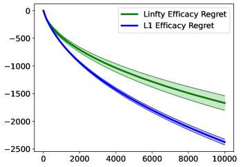
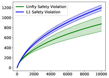
Figure 7: Comparison of $L_{\infty}$ vs $L_{1}$ relaxations of DOSLB over 30 runs on the isntance of Example 9. Observe that the $L_{1}$ relaxation yields more aggressive, and less safe play.