Maximal Masses of White Dwarfs for Polytropes in $R^{2}$ Gravity and Theoretical Constraints

Abstract

We examine the Chandrasekhar limit for white dwarfs in $f(R)$ gravity, with a simple polytropic equation of state describing stellar matter. We use the most popular $f(R)$ gravity model, namely the $f(R)=R+\alpha R^{2}$ gravity, and calculate the parameters of the stellar configurations with polytropic equation of state of the form $p=K\rho^{1+1/n}$ for various values of the parameter $n$. In order to simplify our analysis we use the equivalent Einstein frame form of $R^{2}$-gravity which is basically a scalar-tensor theory with well-known potential for the scalar field. In this description one can use simple approximations for the scalar field $\phi$ leaving only the potential term for it. Our analysis indicates that for the non-relativistic case with $n=3/2$, discrepancies between the $R^{2}$-gravity and General Relativity can appear only when the parameter $\alpha$ of the $R^{2}$ term, takes values close to maximal limit derived from the binary pulsar data namely $\alpha_{max}=5\times 10^{15}$ cm². Thus, the study of low-mass white dwarfs can hardly give restrictions on the parameter $\alpha$. For relativistic polytropes with $n=3$ we found that Chandrasekhar limit can in principle change for smaller $\alpha$ values. The main conclusion from our calculations is the existence of white dwarfs with large masses $\sim 1.33M_{\odot}$, which can impose more strict limits on the parameter $\alpha$ for the $R^{2}$ gravity model. Specifically, our estimations on the parameter $\alpha$ of the $R^{2}$ model is $\alpha\sim 10^{13}$ cm².

I Introduction

The accelerated expansion of the Universe [1, 2, 3] has been confirmed by various observations from moment of its discovering in 1998. Apart from data based on standard candles, these observations include of data for cosmic microwave background anisotropy [4], shear due to the gravitational weak lensing [5], data about absorption lines in Lyman-a-forest [6] and others. Now the question is what causes the late-time cosmological acceleration. To date, there no clear answer exists on this issue, and this question remains one of the puzzles in cosmology and theoretical physics. One solution for this late-time acceleration problem is based on the assumption that the Universe contains some non-standard cosmic fluid with negative pressure. This fluid (dark energy) is distributed in the Universe homogeneously. In the simplest approach, the dark energy is nothing else than the vacuum energy (or cosmological constant). For a satisfactory agreement with observational data density of vacuum energy should be nearly 72% of the global energy budget of the Universe. Only 4 % of Universe energy consists of baryonic matter. The remaining 24% is cold dark matter (CDM) which is also mysterious in its nature. Various unknown hypothetical particles could constitute this “dark sector” of the Universe, for example weakly interacting massive particles or/and axions or axion-like particles.

To date, the most successful model for the late-time evolution of the Universe is the $\Lambda$-Cold-Dark-Matter ($\Lambda$CDM) model. Although standard cosmology describes observational data with high precision, it has several shortcomings, from a theoretical viewpoint. If the cosmological constant constitutes the “vacuum state” of the gravitational field, one need have to explain the very large discrepancy of the magnitude between its observed value at a cosmological level and the one predicted by any quantum field theories [7]. This discrepancy is also known as the cosmological constant problem, which is one of the most fundamental problems of the $\Lambda$CDM model. Apart from this theoretical problem, if one sticks with the standard General Relativity (GR) description of late-time and uses scalar fields to describe the late-time evolution, the slightly phantom nature allowed by the observational data, makes the GR description unappealing, since tachyons are needed in order to successfully describe the slightly phantom evolution. Another appealing theoretical description of the dark energy era is offered by modified gravity in its various forms [8, 9, 10, 11, 12, 13, 14], which extend GR directly. Modified gravity theories have the advantage of describing successfully and in a minimal way the late-time era without the use of phantom scalars, and in many cases, the unification of the inflationary era with the early-time acceleration is achieved. However, when considering modifications of GR, a holistic approach compels to consider not only possible manifestations of such theories at a cosmological level, but also at an relativistic astrophysical level, also because strong gravitational regimes could be considered if GR is the weak field limit of some more complicated effective gravitational theory.

Usually in this context, neutron stars (NSs) serve as the perfect candidates for studying modified gravity effects at an astrophysical level, and in the literature there exist various works in this research line, see for example, [15, 16, 17, 18, 19, 20, 21, 22, 23, 24, 25, 26, 27], and for a recent review see [28]. For a simple $R^{2}$ gravity, the calculations indicate that the effective gravitational mass of NSs increases although the value of such increase is not large. The scalar curvature $R$ outside the NS doesn’t drop to zero as for for the Schwarzschild solution in GR, but asymptotically approaches zero at the spatial (and from a calculational point of view at the numerical) infinity. The gravitational mass parameter at the star surface decreases in comparison with GR for same density of nuclear matter at the center of star, but contributions to the gravitational mass are obtained from regions beyond the surface of the star, at which $R\neq 0$, thus the net result is a total increase of the gravitational mass. This effect in NSs may explain in an appealing way the hyperon problem and having soft equations of state with large NSs masses, beyond the stretch of GR limits.

This interesting result can provide a clear cut description for large mass NSs [29, 30, 31, 32, 33, 34, 35, 24, 25, 26]. In light of the relatively recent GW190814 event, modified gravity serves as a cutting edge probable description of nature in limits where GR needs to be supplemented by a Occam’s razor compatible theory. Indeed, solutions such as strange stars, rely on QCD, which directly changes the physics of hydrodynamic equilibrium of compact stellar objects. Modified gravity on the other hand does not change the way of thinking for relativistic objects, just changes the gravitational theory which controls the hydrodynamic equilibrium.

From the above line of reasoning, in this work we consider another class of compact objects, namely white dwarfs. White dwarfs are usually the final state of evolution for stars with masses up to 8 - 10.5 $M_{\odot}$ [36]. After the hydrogen-fusing period of a main-sequence star ends, star will expand to a red giant. Due to the $\alpha$-process helium fuses to carbon and oxygen. For low and medium star masses core temperature is insufficient to fuse carbon and after shedding of outer layers remnant composed of carbon and oxygen forms. For main-sequence stars with more large masses (in range of 8-10.5 $M_{\odot}$, the core temperature will exceed $10^{9}$ K and carbon fuses but not neon. In this case oxygen–neon–magnesium white dwarf remains [37]. Also helium white dwarfs can forms due to mass loss in binary systems [38].

Electron degeneracy pressure supports a white dwarf in equilibrium. One of the consequence of this is the existence of a limit for mass of white dwarf which cannot be exceeded without collapsing to a neutron star This value is known as Chandrasekhar limit [39]. For a non-rotating white dwarf maximal mass is approximately $5.7M_{\odot}/\mu_{e}^{2}$, where $\mu_{e}$ is the average molecular weight per electron of the star. It is interesting to consider question about Chandrasekhar limit in modified gravity theories.

The authors of Ref. [40] considered the model $f(R)=R+\alpha R^{2}(1+\gamma R)$ and obtained for very large range of values of the parameters $\alpha$ and $\gamma$ ($\gamma=4\times 10^{16}$ cm²) a considerable increase of the Chandrasekhar limit for white dwarfs (up to $2.95M_{\odot}$). This result is interesting but the existence of such white dwarfs is not confirmed by observational data. More realistic models of white dwarfs in Palatini $f(R)$ gravity (in such approach there is no extra degree of freedom for the gravitational sector) are investigated in Refs. [41, 42]. Although the central densities of white dwarfs are not so large as in the cores of NSs, one can expect that effects of modified gravity would take place due to the larger radii of white dwarfs (in principle one can say about “cumulative effects”). Our calculations confirm this conclusion. We start off with the usual equations describing non-rotating star in equilibrium and we use the Lane-Emden equation for matter with a polytropic equation of state. In GR one already needs to consider the Tolman-Oppenheimer-Volkoff (TOV) equations. For white dwarfs, the relativistic effects are negligible of course, but it is interesting to compare these corrections with possible influences of modified gravity. This is the main reason for which we consider these equations. The next step is to investigate solutions for equations describing star configuration in $R^{2}$ gravity. Besides the mass parameter, the density and pressure in $f(R)$ gravity, another independent variable arises, namely the scalar curvature. In GR for non-rotating stars, the scalar curvature is defined by trace of energy-momentum tensor. But in $f(R)$ gravity the scalar curvature should be also considered when studying the dynamical equilibrium.

We consider simple polytropic equations of state for matter, of the form, $p=K\rho^{1+1/n}$ describing the white dwarfs. For non-relativistic electrons, the index of the polytrope is $n=3/2$, and for relativistic ones, the index is $n=3$. For our analysis it is useful to consider the equivalent Brans-Dicke theory with a scalar field. Assuming that the derivatives of the scalar field are negligible, in comparison with potential term, one obtains simple equations which are similar to the TOV equations, but with additional terms for the pressure and the density. The net effect of this scalar field is that it reduces the gravitational mass and simultaneously increases the radius of the stellar configuration.

II The Lane-Emden Equation and the TOV Equations

The hydrodynamic equilibrium of non-rotating stars in Newtonian gravity is described by the following well-known equations (hereinafter we use Geometrized units in which $c=G=1$):

$$\frac{dm}{dr}=4\pi r^{2}\rho,$$ (1)

$$\frac{dp}{dr}=-\frac{m\rho}{r^{2}},$$ (2)

where $\rho$ and $p$ are the density and the pressure of stellar matter respectively. For white dwarfs, one can use polytropic equation of state of the form,

$$p=K\rho^{1+1/n}\,,$$ (3)

where $K$, $n$ are constants. We assume that the speed of light is $c=1$ and therefore pressure and density have the same dimensions. In this case, it is useful to define the following dimensionless functions $\theta$ and $\mu$ and the coordinate variable $x$:

$$\rho=\rho_{c}\theta^{n},\quad m=\mu\rho_{c}a^{3},\quad r=ax,$$

$$a=\left(\frac{(n+1)K\rho_{c}^{1/n-1}}{4\pi}\right)^{1/2}.$$

In terms of dimensionless variables, Eqs. (1), (2) are rewritten in the following way

$$\frac{d\mu}{dx}=4\pi x^{2}\theta^{n},$$ (4)

$$\frac{d\theta}{dx}=-\frac{\mu}{4\pi x^{2}}.$$ (5)

These equations are equivalent to well-known Lane-Emden equation,

$$\frac{1}{x^{2}}\frac{d}{dx}\left(x^{2}\frac{d\theta}{dx}\right)=-\theta^{n}.$$ (6)

For more exact description one need to account relativistic theory of gravity, in which case one needs to replace Eqs. (1) and (2) by the TOV equations,

$$\frac{dm}{dr}=4\pi\rho r^{2},$$ (7)

$$\frac{dp}{dr}=-(\rho+p)\frac{m+4\pi pr^{3}}{r^{2}\left(1-\frac{2m}{r}\right)}.$$ (8)

The second equation for the polytropic EoS and variables $\mu$, $\theta$ can be reduced to,

$$\frac{1}{1+4\pi\beta\theta/(n+1)}\frac{d\theta}{dx}=-\frac{1}{4\pi}\frac{\mu+16\pi^{2}(n+1)^{-1}x^{3}\beta\theta^{n+1}}{x(x-2\beta\mu)}.$$ (9)

The equation for the gravitational parameter $\mu$ remains the same. Here $\beta$ is a dimensionless small parameter,

$$\beta=\rho_{c}a^{2}=\frac{n+1}{4\pi}K\rho_{c}^{1/n}<<1\,,$$

for typical densities at the center of white dwarfs. Up to densities $10^{6}$ g/cm³ one can use polytropic equation with $n=3/2$ and,

$$K=1.0036\times 10^{13}/\mu_{e}^{5/3}\,,$$

in CGS-system. Here $\mu_{e}$ is average molecular weight per one electron. We considered $\mu_{e}=2$. One can solve the equations (5) and (9) numerically and obtain physical parameters of polytropes, that is the mass and radius.

The integration of the Lane-Emden equation for $n=3/2$ gives that for $x=x_{f}=3.653$ $\theta(x_{f})=0$ and $\mu(x_{f})=34.106$. These results change in GR, but are quantitatively negligible. In Fig. 1 we present the corresponding relation between the mass, radius and the central density of the stellar configurations for central densities between $10^{5}$ and $10^{6}$ $\mbox{g/cm}^{3}$.

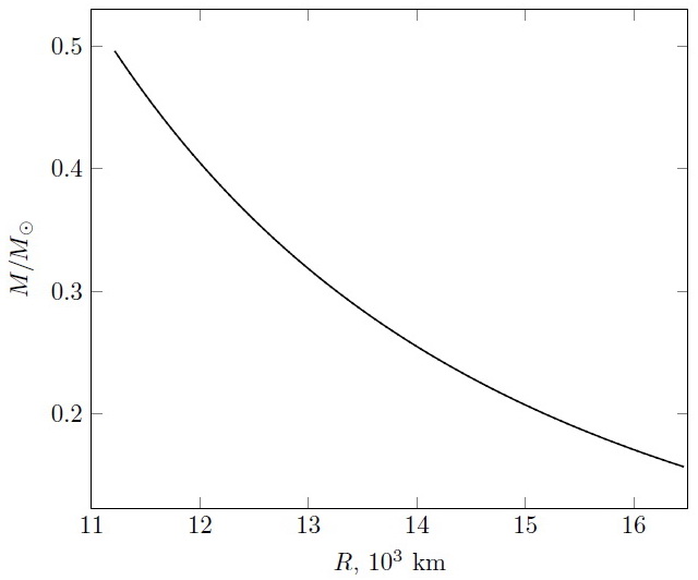
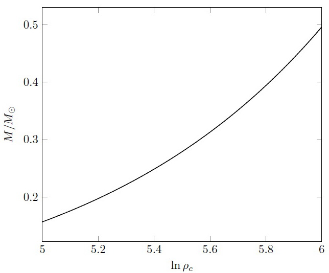
Figure 1: Mass-radius and mass-central density diagrams for stellar configurations with $n=3/2$.

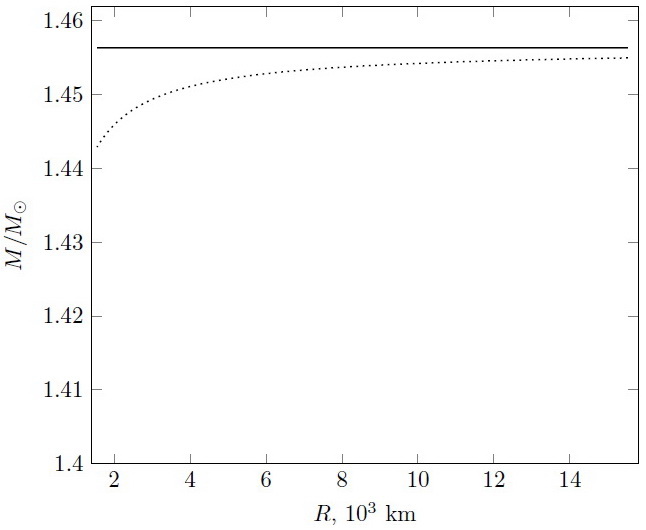
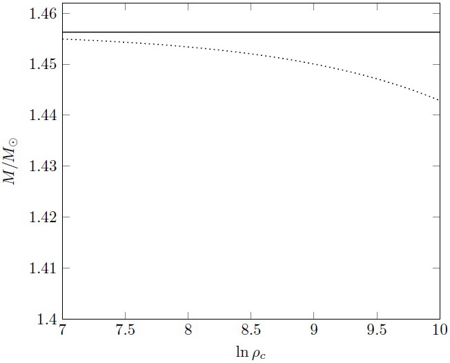
Figure 2: Mass-radius and mass-central density diagrams for polytropic stellar configurations with index $n=3$. The solid and dotted lines correspond to solution of Lane-Emden equation and relativistic Eqs. (4), (9) correspondingly.

For relativistic densities ($\rho>>10^{6}$ g/cm³), stellar matter in white dwarfs can be described by polytropic equations with $n=3$. The parameter $K$ in this case is,

$$K=1.2435\times 10^{15}/\mu_{e}^{4/3}\quad\mbox{CGS}.$$

For the case $n=3$, the mass of star does not depend on the central density and $\mu(x_{f})=25.362$ for $x_{f}=6.896$ in Geometrized units. This corresponds to the Chandrasekhar limit $M=1.456M_{\odot}$. The relativistic effects again slightly change this result (see Fig. 2). Now we investigate how these results change in modified gravity.

III Spherically symmetric stellar configurations in f(R)-gravity

For $f(R)$ gravity the standard Einstein-Hilbert action with scalar curvature $R$ is replaced by the following:

$$S=\frac{1}{16\pi}\int d^{4}x\sqrt{-g}f(R)+S_{{\rm matter}},$$ (10)

where $g$ is determinant of the metric $g_{\mu\nu}$ and $S_{\rm matter}$ is the action of the standard perfect fluid matter.

The spherically symmetric spacetime that describes the non-rotating star has the following form,

$$ds^{2}=-e^{2\psi}dt^{2}+e^{2\lambda}dr^{2}+r^{2}d\Omega^{2}.$$ (11)

Here $\psi$ and $\lambda$ are two independent functions of the radial coordinate. Varying the action with respect to metric tensor elements gives the Einstein equation in $f(R)$ gravity:

$$f^{\prime}(R)G_{\mu\nu}-\frac{1}{2}(f(R)-f^{\prime}(R)R)g_{\mu\nu}-(\nabla_{\mu}\nabla_{\nu}-g_{\mu\nu}\Box)f^{\prime}(R)=8\pi T_{\mu\nu}.$$ (12)

Here $G_{\mu\nu}=R_{\mu\nu}-\frac{1}{2}Rg_{\mu\nu}$ is the Einstein tensor, comma means derivative on argument of function $f(R)$ and $T_{\mu\nu}$ is the energy–momentum tensor. For perfect fluid components of $T_{\mu\nu}$ is $T_{\mu\nu}\mbox{diag}(e^{2\psi}\rho,e^{2\lambda}p,r^{2}p,r^{2}\sin^{2}\theta p)$. The components of (12) yield the TOV equations in frames of $f(R)$ gravity, and explicitly have the following form:

$$\frac{f^{\prime}(R)}{r^{2}}\frac{d}{dr}\left[r\left(1-e^{-2\lambda}\right)\right]=8\pi\rho+\frac{1}{2}\left(f^{\prime}(R)R-f(R)\right)+e^{-2\lambda}\left[\left(\frac{2}{r}-\frac{d\lambda}{dr}\right)\frac{df^{\prime}(R)}{dr}+\frac{d^{2}f^{\prime}(R)}{dr^{2}}\right]$$ (13)

$$\frac{f^{\prime}(R)}{r}\left[2e^{-2\lambda}\frac{d\psi}{dr}-\frac{1}{r}\left(1-e^{-2\lambda}\right)\right]=8\pi p+\frac{1}{2}\left(f^{\prime}(R)R-f(R)\right)+e^{-2\lambda}\left(\frac{2}{r}+\frac{d\psi}{dr}\right)\frac{df^{\prime}(R)}{dr}$$ (14)

The third equation can be obtained from the conservation law of the energy-momentum tensor

$$\nabla^{\mu}T_{\mu\nu}=0$$

and gives,

$$\frac{dp}{dr}=-(\rho+p)\frac{d\psi}{dr}.$$ (15)

The equation for the scalar curvature $R$ can be obtained by taking of the trace of (12). We have for $R=R(r)$ the following equation:

$$3\triangle_{r}(f(R)-R)+f^{\prime}(R)R-2f(R)=-{8\pi}(\rho-3p),$$ (16)

where $\triangle_{r}$ is radial part of the 3-dimensional Laplace operator for metric (11),

$$e^{2\lambda}\triangle_{r}=\frac{d^{2}}{dr^{2}}+\left(\frac{2}{r}+\frac{d\psi}{dr}-\frac{d\lambda}{dr}\right)\frac{d}{dr}.$$

One needs to solve Eqs. (13), (14) outside the star with $\rho=p=0$. At the surface of star ($r=r_{s}$, $\rho=p=0$), the junction conditions should be satisfied,

$$\lambda_{in}(r_{s})=\lambda_{out}(r_{s}),\quad R_{in}(r_{s})=R_{out}(r_{s}),\quad R^{\prime}_{in}(r_{s})=R^{\prime}_{out}(r_{s}).$$

The gravitational mass parameter $m(r)$ is defined from $\lambda$ through the following relation,

$$e^{-2\lambda}=1-\frac{2m}{r}.$$ (17)

The asymptotic flatness requirement gives the constraint on scalar curvature and mass parameter,

$$\lim_{r\rightarrow\infty}R(r)=0,\lim_{r\rightarrow\infty}m(r)=\mbox{const}.$$

IV Equivalent Scalar-Tensor Theory

It is useful to consider the description of the $f(R)$ gravity stellar configuration in terms of the corresponding scalar-tensor theory. For such a theory, the difference between the resulting equations and (7), (8) for polytropes is more transparent. In the end for the construction of the $M-R$ graphs we shall use the Jordan frame transformed expressions for the mass and radii. For $f(R)$ gravity, the equivalent Brans-Dicke theory with scalar field $\Phi$ has the following action,

$$S_{g}=\frac{1}{16\pi}\int d^{4}x\sqrt{-g}\left(\Phi R-U(\Phi)\right).$$ (18)

Here the scalar field is $\Phi=f^{\prime}(R)$ and the potential is $U(\Phi)=Rf^{\prime}(R)-f(R)$. The transformation $\tilde{g}_{\mu\nu}=\Phi g_{\mu\nu}$ for coordinates allows to write the action in the Einstein frame

$$S_{g}=\frac{1}{16\pi}\int d^{4}x\sqrt{-\tilde{g}}\left(\tilde{R}-2\tilde{g}^{\mu\nu}\partial_{\mu}\phi\partial_{\nu}\phi-4V(\phi)\right),$$ (19)

where $\phi=\sqrt{3}\ln\Phi/2$ and the redefined potential in the Einstein frame $V(\phi)$ is $V(\phi)=\Phi^{-2}(\phi)U(\Phi(\phi))/4$. For redefined spacetime metrics, we take the expression which formally coincides with (11), but with different functions $\tilde{\psi}$ and $\tilde{\lambda}$, that is,

$$d\tilde{s}^{2}=\Phi ds^{2}=-e^{2\tilde{\psi}}dt^{2}+e^{2\tilde{\phi}}\tilde{dr}^{2}+\tilde{r}^{2}d\Omega^{2}.$$ (20)

In Eq. (20) we have $\tilde{r}^{2}=\Phi r^{2}$, $e^{2\tilde{\psi}}=\Phi e^{2\psi}$ and from the equality

$$\Phi e^{2\lambda}dr^{2}=e^{2\tilde{\lambda}}d\tilde{r}^{2}$$

it follows that,

$$e^{-2\lambda}=e^{-2\tilde{\lambda}}\left(1-\tilde{r}\phi^{\prime}(\tilde{r})/\sqrt{3}\right)^{2}.$$

Therefore, the mass parameter $m(r)$ can be obtained from $\tilde{m}(\tilde{r})$ as

$$m(\tilde{r})=\frac{\tilde{r}}{2}\left(1-\left(1-\frac{2\tilde{m}}{\tilde{r}}\right)\left(1-\tilde{r}\phi^{\prime}(\tilde{r})/\sqrt{3}\right)^{2}\right)e^{-\phi/\sqrt{3}}$$ (21)

The resulting equations for the metric functions $\tilde{\lambda}$ and $\tilde{\psi}$ is very similar to the TOV equations with redefined energy and pressure, and with additional terms with the energy density and pressure of the scalar field $\phi$ being:

$$\frac{1}{\tilde{r}^{2}}\frac{d\tilde{m}}{d\tilde{r}}=4\pi e^{-4\phi/\sqrt{3}}\rho+\frac{1}{2}\left(1-\frac{2\tilde{m}}{\tilde{r}}\right)\left(\frac{d\phi}{d\tilde{r}}\right)^{2}+V(\phi),$$ (22)

$$\frac{1}{p+\rho}\frac{dp}{d\tilde{r}}=-\frac{\tilde{m}+4\pi e^{-4\phi/\sqrt{3}}p\tilde{r}^{3}}{\tilde{r}(\tilde{r}-2\tilde{m})}-\frac{\tilde{r}}{2}\left(\frac{d\phi}{d\tilde{r}}\right)^{2}+\frac{\tilde{r}^{2}V(\phi)}{\tilde{r}-2\tilde{m}}+\frac{1}{\sqrt{3}}\frac{d\phi}{d\tilde{r}},$$ (23)

The hydrostatic equilibrium condition is rewritten as,

$$\frac{dp}{d\tilde{r}}=-(\rho+p)\left(\frac{d\psi}{d\tilde{r}}-\frac{1}{\sqrt{3}}\frac{d\phi}{d\tilde{r}}\right).$$ (24)

Finally the last equation of motion for scalar field is equivalent to Eq. (16) in $f(R)$ theory:

$$\triangle_{\tilde{r}}\phi-\frac{dV(\phi)}{d\phi}=-\frac{4\pi}{\sqrt{3}}e^{-4\phi/\sqrt{3}}(\rho-3p).$$ (25)

The potential $V(\phi)$ can be written in explicit form only for simple $f(R)$ models. For example for $f(R)=R+\alpha R^{2}$ one can obtain that,

$$V(\phi)=\frac{1}{16\alpha}\left(1-e^{-2\phi/\sqrt{3}}\right)^{2}.$$ (26)

For simple power-law models of the form $f(R)=R+\alpha R^{m}$ we have,

$$V(\Phi)=D\Phi^{-2}\left(\Phi-1\right)^{\frac{m}{m-1}},\quad D=\frac{m-1}{m^{\frac{m}{m-1}}}\alpha^{\frac{1}{1-m}},\quad\Phi=e^{2\phi/\sqrt{3}}.$$ (27)

Passing to dimensionless variables $\tilde{\mu}$ and $\theta$ we obtain the following equations,

$$\frac{d\tilde{\mu}}{dx}=4\pi\tilde{x}^{2}\theta^{n}\mathrm{e}^{-4\phi/\sqrt{3}}+\frac{\tilde{x}^{2}}{\beta}\left(\frac{1}{2}\left(1-\frac{2\beta\tilde{\mu}}{\tilde{x}}\right)\left(\frac{d\phi}{d\tilde{x}}\right)^{2}+v(\phi)\right),$$ (28)

$$\frac{1}{1+4\pi\beta\theta/(n+1)}\frac{d\theta}{d\tilde{x}}=-\frac{1}{4\pi}\frac{\tilde{\mu}+16\pi^{2}\beta\theta^{n+1}\tilde{x}^{3}e^{-4\phi/\sqrt{3}}}{\tilde{x}(\tilde{x}-2\tilde{\beta}\tilde{\mu})}-$$ (29)

$$-\frac{\tilde{x}^{2}}{4\pi\beta(\tilde{x}-2\beta\tilde{\mu})}\left(\frac{1}{2}\left(1-\frac{2\beta\tilde{\mu}}{\tilde{x}}\right)\left(\frac{d\phi}{d\tilde{x}}\right)^{2}-v(\phi)\right)+\frac{1}{4\sqrt{3}\pi\beta}\frac{d\phi}{d\tilde{x}}$$

Here we introduced the dimensionless potential $v(\phi)$,

$$v(\phi)=a^{2}V(\phi).$$

The equation for scalar field $\phi$ after some calculations can be written in the following form,

$$\left(1-\frac{2\beta\tilde{\mu}}{\tilde{x}}\right)\left(\frac{d^{2}\phi}{d\tilde{x}^{2}}+\left(\frac{2}{\tilde{x}}-\frac{4\pi\beta}{1+4\pi\beta/(n+1)}\frac{d\theta}{d\tilde{x}}+\frac{1}{\sqrt{3}}\frac{d\phi}{d\tilde{x}}\right)\frac{d\phi}{d\tilde{x}}\right)+$$ (30)

$$+\left(\frac{\beta\tilde{\mu}}{\tilde{x}^{2}}-\frac{\beta}{\tilde{x}}\frac{d\tilde{\mu}}{d\tilde{x}}\right)\frac{d\phi}{d\tilde{x}}-\frac{dv}{d\phi}=-\frac{4\pi\beta}{\sqrt{3}}e^{-4\phi/\sqrt{3}}\theta^{n}\left(1-12\pi\beta\theta/(n+1)\right).$$

Equations (28), (29) with (30) can be solved numerically for various values of the parameter $n$. One needs to impose following conditions at $\tilde{x}=0$ for the numerical integration,

$$\theta(0)=1,\quad\tilde{\mu}(0)=0,\quad\phi(0)=\phi_{0},\quad\frac{d\phi}{d\tilde{x}}=0.$$

The condition for $\phi_{0}$ should correspond to a solution with flat asymptotic behavior at spatial infinity (numerical infinity), that is,

$$\phi\rightarrow 0\quad\mbox{at}\quad x\rightarrow\infty.$$

It is convenient to analyse system of equations in Einstein frame and then after calculations go back to Jordan frame.

V Perturbative Analysis of the Solution

For $R^{2}$ gravity, the potential in Geometrized units is,

$$v(\phi)=\frac{1}{16\tilde{\alpha}}\left(1-e^{-2\phi/\sqrt{3}}\right)^{2},\quad\tilde{\alpha}=\alpha/a^{2}.$$ (31)

The authors of Ref. [43] estimated the upper limit for $\alpha$ as $\sim 5\times 10^{15}$ cm² from binary pulsar data. For $n=3/2$ scale $a$ varies from $3\times 10^{8}$ cm to $4.5\times 10^{8}$ cm (for central densities $10^{5}<\rho_{c}<10^{6}$ g/cm³. The value of scalar field is very small and therefore one can use Taylor expansion for the potential leaving only the first non-zero term:

$$v(\phi)=\frac{\phi^{2}}{12\tilde{\alpha}}.$$

Since the parameter $\alpha/a^{2}$ is negligible, one can expect that the potential term $v(\phi)$ is very large in comparison with kinetic term $(d\phi/d\tilde{x})^{2}$ and we may omit these terms in the right hand side of Eqs. (28), (29). Considering Eq. (30) in this context one can neglect derivatives of scalar field in comparison with term $dv/d\phi\sim\phi$. In the right hand side of Eq. (30) we leave only zero term for exponent (since $\beta$ is already a small parameter) and in effect we obtain the following relation for the scalar field,

$$\frac{\phi}{6\tilde{\alpha}}=\frac{4\pi\beta}{\sqrt{3}}\theta^{n}\left(1-12\pi\beta\theta/(n+1)\right).$$ (32)

Keeping in Eq. (29) the last term with first derivative for scalar field and potential terms which $\sim\tilde{\alpha}$, we will integrate equations Eqs. (28), (29) for polytropic EoSs with $n=3/2$ and $n=3$ and we shall compare the results with Newtonian gravity and General Relativity. If the approximation (32) is valid, then the scalar field at the surface of the star is zero and the gravitational mass parameter $\tilde{m}$ coincides with $m$ at the star surface $r=\tilde{r}=R_{s}$ where $R_{s}$ is the radius of star.

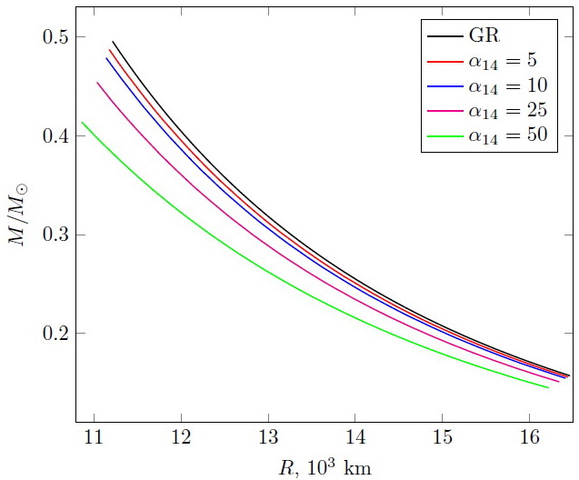
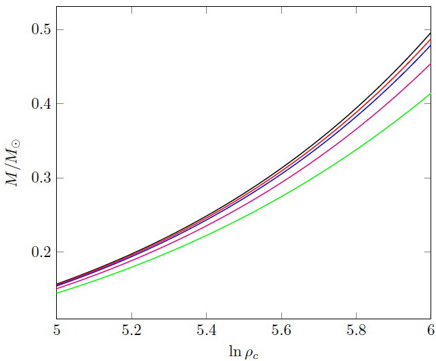
Figure 3: Mass-radius and mass-central density diagrams for stellar configurations with $n=3/2$ for various $\alpha$ (symbol $\alpha_{n}$ hereinafter means that $\alpha$ is given in units of $10^{n}$ cm²) in comparison with General Relativity.

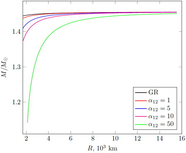
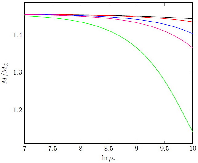
Figure 4: Mass-radius and mass-central density diagrams for stellar configurations with $n=3$ in scalar-tensor gravity for various $\alpha$ in comparison with General Relativity.

$\alpha_{12}$	$M,$	$R_{s},$	$\alpha$	$M,$	$R_{s},$	$\alpha$	$M,$	$R_{s},$	$\alpha_{12}$	$M,$	$R_{s},$
	$M_{\odot}$	km		$M_{\odot}$	km		$M_{\odot}$	km		$M_{\odot}$	km
$\rho_{c}=10^{7}$ g/cm3			$\rho_{c}=10^{8}$ g/cm3			$\rho_{c}=10^{9}$ g/cm3			$\rho_{c}=10^{10}$ g/cm3
0	1.455	15530	0	1.453	7210	0	1.450	3340	0	1.443	1550
1	1.455	15530	1	1.453	7210	1	1.448	3350	1	1.435	1560
5	1.455	15530	5	1.451	7210	5	1.441	3360	5	1.403	1590
10	1.454	15530	10	1.450	7220	10	1.432	3380	10	1.365	1630
50	1.451	15560	50	1.434	7280	50	1.366	3520	50	1.142	2110

Table 1: Masses and radii of stellar configurations at different values of central density and $\alpha$ for $n=3$.

We calculated the relation between the mass and radius in the same interval of the central density for $n=3/2$ as in the case of GR, using the Jordan frame transformed quantities under study. Our calculations indicate that only when the parameter $\alpha$ takes values close to the upper limit of [43], significant deviations from GR occur. In Fig. 3 we present the mass-radius relation and the dependence of the mass from the central density in comparison with the GR results. For a given mass, the radius of the star decreases. Of course these results do not allow us having hopes for pinpointing the underlying extended gravity theory from real white dwarf observational data. The corresponding errors of measurements for masses and radii have the same order as the effect from $R^{2}$-gravity even for maximal values of the parameter $\alpha$.

For $n=3$ and with the interval of the central densities being between $10^{7}$ and $10^{10}$ g/cm³, already for smaller values of the parameter $\alpha$, the mass-radius diagram deviates from the straight line corresponding to Chandrasekhar limit (see Fig. 4). For a given central density, the radius of star increases in comparison with the radius in the case of GR. The parameters of the stellar configurations for some central densities are given in Table 1.

It is also interesting to investigate the mass and density profiles in comparison with the GR results. From Fig. 5 one can see that the effect from modified gravity is cumulative. Density profiles in modified gravity and GR differ negligible but the total mass inside a radius $r$, gradually decreases. One note that results on Fig. 5 are given for $m$ as function of $r$ in Jordan frame.

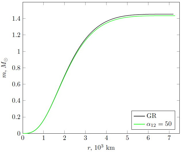
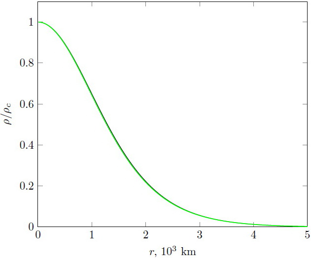
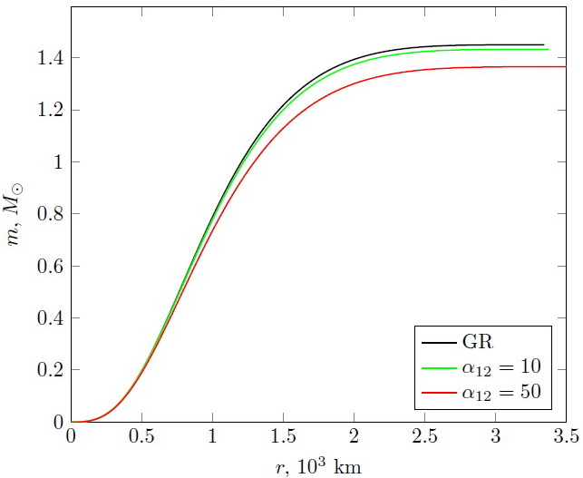
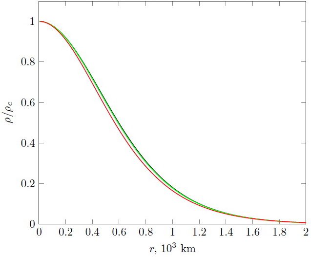
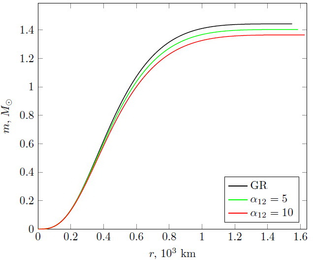
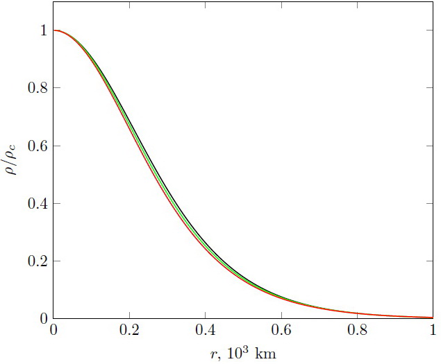
Figure 5: Profiles of the mass parameter in Jordan frame and density for $\rho_{c}=10^{8}$ g/cm³ (upper panel), $\rho_{c}=10^{9}$ g/cm³ (middle panel), $\rho_{c}=10^{10}$ g/cm³ (bottom panel) for some $\alpha$ in units of $10^{12}$ cm² for $n=3$. For better visibility we cut r-axis for coordinates where $\rho/\rho_{c}$ is negligible.

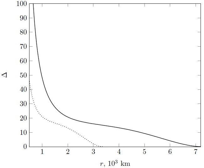
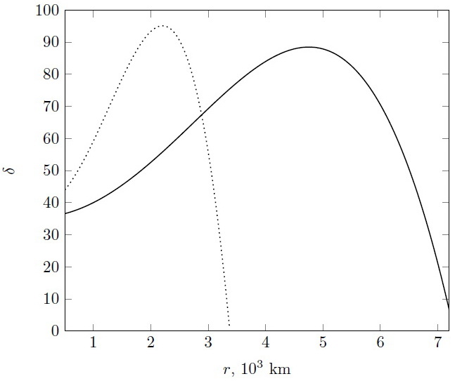
Figure 6: The relation between kinetic and potential terms $\Delta=2{v}/{\phi^{\prime 2}}$ (left) for $\rho_{c}=10^{8}$ g/cm³, $\alpha=5\times 10^{13}$ cm² (solid line) and $\rho_{c}=10^{9}$ g/cm³, $\alpha=10^{13}$ cm² (dotted line). On the right panel, the ratio $\delta=\frac{v}{\phi^{\prime}/x}$ is shown.

The final step is the analysis of applicability of the perturbative approach. For illustration we compared values of potential $v$ and the term with the square of the derivative of field $\phi$ for some parameters (Fig. 6). Only in the vicinity of star’s surface, the term $\phi^{\prime 2}/2$ is comparable with $v(\phi)$, but near the star surface, the effects of modified gravity in any case are negligible. We also investigated relation between $v(\phi)$ and term $\phi^{\prime}/x$ in equation of scalar field. Calculation therefore indicates that the simple approximation (31) is valid for the scalar field $\phi$ and the values of the parameters considered in this paper.

VI Concluding Remarks

For neutron stars in $R^{2}$-gravity, the maximal mass for $\alpha\sim 10^{11}$ cm² increases by a value around $\delta M\sim 0.05-0.09$ $M_{\odot}$ ($\delta M$ depends from equation of state for dense matter, see [44]). The densities in neutron star cores for maximal masses are $\rho_{c}>3\times 10^{15}$ g/cm³.

For relativistic polytropes in white dwarfs we obtain the same order effects (but mass decreases) for central densities $\sim 10^{10}$ g/cm³ (five orders of magnitude difference) although for $\alpha$, we obtain two orders of magnitude larger ($\sim 10^{13}$ cm²). This feature can be explained by the fact that the characteristic size of white dwarfs is three orders greater in comparison with neutron star. Additional terms in modified TOV equations are smaller in comparison with NSs case, but due to the long distance we obtain comparable effect.

It is interesting to note that our results concerning relativistic polytropes are in concordance with calculations for NSs with $M<1.5M_{\odot}$. For densities $\rho_{c}<10^{15}$ g/cm³, the mass of the NSs in $R^{2}$ gravity decreases in comparison with the GR case. This result can be explained by the stiffness of dense matter EoS which decreases with density. One can conclude that only for very large densities, the net effect of $R^{2}$ gravity yields an increase of the gravitational mass. Although for more precise calculations of white dwarfs parameters in $R^{2}$ gravity one should consider more realistic EoS than polytropic ones, we can expect that the main result of this work will remain the same: the mass of the white dwarf decreases in comparison with GR.

Our results can be useful for establishing more stringent limits on $R^{2}$ gravity. Now according to observations there are white dwarf stars with masses larger than $1.3M_{\odot}$. According to [45] 25 such white dwarfs in vicinity of Sun System exist. From realistic carbon monoxide core model the highest mass of white dwarf is $1.334M_{\odot}$ which corresponds to the high-density limit $\rho=10^{9}$ g/cm³ (in GR). White dwarf J1329 + 2549 is currently the most massive white dwarf known in the solar neighborhood with well-constrained atmospheric parameters and a mass of $1.351\pm 0.006M_{\odot}$. These results lead to conclusion that GR gives satisfactory picture for white dwarfs parameters.

At first glance, this issue does not allow us to constrain significantly $R^{2}$ gravity. But we can impose restrictions on the parameter $\alpha$. The assumption that central density of ultra-massive white dwarfs is around $10^{9}$ g/cm³ and that decreasing of mass due to the modification of gravity is the same as in a case of relativistic polytrope for $\rho_{c}=10^{9}$ g/cm³, allow us to draw the following conclusion.: for $\alpha\sim 5\times 10^{13}$ cm² existence of white dwarfs with CO cores and masses larger than $1.3M_{\odot}$ would be questionable. Unlike neutron stars, the EoS for matter in white dwarfs is considered more well established and it is difficult to propose realistic EoS which describes in GR white dwarfs with masses $>1.33M_{\odot}$. Therefore in principle we can estimate upper limit on $\alpha$ as $\sim 10^{13}$ cm².

This is a quite interesting situation. From observational data for white dwarf we obtained upper limit of an unknown modified gravity parameter. On the contrary some indications to favor of possible existence of supermassive NS with $M>2.2M_{\odot}$ allow us to estimate the lower limit of $\alpha$ although for dense nuclear matter, the uncertainty in knowledge of the exact EoS is large enough. Thus for testing modified gravity it is useful to consider not only NSs but also less extreme objects like white dwarfs.

References

- [1] S. Perlmutter et al. [Supernova Cosmology Project Collaboration], Astrophys. J. 517, 565 (1999) [arXiv:astro-ph/9812133].
- [2] A. G. Riess et al. [Supernova Search Team Collaboration], Astron. J. 116, 1009 (1998) [arXiv:astro-ph/9805201].
- [3] A. G. Riess et al. [Supernova Search Team Collaboration], Astrophys. J. 607, 665 (2004)[arXiv:astro-ph/0402512].
- [4] D. N. Spergel et al. [WMAP Collaboration], Astrophys. J. Suppl. 148, 175 (2003) [arXiv:astro-ph/0302209].
- [5] C. Schimdt et al., Astron. Astrophys. 463, 405 (2007).
- [6] P. McDonald et al., Astrophys. J. Suppl. 163, 80 (2006).
- [7] S. Weinberg, Rev. Mod. Phys. 61, 1 (1989).
- [8] S. Nojiri, S. D. Odintsov and V. K. Oikonomou, Phys. Rept. 692 (2017) 1 [arXiv:1705.11098 [gr-qc]].
- [9] S. Nojiri, S.D. Odintsov, Phys. Rept. 505, 59 (2011);
- [10] S. Capozziello, M. De Laurentis, Phys. Rept. 509, 167 (2011) [arXiv:1108.6266 [gr-qc]].
-
[11]
S. Capozziello, V. Faraoni
Beyond Einstein Gravity : A Survey of Gravitational Theories for Cosmology and Astrophysics,
Fundam. Theor. Phys. 170, Springer (2011), Dordrecht.
- [12] A. de la Cruz-Dombriz and D. Saez-Gomez, Entropy 14 (2012) 1717 [arXiv:1207.2663 [gr-qc]].
- [13] G. J. Olmo, Int. J. Mod. Phys. D 20 (2011) 413 [arXiv:1101.3864 [gr-qc]].
- [14] K. Dimopoulos, Introduction to Cosmic Inflation and Dark Energy, (2021) CRC Press
- [15] A. V. Astashenok, S. Capozziello, S. D. Odintsov and V. K. Oikonomou, Phys. Lett. B 811 (2020), 135910 [arXiv:2008.10884 [gr-qc]].
- [16] A. V. Astashenok, S. Capozziello, S. D. Odintsov and V. K. Oikonomou, Phys. Lett. B 816 (2021) 136222 [arXiv:2103.04144 [gr-qc]].
- [17] S. Capozziello, M. De Laurentis, R. Farinelli and S. D. Odintsov, Phys. Rev. D 93 (2016) no.2, 023501 [arXiv:1509.04163 [gr-qc]].
- [18] A. V. Astashenok, S. Capozziello and S. D. Odintsov, JCAP 01 (2015), 001 [arXiv:1408.3856 [gr-qc]].
- [19] A. V. Astashenok, S. Capozziello and S. D. Odintsov, Phys. Rev. D 89 (2014) no.10, 103509 [arXiv:1401.4546 [gr-qc]].
- [20] A. V. Astashenok, S. Capozziello and S. D. Odintsov, JCAP 12 (2013), 040 [arXiv:1309.1978 [gr-qc]].
- [21] A. S. Arapoglu, C. Deliduman and K. Y. Eksi, JCAP 07 (2011), 020 [arXiv:1003.3179 [gr-qc]].
- [22] G. Panotopoulos, T. Tangphati, A. Banerjee and M. K. Jasim, [arXiv:2104.00590 [gr-qc]].
- [23] R. Lobato, O. Lourenço, P. H. R. S. Moraes, C. H. Lenzi, M. de Avellar, W. de Paula, M. Dutra and M. Malheiro, JCAP 12 (2020), 039 [arXiv:2009.04696 [astro-ph.HE]].
- [24] V. K. Oikonomou, Class. Quant. Grav. 38 (2021) no.17, 175005 [arXiv:2107.12430 [gr-qc]].
- [25] S. D. Odintsov and V. K. Oikonomou, Annals Phys. 440 (2022), 168839 doi:10.1016/j.aop.2022.168839 [arXiv:2104.01982 [gr-qc]].
- [26] S. D. Odintsov and V. K. Oikonomou, Phys. Dark Univ. 32 (2021), 100805 [arXiv:2103.07725 [gr-qc]].
- [27] K. Numajiri, T. Katsuragawa, S. Nojiri, Phys. Lett. B 826 (2022) 136929 [arXiv:2111.02660 [gr-qc]].
- [28] G.J. Olmo, D. Rubiera-Garcia, A. Wojnar, Phys. Rept. 876 (2020) 1-75 [arXiv:1912.05202 [gr-qc]].
- [29] P. Pani and E. Berti, Phys. Rev. D 90 (2014) no.2, 024025 [arXiv:1405.4547 [gr-qc]].
- [30] D. D. Doneva, S. S. Yazadjiev, N. Stergioulas and K. D. Kokkotas, Phys. Rev. D 88 (2013) no.8, 084060 [arXiv:1309.0605 [gr-qc]].
- [31] M. Horbatsch, H. O. Silva, D. Gerosa, P. Pani, E. Berti, L. Gualtieri and U. Sperhake, Class. Quant. Grav. 32 (2015) no.20, 204001 [arXiv:1505.07462 [gr-qc]].
- [32] H. O. Silva, C. F. B. Macedo, E. Berti and L. C. B. Crispino, Class. Quant. Grav. 32 (2015), 145008 [arXiv:1411.6286 [gr-qc]].
- [33] X. Y. Chew, B. Kleihaus, J. Kunz, V. Dzhunushaliev, V. Folomeev, Phys. Rev. D 100 (2019) no.4, 044019 [arXiv:1906.08742 [gr-qc]].
- [34] J. L. Blázquez-Salcedo, F. Scen Khoo and J. Kunz, EPL 130 (2020) no.5, 50002 [arXiv:2001.09117 [gr-qc]].
- [35] Z. Altaha Motahar, J. L. Blázquez-Salcedo, B. Kleihaus and J. Kunz, Phys. Rev. D 96 (2017) no.6, 064046 [arXiv:1707.05280 [gr-qc]].
- [36] S.L. Shapiro, S.A. Teukolsky, Black Holes, White Dwarfs and Neutron Stars: The Physics of Compact Objects (John Wiley, New York 1983).
- [37] Werner et al., arXiv:astro-ph/0410690.
- [38] J. Liebert et al., Astrophys. J. 606 (2004) L147-L150 [ arXiv:astro-ph/0404291].
- [39] S. Chandrasekhar, Astrophys. J. 74 (1931) 81-82.
- [40] S. Kalita, Banibrata Mukhopadhyay, JCAP 09 (2018) 007 [arXiv:1805.12550 [gr-qc]].
- [41] L. Sarmah, S. Kalita, A. Wojnar (University of Tartu), Phys. Rev. D 105, 024028 (2022) [arXiv:2111.08029 [gr-qc]].
- [42] A. Wojnar, Int. J. Geom. Meth. Mod. Phys., 18, No. supp01, 2140006 (2021) [arXiv:2012.13927 [gr-qc]].
- [43] J. Naf and P. Jetzer, Phys. Rev. D 81, 104003 (2010) [arXiv:1004.2014 [gr-qc]].
- [44] A.V. Astashenok, S.D. Odintsov, A. de la Cruz-Dombriz, Class. Quant. Grav. 34, 205008 (2017) [arXiv:1704.08311 [gr-qc]].
- [45] M. Kilic, P. Bergeron, S. Blouin and A. Bedard, MNRAS 503, 5397–5408 (2021).