Gap opening mechanism for correlated Dirac electrons in organic compounds $\alpha$-(BEDT-TTF)₂I₃ and $\alpha$-(BEDT-TSeF)₂I₃

Abstract

To determine how electron correlations open a gap in two-dimensional massless Dirac electrons in the organic compounds $\alpha$-(BEDT-TTF)₂I₃ [$\alpha$-(ET)₂I₃] and $\alpha$-(BEDT-TSeF)₂I₃ [$\alpha$-(BETS)₂I₃], we derive and analyze $ab$ $initio$ low-energy effective Hamiltonians for these two compounds. We find that the horizontal stripe charge ordering opens a gap in the massless Dirac electrons in $\alpha$-(ET)₂I₃, while an insulating phase without explicit symmetry breaking appears in $\alpha$-(BETS)₂I₃. We clarify that the combination of the anisotropic transfer integrals and the electron correlations induces a dimensional reduction in the spin correlations, i.e., one-dimensional spin correlations develop in $\alpha$-(BETS)₂I₃. We show that the one-dimensional spin correlations open a gap in the massless Dirac electrons. Our finding paves the way for opening gaps for massless Dirac electrons using strong electron correlations.

Introduction—Dirac electrons in solids such as graphene P. R. Wallace (1947); K. S. Novoselov, A. K. Geim, S. V. Morozov, D. Jiang, M. I. Katsnelson, I. V. Grigorieva, S. V. Dubonos, and A. A. Firsov (2005), bismuth P. A. Wolff (1964); H. Fukuyama and R. Kubo (1970), and several organic conductors K. Kajita, T. Ojiro, H. Fujii, Y. Nishio, H. Kobayashi, A. Kobayashi, and R. Kato (1992); N. Tajima, M. Tamura, Y. Nishio, K. Kajita, and Y. Iye (2000); A. Kobayashi, S. Katayama, K. Noguchi, and Y. Suzumura (2004); S. Katayama, A. Kobayashi, and Y. Suzumura (2006); A. Kobayashi, S. Katayama, Y. Suzumura, and H. Fukuyama (2007); Goerbig et al. (2008); K. Kajita, Y. Nishio, N. Tajima, Y. Suzumura, and A. Kobayashi (2014); N. Tajima, S. Sugawara, M. Tamura, Y. Nishio, and K. Kajita (2006) exhibit many intriguing physical properties such as quantum conduction associated with universal conductivity N. H. Shon and T. Ando (1998), large diamagnetism H. Fukuyama and R. Kubo (1970), and anomalous electron correlation effects Y. Tanaka and M. Ogata (2016); K. Ishikawa, M. Hirata, D. Liu, K. Miyagawa, M. Tamura, and K. Kanoda (2016); M. Hirata, K. Ishikawa, K. Miyagawa, M. Tamura, C. Berthier, D. Basko, A. Kobayashi, G. Matsuno, and K. Kanoda (2016); G. Matsuno, and A. Kobayashi (2017); G. Matsuno and A. Kobayashi (2018). In particular, there has been much interest in opening gaps for massless Dirac electrons, since gap opening with band inversion can produce the topological insulators Kane and Mele (2005); Fu et al. (2007). Even though the insulating phases are topologically trivial, massive Dirac electrons in solids are expected to be useful for device applications because of their high mobility Duplock et al. (2004); Balog et al. (2010). Electronic correlations, which are always present in solids, are expected to play an important role in gap opening for massless Dirac electrons. As a canonical model for studying how electron correlations can open gaps for massless Dirac electrons, the Hubbard model on a honeycomb lattice has been studied Meng et al. (2010); Sorella et al. (2012). In the simple Hubbard model, it has been shown that the antiferromagnetic order opens a gap for massless Dirac electrons Sorella et al. (2012).

The organic compounds $\alpha$-(BEDT-TTF)₂I₃ [BEDT-TTF=bis(ethylenedithio)tetrathiafulvalene](ET) and $\alpha$-(BEDT-TSeF)₂I₃ [BEDT-TSeF=bis(ethylenedithio)tetraselenafulvalene](BETS) offer an ideal platform for studying correlated Dirac electrons. It has been noted that massless Dirac electrons appear around the Fermi energy in these compounds, owing to accidental degeneracy in the momentum space K. Kajita, T. Ojiro, H. Fujii, Y. Nishio, H. Kobayashi, A. Kobayashi, and R. Kato (1992); N. Tajima, M. Tamura, Y. Nishio, K. Kajita, and Y. Iye (2000); A. Kobayashi, S. Katayama, K. Noguchi, and Y. Suzumura (2004); S. Katayama, A. Kobayashi, and Y. Suzumura (2006); A. Kobayashi, S. Katayama, Y. Suzumura, and H. Fukuyama (2007); Goerbig et al. (2008); K. Kajita, Y. Nishio, N. Tajima, Y. Suzumura, and A. Kobayashi (2014); N. Tajima, S. Sugawara, M. Tamura, Y. Nishio, and K. Kajita (2006); Kitou et al. (2021); T. Tsumuraya, Y. Suzumura (2021); Y. Suzumura and T. Tsumuraya (2021). Both $\alpha$-(ET)₂I₃ and $\alpha$-(BETS)₂I₃ have four ET and BETS molecules in a unit cell and inversion symmetry exists at high temperatures in the two-dimensional (2D) conduction plane composed of ET and BETS molecules. Because of their similar crystal structures, the band structures of both compounds are basically the same Kitou et al. (2021). However, they have rather different insulating phases at low temperatures and this difference can be induced by strong electron correlations. As we show later, both $\alpha$ compounds are located in the strongly correlated region since the on-site Coulomb $U$ is larger than the bandwidth $W$ ($U/W>1$).

In $\alpha$-(ET)₂I₃, it has been reported that as the temperature is reduced, the horizontal stripe charge ordering (HCO) associated with inversion symmetry breaking induces a gap for massless Dirac electrons H. Seo (2000); T. Takahashi (2003); T. Kakiuchi, Y. Wakabayashi, H. Sawa, T. Takahashi, and T. Nakamura (2007). Electronic correlations play important roles in both massless Dirac electrons and massive Dirac electrons. In the massless Dirac electron phase, theoretical studies and nuclear magnetic resonance (NMR) experiments under an in-plane magnetic field have shown evidence of velocity renormalization, reshaping of the Dirac cone, and weak ferrimagnetic spin polarization caused by Coulomb interactions M. Hirata, K. Ishikawa, G. Matsuno, A. Kobayashi, K. Miyagawa, M. Tamura, C. Berthier, and K. Kanoda (2017); G. Matsuno and A. Kobayashi (2018); D. Ohki, M. Hirata, T. Tani, K. Kanoda, and A. Kobayashi (2020); M. Hirata, K. Ishikawa, K. Miyagawa, M. Tamura, C. Berthier, D. Basko, A. Kobayashi, G. Matsuno, and K. Kanoda (2016); G. Matsuno, and A. Kobayashi (2017). In the HCO insulator phase, it has been suggested that anisotropy of nearest-neighbor Coulomb interactions in the 2D plane is the origin of the HCO phase transition of $\alpha$-(ET)₂I₃ H. Seo (2000). In the vicinity of the phase transition, $\alpha$-(ET)₂I₃ exhibits anomalous properties for the spin gap Y. Tanaka and M. Ogata (2016); K. Ishikawa, M. Hirata, D. Liu, K. Miyagawa, M. Tamura, and K. Kanoda (2016) and transport phenomena R. Beyer, A. Dengl, T. Peterseim, S. Wackerow, T. Ivek, A. V. Pronin, D. Schweitzer, and M. Dressel (2016); D. Liu, K. Ishikawa, R. Takehara, K. Miyagawa, M. Tamura, and K. Kanoda (2016); D. Ohki, Y. Omori, and A. Kobayashi (2019).

$\alpha$-(BETS)₂I₃ has a distinctly different insulating state to $\alpha$-(ET)₂I₃. It has been reported that the direct-current resistivity becomes almost constant, related to the universal conductivity, at $T>50$ K and sharply increases at $T<50$ K M. Inokuchi, H. Tajima, A. Kobayashi, T. Ohta, H. Kuroda, R. Kato, T. Naito, and H. Kobayashi (1995); Y. Kawasugi, H. Masuda, M. Uebe, H. M. Yamamoto, R. Kato, Y. Nishio, and N. Tajima (2021); N. Tajima (2019). This result suggests that a charge gap opens below $50$ K. However, no signatures of spatial inversion symmetry breaking or changes in bond length between nearest-neighbor BETS molecules have been found Kitou et al. (2021). These experimental results indicate that the gap opening mechanism in $\alpha$-(BETS)₂I₃ cannot be attributed to simple charge and/or magnetic ordering. The $ab$ $initio$ band calculations suggest that the gap can be opened by spin-orbit coupling (SOC) in $\alpha$-(BETS)₂I₃. However, the gap estimated by SOC ($\sim$ 2 meV) S. M. Winter, K. Riedl, and R. Valenti (2017); T. Tsumuraya, Y. Suzumura (2021); Y. Suzumura and T. Tsumuraya (2021) is too small to account for the insulating behavior below $50$ K. Therefore, the mechanism of gap opening has not yet been fully clarified.

In this Letter, to determine the origin of the differences in the gap opening mechanisms in $\alpha$-(ET)₂I₃ and $\alpha$-(BETS)₂I₃, we employ an $ab$ $initio$ method for correlate electron systems Imada and Miyake (2010), which succeeds in reproducing the electronic structures of several molecular solids Shinaoka et al. (2012); Misawa et al. (2020); Yoshimi et al. (2021); Ido et al. (2022). In the method, we first derive $ab$ $initio$ low-energy effective Hamiltonians. Then, we solve the effective Hamiltonians using accurate low-energy solvers such as the many-variable variational Monte Carlo method (mVMC) T. Misawa, S. Morita, K. Yoshimi et al. (2019). Based on this, it is found that a HCO insulating state appears in $\alpha$-(ET)₂I₃, which is consistent with experiments and previous studies. However, in $\alpha$-(BETS)₂I₃, we find that an insulating state without any explicit symmetry breaking is realized. Because of the frustration in the inter-chain magnetic interactions, we find that dimensional reduction of the spin correlations occurs, i.e., one-dimensional spin correlations develop in a certain chain of $\alpha$-(BETS)₂I₃. This result demonstrates that the one-dimensional spin correlation is the main driver inducing the gap in $\alpha$-(BETS)₂I₃, as in the one-dimensional Hubbard model Lieb and Wu (1968). Our calculation demonstrates that $\alpha$-(BETS)₂I₃ hosts massive Dirac electrons without symmetry breaking via dimensional reduction.

Ab initio calculations—We perform $ab$ $initio$ calculations to derive the effective Hamiltonians using the crystal structure data for $\alpha$-(ET)₂I₃ and $\alpha$-(BETS)₂I₃ at $T=30$ K Kitou et al. (2021). Quantum ESPRESSO J. P. Perdew, K. Burke, and M. Ernzerhof (1996); P. Giannozzi, S. Baroni, N. Bonini et al. (2009) with the SG15 optimized norm-conserving Vanderbilt pseudopotentials M. Schlipf and F. Gygi (2015) is used to obtain the global band structures by the density functional theory (DFT) calculations DFT . We construct maximally localized Wannier functions (MLWFs) using RESPACK K. Nakamura, Y. Yoshimoto, Y. Nomura, T. Tadano, M. Kawamura, T. Kosugi, K. Yoshimi, T. Misawa, and Y. Motoyama (2021). Figures 1(a) and (b) show the schematic crystal structure and real-space distribution of MLWFs for $\alpha$-(ET)₂I₃ and $\alpha$-(BETS)₂I₃ at $30$ K, respectively. Both $\alpha$-(ET)₂I₃ and $\alpha$-(BETS)₂I₃ have four BETS and ET molecules (sites) labeled A, A^′, B, and C in the unit cell. In $\alpha$-(BETS)₂I₃, the A and A^′ sites are crystallographically equivalent due to inversion symmetry. The calculation results for the energy bands obtained by the DFT calculations and MLFWs for $\alpha$-(ET)₂I₃ and $\alpha$-(BETS)₂I₃ at $30$ K are plotted as solid lines and symbols in Figs. 1(c) and (d), respectively. The energy origin is set to be the Fermi energy. We can see that the MLWFs reproduce the original band structures well.

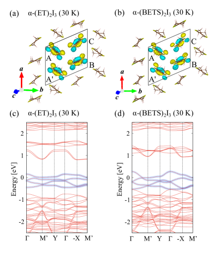
Figure 1: (Color online) Crystal structures and real-space distribution of MLWFs for (a) $\alpha$-(ET)₂I₃ and (b) $\alpha$-(BETS)₂I₃ at 30 K drawn by VESTA K. Momma and F. Izumi (2011). Four ET(BETS) molecules (labeled by A, A^′, B, and C sites) exist in the unit cell indicated by the black lines. The A and A^′ are crystallographically equivalent. Energy band structures for (c) $\alpha$-(ET)₂I₃ and (d) $\alpha$-(BETS)₂I₃ at 30 K. The solid lines are obtained by the DFT calculations, while the squares are obtained from the MLFWs. Here, we define $\Gamma\equiv(0,0,0)$, M’ $\equiv(-\pi,\pi,0)$, Y$\equiv(0,\pi,0)$, X $\equiv(\pi,0,0)$. The bandwidth for the four bands of $\alpha$-(ET)₂I₃ is approximately $3/4$ times smaller than that of $\alpha$-(BETS)₂I₃.

Using the MLWFs, we evaluate the transfer integrals for these compounds and the screened Coulomb interactions using the constrained random phase approximation (cRPA). The cutoff energy for the dielectric function is set at 5.0 Ry. The obtained effective Hamiltonian is given by

$$H=\sum_{{\bm{R}},{\bm{\delta}}}\sum_{\alpha,\beta,\sigma}(t^{(\bm{\delta})}_{(\alpha,\beta)}c^{{\dagger}}_{{\bm{R}},{\alpha},{\sigma}}c_{{\bm{R}}+{\bm{\delta}},\beta,{\sigma}}+{\rm H.c.})$$

$$+\sum_{{\bm{R}},\alpha}U_{\alpha}n_{{\bm{R}},\alpha,\uparrow}n_{{\bm{R}},\alpha,\downarrow}+\sum_{{\bm{R}},{\bm{\delta}}}\sum_{\alpha,\beta}V^{({\bm{\delta}})}_{(\alpha,\beta)}N_{{\bm{R}},\alpha}N_{{\bm{R}}+{\bm{\delta}},\beta}$$

where ${\bm{R}}$ denotes the unit cell coordinate, and the orbital and spin indices are indicated by $\alpha$, $\beta$ (A, A’, B, C) and $\sigma$ (+1: $\uparrow$, -1:$\downarrow$), respectively. The transfer integrals from $(\beta,\sigma)$ to $(\alpha,\sigma)$ separated by ${\bm{\delta}}$ are represented by $t^{({\bm{\delta}})}_{(\alpha,\beta)}$. The creation and annihilation operators are denoted by $c^{{\dagger}}_{{\bm{R}},{\alpha},{\sigma_{1}}}$ and $c_{{\bm{R}},{\alpha},{\sigma_{1}}}$, respectively. The number operators are defined as $n_{{\bm{R}},\alpha,\sigma}=c^{{\dagger}}_{{\bm{R}},{\alpha},{\sigma}}c_{{\bm{R}},{\alpha},{\sigma}}$ and $N_{{\bm{R}},\alpha}=n_{{\bm{R}},\alpha,\uparrow}+n_{{\bm{R}},\alpha,\downarrow}$. To reflect the two dimensionality of the effective Hamiltonians, we subtract a constant value $\Delta_{\rm DDF}$ from the on-site and off-site Coulomb interactions. Following a previous study, we take $\Delta_{\rm DDF}=0.20$eV for both compounds Nakamura et al. (2012). We confirm that the value of the constant shift does not change the result significantly.

Figure 2 shows schematic diagrams of the 2D conduction plane of (a) $\alpha$-(ET)₂I₃ and (b) $\alpha$-(BETS)₂I₃, showing the networks of transfer integrals and Coulomb interactions between the nearest-neighbor sites. We provide the values of the transfer integrals and the Coulomb interactions in the Supplemental materials sup and the raw data in the repository dat . In both materials, the $b$-axis direction transfer integrals $t_{b1}$ and $t_{b2}$ are approximately 10 times larger than the others and make a strong transfer chain along the $b$-axis direction. We note that in $\alpha$-(BETS)₂I₃, the strength of the transfer integral for $b1$ bond (A^′-C, $t_{b1}=138.1$ meV) is comparable to that for $b2$ bond (A^′-B, $t_{b2}=158.7$ meV). This indicates that the magnetic interactions between the A-A^′ chain and the B-C chain are frustrated. This geometrical frustration induces a dimensional reduction in the spin correlations as we show later. We can also see that the Coulomb interactions in $\alpha$-(ET)₂I₃ are around $1.25$ times larger than those in $\alpha$-(BETS)₂I₃.

mVMC analysis—To investigate the ground states of the effective Hamiltonians, we use the many-variable variational Monte Carlo (mVMC) method T. Misawa, S. Morita, K. Yoshimi et al. (2019). The trial wave function used in this study is given by

$$|\psi\rangle=\mathcal{P}_{G}\mathcal{P}_{J}\mathcal{L}_{S}|\phi_{\rm pair}\rangle,$$ (1)

where $\mathcal{L}_{S}$ represents the total spin projector and we use the spin singlet projection for the ground states. The Gutzwiller factor $\mathcal{P}_{G}$ and the Jastrow factor $\mathcal{P}_{J}$ are defined by

$$\mathcal{P}_{G}=\exp\Big{[}\sum_{i}g_{i}n_{i,\uparrow}n_{i,\downarrow}\Big{]},$$ (2)

$$\mathcal{P}_{J}=\exp\Big{[}\frac{1}{2}\sum_{i\neq j}v_{ij}N_{i}N_{j}\Big{]},$$ (3)

where we denote the combination of the unit cell coordinate and the orbital index as $i=(\bm{R},\alpha)$. The pair product part of the wave function $|\phi_{\rm pair}\rangle$ is defined as

$$|\phi_{\rm pair}\rangle=\left[\sum_{i,j}^{N_{\rm site}}f_{ij}c^{\dagger}_{i,\uparrow}c^{\dagger}_{j,\downarrow}\right]^{N_{\rm e}/2}|0\rangle,$$ (4)

where $N_{\rm site}$ and $N_{\rm e}$ represent the total number of sites and electrons, respectively. All variational parameters in the wavefunction are simultaneously optimized using the stochastic reconfiguration method S. Sorella (2001). We perform calculations for $L=4,6,8,10,12$ ($N_{\rm site}=4\times L^{2}$) with periodic boundary conditions. In the actual calculations, we impose a 2$\times$2 sublattice structure for the variational parameters. We take hopping parameters up to $\bm{R}=(\pm 2,\pm 2)$ and Coulomb interactions up to the nearest-neighbor bonds shown in Fig. 2(a). We also employ a particle–hole transformation to reduce the numerical cost.

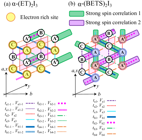
Figure 2: (Color online) Schematic diagrams of $\alpha$-type organic conductors for (a) $\alpha$-(ET)₂I₃ and (b) $\alpha$-(BETS)₂I₃ at 30K. Transfer integrals and Coulomb interactions for the nearest-neighbor sites are also shown. The shaded pink parallelogram shows a unit cell. We also show schematic picture of the ground state obtained by mVMC for (a) $\alpha$-(ET)₂I₃: horizontal stripe charge order (HCO) with spin dimer on strong transfer $t_{b2}$, and (b) $\alpha$-(BETS)₂I₃: one-dimensional antiferromagnetism (AF) correlations develop in A–A^′ chain. Molecules surrounded by shaded purple and green rectangles indicate bonds with a strong spin singlet correlation, and molecules with a shaded yellow circle are electron-rich sites.

Figures 2(a) and 2(b) also show the schematic charge configurations and spin correlations in real space for the ground states for $\alpha$-(ET)₂I₃ and $\alpha$-(BETS)₂I₃. In $\alpha$-(ET)₂I₃, the HCO insulator state is the ground state. The electron densities for $L=12$ at each site are $\langle n_{\rm A}\rangle=1.58$, $\langle n_{\rm{A}^{\prime}}\rangle=1.44$, $\langle n_{\rm B}\rangle=1.47$, and $\langle n_{\rm C}\rangle=1.51$. Statistical errors in Monte Carlo sampling for the electron densities are on the order of $10^{-4}$. We confirm that the system size dependence of local physical quantities such as electron density and spin correlation is small and, thus, in the following we show the result for $L=12$. In the HCO state, the spin correlation for the $b2{\rm-}1$ bond becomes large $\langle{\bm{S}}_{\rm{A}^{\prime}}\cdot{\bm{S}}_{\rm{B}}\rangle_{{b2{\rm-}1}}=-0.148(3)$, while the spin correlation for the $b3{\rm-}2$ bond becomes small, $\langle{\bm{S}}_{\rm B}\cdot{\bm{S}}_{\rm{A}^{\prime}}\rangle_{{b3{\rm-}2}}=-0.016(1)$. The parentheses denote the error–bars in the last digit. Because of the HCO, ths spin correlations between charge rich sites become small. For example, although the transfer integral of $b1{\rm-}1$ is comparable to that of $b2{\rm-}1$ ($t_{b1{\rm-}1}=97.48$meV and $t_{b2{\rm-}1}=136.2$meV), the spin correlation of $b1{\rm-}1$ bond is suppressed as $\langle{\bm{S}}_{\rm{A}}\cdot{\bm{S}}_{\rm{C}}\rangle_{{b1{\rm-}1}}=-0.034(1)$. These results indicate that the singlet dimer state associated with the emergence of HCO appears for the $b2{\rm-}1$ bond as shown in Fig. 2(a), which is consistent with the results of the NMR experiment and a previous theoretical study K. Ishikawa, M. Hirata, D. Liu, K. Miyagawa, M. Tamura, and K. Kanoda (2016); Y. Tanaka and M. Ogata (2016). By analyzing the effective Hamiltonians for the 150 K structure, we find that the Coulomb interactions induce instability toward the HCO state, although lattice distortion is important for stabilizing the HCO state. Details are shown in S.2 in Ref. [sup, ].

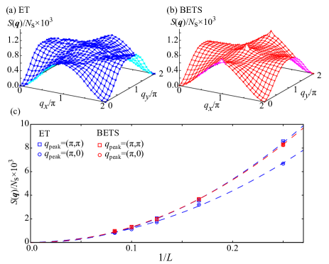
Figure 3: (Color online) Spin structure factors for (a)$\alpha$-(ET)₂I₃ and (b)$\alpha$-(BETS)₂I₃. We map the lattice structures into $2L\times 2L$ square lattices. The superposition of the $(\pi,0)$ and $(\pi,\pi)$ spin structures is consistent with the schematic images in Fig. 2. (c) System size dependence of peak values of spin structure factors. The broken curves show the results of fitting using the function $a(1/L)+b(1/L)^{2}$.

Figure 4: (Color online) Doping dependence of chemical potential for (a)$\alpha$-(ET)₂I₃ and (b)$\alpha$-(BETS)₂I₃, where $\mu_{0}=[\mu(N_{0}+1)-\mu(N_{0}-1)]/2$ and $N_{0}/N_{\rm s}=1.5$. For $\alpha$-(ET)₂I₃ and $\alpha$-(BETS)₂I₃, the estimated charge gap is $\Delta_{\rm c}\sim 0.1$eV and $\Delta_{\rm c}\sim 0.07$eV. For comparison, we plot the chemical potential for non-interacting systems for $L=12$ (brown crosses). (c) Size dependence of the spin gap. We fit the data for $L\geq 8$ using the linear function $a+b(1/L)$ to reduce the finite-size effects.

For $\alpha$-(BETS)₂I₃, we cannot find any clear signature of the charge ordering. The electron densities at each site are given by $\langle n_{\rm A}\rangle=1.49$, $\langle n_{\rm A^{\prime}}\rangle=1.49$, $\langle n_{\rm B}\rangle=1.50$, and $\langle n_{\rm C}\rangle=1.52$. Statistical errors in the Monte Carlo sampling are in order of $10^{-4}$. $n_{\rm A}=n_{\rm A^{\prime}}$ indicates that inversion symmetry is not broken. We find that the spin correlations become strong for the $a2$, $b1$, and $b2$ bonds. The spin correlations for these bonds are given by $\langle{\bm{S}}_{\rm A}\cdot{\bm{S}}_{\rm A^{\prime}}\rangle_{a3}=-0.0694(3)$, $\langle{\bm{S}}_{\rm A^{\prime}}\cdot{\bm{S}}_{\rm C}\rangle_{b1}=-0.0735(6)$, and $\langle{\bm{S}}_{\rm A^{\prime}}\cdot{\bm{S}}_{\rm B}\rangle_{b2}=-0.087(2)$. These antiferromagnetic spin correlations are schematically shown in Fig. 2(b). This result indicates that the magnetic interactions between A–A^′ and B–C chains are frustrated. Because of the inter-chain frustration, long-range antiferromagnetic order is absent in $\alpha$-(BETS)₂I₃.

Figures 3(a) and (b) show the spin structure factors defined as

$$S(\bm{q})=\frac{1}{N_{\rm s}}\sum_{i,j}\langle\bm{S}_{i}\cdot\bm{S}_{j}\rangle e^{i\bm{q}(\bm{r}_{i}-\bm{r}_{j})},$$ (5)

where we map the lattice structures to the $2L\times 2L$ square lattice (the directions of the $x$ and $y$ axes are shown in Fig. 2). In the actual calculation, we limit the summation of one index to within the unit cell to reduce the numerical cost. For $\alpha$-(ET)₂I₃, we find no significant peaks in the spin structure factors. This broad spin structure factor is consistent with the one-dimensional spin dimer structures in the A^′–B chain, as shown in Fig. 2(a).

We find that peaks appear at $\bm{q}=(\pi,0)$ and $(\pi,\pi)$ in $\alpha$-(BETS)₂I₃. The superposition of the $(\pi,0)$ and $(\pi,\pi)$ order indicates the emergence of the antiferromagnetic chain in the A–A^′ chain. Thus, the spin structure factor is consistent with the real space configuration in Fig. 2(b). However, the peak values become zero in the thermodynamic limit, as shown in Fig. 3(c). This result indicates that the one-dimensionality of the spin correlations prohibits long-range magnetic order even at zero temperature. Nevertheless, as we show below, the charge gap is finite due to the one-dimensional spin correlations.

Here, we discuss the charge and spin gap in $\alpha$-(ET)₂I₃ and $\alpha$-(BETS)₂I₃. In Figs. 4(a) and (b), we plot the chemical potential $\mu(N+1)=[E(N+2)-E(N)]/2$ ($E(N)$ is the total energy for $N$-electrons systems) as a function of the doping rate $\delta=N/N_{\rm s}-1.5$. From this plot, we estimate the charge gap to be $\Delta_{\rm c}\sim 0.1$eV ($\Delta_{\rm c}\sim 0.07$eV) for $\alpha$-(ET)₂I₃ ($\alpha$-(BETS)₂I₃). The amplitude of the charge gap in $\alpha$-(ET)₂I₃ is consistent with the experimental charge gap ($\Delta_{\rm c}\sim 0.07$eV) estimated from the optical conductivity Clauss et al. (2010). In $\alpha$-(ET)₂I₃, the existence of the charge gap is natural since the HCO and associated inversion symmetry breaking can open a gap for the massless Dirac electrons. However, the charge gap in $\alpha$-(BETS)₂I₃ cannot be explained by simple symmetry breaking since there is no clear signature of spin and charge ordering. This result indicates that the one-dimensional antiferromagnetic correlations developed in the A–A^′ bonds induce the gap for massless Dirac electrons. We note that the amplitude of the charge gap is sufficiently larger than that of the finite-size gap, which is about 0.01 eV. This indicates that the finite charge gap obtained by the mVMC calculations is not an artifact due to the finite system size.

Figure 4(c) shows the size dependence of the spin gap, defined as $\Delta_{\rm s}=E(S=1)-E(S=0)$. Using the spin quantum number projection, we obtain the energy of the triplet $(S=1)$ excited state. Although the size dependence is not smooth, it is likely that the spin gap is finite in the thermodynamic limit for $\alpha$-(ET)₂I₃. This is consistent with the existence of a spin dimer chain in A^′–B bonds. The amplitude of the spin gap, $\Delta_{\rm s}\sim 0.05$eV, is also consistent with the experimental result K. Ishikawa, M. Hirata, D. Liu, K. Miyagawa, M. Tamura, and K. Kanoda (2016). For $\alpha$-(BETS)₂I₃, the spin gap monotonically decreases except for $L=6$. A size extrapolation using data for $L\geq 8$ indicates that the spin gap almost vanishes in the thermodynamic limit. From the present calculation, although it is difficult to accurately estimate the spin gap in the thermodynamic limit, it is reasonable to conclude that the spin gap in $\alpha$-(BETS)₂I₃ is significantly smaller than that in $\alpha$-(ET)₂I₃.

Summary and Discussion—In this study, to determine the origin of gap opening for massless Dirac electrons in $\alpha$-(ET)₂I₃ and $\alpha$-(BETS)₂I₃, we derive the low-energy effective Hamiltonians and solve them using the mVMC method T. Misawa, S. Morita, K. Yoshimi et al. (2019). We find that the HCO insulator state appears in $\alpha$-(ET)₂I₃ while no clear symmetry breaking occurs in $\alpha$-(BETS)₂I₃. Nevertheless, we find that a charge gap opens in $\alpha$-(BETS)₂I₃ due to the development of one-dimensional spin correlations in the A–A^′ chain. We note that the recent observed increase in $1/(T_{1}T)$ of NMR below 20 K is consistent with the development of the one-dimensional spin correlations S. Fujiyama, H. Maebashi, N. Tajima, T. Tsumuraya, H-B. Cui, M. Ogata, and R. Kato (2022). We also note that weak but finite three dimensionality, which is not included in this study, can induce long-range magnetic order at low temperatures since the one-dimensional spin correlations are already developed in the conducting layer. Thus, the recently discovered antiferromagnetic order at low temperatures is consistent with our results T. Konoike, T. Terashima, S. Uji, Y. Hattori, and R. Kato (2022). Lastly, we consider the effects of spin–orbit coupling. Although spin–orbit coupling alone cannot explain the amplitude of the charge gap in $\alpha$-(BETS)₂I₃, the combination of the Coulomb interactions and spin–orbit coupling is intriguing since it can enhance the SOC effectively and stabilize the quantum spin Hall insulating phase S. Raghu, X. L. Qi, C. Honerkamp, and S. C. Zhang (2008); D. Ohki, K. Yoshimi, and A. Kobayashi (2022) or the three-dimensional topological insulator Nomoto et al. . To examine such effects, it is necessary to derive and solve $ab$ $initio$ Hamiltonians with spin–orbit coupling. This is an intriguing challenging issue but is left for future studies.

Supplemental Materials for “Gap opening mechanism for correlated Dirac electrons in organic compounds $\alpha$-(BEDT-TTF)₂I₃ and $\alpha$-(BEDT-TSeF)₂I₃”

I S.1. Details of microscopic parameters in $ab$ $initio$ Hamiltonians

Table 1 presents the transfer integrals and Coulomb interactions for $\alpha$-(ET)₂I₃ at 150 K and $\alpha$-(BETS)₂I₃ at 30 K, which have inversion symmetry, as shown in Fig. 5 (a). Table. 2 presents those for $\alpha$-(BETS)₂I₃ at 30 K. For $\alpha$-(ET)₂I₃ at 30 K, inversion symmetry is broken due to charge ordering. Thus, the relations of the bonds are more complicated, as shown in Fig.5 (b).

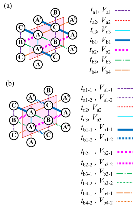
Figure 5: (Color online) (a) Schematic of lattice structure with inversion symmetry for $\alpha$-(ET)₂I₃ at 150 K and $\alpha$-(BETS)₂I₃ at 30 K. (b) Schematic of lattice structure without inversion symmetry for $\alpha$-(ET)₂I₃ at 30 K. The transfer integrals and Coulomb interactions for the nearest-neighbor sites are also shown. The pink shaded parallelogram shows a unit cell.

Table 1: List of transfer integrals $t$, difference in chemical potentials $\delta\mu_{\rm iC}\equiv\mu_{\rm i}-\mu_{\rm C}$ (i=A, A^′, and B), and effective Coulomb interactions $U$ and $V$ (units of meV) for $\alpha$-(ET)₂I₃ at 150 K and $\alpha$-(BETS)₂I₃ at 30 K. The values of $t$ and $V$ were averaged between the corresponding bonds shown in Fig. 5(a).

parameters	$\alpha$-(ET)2I3 (150 K)	$\alpha$-(BETS)2I3 (30 K)
$t_{\rm a1}$	$-$17.09	9.898
$t_{\rm a2}$	$-$36.10	$-$16.41
$t_{\rm a3}$	35.58	51.07
$t_{\rm b1}$	109.5	138.2
$t_{\rm b2}$	124.7	158.4
$t_{\rm b3}$	46.49	65.69
$t_{\rm b4}$	14.53	18.60
$\delta\mu_{\rm AC}$	3.15	$-$7.059
$\delta\mu_{\rm A^{\prime}C}$	2.48	$-$7.816
$\delta\mu_{\rm BC}$	5.28	$-$13.17
$U_{\rm A}$	1750	1389
$U_{\rm A^{\prime}}$	1750	1389
$U_{\rm B}$	1772	1405
$U_{\rm C}$	1738	1358
$V_{\rm a1}$	662.6	580.5
$V_{\rm a2}$	686.9	596.2
$V_{\rm a3}$	636.7	566.7
$V_{\rm b1}$	636.2	579.9
$V_{\rm b2}$	625.7	572.9
$V_{\rm b3}$	583.2	537.8
$V_{\rm b4}$	608.3	556.9

Table 2: List of transfer integrals $t$, difference im chemical potentials $\delta\mu_{\rm iC}\equiv\mu_{\rm i}-\mu_{\rm C}$ (i=A, A^′, and B), and effective Coulomb interactions $U$ and $V$ (units of meV) for $\alpha$-(ET)₂I₃ at 30 K. The corresponding bonds are shown in Fig. 5(b).

parameters	$\alpha$-(ET)2I3 (30 K)
$t_{\rm a1-1},t_{\rm a1-2}$	$-$30.12, $-$5.250
$t_{\rm a2}$	$-$37.51
$t_{\rm a3}$	38.07
$t_{\rm b1-1},t_{\rm b1-2}$	97.48, 124.6
$t_{\rm b2-1},t_{\rm b2-2}$	136.2, 125.5
$t_{\rm b3-1},t_{\rm b3-2}$	44.92, 44.96
$t_{\rm b4-1},t_{\rm b4-2}$	24.17, 1.806
$\delta\mu_{\rm AC}$	1.111
$\delta\mu_{\rm A^{\prime}C}$	12.87
$\delta\mu_{\rm BC}$	22.44
$U_{\rm A}$	1735
$U_{\rm A^{\prime}}$	1732
$U_{\rm B}$	1763
$U_{\rm C}$	1722
$V_{\rm a1-1},V_{\rm a1-2}$	650.1, 652.9
$V_{\rm a2}$	676.5
$V_{\rm a3}$	626.6
$V_{\rm b1-1},V_{\rm b1-2}$	612.8, 634.4
$V_{\rm b2-1},V_{\rm b2-2}$	618.5, 613.1
$V_{\rm b3-1},V_{\rm b3-2}$	577.5, 564.2
$V_{\rm b4-1},V_{\rm b4-2}$	606.6, 591.4

II S.2. Stability of charge-ordered state in $\alpha$-(ET)₂I₃ at 150K

We solve the effective Hamiltonians for $\alpha$-(ET)₂I₃ with 150 K structures using mVMC. The forms of the wavefunctions for mVMC are the same as those explained in the main text. In the Hamiltonian for the 150 K structure, since the inversion symmetry is not broken, the chemical potentials for the A and A^′ sites are equivalent within the order of meV. For this Hamiltonian, we obtain two different states, the horizontal stripe charge ordered (HCO) state and non-HCO state for $L\geq 8$. For $L=12$, the charge densities for the HCO state are given by $\langle n_{\rm A}\rangle=1.47$, $\langle n_{\rm A^{\prime}}\rangle=1.49$, $\langle n_{\rm B}\rangle=1.52$, and $\langle n_{\rm C}\rangle=1.51$ and the charge densities for the non-HCO state are $\langle n_{\rm A}\rangle=1.48$, $\langle n_{\rm A^{\prime}}\rangle=1.48$, $\langle n_{\rm B}\rangle=1.52$, and $\langle n_{\rm C}\rangle=1.51$. The statistical errors in the Monte Carlo sampling for the electron densities are of the order of $10^{-3}$. We confirm that the size dependence of the charge densities is negligibly small. The difference in the charge densities for the A and A^′ sites is about 0.02, and is smaller than that obtained for the Hamiltonians with a 30 K structure ($\sim 0.06$). We also find that the HCO and non-HCO states are almost degenerate and their energy difference is below 1 meV, as shown in Fig. 6. This result indicates that the lattice distortion also plays an important role in stabilizing the HCO states although the Coulomb interactions alone induce instability toward the HCO state.

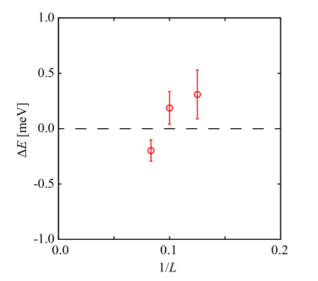
Figure 6: (Color online) Energy difference between HCO and non-HCO states defined as $\Delta E=E_{\rm HCO}/N_{\rm s}-E_{\rm non-HCT}/N_{\rm s}$.