Is LTT 1445 Ab a Hycean World or a cold Haber World? Exploring the Potential of Twinkle to Unveil Its Nature

Abstract

We explore the prospects for Twinkle to determine the atmospheric composition of the nearby terrestrial-like planet LTT 1445 Ab, including the possibility of detecting the potential biosignature ammonia (NH₃). At a distance of 6.9 pc, this system is the second closest known transiting system and will be observed through transmission spectroscopy with the upcoming Twinkle mission. Twinkle is equipped with a 0.45 m telescope, covers a spectral wavelength range of 0.5 - 4.5 $\mu$m simultaneously with a resolving power between 50 - 70, and is designed to study exoplanets, bright stars, and solar system objects. We investigate the mission’s potential to study LTT 1445 Ab and find that Twinkle data can distinguish between a cold Haber World (N₂-H₂-dominated atmosphere) and a Hycean World with a H₂O-H₂-dominated atmosphere, with a $\chi_{\nu}^{2}$ = 3.01. Interior composition analysis favors a Haber World scenario for LTT 1445 Ab, which suggests that the planet probably lacks a substantial water layer. We use petitRADTRANS and a Twinkle simulator to simulate transmission spectra for the more likely scenario of a cold Haber World for which NH₃ is considered to be a biosignature. We study the detectability under different scenarios: varying hydrogen fraction, concentration of ammonia, and cloud coverage. We find that ammonia can be detected at a $\sim$ 3$\sigma$ level for optimal (non-cloudy) conditions with 25 transits and a volume mixing ration of 4.0 ppm of NH₃. We provide examples of retrieval analysis to constrain potential NH₃ and H₂O in the atmosphere. Our study illustrates the potential of Twinkle to characterize atmospheres of potentially habitable exoplanets.

1 Introduction

Twinkle is an upcoming space-based telescope with a 0.45 m primary aperture and a broad visible to infrared wavelength coverage (0.5 – 4.5 $\mu$m). The Twinkle space mission (Stotesbury et al., 2022) will conduct two simultaneous surveys during its first three years of operation, which is scheduled to begin in 2025. While one of these will focus on studying objects within our own solar system, the other will be dedicated to the study of extrasolar targets. A large portion of the latter survey will be used to study exoplanet atmospheres, the science case for which Twinkle was originally conceived (Edwards et al., 2019). There are nearly 900 confirmed transiting exoplanets within Twinkle’s field of view, as well as over 1400 planet candidates from the Transiting Exoplanet Survey Satellite (TESS, Ricker et al. 2015), offering the potential for a structured population survey of exoplanet atmospheres.

Twinkle can be highly complementary to the James Webb Space Telescope (JWST). While JWST will deliver unprecedentedly precise data, there will be limited time allocated to exoplanet sciences. Therefore, it is likely to only be used to observe the most exciting targets. To this end, Twinkle can provide low-resolution spectroscopy to provide an initial atmospheric characterization to promote further study or be used to refine planetary and orbital parameters. Moreover, certain JWST instruments/modes cannot observe bright targets due to saturation limits, and Twinkle can fill in the gap for bright targets. Furthermore, the planets studied with Twinkle can be methodically selected, building up large sets of data with specific goals in mind whereas each JWST proposal often focuses only on a small number of worlds. Combining Twinkle data with the JWST mission will allow us to achieve a more comprehensive picture of exoplanet atmospheres.

The Kepler Space Mission (Borucki et al., 2010) has shown that super-Earths/mini-Neptunes are amongst the most abundant type of planet (Fressin et al. 2013; Fulton et al. 2017). There is an observed gap in the distribution of these planet sizes, known as the radius valley (Fulton et al. 2017; Van Eylen et al. 2018). Below the radius valley ($<$ 1.5 R_⊕), these planets are known as super-Earths/terrestrial-like planets. Studies have investigated their ability to hold onto a hydrogen-based atmosphere due to their decreased mass and decreased surface gravity from both ground-based (Diamond-Lowe et al. 2018; Diamond-Lowe et al. 2020) and space-based observatories (Edwards et al., 2021).

Planets with H₂/He dominated atmospheres may be more amenable targets for transmission spectroscopy with upcoming space-based missions such as Twinkle. The presence of H₂ can raise the scale height and therefore the transmission signal features for observations (Miller-Ricci et al. 2008; Hu et al. 2021). H₂-dominated atmospheres may also produce different biosignatures, such as NH₃ in cold Haber Worlds (Seager et al., 2013a).

In this work we assess the detectability of the potential biosignature ammonia on the terrestrial-like planet, LTT 1445 Ab with the upcoming Twinkle space mission. We first provide a summary of previous literature on ammonia as a potential biosignature in §2. We then describe the target selection process for the study in §3. The process to distinguish LTT 1445 Ab from a cold Haber World or Hycean World is described in §4. Major findings on the detectability of NH₃ are presented in §5. Finally, we present our retrieval analysis to support the major findings in §6 and conclude in §7.

2 Ammonia as a Potential Biosignature

Seager et al. (2013a) first proposed NH₃ as a biosignature gas in a H₂ and N₂ dominated atmosphere – nicknamed a cold Haber World (e.g. Seager et al. 2013b; Huang et al. 2021). Cold Haber Worlds are named after the Haber-Bosch process which is the main industrial process for producing NH₃ from N₂ from the air, H₂ and an iron catalyst, combined with high temperatures and pressures. The reaction is as follows:

$$3H_{2}+N_{2}\longrightarrow 2NH_{3}$$

Since the proposal of NH₃ as a biosignature, there have been a multitude of studies to investigate its detectability with JWST and future Extremely Large Telescopes (e.g. Chouqar et al. 2020; Wunderlich et al. 2020; Phillips et al. 2021; Ranjan et al. 2022). Phillips et al. (2021) explored the detection of the potential biosignature NH₃ in gas dwarfs, exoplanets with radii between Earth and Neptune with potentially H₂ dominated atmospheres. They found that a minimum of 0.4 ppm would be needed to detect the ammonia features in transmission spectroscopy with the NIRSpec and NIRISS (SOSS) instruments/modes on JWST, given optimal cloud-free atmospheric conditions. Huang et al. (2021) assessed ammonia as a potential biosignature in terrestrial-like planets and found that a minimum of 5.0 ppm ammonia in the atmosphere would be needed to be detectable by JWST using the NIRSpec/G395M mode for the 3.0 $\mu$m ammonia feature.

Although NH₃ is a strong candidate biosignature in H₂ and N₂ atmospheres, there is still need to consider the potential of false positives. An overview of false positives of NH₃ was provided by Seager et al. 2013b and Catling et al. 2018, alongside thesis work by Evan Sneed. Recently, Huang et al. (2021) laid out a few examples of minor abiotic sources of NH₃ for Earth/terrestrial-like planets including: trace components in volcanic gas eruptions, iron doping TiO₂ containing sands, and lightning.

3 Target Selection

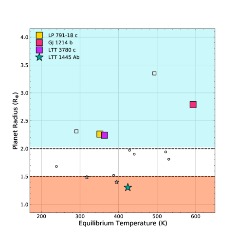
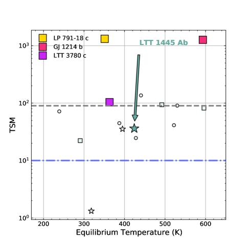
Figure 1: Left: Planet radius (R${}_{\oplus})$ vs equilibrium temperature (K) for Twinkle objects that meet initial selection criteria (1-3). The orange shaded region and star shapes are objects below the radius valley (<1.7 R_⊕). Objects within the radius valley (1.5 – 2.0 R_⊕) are marked with circle shapes. The blue shaded regions and square markers are targets above the radius valley (>2.0 R_⊕). The target of interest for this study LTT 1445 Ab is marked with a blue-green star. Right: The modified transmission spectroscopy metric (TSM) for H-band defined by Kempton et al. (2018). There are larger planets above the radius valley with the highest TSM: GJ 1214 b (pink square), LTT 3780 c (purple square), and LP 791-18 c (gold square). However, these targets have low S/N estimates with Twinkle for 25 transits. The horizontal grey line represents the recommended TSM threshold for targets (R = 1.5 – 10.0 $R_{\oplus}$) to be considered to be selected for high quality atmospheric characterization (Kempton et al., 2018). The purple dotted-dashed line represents the threshold TSM values (TSM $>$ 10) for terrestrial like planets ($<$1.5 R_⊕).

We explore possible targets of interest for characterization that are within the field of view for Twinkle. Targets are evaluated using the following criteria: (1) planet radii between 1.3 and 3.4 R_⊕, (2) equilibrium temperature (T_eq) below 650 K, (3) distance within 50 pc, (4) an initial S/N estimation (<S/N> $\geq$ 3$\sigma$) for Twinkle using TwinkleRad (Edwards & Stotesbury, 2021) for a baseline of 25 transits and (5) a modified transmission spectroscopy metric (TSM) from Kempton et al. (2018) (see Equation 1).

Compared to the work in Phillips et al. (2021), we use an expanded parameter space of radii and equilibrium temperatures. Nixon & Madhusudhan (2021) found that the phase structure of water-rich sub-Neptunes show indication that planets with a H/He envelope could host liquid H₂O in the liquid phase at up to 647 K at pressures of $218$ to $7\times$10⁴ bar. We also explore a slightly lower radius space (1.3 R_⊕), as Huang et al. (2021) evaluated ammonia as a promising biosignature on terrestrial-like planets (e.g. a 1.75 R_⊕, and 10 M_⊕ exoplanet around an M-dwarf).

We search the NASA Exoplanet Archive for targets that meet our criteria. We find that LTT 1445 Ab has the highest (modified) TSM for terrestrial targets below the radius valley (Figure 1). We also explore targets that lie within the radius valley, but find low S/N estimates for NH₃ detection given the baseline of 25 transits. Initially objects such as GJ 1214 b, LP 791-18 c, and LTT 3780 c meet the first three criteria for target selection and produce high TSM metrics for planets above the radius valley. However, these targets either have known flat transmission spectra (Kreidberg et al., 2014) and/or currently have low S/N estimates for Twinkle. We therefore focus on LTT 1445 Ab in subsequent analyses.

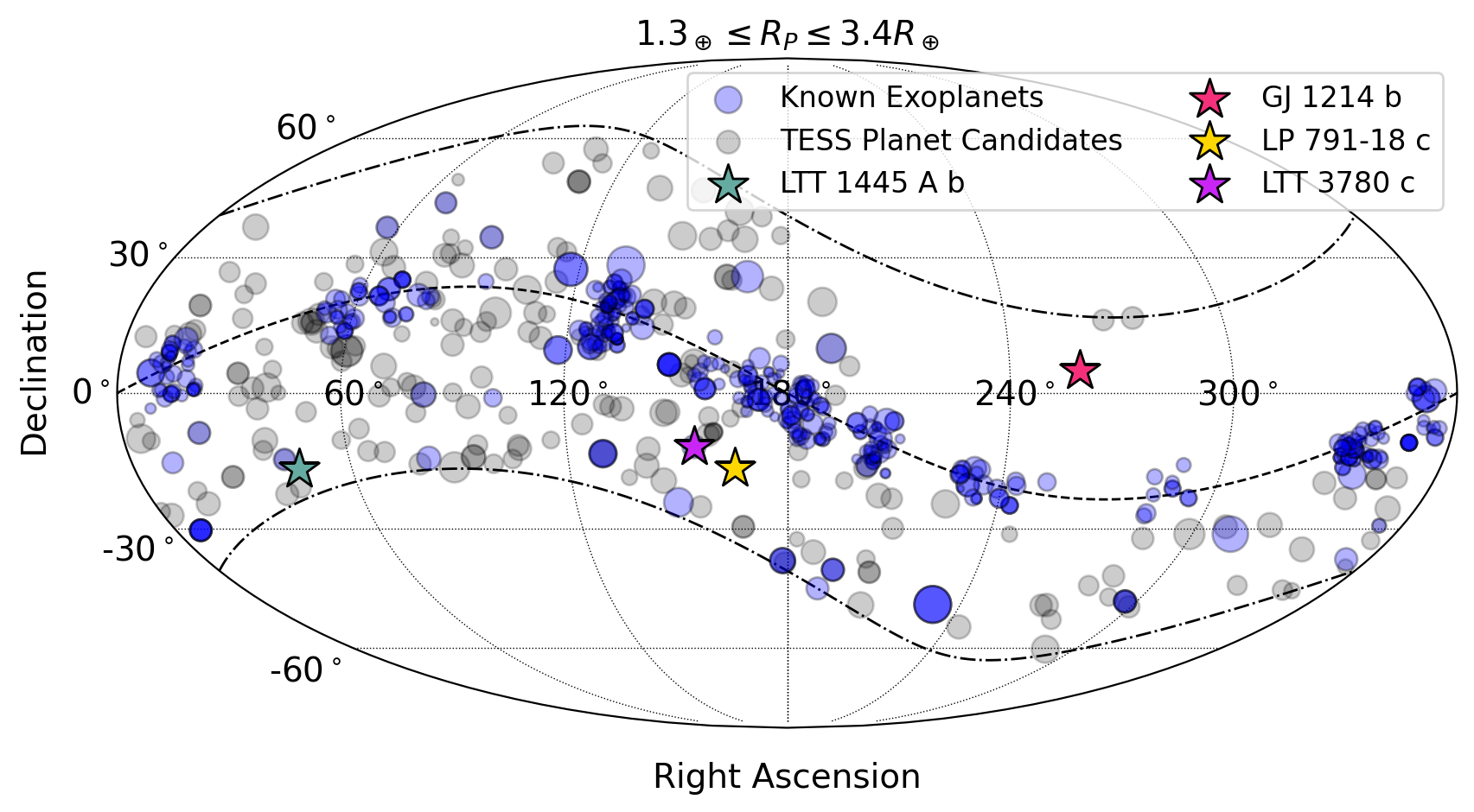
Figure 2: Field of view showing known exoplanets (blue circles) with planetary size (1.3_⊕ $\leq$ R_p $\leq$ 3.4_⊕ ). The $TESS$ planet candidates are shown in the gray markers. The size of the markers correspond to the host star’s K-band magnitude. The target of interest for this paper LTT 1445 Ab is shown with a star marker. GJ 1214 b, LP 791-18 c, LTT 3780 c are shown with a pink, gold, and purple star respectively.

3.1 LTT 1445 Ab

Since LTT 1445 Ab is a potential target, we provide a brief introduction of the system. LTT 1445 Ab lies at a distance of 0.038 AU from its host star and has an orbital period of 5.4 days (Winters et al., 2019). The host system is comprised of three mid-to-late M dwarfs. The host star, LTT 1445 A, is bright (K_s = 6.50 mag). LTT 1445 A is also the closest M-dwarf to host a transiting planet (Winters et al., 2021), making this system a prime target for atmospheric characterization. A summary of key stellar and planetary parameters is shown in Table 1. During the first three years of operations, Twinkle will conduct an extrasolar survey (Stotesbury et al., 2022). We use the tool from Edwards & Stotesbury (2021) to determine that, during the time frame of this survey, there will be 29 transits available for observation with Twinkle.

Table 1: Planetary and stellar parameters for LTT 1445 Ab from Winters et al. 2021

Mp (M⊕)	2.87${}^{+0.26}_{-0.25}$
Rp (R⊕)	1.304${}^{+0.067}_{-0.060}$
Teq(K)	424$\pm$21
Distance (pc)	14.98$\pm$0.01
H-bands (mag)	6.774$\pm$0.038
Ts (K)	3337$\pm$150
logg (dex)	3.217${}^{+0.050}_{-0.053}$
t14(hrs)	1.367${}^{+0.017}_{-0.016}$
Fe/H (dex)	-0.34$\pm$0.08
Eccentricity	0.19${}^{+0.35}_{-0.14}$

Despite the relative small size of LTT 1445 Ab, it is a target of interest for atmospheric studies. Winters et al. (2021) calculate a TSM of 30 for LTT 1445 Ab which is higher than those for LHS 1140 b (Dittmann et al., 2017) and TRAPPIST 1-f (Gillon et al., 2017). We implement a modified version of the Kempton TSM (Equation 1),

$$\rm{TSM}=(\rm{Scale\ factor})\times\frac{R_{p}^{3}T_{eq}}{M_{p}R_{\star}^{2}}\times 10^{-m_{x}/5}$$ (1)

In Equation 1, $T_{eq}$ is the planet equilibrium temperature in Kelvin, $R_{p}$ is the planet radius is Earth radii, $M_{p}$ is the planet mass in Earth mass, $R_{\star}$ is the host star radius in solar radii, and $m_{x}$ is the apparent magnitude of the host star.

The Scale factor in Equation 1 is designed to be a normalization constant to give near-realistic S/N values for 10 hr observing with the JWST/NIRISS instrument (Kempton et al., 2018). The scale factor is different for planets with R < 1.5 R_⊕ (scale factor = 0.190) and planets with 1.5 R_⊕ < R < 2.75 R_⊕ (scale factor = 1.26). For more details about the method used and scale factor determination, see Kempton et al. (2018).

We adopt the TSM equation for the Twinkle wavelength coverage of 0.4 – 4.5 $\mu$m coverage, for the H-band coverage and L-band coverage. The H-band region is approximately the central wavelength for Channel 0 for Twinkle which covers 0.5 - 2.4 microns. The L-band region is approximately the central wavelength for Channel 1 for Twinkle which covers 2.4 - 4.5 microns. We find a H-band TSM of 36.0 (Figure 1) and L-band TSM of 44.0.

4 A Haber World vs. A Hycean World

In this section we explore the scenario of LTT 1445 Ab as a Hycean world (Madhusudhan et al., 2021) and its implications for detection with Twinkle. A Hycean world is defined as a planet that has a water-rich interior with massive oceans underneath a H₂-dominated atmosphere (Madhusudhan et al., 2021) We also use the bulk properties (M_p and R_p) of LTT 1445 Ab to constrain the interior composition and to assist with distinguishing a cold Haber World from a Hycean World.

As shown in §4.2, our interior composition analysis indicates that LTT 1445 Ab is likely not a Hycean world. As a result, we model LTT 1445 Ab as a cold Haber World.

4.1 Simulating a cold Haber World Spectrum

We use the Python package, petitRADTRANS (Mollière et al., 2019), to simulate the planetary atmosphere for transmission spectroscopy. Similar to Phillips et al. (2021), we utilize the low resolution mode and use a 1-D Gaussian Kernel to smooth the spectra to the Twinkle Channel 0 (0.5 – 2.4 $\mu$m) and Channel 1 (2.4 – 4.5 $\mu$m) resolution of R = 70 and R = 50 respectively. The reference pressure is set to $P_{0}$ = 1.0 bar. We consider lower pressures in the atmosphere in this work, expanding from the lower bound of the P-T profile of Earth. We use lower pressure value of 10^-9 bar, opposed to a lower 10^-6 bar pressure from an adjusted P-T profile of Earth (Phillips et al., 2021).

We modeled the performance of Twinkle using TwinkleRad, an adapted version of the radiometric tool described in Mugnai et al. (2020). We note that, due to the ongoing detailed design work, there are currently significant performance margins built-in to this simulator.

We employ the same methods used in Phillips et al. (2021) to calculate the atmospheric composition for a cold Haber world. We use the the values in Table 2 to build the synthetic spectrum with a base atmosphere of 90 per cent H₂ and 10 per cent N₂. A fixed number of 25 transits is set to determine NH₃ is detectable. TauREx 3 (Al-Refaie et al., 2021) is used to rebin the spectra. Synthetic noise is added using a random Gaussian distribution. The S/N detection metric and threshold (<S/N> $\geq$ 3$\sigma$) is the same as in Phillips et al. (2021). The simulation for 25 transits with Twinkle with the corresponding S/N is shown in Figure 3.

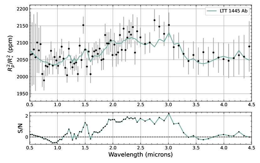
Figure 3: Top: Simulated cold Haber World transmission spectra of LTT 1445 Ab with 25 transits. Low mean molecular weight case ($\mu$ $\sim$ 4.5). Bottom: The corresponding S/N

Table 2: Species used for petitRADTRANS to generate synthetic spectra with 90 per cent H₂ and 10 per cent N₂ atmosphere for a cold Haber World. Notes: (a) We adopt the mixing ratios for gases other than N₂ or H₂ (Seager et al., 2013b), assuming no major change in the chemistry (b) N₂ has no rotational-vibrational transitions, so there are no signatures observable at infrared wavelengths, so this feature is not available in petitRADTRANS but is used to determine the mean molecular weight of the atmosphere

. Species VMR^a MMR H₂O 9.17$\times$10^-7 3.62$\times$10^-6 CO₂ 2.90$\times$10^-9 2.81$\times$10^-8 CH₄ 2.90$\times$10^-8 1.02$\times$10^-7 H₂ 8.25$\times$10^-1 3.62$\times$10^-1 CO 9.17$\times$10^-10 5.64$\times$10^-9 OH 9.17$\times$10^-16 3.42$\times$10^-15 HCN 9.17$\times$10^-10 5.44$\times$10^-9 NH₃ 3.6$\times$10^-6 1.37$\times$10^-5 N₂^b 9.17$\times$10^-2 5.64$\times$10^-1 He 8.25$\times$10^-2 7.25$\times$10^-2

4.2 Can Twinkle Distinguish a cold Haber World from a Hycean World?

While LTT 1445 Ab is not in the traditional habitable zone of its star (Winters et al., 2019), it is considered as a candidate Hycean world where a liquid ocean may exist underneath a H₂-dominated atmosphere. In a Hycean world scenario, LTT 1445 Ab lies in the Hycean habitable zone. The Hycean habitable zone is defined as regions corresponding to the maximum irradiation that allows for habitable conditions at the surface of the ocean (Madhusudhan et al., 2021). For a Hycean world, Madhusudhan et al. (2021) consider H₂O, CH₄, and NH₃ as potentially abundant molecules in a H₂-based atmosphere. The question remains if we can use Twinkle to distinguish between a Hycean world and a cold Haber world. This is an important question because detecting NH₃ needs to be put into larger context of which world it belongs to. For a cold Haber world, NH₃ is regarded as a biosignature (Seager et al. 2013a), however, NH₃ detection may be unrelated to life in a Hycean world but nonetheless is a critical chemical species in the atmosphere (Madhusudhan et al., 2021).

In order to distinguish between two worlds, we first simulate Twinkle observations of a Hycean world for LTT 1445 Ab. Then, we compare the simulated data with that of a cold Haber world using a reduced $\chi^{2}$ statistic. Below we detail the two steps.

We simulate the Hycean-case scenario for LTT 1445 Ab by adopting the volume mixing ratios provided in Madhusudhan et al. (2021). In their work, they assume a volume mixing ratio of 0.1, 5.0 $\times$10^-4, and 1.3 $\times$ 10^-4 for H₂O, CH₄, and NH₃ respectively. We then convert these values to mass mixing ratios (Table 3). We use these mass mixing ratios as input to petitRADTRANS and simulate the atmosphere. The pressure bar is set to P₀ = 1.0 bar, low resolution mode is used, and an 424 K isothermal atmosphere is assumed.

Table 3: Species used for petitRADTRANS to generate synthetic Hycean-world spectra atmosphere, adopted from Madhusudhan et al. (2021)

Species	VMR	MMR
H2O	7.26$\times$10-2	2.39$\times$10-1
CH4	2.90$\times$10-8	1.02$\times$10-7
H2	6.54$\times$10-1	2.39$\times$10-1
NH3	3.66$\times$10-6	1.37$\times$10-5

To quantify if a cold Haber world and Hycean world can be distinguished with Twinkle, we implement a $\chi^{2}$ statistical test (Equation 2), and sample the petitRADTRANS spectrum to a common wavelength grid. We then calculate the reduced $\chi^{2}$ statistic, $\chi_{\nu}^{2}\equiv\chi^{2}/\nu$, where $\nu$ represents the number of degrees of freedom.

$$\chi^{2}=\sum_{i=0}^{n-1}\frac{(Hycean_{i}-Haber_{i})^{2}}{\sigma_{i}^{2}}$$ (2)

In Equation 2, subscript $i$ is the wavelength index to match the Twinkle wavelength grid, Hycean indicates the spectrum for a Hycean World, Haber indicates the spectrum for a cold Haber world, and $\sigma$ is the expected noise for 25 transits observed by Twinkle. Based on this metric we find a $\chi_{\nu}^{2}=3.01$, indicating that Twinkle can distinguish between a cold Haber world and a Hycean world (Figure 4).

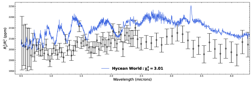
Figure 4: Simulated transmission spectra of LTT 1445 Ab as a cold Haber world with 90 per cent H₂ (black points with error bars) compared to a theoretical spectrum of a Hycean world (blue).

4.3 Composition of LTT 1445 Ab

With a planet mass and radius uncertainty of 9 per cent and 5 per cent (Winters et al., 2021), LTT 1445 Ab is among the best characterized small planets. Such precision in its mass and radius allows us to place constraints on its composition. In Figure 5, we show theoretical mass-radius composition curves (Zeng et al., 2019) and place LTT 1445 Ab in the context of other small exoplanets from the literature that are within Twinkle’s field of view. LTT 1445 Ab falls near the Earth-like composition curve of 67 per cent magnesium silicate and 33 per cent iron, suggesting that it is likely a rocky planet without a substantial water layer.

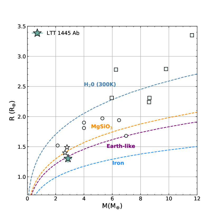
Figure 5: Mass-radius diagram for future targets of interest along with LTT 1445 Ab (blue star). The star markers correspond to objects below the radius valley (R < 1.5 $R_{\oplus}$). The circle markers correspond to objects within the radius valley (1.5 < $R_{\oplus}$ < 2.0). The square markers are those targets above the radius valley ($R_{\oplus}$ > 2.0). LTT 1445 Ab falls near the composition curve corresponding to an Earth-like planet. The curves are interior structure models of 100 per cent water (dark blue), 100 per cent magnesium silicate rock (orange), 33 per cent iron plus 67 per cent rock (purple) (i.e., Earth-like), and 100 percent iron (light blue). The values are from Zeng et al. 2019.

We further explore the interior composition of LTT 1445 Ab and calculate its core mass fraction (CMF) using the ExoPlex software (Unterborn et al., 2018; Schulze et al., 2020), which solves the equations of planetary structure and calculates a CMF for a given planet mass and radius. ExoPlex assumes a two-layer planet consisting of an iron core and a pure, magnesium silicate ($\rm MgSiO_{3}$) mantle. Assuming the planet mass and radius from Winters et al. (2021) of $R_{p}=1.304^{+0.067}_{-0.060}~{}R_{\oplus}$ and $M_{p}=2.87\pm 0.25~{}M_{\oplus}$, we obtain a CMF of $\rm CMF=0.42^{+0.18}_{-0.17}$. This value is consistent with the value of $\rm CMF=0.42\pm 0.28$ reported by Winters et al. (2021), calculated using the semi-empirical relations of Zeng & Jacobsen (2017). As an alternative check on the CMF, we calculated the core radius fraction (CRF) using HARDCORE (Suissa et al., 2018), and obtain a value of $\rm CRF=0.67\pm 0.14$, which can be easily converted to a CMF using the empirical relations from Zeng et al. (2016). From that, we obtain $\rm CMF=0.45\pm 0.08$, which is consistent with the value from Exoplex.

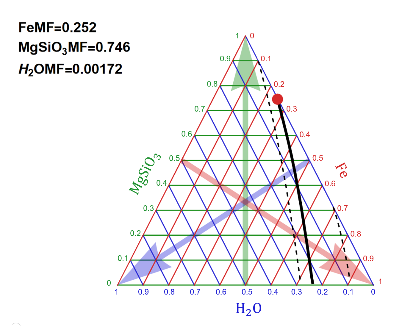
Figure 6: Ternary diagram showing the possible compositions of LTT 1445 Ab using the models from Zeng & Sasselov (2013). The red dot denotes relative mass fractions (MF) of the three layers (Fe, $\rm MgSiO_{3}$, $\rm H_{2}O$). The solid black line represents all the possible mass combinations of these layers allowed by the planet’s mass and radius, and the black dashed lines represent the uncertainties. The best-fit solution indicates that LTT 1445 Ab has a negligible fraction of water, likely ruling it out as a Hycean world.

We also investigated the interior composition of LTT 1445 Ab using the theoretical models of Zeng & Sasselov (2013). In these models, the planet consists of three layers: an iron core, a magnesium silicate mantle ($\rm MgSiO_{3}$), and a water layer overlaying the mantle and iron core. Figure 6 shows a ternary diagram with the range of compositions allowed within the uncertainties of the mass and radius of LTT 1445 Ab. We obtain an iron mass fraction of 0.252, a silicate mass fraction of 0.746, and a water mass fraction of 0.002. Some of the other possible solutions along the black line are disfavored for theoretical reasons. For example, a planet consisting purely of water and iron is physically unlikely ($\sim$25 per cent $\rm H_{2}O$ and $\sim$75 per cent Fe core), e.g., Marcus et al. (2010). The best-fit solution indicates that LTT 1445 Ab is likely a dry planet, i.e., not a Hycean world as proposed by Madhusudhan et al. (2021). According to Madhusudhan et al. 2021, a typical Hycean planet would have an H₂-rich atmosphere and a H₂O layer with a water mass fraction between 10 per cent and 90 per cent, and iron core + mantle with at least a 10 per cent mass fraction.

The discrepancy between the classification of Madhusudhan et al. (2021) and ours is probably due to the lower mass they used of $\sim$2.2 $M_{\oplus}$. The revised larger mass with lower uncertainty reported by Winters et al. (2021) leads to a higher density and a more Earth-like, rocky composition, thus ruling out the presence of a thick ocean layer.

5 Main Results on NH₃ Detection

5.1 What fraction of hydrogen is Twinkle sensitive to?

Small planets (R $\lessapprox$ 1.6 R_⊕) have less gravity and can be prone to losing their atmospheres. Atmospheric loss can be due to either core powered atmospheric mass loss (Gupta & Schlichting 2021 and references therein) and/or photoevaporation atmospheric mass loss (e.g. Lopez & Fortney 2013; Owen & Wu 2017; Ginzburg et al. 2018).

We explore the scenario of likely H₂ mass loss of LTT 1445 Ab and see which lower limit fraction of hydrogen Twinkle is sensitive to. We follow Chouqar et al. 2020 and Phillips et al. 2021 and consider the following scenarios: a hydrogen-rich atmosphere (90 per cent H₂ and 10 per cent N₂), a hydrogen-poor atmosphere (1 per cent H₂ and 99 per cent N₂) and a hydrogen-intermediate atmosphere (75 per cent H₂ and 25 per cent N₂)(Figure 7).

We determine the effects of a reduction in hydrogen in the atmosphere on the detection of ammonia. For LTT 1445 Ab we find that the atmosphere would need to be H-rich (90 per cent H₂) to be detectable by Twinkle (Table 4).

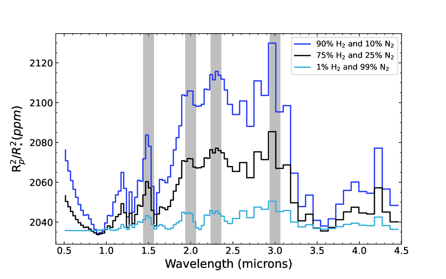
Figure 7: Modeled transmission spectra of LTT 1445 Ab showing various atmospheric compositions compositions. The lines represent different hydrogen dominated scenarios: a H-rich atmosphere (90 per cent H₂ and 10 per cent N₂), a H-poor atmosphere (1 per cent H₂ and 99 per cent N₂), and a H-intermediate atmosphere (75 per cent H₂ and 25 per cent N₂). Contributing NH₃ features are shown in grey.

Table 4: Average S/N of major NH₃ transmission features for LTT 1445 Ab transmission spectroscopy for different atmospheric compositions.

LTT 1445 Ab	Ammonia Feature	S/N	Total <S/N>
	[$\mu$m]	[$\sigma$]	[$\sigma$]
H-rich	1.5	1.13	3.10
	2.0	1.56
	2.3	1.75
	3.0	1.67
H-intermediate	1.5	0.69	1.79
	2.0	0.89
	2.3	0.99
	3.0	0.97
H-poor	1.5	0.61	1.08
	2.0	0.47
	2.3	0.49
	3.0	0.57

5.2 Other factors that impact NH₃ detection: ammonia concentration and clouds

The lifetime and concentration of NH₃ in a H₂ dominated atmosphere has been previously studied (e.g. Tsai et al. 2021; Ranjan et al. 2022). We explore how the concentration of ammonia affects the S/N detection in the atmosphere of LTT 1445 Ab.

Tsai et al. 2021 explored the evolution of the column mixing ratio for NH₃ for an atmosphere with 1-bar surface with a planet around a quiet M-dwarf host and a planet around an active M-dwarf host. They found that for a quiet M-dwarf, the mixing ratio of NH₃ can vary from $\sim$ 10^-2 to 10^-4 given a span of 10³ to 10⁸ years. In contrast, the atmospheric NH₃ mixing ratio can vary from $\sim$ 10^-2 to 10^-10 around an active M-dwarf over the same span of time.

In a recent study by Ranjan et al. (2022) they found that an Earth-sized planet with an H₂-dominated atmosphere can enter photochemical runaway of NH₃ if the net surface production of NH₃ $\geq$ 2 $\times$ 10¹⁰ cm^-2s^-1. Photochemical runaway occurs of NH₃ occurs when the production rate of NH₃ exceeds the finite photochemical destruction rate. Once in photochemical runaway, the mixing ratio of NH₃ can increase beyond 10^-6 with concentrations up to 70 ppmv of NH₃.

We consider different levels of NH₃ atmospheric concentration that are within the theoretical range as predicted by Tsai et al. (2021). We find that a baseline of 4.0 ppm of NH₃ is needed to be detected by Twinkle. Notably, beyond a concentration of 400 ppm NH₃, the S/N is nearly constant (Table 5 $\&$ Figure 8).

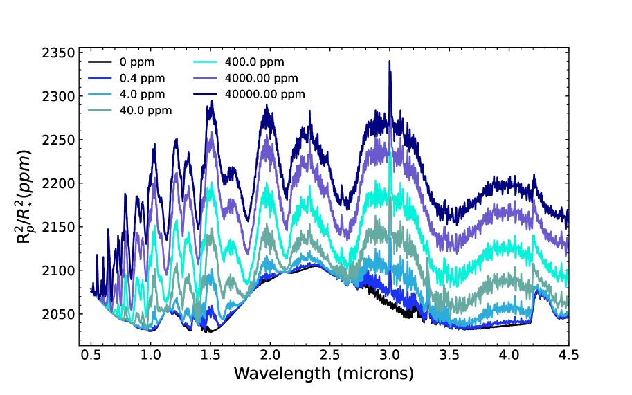
Figure 8: Theoretical transmission spectra of LTT 1445 Ab with varying level of ammonia concentration, 0 ppm, 0.4 ppm, 4.0 ppm, 40 ppm, 400 ppm, 4,000 ppm, and 40,000 ppm

Table 5: NH₃ transmission features for LTT 1445 Ab transmission spectroscopy for varying concentrations of ammonia

Concentration of NH3	Ammonia Feature	S/N	Total <S/N>
	[$\mu$m]	[$\sigma$]	[$\sigma$]
0.4 ppm	1.5	0.10	2.55
	2.0	1.52
	2.3	1.73
	3.0	1.08
4.0 ppm	1.5	1.13	3.10
	2.0	1.56
	2.3	1.75
	3.0	1.67
40 ppm	1.5	2.43	4.34
	2.0	1.92
	2.3	1.98
	3.0	2.30
400 ppm	1.5	3.34	5.32
	2.0	2.33
	2.3	2.22
	3.0	2.59
4000 ppm	1.5	4.15	6.62
	2.0	2.86
	2.3	2.66
	3.0	3.37
40000 ppm	1.5	4.30	6.75
	2.0	2.94
	2.3	2.67
	3.0	3.37

Additionally, we study the impact of clouds on NH₃ detection because clouds are known to exist (e.g. Kreidberg et al. 2014; Helling 2019) and affect transmission spectroscopy observations (e.g. Kitzmann et al. 2010; Benneke et al. 2019). We use petitRADTRANS to model the effects of clouds by setting a gray cloud deck at 1.0, 0.1, and 0.01 bar (Table 6). We choose these gray cloud deck levels because condensation curves for temperate exoplanets indicate that H₂O should condense at pressures below 1.0 bar and form clouds (e.g. Lodders 2003; Marley & Robinson 2015; Tinetti et al. 2018). We find that the presence of clouds even at 1.0 bar lowers the S/N of previously observable NH₃ features to below 3$\sigma$.

Table 6: Average S/N of major NH₃ transmission features for LTT 1445 Ab transmission spectroscopy for varying cloud decks with a H-rich atmosphere

LTT 1445 Ab	Ammonia Feature	S/N	Total <S/N>
	[$\mu$m]	[$\sigma$]	[$\sigma$]
Cloud deck at 0.01 bar	1.5	0.03	0.15
	2.0	0.05
	2.3	0.06
	3.0	0.12
Cloud deck at 0.1 bar	1.5	0.24	0.91
	2.0	0.36
	2.3	0.52
	3.0	0.59
Cloud deck at 1.0 bar	1.5	0.96	2.80
	2.0	1.42
	2.3	1.61
	3.0	1.51

6 Atmospheric Retrieval Results

In this section we investigate how the abundance of NH₃ can be constrained using retrieval analysis. We use petitRADTRANS (Mollière et al., 2020) and PyMultiNest (Buchner et al., 2014) to sample the posteriors. PyMultiNest is the Python version of Multinest for nested sampling (Feroz et al., 2009). In PyMultiNest, we use 2000 live points. Modeling parameters, priors, and retrieval results can be found in Table 7.

6.1 Atmospheric Retrieval Setup

We use the simulated cold Haber world Twinkle data for LTT 1445 Ab as the input (Figure 3 & Table 2). To model the simulated data, we use with the following free parameters: surface gravity, planet radius, temperature for the isothermal atmosphere, cloud deck pressure, and mass mixing ratios for different species that are being considered.

We conduct retrievals for two model setups: (1) a clear atmosphere, (2) an atmosphere with clouds that are parameterized by a grey cloud deck pressure to assess the impact on clouds on the retrieval.

6.2 Fixing Cloud Deck and Other Minor Species

In this case, we use the simulated data for the cloud-free low-mean molecular weight case for LTT 1445 Ab (Figure 3). In the retrieval, we assume the cloud deck at $10^{5}$ bar which assumes an essentially cloud-free case for the retrieval. Given the low abundance/low signal of species other than NH₃, H₂O and CH₄, we fix these species as these species would not be readily detectable. Additionally as with the work in Phillips et al. 2021, we want to check if NH₃ and H₂O can be measured given their overlapping features.

6.2.1 Flat Priors on log (g) and Planetary Radius (R_pl)

We apply a flat prior for the surface gravity and planet radius. As shown in Figure 9, NH₃ and H₂O can be detected in our retrieval, and their abundances are within 1$\sigma$ from the input values. We note that the planetary radius and log (g) are poorly constrained in the case of flat priors. Given that the radius and mass and thus the surface gravity are more precisely constrained by observations (Winters et al., 2021) we introduce Gaussian priors for these values to test the result of our retrieval analysis.

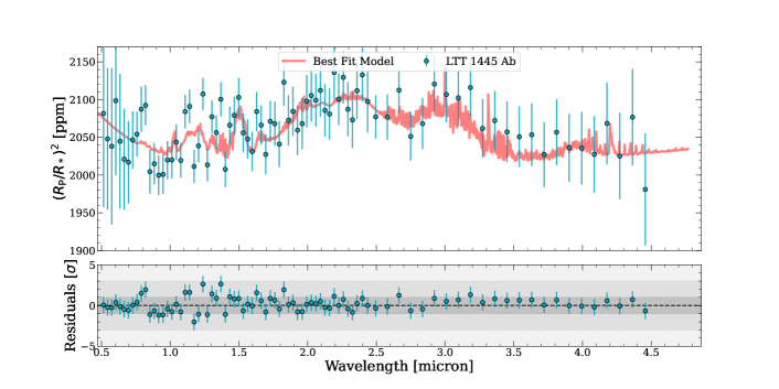
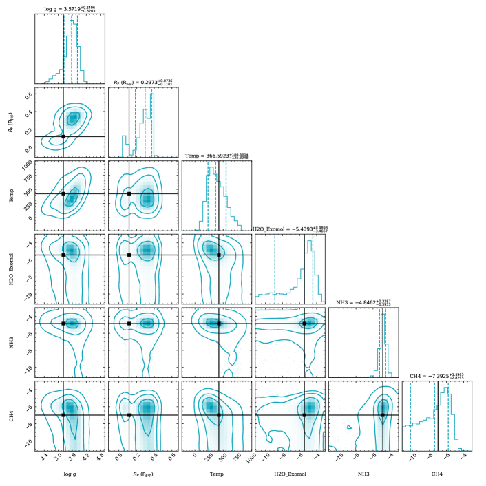
Figure 9: Top: Simulated Twinkle data vs. the retrieved model with flat priors for the surface gravity (log g) and planet radius, and the residuals plotted below. Bottom: Posterior distribution as shown in a corner plot along with the true input values (black lines). Contours are at 1-$\sigma$, 2-$\sigma$, and 3-$\sigma$ from inside out.

6.2.2 Gaussian Priors on log (g) and Planetary Radius (R_pl)

We now consider a retrieval case with Gaussian priors on the log (g) and planetary radius. We apply a Gaussian prior of 3.217$\pm$0.05 dex for log (g) (surface gravity) and 0.1164$\pm$0.005 R_Jup for the planetary radius (Winters et al., 2021). In this case, log g and radius are more tightly constrained because of more constraining priors. Additionally, NH₃ and H₂O are within 1$\sigma$ of their input values. The corner plot and accompanying spectra are shown in Figure 10. Retrieval results can be found in Table 7.

To quantify the detection significance, we use similar methods as in Phillips et al. (2021). Given the 11,611 posterior samples, there are $\sim$0.75 per cent that have a lower value than 10^-8 mixing ratio for NH₃. The 10^-8 mixing ratio threshold is chosen because below this value it is difficult for our retrieval code to constrain abundances (e.g., CH₄). The 0.75 per cent fraction translates to 2.6-$\sigma$ assuming a normal distribution. This is consistent with the 3.1-$\sigma$ detection significance from the SNR analysis in §5.

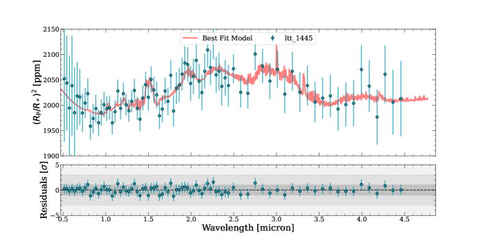
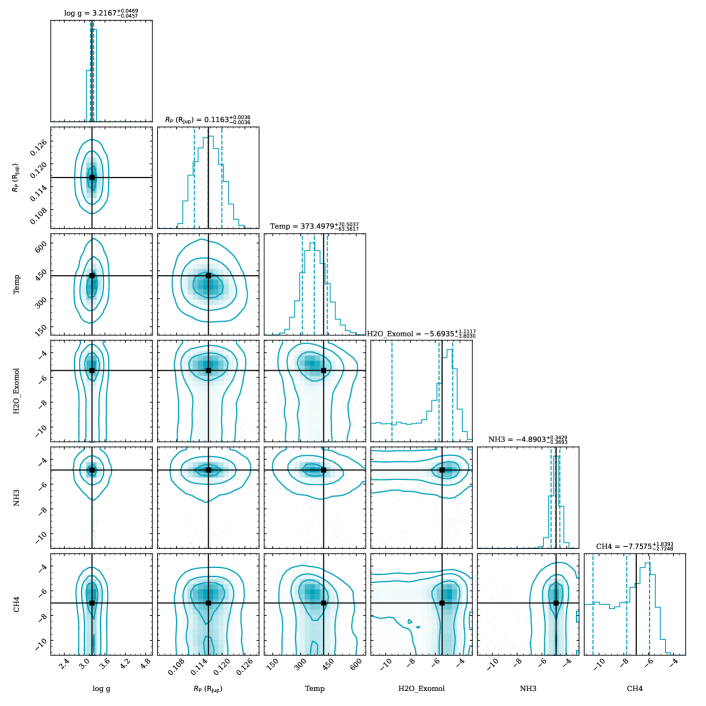
Figure 10: Same as Figure. 9 but with Gaussian priors for the surface gravity (log g) and planet radius.

6.3 Cloud Deck as a Free Parameter

Following Phillips et al. (2021), we also run a retrieval analysis on the full parameter set that includes (1) the cloud deck pressure; and (2) all minor species other than NH₃, H₂O and CH₄. The prior for the cloud deck pressure covers a range from $10^{-4}$ to $10^{7}$ bar. We are able to put an upper limit to the cloud deck pressure at $\sim$100 bar at at a 1$\sigma$ level. We are unable to constrain minor species with mixing ratio lower than 10^-8, but we can constrain NH₃ within 1$\sigma$ of the input value. The results are in Table 7 and the corner plot is shown in Figure 11.

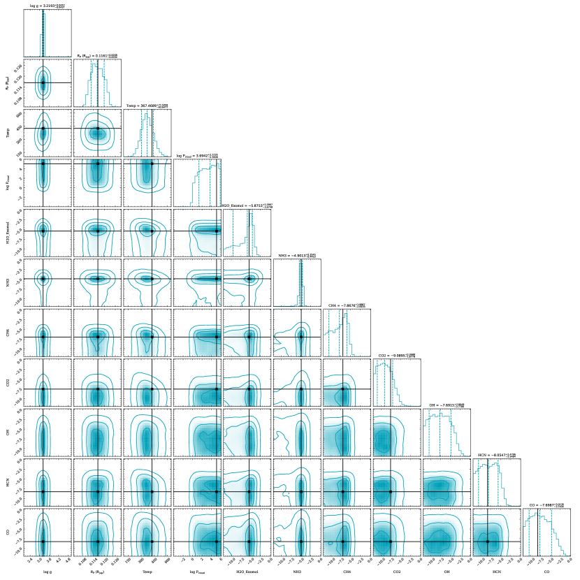
Figure 11: Corner plot for the full parameter set along with true values (black lines) that are used in generating the Twinkle data.

7 Summary and Conclusions

We model the terrestrial-like planet LTT 1445 Ab for the detection of the potential biosignature ammonia with the upcoming Twinkle mission. LTT 1445 Ab is modeled using petitRADTRANS and TwinkleRad. A baseline of 25 transits, 4.0 ppm concentration of NH₃, and a H-rich atmosphere is considered to determine whether NH₃ is detectable.

We demonstrate that Twinkle will have the capabilities to distinguish between a cold Haber world and a Hycean world scenario (§4). Given the modeled spectra and the associated uncertainties, we find a $\chi_{\nu}^{2}$ = 3.01, indicating that Twinkle can differentiate the two worlds. Interior composition analysis indicates that LTT 1445 Ab is likely not a Hycean world. This planet is more consistent with a rocky planet without a substantial water mass fraction.

We explore the fraction of hydrogen needed in the atmosphere of LTT 1445 Ab for ammonia to be detectable (§5). We find that in order to detect NH₃, LTT 1445 Ab would need a significant portion of H₂ in the atmosphere (H₂ = 90 per cent). We also explore the effects on cloud decks and the concentration of NH₃ on the detectability of NH₃ in the atmosphere. We find that even the presence of a cloud deck at 1.0 bar would reduce the overall S/N to be lower than 3-$\sigma$ for NH₃ detection. In addition, we find that a 4.0 ppm concentration of NH₃ is needed to be detectable by Twinkle.

Lastly, we conduct atmospheric retrieval analysis (§6) which provides helpful insight into constraining NH₃ and H₂O given optimal conditions (i.e a cloud free atmosphere with low MMW). We find that NH₃ can be detected at 2.6$-\sigma$. This is consistent with our quadrature sum <S/N> estimate of 3.10$\sigma$.

This work demonstrates that Twinkle can provide useful characterization of promising potential smaller terrestrial-like planets to provide insights into potential biosignatures and atmospheric characterization.

References

- Al-Refaie et al. (2021) Al-Refaie A. F., Changeat Q., Waldmann I. P., Tinetti G., 2021, ApJ, 917, 37
- Benneke et al. (2019) Benneke B., et al., 2019, Nature Astronomy, 3, 813
- Borucki et al. (2010) Borucki W. J., et al., 2010, Science, 327, 977
- Buchner et al. (2014) Buchner J., et al., 2014, A&A, 564, A125
- Catling et al. (2018) Catling D. C., et al., 2018, Astrobiology, 18, 709
- Chouqar et al. (2020) Chouqar J., Benkhaldoun Z., Jabiri A., Lustig-Yaeger J., Soubkiou A., Szentgyorgyi A., 2020, MNRAS, 495, 962
- Diamond-Lowe et al. (2018) Diamond-Lowe H., Berta-Thompson Z., Charbonneau D., Kempton E. M. R., 2018, AJ, 156, 42
- Diamond-Lowe et al. (2020) Diamond-Lowe H., Berta-Thompson Z., Charbonneau D., Dittmann J., Kempton E. M. R., 2020, AJ, 160, 27
- Dittmann et al. (2017) Dittmann J. A., et al., 2017, Nature, 544, 333
- Edwards & Stotesbury (2021) Edwards B., Stotesbury I., 2021, AJ, 161, 266
- Edwards et al. (2019) Edwards B., et al., 2019, Experimental Astronomy, 47, 29
- Edwards et al. (2021) Edwards B., et al., 2021, AJ, 161, 44
- Feroz et al. (2009) Feroz F., Hobson M. P., Bridges M., 2009, MNRAS, 398, 1601
- Fressin et al. (2013) Fressin F., et al., 2013, ApJ, 766, 81
- Fulton et al. (2017) Fulton B. J., et al., 2017, AJ, 154, 109
- Gillon et al. (2017) Gillon M., et al., 2017, Nature Astronomy, 1, 0056
- Ginzburg et al. (2018) Ginzburg S., Schlichting H. E., Sari R., 2018, MNRAS, 476, 759
- Gupta & Schlichting (2021) Gupta A., Schlichting H. E., 2021, MNRAS, 504, 4634
- Helling (2019) Helling C., 2019, Annual Review of Earth and Planetary Sciences, 47, 583
- Hu et al. (2021) Hu R., Damiano M., Scheucher M., Kite E., Seager S., Rauer H., 2021, ApJ, 921, L8
- Huang et al. (2021) Huang J., Seager S., Petkowski J. J., Ranjan S., Zhan Z., 2021, arXiv e-prints, p. arXiv:2107.12424
- Kempton et al. (2018) Kempton E. M. R., et al., 2018, PASP, 130, 114401
- Kitzmann et al. (2010) Kitzmann D., Patzer A. B. C., von Paris P., Godolt M., Stracke B., Gebauer S., Grenfell J. L., Rauer H., 2010, A&A, 511, A66
- Kreidberg et al. (2014) Kreidberg L., et al., 2014, Nature, 505, 69
- Lodders (2003) Lodders K., 2003, ApJ, 591, 1220
- Lopez & Fortney (2013) Lopez E. D., Fortney J. J., 2013, ApJ, 776, 2
- Madhusudhan et al. (2021) Madhusudhan N., Piette A. A. A., Constantinou S., 2021, arXiv e-prints, p. arXiv:2108.10888
- Marcus et al. (2010) Marcus R. A., Sasselov D., Hernquist L., Stewart S. T., 2010, ApJ, 712, L73
- Marley & Robinson (2015) Marley M. S., Robinson T. D., 2015, ARA&A, 53, 279
- Miller-Ricci et al. (2008) Miller-Ricci E., Seager S., Sasselov D., 2008, The Astrophysical Journal, 690, 1056–1067
- Mollière et al. (2019) Mollière P., Wardenier J. P., van Boekel R., Henning T., Molaverdikhani K., Snellen I. A. G., 2019, A&A, 627, A67
- Mollière et al. (2020) Mollière P., et al., 2020, A&A, 640, A131
- Mugnai et al. (2020) Mugnai L. V., Pascale E., Edwards B., Papageorgiou A., Sarkar S., 2020, Experimental Astronomy, 50, 303
- Nixon & Madhusudhan (2021) Nixon M. C., Madhusudhan N., 2021, Monthly Notices of the Royal Astronomical Society, 505, 3414
- Owen & Wu (2017) Owen J. E., Wu Y., 2017, ApJ, 847, 29
- Phillips et al. (2021) Phillips C., Wang J., Kendrew S., Greene T. P., Hu R., Valenti J., Panero W. R., Schulze J., 2021, arXiv e-prints, p. arXiv:2109.12132
- Ranjan et al. (2022) Ranjan S., Seager S., Zhan Z., Koll D. D. B., Bains W., Petkowski J. J., Huang J., Lin Z., 2022, arXiv e-prints, p. arXiv:2201.08359
- Ricker et al. (2015) Ricker G. R., et al., 2015, Journal of Astronomical Telescopes, Instruments, and Systems, 1, 014003
- Schulze et al. (2020) Schulze J. G., Wang J., Johnson J. A., Unterborn C. T., Panero W. R., 2020, arXiv e-prints, p. arXiv:2011.08893
- Seager et al. (2013a) Seager S., Bains W., Hu R., 2013a, ApJ, 775, 104
- Seager et al. (2013b) Seager S., Bains W., Hu R., 2013b, ApJ, 777, 95
- Stotesbury et al. (2022) Stotesbury I., et al., 2022, arXiv e-prints, p. arXiv:2209.03337
- Suissa et al. (2018) Suissa G., Chen J., Kipping D., 2018, MNRAS, 476, 2613
- Tinetti et al. (2018) Tinetti G., et al., 2018, Experimental Astronomy, 46, 135
- Tsai et al. (2021) Tsai S.-M., Innes H., Lichtenberg T., Taylor J., Malik M., Chubb K., Pierrehumbert R., 2021, arXiv e-prints, p. arXiv:2111.06429
- Unterborn et al. (2018) Unterborn C. T., Desch S. J., Hinkel N. R., Lorenzo A., 2018, Nature Astronomy, 2, 297
- Van Eylen et al. (2018) Van Eylen V., Agentoft C., Lundkvist M. S., Kjeldsen H., Owen J. E., Fulton B. J., Petigura E., Snellen I., 2018, MNRAS, 479, 4786
- Winters et al. (2019) Winters J. G., et al., 2019, AJ, 158, 152
- Winters et al. (2021) Winters J. G., et al., 2021, arXiv e-prints, p. arXiv:2107.14737
- Wunderlich et al. (2020) Wunderlich F., Scheucher M., Grenfell J. L., Schreier F., Sousa-Silva C., Godolt M., Rauer H., 2020, arXiv e-prints, p. arXiv:2012.11426
- Zeng & Jacobsen (2017) Zeng L., Jacobsen S. B., 2017, ApJ, 837, 164
- Zeng & Sasselov (2013) Zeng L., Sasselov D., 2013, PASP, 125, 227
- Zeng et al. (2016) Zeng L., Sasselov D. D., Jacobsen S. B., 2016, ApJ, 819, 127
- Zeng et al. (2019) Zeng L., et al., 2019, Proceedings of the National Academy of Science, 116, 9723