Relativistic corrections to paired production of charmonium and bottomonium in decays of the Higgs boson

Abstract

Rare decay process of the Higgs boson into a pair of $J/\Psi$ and $\Upsilon$ particles is studied within perturbative Standard Model and relativistic quark model. The relativistic corrections connected with the relative motion of quarks are calculated in the production amplitude and the wave functions of the bound states. Numerical values of the decay widths of the Higgs boson are obtained, which can be used for comparison with experimental data.

I Introduction

After the discovery of the Higgs boson atlas ; cms , a period of detailed study of the processes connected with this particle was begun. We can say that the study of the Higgs sector has become one of the most important areas in particle physics cms1 . The discovery of the Higgs boson confirmed the electroweak mechanism of symmetry breaking, but the nature of this particle remains to be explored. To do this, it is necessary to create particle colliders, on which Higgs bosons could be produced in significant quantities, which would make it possible to proceed to a precise study of the parameters of the Higgs sector. It is possible that interaction processes involving the Higgs boson can provide a transition to a New Physics that lies beyond the Standard Model.

Among the parameters of the Higgs sector, the coupling constants of the Higgs boson with various bosons g(HZZ), g(HWW), leptons $g(H\tau\tau)$, $g(H\mu\mu)$ and quarks g(Hcc), g(Hbb) stand out. They determine the decay processes of the Higgs boson into various particles pdg . Due to its large mass and the presence of coupling constants with different particles, the Higgs boson has numerous decay channels. The decay channel of the Higgs boson into a pair of heavy quarks is interesting because it creates the possibility of the production of bound states of heavy quarks. Thus, rare exclusive decay processes of the Higgs boson into a pair of charmonium or bottomonium are of obvious interest both for studying the decay mechanisms and for studying the properties of bound states of quarks.

The CMS collaboration began the search for rare Higgs decays into a pair of heavy vector quarkonia in 2019 cms2 . The results of new upper limits on the branching fractions are obtained in cms3 :

$$B(H\to J/\Psi,J/\Psi)<3.8\cdot 10^{-4},$$ (1)

$$B(H\to\Upsilon(1S),\Upsilon(1S))<1.7\cdot 10^{-3}.$$ (2)

Theoretical studies of the production of a pair of heavy quarkonia in the decays of the Higgs boson began about 40 years ago in bander ; keung . In these papers, theoretical formulas were obtained for estimating the decay widths in the nonrelativistic approximation for some decay mechanisms. Relatively more recent theoretical studies of these processes have been carried out in luchinsky ; apm2021 ; apm2022 ; neng .

In this work we continue the study of relativistic effects in the exclusive paired charmonium and bottomonium production in the Higgs boson decay which was begun in apm2021 ; apm2022 for $B_{c}$ mesons. Our calculation of the decay widths is performed on the basis of relativistic quark model used previously for the investigation of relativistic corrections in different reactions in apm1 ; apm2 ; apm3 . Despite the rare nature of the Higgs boson decays being studied, one can hope that such processes can be investigated at the new Higgs boson factories. The aim of the present work is to give new analysis of pair quarkonium production in Higgs boson decays in the Standard Model:

1. In comparison with previous works luchinsky ; neng we consider different production mechanisms (quark-gluon, quark-photon, photon-photon and Z-boson mechanisms) of the pair charmonium and bottomonium production.

2. We take into account relativistic corrections connected with the relative motion of heavy quarks both in the pair production amplitude itself and in the wave functions of the bound states.

As a result, new numerical estimation for the Higgs boson decay rates is obtained. An experimental study of these rare decays of the Higgs boson at future high-luminosity accelerators could be useful in testing the Standard Model with greater accuracy.

II General formalism

From the very beginning, it should be emphasized that there are several groups of amplitudes for the decay of the Higgs boson with the formation of a pair of charmoniums $J/\Psi$ (bottomonium $\Upsilon$), which contribute the same order of magnitude to the decay width. We study the amplitudes which are shown in Fig. 1-Fig. 5 and representing different decay mechanisms with pair vector meson production: quark-gluon, quark-photon, quark-loop, W-boson loop and Z-boson. The first group includes quark-gluon amplitudes shown in Fig. 1 (quark-gluon mechanism). The factor determining the order of contributions can be represented as $\alpha_{s}/M_{H}^{4}$, where $M_{H}$ is the mass of the Higgs boson. Such a factor can be distinguished from the very beginning due to the structure of the interaction vertices and the denominators of the particle propagators. The second group is formed by quark-photon amplitudes shown in Fig. 2 (quark-photon mechanism). The order of contribution is determined here by the following factor $\alpha/M_{H}^{2}M_{{\cal Q\bar{Q}}}^{2}$. The third group is formed by the amplitudes in Fig. 3-Fig. 4 which contain the quark or W-boson loop with two photons that create a pair of $J/\Psi$ (or $\Upsilon$) mesons (quark-loop and W-boson loop mechanisms). The primary common factor in this case takes the form $\alpha^{2}/M_{{\cal Q\bar{Q}}}^{4}$. Finally, the last group of amplitudes in Fig. 5 is determined by the interaction of the Higgs boson with a pair of Z-bosons (Z-boson mechanism). To achieve good calculation accuracy, it is necessary to take into account the contribution of all amplitudes from these groups in Fig. 1-Fig. 5.

Let consider firstly the Higgs boson decay amplitudes shown in Fig. 1, 2. For pair production of quarkonia in the leading order of perturbation theory, it is necessary to obtain at the first stage two free quarks and two free antiquarks. Then they can form bound states with some probability at the next stage. In the quasipotential approach the decay amplitude can be presented as a convolution of a perturbative production amplitude of two $c$-quark and $\bar{c}$-antiquark pairs and the quasipotential wave functions of the final mesons apm2021 ; apm2022 :

$${\cal M}(P,Q)=-i(\sqrt{2}G_{F})^{\frac{1}{2}}\frac{2\pi}{3}M_{{\cal{Q\bar{Q}}}}\int\frac{d{\bf p}}{(2\pi)^{3}}\int\frac{d{\bf q}}{(2\pi)^{3}}\times$$ (3)

$$\times Tr\left\{\Psi^{\cal V}(p,P)\Gamma_{1}^{\nu}(p,q,P,Q)\Psi^{\cal V}(q,Q)\gamma_{\nu}+\Psi^{\cal V}(q,Q)\Gamma_{2}^{\nu}(p,q,P,Q)\Psi^{\cal V}(p,P)\gamma_{\nu}\right\},$$

where $M_{{\cal{Q\bar{Q}}}}$ is the mass of quarkonium, Four-momenta $p_{1}$ and $p_{2}$ of $c$-quark and $\bar{c}$-antiquark in the pair forming the first ${\cal(Q\bar{Q})}$ meson, and four-momenta $q_{2}$ and $q_{1}$ for quark and antiquark in the second meson ${\cal(Q\bar{Q})}$ are expressed in terms of relative and total four momenta as follows:

$$p_{1,2}=\frac{1}{2}P\pm p,\quad(pP)=0;\qquad q_{1,2}=\frac{1}{2}Q\pm q,\quad(qQ)=0,$$ (4)

A superscript ${\cal P}$ indicates a pseudoscalar meson ${\cal(Q\bar{Q})}$, a superscript ${\cal V}$ indicates a vector meson ${\cal(Q\bar{Q})}$. The vertex functions $\Gamma_{1,2}$ are presented below in leading order and in Fig. 1. Heavy quarks $c$, $b$ and antiquarks $\bar{c}$, $\bar{b}$ are outside the mass shell in the intermediate state: $p_{1,2}^{2}\not=m^{2}$, so that $p_{1}^{2}-m^{2}=p_{2}^{2}-m^{2}$, which means that there is a symmetrical exit of particles from the mass shell.

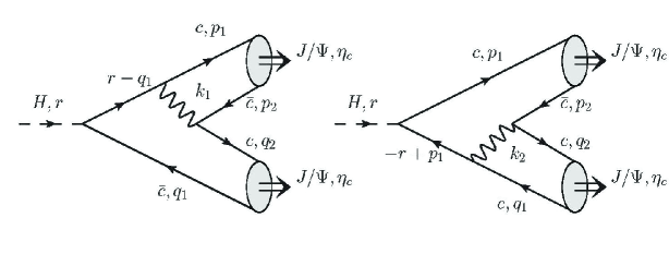
Figure 1: Quark-gluon mechanism of the pair charmonium production in the Higgs boson decay. Dashed line shows the Higgs boson and wavy line corresponds to the gluon.

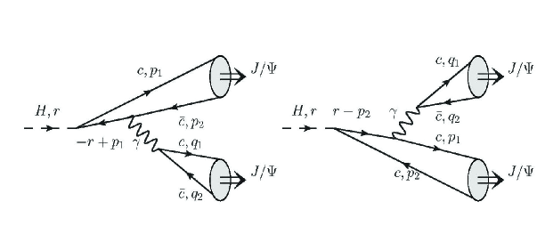
Figure 2: Quark-photon mechanism of the pair charmonium production in the Higgs boson decay. Dashed line shows the Higgs boson and wavy line corresponds to the photon.

In Eq. (3) we integrate over the relative three-momenta of quarks and antiquarks in the final state. The systematic account of all terms depending on the relative quark momenta $p$ and $q$ in the decay amplitude is important for increasing the accuracy of the calculation. $p=L_{P}(0,\mathbf{p})$ and $q=L_{Q}(0,\mathbf{q})$ are the relative four-momenta obtained by the Lorentz transformation of four-vectors $(0,\mathbf{p})$ and $(0,\mathbf{q})$ to the reference frames moving with the four-momenta $P$ and $Q$.

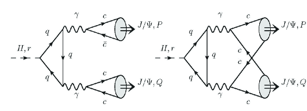
Figure 3: Quark loop mechanism of the pair charmonium production in the Higgs boson decay. Dashed line shows the Higgs boson and wavy line corresponds to the photon.

The relativistic wave functions of the bound quarks accounting for the transformation from the rest frame to the moving one with four momenta $P$, and $Q$, are

$$\Psi(p,P)=\frac{\Psi_{0}(\mathbf{p})}{\bigl{[}\frac{\epsilon(p)}{m}\frac{\epsilon(p)+m}{2m}\bigr{]}}\left[\frac{\hat{v}_{1}-1}{2}+\hat{v}_{1}\frac{\mathbf{p}^{2}}{2m(\epsilon(p)+m)}-\frac{\hat{p}}{2m}\right]\times\\ \hat{\varepsilon}(P,S_{z})$$ (5)

$$(1+\hat{v}_{1})\left[\frac{\hat{v}_{1}+1}{2}+\hat{v}_{1}\frac{\mathbf{p}^{2}}{2m(\epsilon(p)+m)}+\frac{\hat{p}}{2m}\right],$$

$$\Psi(q,Q)=\frac{\Psi_{0}(\mathbf{q})}{\bigl{[}\frac{\epsilon(q)}{m}\frac{\epsilon(q)+m}{2m}\bigr{]}}\left[\frac{\hat{v}_{2}-1}{2}+\hat{v}_{2}\frac{\mathbf{q}^{2}}{2m(\epsilon(q)+m)}+\frac{\hat{q}}{2m}\right]\times\\ \hat{\varepsilon}(Q,S_{z})$$ (6)

$$(1+\hat{v}_{2})\left[\frac{\hat{v}_{2}+1}{2}+\hat{v}_{2}\frac{\mathbf{q}^{2}}{2m(\epsilon(q)+m)}-\frac{\hat{q}}{2m}\right],$$

where the hat symbol means a contraction of the four–vector with the Dirac gamma matrices; $v_{1}=P/M_{{\cal{Q\bar{Q}}}}$, $v_{2}=Q/M_{{\cal{Q\bar{Q}}}}$; $\epsilon(p)=\sqrt{m^{2}+\mathbf{p}^{2}}$, $m$ is $c(b)$-quark mass, and $M_{{\cal{Q\bar{Q}}}}$ is the mass of charmonium (bottomonium) state. $\varepsilon^{\lambda}(P,S_{z})$ is the polarization vector of the $J/\Psi(\Upsilon)$ meson.

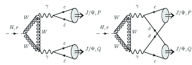
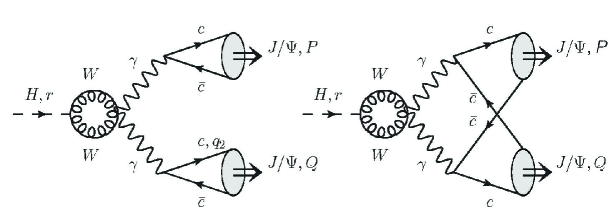
Figure 4: W-boson loop mechanism of the pair charmonium production in the Higgs boson decay. Dashed line shows the Higgs boson and wavy line corresponds to the photon.

Expressions (5) and (6) represent complicated functions depending on relative momenta ${\bf p}$, ${\bf q}$ including the bound state wave function in the rest frame $\Psi_{0}({\bf p})$. The color part of the meson wave function in the amplitudes (5)-(6) is taken as $\delta_{ij}/\sqrt{3}$ (color indexes $i,j,k=1,2,3$).

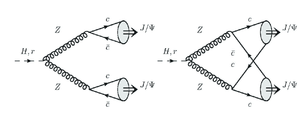
Figure 5: Z-boson mechanism of the pair charmonium production in the Higgs boson decay. Dashed line shows the Higgs boson and wavy line corresponds to the Z-boson.

The general structure of expressions (5)-(6) allows us to say that they are the product of the wave functions of mesons in the rest frame and special projection operators resulting from the transformation from the moving reference frame to the reference frame in which the meson is at rest. Expressions (5)-(6) make it possible to correctly take into account the relativistic corrections connected with the relative momenta of quarks in the final states. It is useful to note that the expression for the projection operators was obtained in the framework of nonrelativistic quantum chromodynamics in bodwin2002 in a slightly different form for the case when the quark momenta lie on the mass shell. The transformation law of the bound state wave functions of quarks, which is used in the derivation of equations (5)-(6) , was obtained in the Bethe-Salpeter approach in brodsky and in quasipotential method in faustov .

As follows from (5)-(6), when constructing the decay amplitudes of the Higgs boson, projection operators are introduced for quark-antiquark pairs onto the spin states with total spin $S=1$ of the following form:

$$\hat{\Pi}^{\cal V}=[v_{2}(0)\bar{u}_{1}(0)]_{S=1}=\hat{\varepsilon}\frac{1+\gamma^{0}}{2\sqrt{2}}.$$ (7)

Total amplitude of the Higgs boson decay to paired vector quarkonium in the case of quark-gluon mechanism in the leading order in strong coupling constant $\alpha_{s}$ can be presented in the form:

$${\mathcal{M}}=\frac{4\pi}{3}M_{{\cal{Q\bar{Q}}}}\alpha_{s}\Gamma_{Q}\int\!\frac{d\mathbf{p}}{(2\pi)^{3}}\int\!\frac{d\mathbf{q}}{(2\pi)^{3}}\mathrm{Tr}\bigl{\{}\mathcal{T}_{12}+\mathcal{T}_{34}\bigr{\}},$$ (8)

$${\mathcal{T}_{12}}=\Psi^{\cal V}(p,P)\left[\frac{\hat{p}_{1}-\hat{r}+m}{(r-p_{1})^{2}-m^{2}}\,\gamma_{\mu}+\gamma_{\mu}\,\frac{\hat{r}-\hat{q}_{1}+m}{(r-q_{1})^{2}-m^{2}}\right]D^{\mu\nu}(k_{2})\Psi^{\cal V}(q,Q)\gamma_{\nu},$$ (9)

$${\mathcal{T}_{34}}=\Psi^{\cal V}(q,Q)\left[\frac{\hat{p}_{2}-\hat{r}+m}{(r-p_{2})^{2}-m^{2}}\,\gamma_{\mu}+\gamma_{\mu}\frac{\hat{r}-\hat{q}_{2}+m}{(r-q_{2})^{2}-m^{2}}\,\right]D^{\mu\nu}(k_{1})\Psi^{\cal V}(p,P)\gamma_{\nu},$$ (10)

where $\alpha_{s}=\alpha_{s}\left(\frac{M_{H}^{2}}{4\Lambda^{2}}\right)$, $\Gamma_{Q}=m(\sqrt{2}G_{F})^{\frac{1}{2}}$.

Four-momentum of Higgs boson squared $r^{2}=M_{H}^{2}=(P+Q)^{2}=2M_{{\cal{Q\bar{Q}}}}^{2}+2PQ$, the gluon four-momenta are $k_{1}=p_{1}+q_{1}$, $k_{2}=p_{2}+q_{2}$. Relative momenta $p$, $q$ of heavy quarks enter in the gluon propagators $D_{\mu\nu}(k_{1,2})$ and quark propagators as well as in relativistic wave functions (5) and (6). Accounting for the small ratio of relative quark momenta $p$ and $q$ to the mass of the Higgs boson $M_{H}$, we can simplify the inverse denominators of quark and gluon propagators as follows:

$$\frac{1}{(p_{1}+q_{1})^{2}}\approx\frac{1}{(p_{2}+q_{2})^{2}}=\frac{4}{M_{H}^{2}},$$ (11)

$$\frac{1}{(r-q_{1})^{2}-m_{1}^{2}}=\frac{1}{(-r-p_{1})^{2}-m_{1}^{2}}=\frac{1}{(r-p_{2})^{2}-m_{1}^{2}}=\frac{1}{(-r-q_{2})^{2}-m_{1}^{2}}=\frac{2}{M_{H}^{2}}.$$ (12)

In (11)-(12) we completely neglect corrections of the form $|{\bf p}|/M_{H}$, $|{\bf q}|/M_{H}$. At the same time, we keep in the amplitudes (9), (10) the second-order correction for small ratios $|{\bf p}|/m$, $|{\bf q}|/m$ relative to the leading order result. Calculating the trace in obtained expression in the package FORM form , we find relativistic amplitudes of the paired meson production in the form:

$${\cal M_{VV}}^{(1)}=\frac{256\pi}{3M_{H}^{4}}(\sqrt{2}G_{F})^{\frac{1}{2}}mM_{{\cal{Q\bar{Q}}}}\alpha_{s}\varepsilon_{1}^{\lambda}\varepsilon_{2}^{\sigma}F_{1,{\cal VV}}^{\lambda\sigma}|\tilde{\Psi}_{\cal V}(0)|^{2},$$ (13)

where $\varepsilon_{1}^{\lambda}$, $\varepsilon_{2}^{\sigma}$ are the polarization vectors of spin 1 mesons. The superscript in amplitude designation and subscript in tensor function $F_{{\cal VV}}$ designation denotes the contribution of the quark-gluon mechanism in Fig. 1.

The contribution of the amplitudes in Fig. 2 must also be taken into account, since these amplitudes have the same order as the previous ones, despite the replacement $\alpha_{s}\to\alpha$. This is due to the presence in the denominator of the mass of the meson instead of the mass of the Higgs boson bodwin2014 . The expression for the production amplitudes of the pair $J/\Psi$ has a similar structure with slight changes in the common factors:

$${\cal M_{VV}}^{(2)}=\frac{288\pi}{M_{H}^{2}M_{\cal{Q\bar{Q}}}}(\sqrt{2}G_{F})^{\frac{1}{2}}me_{Q}^{2}\alpha\varepsilon_{1}^{\lambda}\varepsilon_{2}^{\sigma}F_{2,{\cal VV}}^{\lambda\sigma}|\tilde{\Psi}_{\cal V}(0)|^{2}.$$ (14)

The tensor corresponding to the quark or W-boson loops in Fig. 3-Fig. 4 has the structure (the subscript denotes the contribution of the quark or bosonic loop):

$$T^{\mu\nu}_{Q,W}=A_{Q,W}(t)(g^{\mu\nu}(v_{1}v_{2})-v_{1}^{\nu}v_{2}^{\mu})+B_{Q,W}(t)[v_{2}^{\mu}-v_{1}^{\mu}(v_{1}v_{2})][v_{1}^{\nu}-v_{2}^{\nu}(v_{1}v_{2})],$$ (15)

where $t=\frac{M_{h}^{2}}{4m_{Q}^{2}}$ or $t=\frac{M_{h}^{2}}{4m_{W}^{2}}$. The structure functions $A_{Q,W}(t)$, $B_{Q,W}(t)$ can be obtained using an explicit expression for a loop integrals (see Appendix A,B).

The amplitudes in Fig. 3-5 with quark, W-boson loops and $ZZ$ in an intermediate state contain the contributions of direct and crossed diagrams. In this case, direct diagrams, in which virtual photons or Z-bosons give vector quarkonia in the final state, are dominant in terms of the mass factor. However, the structure of the numerators of the direct and cross amplitudes is different, which can eventually lead to numerically close contributions. In what follows, we present the expressions for these amplitudes only in the leading order:

$${\cal M_{VV}}^{(3)}=\frac{2052\pi^{2}}{m_{Q}M_{\cal{Q\bar{Q}}}}(\sqrt{2}G_{F})^{\frac{1}{2}}e_{q}^{2}e_{Q}^{2}\alpha^{2}\varepsilon_{1}^{\lambda}\varepsilon_{2}^{\sigma}F_{3,{\cal VV}}^{\lambda\sigma}|\tilde{\Psi}_{\cal V}(0)|^{2},$$ (16)

$${\cal M_{VV}}^{(4)}=\frac{48\pi^{2}M_{Z}M_{W}}{M^{4}_{\cal{Q\bar{Q}}}}(\sqrt{2}G_{F})^{\frac{1}{2}}e_{q}^{2}\alpha^{2}\cos\theta_{W}\varepsilon_{1}^{\lambda}\varepsilon_{2}^{\sigma}F_{4,{\cal VV}}^{\lambda\sigma}|\tilde{\Psi}_{\cal V}(0)|^{2},$$ (17)

$${\cal M_{VV}}^{(5)}=\frac{48\pi\alpha}{M_{Z}^{2}\sin^{2}2\theta_{W}}(\sqrt{2}G_{F})^{\frac{1}{2}}\varepsilon_{1}^{\lambda}\varepsilon_{2}^{\sigma}F_{5,{\cal VV}}^{\lambda\sigma}|\tilde{\Psi}_{\cal V}(0)|^{2},$$ (18)

where $m$ is the mass of heavy quark c, b, produced in the vertex of Higgs boson decay, $m_{Q}$ is the heavy quark mass in quark loop, $e_{q}$ is the charge (in units e) of heavy quark (c or b) entering in final mesons, $e_{Q}$ is the charge (in units e) of heavy quark (c or b) in the quark loop.

The tensor functions in amplitudes (13)-(18) have the following form:

$$F^{\alpha\beta}_{i,{\cal VV}}=g^{(i)}_{1}v_{1}^{\alpha}v_{2}^{\beta}+g^{(i)}_{2}g^{\alpha\beta},~{}~{}~{}g^{(1)}_{1}=-2+\frac{2}{9}\omega_{1}^{2},$$ (19)

$$g^{(1)}_{2}=-1-2r_{2}+r_{1}^{2}+\frac{4}{3}r_{2}\omega_{1}+\frac{1}{9}\omega_{1}^{2}+\frac{2}{3}r_{2}\omega_{1}^{2}-\frac{1}{9}r_{1}^{2}\omega_{1}^{2},$$

$$g^{(2)}_{1}=4-\frac{4}{9}\omega_{1}^{2},~{}g^{(2)}_{2}=2+4r_{2}-2r_{1}^{2}-\frac{8}{3}r_{2}\omega_{1}-\frac{2}{9}\omega_{1}^{2}-\frac{4}{3}r\omega_{1}^{2}+\frac{2}{9}r_{1}^{2}\omega_{1}^{2},$$ (20)

$$g^{(3)}_{1,Q}=-A_{Q}(t)(1+\frac{2}{3}\omega_{1}+\frac{1}{9}\omega_{1}^{2})+B_{Q}(t)(1+\frac{2}{3}\omega_{1}+\frac{1}{9}\omega_{1}^{2}),~{}$$ (21)

$$g^{(3)}_{2,Q}=A_{Q}(t)\left(-1-\frac{2}{3}\omega_{1}-\frac{1}{9}\omega_{1}^{2}+\frac{1}{2}r_{1}^{2}+\frac{1}{3}\omega_{1}r_{1}^{2}+\frac{1}{18}\omega_{1}^{2}r_{1}^{2}\right),$$

$$g^{(4)}_{1}=-A_{W}(t)\left(1+\frac{2}{3}\omega_{1}+\frac{1}{9}\omega_{1}^{2}\right)+B_{W}(t)\left(1+\frac{2}{3}\omega_{1}+\frac{1}{9}\omega_{1}^{2}\right),$$ (22)

$$g^{(4)}_{2}=A_{W}(t)\left(-1-\frac{2}{3}\omega_{1}-\frac{1}{9}\omega_{1}^{2}+\frac{1}{2}r_{1}^{2}+\frac{1}{3}\omega_{1}r_{1}^{2}+\frac{1}{18}\omega_{1}^{2}r_{1}^{2}\right),~{}$$ (23)

$$g^{(5)}_{2}=\left(1+\frac{1}{3}\omega_{1}\right)^{2}\left(\frac{1}{2}-a_{z}\right)^{2}-\frac{M_{z}^{4}}{3\left(\frac{M_{h}^{2}}{4}-M_{Z}^{2}\right)^{2}}\Bigl{(}-\frac{1}{4}-\frac{1}{6}\omega_{1}-\frac{1}{36}\omega_{1}^{2}+$$ (24)

$$+\frac{1}{2}a_{z}+\frac{1}{3}\omega_{1}a_{z}+\frac{1}{18}\omega_{1}^{2}a_{z}-\frac{1}{2}a_{z}^{2}-\frac{1}{3}\omega_{1}a_{z}^{2}-\frac{1}{18}\omega_{1}^{2}a_{z}^{2}\Bigr{)},~{}~{}~{}g^{(5)}_{1}=0,$$

where the parameter $r_{1}=\frac{M_{H}}{M_{{\cal Q\bar{Q}}}}$, $r_{2}=\frac{m}{M_{{\cal Q\bar{Q}}}}$, $a_{z}=2|e_{Q}|\sin^{2}\theta_{W}$.

The decay widths of the Higgs boson into a pair of vector quarkonia states are determined by the following expressions (see also apm2021 ; apm2022 ):

$$\Gamma_{\cal{VV}}=\frac{2^{14}\sqrt{2}\pi\alpha_{s}^{2}m^{2}G_{F}|\tilde{\Psi}_{\cal V}(0)|^{4}\sqrt{\frac{r_{1}^{2}}{4}-1}}{9M_{H}^{5}r_{1}^{5}}\sum_{\lambda,\sigma}|\varepsilon_{1}^{\lambda}\varepsilon_{2}^{\sigma}F^{\lambda\sigma}_{{\cal VV}}|^{2},$$ (25)

$$F^{\lambda\sigma}_{{\cal VV}}=\Bigl{[}g^{(1)}_{1}+\frac{9}{16}r_{1}^{2}\frac{e_{q}^{2}\alpha}{\alpha_{s}}g^{(2)}_{1}+\sum_{Q}\frac{27\pi}{8}r_{1}^{4}\frac{e_{Q}^{2}e_{q}^{2}\alpha^{2}m^{2}_{Q}}{\alpha_{s}mM_{{\cal Q\bar{Q}}}}g^{(3)}_{1,Q}+\frac{9\pi e_{q}^{2}\alpha^{2}r_{1}^{4}M_{Z}M_{W}}{64\alpha_{s}mM_{\cal Q\bar{Q}}}g^{(4)}_{1}+$$ (26)

$$\frac{9M_{H}^{4}\alpha}{16M_{Z}^{2}mM_{\cal Q\bar{Q}}\alpha_{s}}\frac{\left(\frac{1}{2}-2|e_{q}|\sin^{2}\theta_{W}\right)^{2}}{\sin^{2}2\theta_{W}}g^{(5)}_{1}\Bigr{]}v_{1}^{\sigma}v_{2}^{\lambda}+\Bigl{[}g^{(1)}_{2}+\frac{9}{16}r_{1}^{2}\frac{e_{q}^{2}\alpha}{\alpha_{s}}g^{(2)}_{2}+\sum_{Q}\frac{27\pi}{8}r_{1}^{4}\frac{e_{q}^{2}e_{Q}^{2}\alpha^{2}m^{2}_{Q}}{\alpha_{s}mM_{{\cal Q\bar{Q}}}}g^{(3)}_{2,Q}+$$

$$\frac{9\pi e_{q}^{2}\alpha^{2}r_{1}^{4}M_{Z}M_{W}}{64\alpha_{s}mM_{\cal Q\bar{Q}}}\cos\theta_{W}g^{(4)}_{2}+\frac{9M_{H}^{4}\alpha}{16M_{Z}^{2}mM_{\cal Q\bar{Q}}\alpha_{s}}\frac{1}{\sin^{2}2\theta_{W}}g^{(5)}_{2}\Bigr{]}g^{\lambda\sigma}.$$

We found it convenient to separate in square brackets in (26) the coefficients denoting the relative contribution of different decay mechanisms with respect to the quark-gluon mechanism in Fig. 1. The common factor in (25) corresponds to the amplitudes of the quark-gluon decay mechanism.

Table 1: Numerical values of the relativistic parameters (25).

$n^{2S+1}L_{J}$	Meson	$M^{exp}_{{\cal Q\bar{Q}}}$, GeV	$\tilde{R}(0),~{}~{}~{}GeV^{3/2}$	$\omega_{1}$	$\omega_{2}$
$1^{1}S_{0}$	$\eta_{c}$	2.9839	0.92	0.20	0.0087
$1^{3}S_{1}$	$J/\Psi$	3.0969	0.81	0.20	0.0078
$1^{1}S_{0}$	$\eta_{b}$	9.3987	1.95	0.05	0.0044
$1^{3}S_{1}$	$\Upsilon$	9.4603	1.88	0.05	0.0044

General expression for the decay rate (25) contains numerous parameters. One part of the parameters, such as quark masses, the masses of mesons are determined within the framework of quark models as a result of calculating the observed quantities. The parameters of quark models are found from the condition of the best agreement with experimental data pdg . Another part of the relativistic parameters can also be found in the quark model as a result of calculating integrals with wave functions of quark bound states in the momentum representation. Thus, we can say that the approach to calculation based on the relativistic quark model is closed, since it allows calculating all the necessary parameters without resorting to additional hypotheses.

The amplitudes of the pair production of vector charmonium and bottomonium in the decay of the Higgs boson are expressed in terms of function $F_{VV}$, that is presented in the form of an expansion in ${|\bf p}|/m$, ${|\bf q}|/m$ up to terms of the second order. As a result of algebraic transformations, it turns out to be convenient to express relativistic corrections in terms of relativistic parameters $\omega_{n}$. In the case of S-states $\omega_{n}$ are determined by the momentum integrals $I_{n}$ in the form apm4 ; apm5 :

$$I_{n}^{P,V}=\int_{0}^{\infty}p^{2}R^{P,V}(p)\frac{(\epsilon(p)+m)}{2\epsilon(p)}\left(\frac{\epsilon(p)-m}{\epsilon(p)+m}\right)^{n}dp,$$ (27)

$$\tilde{R}(0)=\frac{\sqrt{2}}{\sqrt{\pi}}\int_{0}^{\infty}\frac{(\epsilon(p)+m)}{2\epsilon(p)}p^{2}R(p)dp,~{}~{}\omega^{P,V}_{1}=\frac{I^{P,V}_{1}}{I^{P,V}_{0}},~{}~{}\omega^{P,V}_{2}=\frac{I^{P,V}_{2}}{I^{P,V}_{0}},$$ (28)

where superscripts $P,V$ denote pseudoscalar and vector states.

Table 2: Numerical results for the decay widths in the nonrelativistic approximation and with the account for relativistic corrections.

Final state	Nonrelativistic decay width	Relativistic decay width
$(Q\bar{Q})(Q\bar{Q})$	$\Gamma_{nr}$ in GeV	$\Gamma_{rel}$ in GeV
$J/\Psi$ +$J/\Psi$	$3.29\cdot 10^{-12}$	$0.69\cdot 10^{-12}$
$1^{3}S_{1}+1^{3}S_{1}$
$\Upsilon$ +$\Upsilon$	$0.63\cdot 10^{-12}$	$0.74\cdot 10^{-12}$
$1^{3}S_{1}+1^{3}S_{1}$

Another source of relativistic corrections is related with the Hamiltonian of the heavy quark bound states which allows to calculate the bound state wave functions of pseudoscalar and vector mesons (S-states). The exact form of the bound state wave functions $\Psi_{0}({\bf q})$ is important to obtain more reliable predictions for the decay widths. In the nonrelativistic approximation the Higgs boson decay width with a production of a pair of quarkonium contains the fourth power of the nonrelativistic wave function at the origin for S-states. The value of the decay width is very sensitive to small changes of $\tilde{R}(0)$. In the nonrelativistic QCD there exists corresponding problem of determining the magnitude of the color-singlet matrix elements bbl . To account for relativistic corrections to the meson wave functions we describe the dynamics of heavy quarks by the QCD generalization of the standard Breit Hamiltonian in the center-of-mass reference frame repko1 ; pot1 ; godfrey ; lucha1995 ; rqm2 ; rqm3 ; repko2 .

Table 3: Numerical values of parameters A and B for W-boson and quark loop mechanisms.

Parameter	$H\to J/\psi\>J/\psi$	$H\to\Upsilon\>\Upsilon$
$A_{c}$	$-2.74\cdot 10^{-4}+1.07\cdot 10^{-4}i$	$-3.39\cdot 10^{-3}+0.99\cdot 10^{-3}i$
$A_{b}$	$-5.68\cdot 10^{-5}+7.87\cdot 10^{-4}i$	$-1.53\cdot 10^{-3}+0.74\cdot 10^{-3}i$
$A_{t}$	$7.02\cdot 10^{-7}$	$6.54\cdot 10^{-6}$
$A_{W}$	$7.94\cdot 10^{-5}$	$7.40\cdot 10^{-4}$
$B_{c}$	$0.31\cdot 10^{-4}+0.62\cdot 10^{-10}i$	$0.13\cdot 10^{-3}+0.51\cdot 10^{-7}i$
$B_{b}$	$-0.42\cdot 10^{-7}+0.42\cdot 10^{-10}i$	$0.37\cdot 10^{-3}+0.35\cdot 10^{-7}i$
$B_{t}$	$0.12\cdot 10^{-14}$	$-0.13\cdot 10^{-4}$
$B_{W}$	$1.42\cdot 10^{-11}$	$2.76\cdot 10^{-4}$

Table 4: The contributions of different mechanisms to the Higgs boson decay widths in GeV.

The contribution accounting for relativistic corrections
Contribution	$H\to J/\psi\>J/\psi$	$H\to\Upsilon\>\Upsilon$
Fig.1	$0.36\cdot 10^{-15}$	$0.10\cdot 10^{-12}$
Fig.2	$0.80\cdot 10^{-12}$	$0.16\cdot 10^{-12}$
Fig.3	$0.70\cdot 10^{-13}$	$0.37\cdot 10^{-12}$
Fig.4	$0.74\cdot 10^{-13}$	$0.68\cdot 10^{-13}$
Fig.5	$0.22\cdot 10^{-12}$	$1.45\cdot 10^{-12}$
Total contribution	$0.69\cdot 10^{-12}$	$0.74\cdot 10^{-12}$

Using the effective Hamiltonian of quarkonia constructed on the basis of perturbative quantum chromodynamics with allowance for nonperturbative effects, a model of heavy quarkonium for S-states is obtained. Its main elements are presented in our previous works apm2022 ; apm1 ; apm2 ; apm4 ; apm5 . It was used to calculate those relativistic parameters that are included in the decay width of the Higgs boson (25). The numerical values of the parameters $\omega_{1}$, $\omega_{2}$ are presented in the Table 1. The parameter $\omega_{2}$ is not included in the decay width, since corrections of the order $O({\bf q}^{4})$, $O({\bf p}^{4})$ connected with it, are omitted.

The results of numerical calculations of the decay widths and parameters A and B are presented in Tables 2, 3, 4. Comparing the contributions of different meson pair production mechanisms, it is important to emphasize that their relative magnitude in the total result is determined by such important parameters as $\alpha$ and $\alpha_{s}$ and the particle mass ratio. So, for example, in the case of the production of a pair of vector mesons, the decay amplitude has two contributions from the gluon (Fig. 1) and photon (Fig. 2) diagrams. On the one hand, the contribution of photon amplitudes is proportional to $\alpha$, which leads to its decrease in comparison with the contribution from gluon amplitudes. But on the other hand, the photon contribution contains an additional factor $e_{Q}^{2}r_{1}^{2}$, which leads to an increase in the decay widths.

III Numerical results and conclusion

The study of rare exclusive decay processes of the Higgs boson is an important task, which makes it possible to refine the values of the interaction parameters of particles in the Higgs sector. In this paper, we have attempted to present a complete study of decay processes $H\to J/\Psi J/\Psi$, $H\to\Upsilon\Upsilon$ in the Standard Model by considering the various decay mechanisms shown in Fig.1-Fig.5. To improve the calculation accuracy, we take into account relativistic corrections, which were not previously considered in luchinsky ; neng . The numerical contribution of different decay mechanisms is analyzed and it is shown that in the case of double production of charmonium, the main decay mechanism is the quark-photon one in Fig.2, ZZ-mechanism in Fig.5 although taking into account other mechanisms is also necessary to achieve high calculation accuracy (see also bodwin2014 ). For bottomonium pair production all mechanisms give close contributions to the width, but the ZZ-mechanism is dominant. Their sum ultimately determines the full numerical result. The parameters A and B, which determine the numerical values of the contributions of the W-boson loop mechanism and the quark loop mechanism, are obtained in analytical and numerical form. They are presented separately in Table 3.

In our approach, we distinguish two types of relativistic corrections. The corrections of the first type are determined by the relative momenta p and q in the production amplitude of two quarks and two antiquarks. The corrections of the second type are determined by the transformation law of the meson wave functions, which results in expressions (5)-(6). The $\psi({\bf p})$ wave functions entering into (5)-(6) in the rest frame of the bound state are found from the solution of the Schrödinger equation with a potential that includes relativistic corrections. Having an exact expression for the decay amplitude (see the example in the Appendix C), we carry out a series of transformations with it, extracting second-order corrections in p and q. The model used is described in more detail in apm2022 . In our approach, all arising relativistic parameters $\omega_{1}$, $\omega_{2}$, $\tilde{R}(0)$ are determined within the framework of the relativistic quark model (see Table 1). Accounting for relativistic corrections in this work shows that such contributions lead to a significant change in nonrelativistic results. Here it must be emphasized that we call nonrelativistic results such results that are obtained at $p=0$, $q=0$ and neglecting relativistic corrections in the quark interaction potential. The main parameter that greatly reduces the nonrelativistic results is $\tilde{R}(0)$, which enters the fourth power of the decay width. Therefore, the difference between the relativistic and nonrelativistic results in Table 2 turns out to be more significant in the case of pair production of charmonium.

The paper considers various mechanisms for the production of a pair of vector mesons in the decay of the Higgs boson, which are presented in Fig. 1-Fig. 5. There are other amplitudes for the production of a pair of $J/\Psi$, $\Upsilon$ mesons, which are calculated but not included in detail in the work. So, for example, there is a pair production mechanism (HH mechanism), when the original Higgs boson turns into a HH pair, which then gives a pair of vector mesons in the final state. In a sense, it is similar to the ZZ mechanism, but the amplitude structure is different, which results in a contribution to the decay width that is several orders of magnitude smaller than those given in Table 1. Despite the obvious difference in the amplitudes in Fig. 1 and Fig. 2 in terms of the mass factor $M^{2}/M_{h}^{2}$, we include the amplitudes of Fig. 1 in the consideration, in contrast to work neng . We do not consider amplitudes like those shown in Fig. 3, but with two gluons. In this case, the direct amplitude (Fig. 3 (left)) vanishes due to the color factor, and the cross amplitude (Fig. 3 (right)) is suppressed by the mass factor $M^{2}/M_{h}^{2}$. A distinctive feature of our calculations is that when studying the contributions of the amplitudes in Fig. 3-4, we take into account two structure functions A and B (15) in the tensor function of the triangular loop. They are calculated analytically and numerically, and the corresponding results are presented in Table 4 and Appendixes A and B. Although the function B initially contains higher powers of the factor $r_{4}$ (see Appendix A, B), which should lead to a decrease in the numerical values for $r_{4}\ll 1$, nevertheless, the structure of the coefficient functions in (25) is such that the function B cannot be neglected.

In Table 4, we present separately the numerical values of the contributions from different decay mechanisms with an accuracy of two significant figures after the decimal point. First of all, the problem was to obtain the main contribution to the decay width. This was the contribution from the quark-photon mechanism in Fig. 2 and the ZZ mechanism in Fig. 5, which are one order of magnitude greater than the other contributions in the case of charmonium production. Its value is due to the structure of the decay amplitudes, in which small denominators $1/M^{2}$ appear from the photon propagators in contrast to other amplitudes in which there is a factor $1/M_{H}^{2}$. In addition, the numerator in these amplitudes contains amplifying factors in powers of a large parameter $r_{1}$. In each considered decay mechanism, there are radiative corrections $O(\alpha_{s})$ that were not taken into account. They represent a major source of theoretical uncertainty, which we estimate to be about $30\%$ in $\alpha_{s}$. Other available errors connected with the parameters of the Standard Model and higher order relativistic corrections do not exceed $10\%$. On the whole, our complete numerical estimates of the decay widths agree in order of magnitude with the results neng .

Appendix A The calculation of W-boson loop by dispersion method

In two Appendices A and B we consider the calculation of tensors that determine the contributions to the Higgs boson decay width from the two mechanisms shown in Fig. 3 and Fig. 4 (see also w1 ; w2 ; apm1998 ; w3 ; w4 ; w5 ; w6 ; w7 ; w8 ; w9 ; w10 ).

The Higgs boson decay amplitude into two charmonium states contains the contribution which is determined by W-boson loop presented in Fig. 4. Generally speaking, along with W-boson loops, it is also necessary to consider other many-numbered loop contributions determined by Goldstone bosons and ghosts. But there is a unitary gauge convenient for calculation, in which there is only the contribution of the diagrams presented in Fig. 4.

The tensor corresponding to triangle loop can be written as follows:

$$T^{\mu\nu}_{1,W}=8\pi\alpha M_{Z}M_{W}(\sqrt{2}G_{F})^{1/2}\cos\theta_{W}\int\frac{d^{4}k}{(2\pi)^{4}}\frac{V_{\mu\sigma\rho}(r-k,P,Q-k)V_{\nu\omega\lambda}(Q-k,Q,-k)}{(k^{2}-M_{W}^{2})((r-k)^{2}-M_{W}^{2})((Q-k)^{2}-M_{W}^{2})}\times$$ (29)

$$\left[g^{\rho\omega}-\frac{(Q-k)^{\rho}(Q-k)^{\omega}}{M_{W}^{2}}\right]\left[g^{\lambda\alpha}-\frac{(r-k)^{\lambda}(r-k)^{\alpha}}{M_{W}^{2}}\right]\left[g^{\sigma\alpha}-\frac{k^{\sigma}k^{\alpha}}{M_{W}^{2}}\right]+(\mu\leftrightarrow\nu,~{}P\leftrightarrow Q).$$

The tensor $T^{\mu\nu}_{2,W}$ of second Feynman amplitude in Fig. 4 has the similar form. Next, we consider the sum of these two amplitudes.

To calculate the tensor $T^{\mu\nu}_{W}$ of bosonic loop, we use the dispersion method, keeping in mind that the tensor that defines this loop has the general structure (15). Then the structure functions $A_{W}(t)$, $B_{W}(t)$ can be obtained by performing the following convolutions over the Lorentz indices:

$$A_{W}(t)=T^{\mu\nu}\frac{1}{2}\left[\frac{g^{\mu\nu}}{v_{1}v_{2}}-\frac{v_{1}^{\nu}v_{2}^{\mu}}{(v_{1}v_{2})^{2}-1}\right],~{}~{}~{}B_{W}(t)=T^{\mu\nu}\frac{1}{2}\left[\frac{3v_{1}^{\nu}v_{2}^{\mu}}{((v_{1}v_{2})^{2}-1)^{2}}-\frac{g^{\mu\nu}}{v_{1}v_{2}((v_{1}v_{2})^{2}-1)}\right].$$ (30)

For two structure functions $A_{W}(t)$, $B_{W}(t)$ we use the dispersion relation with one subtraction:

$$A_{W}(t)=A_{W}(0)+\frac{t}{\pi}\int_{1}^{\infty}\frac{ImA(t^{\prime})dt^{\prime}}{t^{\prime}(t^{\prime}-t+i0)},~{}~{}~{}B_{W}(t)=B_{W}(0)+\frac{t}{\pi}\int_{1}^{\infty}\frac{ImB(t^{\prime})dt^{\prime}}{t^{\prime}(t^{\prime}-t+i0)}.$$ (31)

Imaginary parts $ImA(t)$, $ImB(t)$ can be calculated using the Mandelstam-Cutkosky rule rec ; t4 . For example, the imaginary part of the function $A(t)$ is equal

$$ImA_{W}=\frac{r_{3}^{2}}{512\pi\sqrt{t(t-1)}(2t-r_{3}^{2})(t-r_{3}^{2})^{3/2}}\Bigl{\{}4r_{3}^{2}(1-t)(t-r_{3}^{2})^{1/2}\Bigl{[}r_{3}^{2}(4+r_{3}^{2}-2t)(2t+1)-4(2t+3)\Bigr{]}$$ (32)

$$+\sqrt{t-1}\Bigl{[}8r_{3}^{6}+48(1-2t)t+r_{3}^{8}(1+2t)-4r_{3}^{4}(3+t)(3+2t)+16r_{3}^{2}(-3+t(9+2t))\Bigr{]}\times$$

$$\ln\frac{r_{3}^{2}-2t+2\sqrt{(t-1)(t-r_{3}^{2})}}{r_{3}^{2}-2t-2\sqrt{(t-1)(t-r_{3}^{2})}}\Bigl{\}},~{}~{}~{}r_{3}=\frac{M}{M_{W}},~{}~{}M=M_{{\cal Q\bar{Q}}}.$$

This expression accurately takes into account the dependence on the meson mass $M$. Accounting for $r_{3}\ll 1$, we can perform an expansion in $r_{3}$:

$$ImA_{W}(t)=\frac{1}{16\pi}\Biggl{\{}\frac{3r_{3}^{2}}{4}\frac{(2t-1)\ln\frac{\sqrt{t}+\sqrt{t-1}}{\sqrt{t}-\sqrt{t-1}}}{t^{2}}+$$ (33)

$$\frac{r_{3}^{4}}{t^{3}\sqrt{t-1}}\left[\sqrt{t}(2t^{2}+t-3)-\sqrt{t-1}(3-3t+2t^{2})\ln\frac{\sqrt{t}+\sqrt{t-1}}{\sqrt{t}-\sqrt{t-1}}\right]\Biggr{\}}.$$

Calculating the dispersion integral with subtraction, we get:

$$A_{W}(t)=\frac{1}{16\pi^{2}}r_{3}^{2}\tilde{A}_{W}(t)=\frac{1}{16\pi^{2}}r_{3}^{2}\Bigl{\{}\frac{3}{t^{2}}\left[t+(2t-1)f(t)^{2}\right]-5\Bigr{\}}+$$ (34)

$$\frac{1}{16\pi^{2}}\frac{2r_{3}^{4}}{15t^{4}}\Bigl{\{}90t-15t^{2}+7t^{3}+15f(t)\Bigl{[}\frac{(2t^{2}+t-3)}{\sqrt{t-1}t^{7/2}}+(-3+3t-2t^{2})f(t)\Bigr{]}\Bigr{\}},$$

$$f(t)=\begin{cases}\arcsin\sqrt{t},~{}~{}~{}t\leq 1,\\ \frac{i}{2}\left[\ln\frac{1+\sqrt{1-t^{-1}}}{1-\sqrt{1-t^{-1}}}-i\pi\right],~{}~{}~{}t>1,\end{cases}$$ (35)

$$B_{W}(t)=\frac{1}{16\pi^{2}}\frac{r_{3}^{6}}{210t^{9}(1-t)}\Bigl{\{}t^{5}(t-1)\Bigl{[}-t(1470+t(2051+1943t))+210\ln(1-t)\times$$ (36)

$$(-6_{t}(-4+t(-3+2t)))+4\ln 2(315+t(735+44t(7+16t)))\Bigr{]}+105i\sqrt{t^{9}(1-t)}(3+5t-2t^{2}+4t^{3})\times$$

$$\Bigl{[}\ln 2\ln\frac{1-2t-2i\sqrt{t(1-t)}}{1-2t+2i\sqrt{t(1-t)}}+2Li_{2}\left(t-i\sqrt{t(1-t)}\right)-2Li_{2}\left(t+i\sqrt{t(1-t)}\right)-$$

$$Li_{2}\left(2t-2i\sqrt{t(1-t)}\right)+Li_{2}\left(2t+2i\sqrt{t(1-t)}\right)\Bigr{]}\Bigr{\}}.$$

The subtraction constant $\tilde{A}_{W}(0)=7$. Then, in the leading order in $r_{3}$, the function $A_{W}(t)$ is equal to

$$A_{W}(t)=\frac{1}{16\pi^{2}}r_{3}^{2}\left[2+\frac{3}{t}+\frac{3}{t^{2}}(2t-1)f(t)^{2}\right].$$ (37)

The limit $M_{W}\to 0$ within the Goldstone-boson approximation gives: $\tilde{A}_{W}|_{M_{W}\to 0}\to 2$. The numerical value of $B_{W}(t)$ is significantly less than (34) due to the factor $r_{3}^{6}$.

Appendix B The calculation of quark loop by dispersion method

The calculation of the quark loops contribution to structure functions $A_{Q}(t)$, $B_{Q}(t)$ can be carried out also by dispersion method. Final expression for imaginary parts of these functions are the following:

$$ImA_{Q}=-\frac{r_{4}^{2}}{512\pi\sqrt{t}(2t-r_{4}^{2})(t-r_{4}^{2})^{2}}\Bigl{\{}4r_{4}^{2}(r_{4}^{2}-t)\sqrt{t-1}+$$ (38)

$$\sqrt{t-r_{4}^{2}}\Bigl{[}r_{4}^{4}+r_{4}^{2}(4-6t)+4t(t-1)\Bigr{]}\ln\frac{r_{4}^{2}-2t+2\sqrt{(t-1)(t-r_{4}^{2})}}{r_{4}^{2}-2t-2\sqrt{(t-1)(t-r_{4}^{2})}}\Bigr{\}},~{}~{}r_{4}=\frac{M}{m_{Q}},$$

$$ImB_{Q}=\frac{r_{4}^{6}}{256\pi t^{3/2}(2t-r_{4}^{2})(t-r_{4}^{2})^{5/2}}\Bigl{\{}-4(r_{4}^{2}-4t)\sqrt{(t-1)(t-r_{4}^{2})}+$$ (39)

$$\Bigl{[}r_{4}^{4}+4t(1+2t)-2r_{4}^{2}(2+3t)\Bigr{]}\ln\frac{r_{4}^{2}-2t+2\sqrt{(t-1)(t-r_{4}^{2})}}{r_{4}^{2}-2t-2\sqrt{(t-1)(t-r_{4}^{2})}}\Bigr{\}},~{}~{}r_{4}=\frac{M}{m_{Q}},$$

where $m_{Q}$ is the mass of heavy quark in the loop.

In the case of quark loops, we use the dispersion relation without subtractions. The functions $A_{Q}(t)$ and $B_{Q}(t)$ have the following explicit form after expansion in $r_{4}^{2}$:

$$A_{Q}(t)=-\frac{1}{16\pi^{2}}\frac{r_{4}^{2}}{32t^{3}}\Bigl{\{}4t^{2}+4t(t-1)f^{2}(t)+r_{4}^{2}\Bigl{[}-2t(t-4)-4\sqrt{t(1-t)}f(t)+2(t-2)f^{2}(t)\Bigr{]}\Bigl{\}},$$ (40)

$$B_{Q}(t)=-\frac{1}{16\pi^{2}}\frac{r_{4}^{6}}{2520t^{5}}\Bigl{\{}2t\Bigl{[}-14t(225+t(45+14t))-r_{4}^{2}(6930+t(1365+t(413+216t)))\Bigr{]}+$$ (41)

$$1260\Bigl{[}9r_{4}^{2}\sqrt{(1-t)t}+4\sqrt{(1-t)t^{3}}\Bigr{]}f(t)+630(2t(1+2t)+r_{4}^{2}(4+9t))f^{2}(t)\Bigr{\}}.$$

In the leading order in $r_{4}^{2}$ the expression (39) coincides with the known expression obtained in w1 ; w2 ; apm1998 ; w3 ; w4 ; w5 ; w6 ; w7 ; w8 ; w9 . Since $B(t)$ contains the factor $r_{4}$ to a higher degree, its contribution is sometimes neglected.

Appendix C The amplitude of pair vector mesons production via ZZ mechanism

The amplitude of direct production of vector mesons (Fig. 5(left)) has the form:

$${\mathcal{M}}_{dir}=\frac{48\pi\alpha(\sqrt{2}G_{F})^{1/2}M_{Z}^{2}}{\sin^{2}2\theta_{W}}\int\frac{d\mathbf{p}}{(2\pi)^{3}}\frac{\Psi_{0}({\bf p})}{\frac{\epsilon(p)}{m}\frac{(\epsilon(p)+m)}{2m}}\int\frac{d\mathbf{q}}{(2\pi)^{3}}\frac{\Psi_{0}({\bf q})}{\frac{\epsilon(q)}{m}\frac{(\epsilon(q)+m)}{2m}}D_{\mu\alpha}(P)D_{\nu\alpha}(Q)\times$$ (42)

$$Tr\Bigl{\{}[\frac{\hat{v}_{1}-1}{2}-\frac{\hat{v}_{1}p^{2}}{2m(\epsilon(p)+m)}-\frac{\hat{p}}{2m}]\hat{\varepsilon}_{1}(\hat{v}_{1}+1)[\frac{\hat{v}_{1}-1}{2}-\frac{\hat{v}_{1}p^{2}}{2m(\epsilon(p)+m)}+\frac{\hat{p}}{2m}]\gamma_{\mu}[\frac{1-\gamma_{5}}{2}-a_{z}]\Bigr{\}}\times$$

$$Tr\Bigl{\{}[\frac{\hat{v}_{2}-1}{2}-\frac{\hat{v}_{2}q^{2}}{2m(\epsilon(q)+m)}-\frac{\hat{q}}{2m}]\hat{\varepsilon}_{2}(\hat{v}_{2}+1)[\frac{\hat{v}_{2}-1}{2}-\frac{\hat{v}_{2}q^{2}}{2m(\epsilon(q)+m)}+\frac{\hat{q}}{2m}]\gamma_{\nu}[\frac{1-\gamma_{5}}{2}-a_{z}]\Bigr{\}},$$

where $\varepsilon_{1,2}$ are the polarization four-vectors describing vector meson states. $D_{\mu\alpha}(k)$ is the Z-boson propagator.

The amplitude of crossed production of vector mesons (Fig. 5(right)) has the form:

$${\mathcal{M}}_{cr}=\frac{16\pi\alpha(\sqrt{2}G_{F})^{1/2}M_{Z}^{2}}{\sin^{2}2\theta_{W}}\int\frac{d\mathbf{p}}{(2\pi)^{3}}\frac{\Psi_{0}({\bf p})}{\frac{\epsilon(p)}{m}\frac{(\epsilon(p)+m)}{2m}}\int\frac{d\mathbf{q}}{(2\pi)^{3}}\frac{\Psi_{0}({\bf q})}{\frac{\epsilon(q)}{m}\frac{(\epsilon(q)+m)}{2m}}D_{\mu\alpha}(P)D_{\nu\alpha}(Q)\times$$ (43)

$$Tr\Bigl{\{}[\frac{\hat{v}_{1}-1}{2}-\frac{\hat{v}_{1}p^{2}}{2m(\epsilon(p)+m)}-\frac{\hat{p}}{2m}]\hat{\varepsilon}_{1}(\hat{v}_{1}+1)[\frac{\hat{v}_{1}-1}{2}-\frac{\hat{v}_{1}p^{2}}{2m(\epsilon(p)+m)}+\frac{\hat{p}}{2m}]\gamma_{\mu}[\frac{1-\gamma_{5}}{2}-a_{z}]\times$$

$$[\frac{\hat{v}_{2}-1}{2}-\frac{\hat{v}_{2}q^{2}}{2m(\epsilon(q)+m)}-\frac{\hat{q}}{2m}]\hat{\varepsilon}_{2}(\hat{v}_{2}+1)[\frac{\hat{v}_{2}-1}{2}-\frac{\hat{v}_{2}q^{2}}{2m(\epsilon(q)+m)}+\frac{\hat{q}}{2m}]\gamma_{\nu}[\frac{1-\gamma_{5}}{2}-a_{z}]\Bigr{\}}.$$

After all the transformations, the total amplitude of the production of a pair of vector mesons in the ZZ mechanism takes the form (18).

References

• (1) G. Aad et al. [the ATLAS Collaboration], Phys. Lett. B 716, 1 (2012).
• (2) S. Chartchyan et al. [the CMS Collaboration], Phys. Lett. B 716, 30 (2012).
• (3) CMS Collaboration, Nature 607, 60 (2022).
• (4) P. A. Zyla et al. (Particle Data Group), Prog. Theor. Exp. Phys. 2020, 083C01 (2020).
• (5) A. M. Sirunyan et al. [CMS Collaboration], Phys. Lett. B ${\bf 797}$, 134811 (2019).
• (6) CMS Collaboration, arXiv:2206.03525v1 [hep-ex].
• (7) M. Bander and A. Soni, Phys. Lett. B 82, 411 (1979).
• (8) W. J. Keung, Phys. Rev. D 27, 2762 (1983).
• (9) V. Kartvelishvili, A. V. Luchinsky, and A. A. Novoselov, Phys. Rev. D 79, 114015 (2009).
• (10) I. N. Belov, A. V. Berezhnoy, A. E. Dorokhov et al., Nucl. Phys. A 1015, 122285 (2021).
• (11) R. N. Faustov, F. A. Martynenko and A. P. Martynenko, Eur. Phys. Jour. A (2022) 58:4.
• (12) D.-N. Gao and X. Gong, Phys. Lett. B 832, 137 (2022).
• (13) A. E. Dorokhov, R. N. Faustov, A. P. Martynenko, and F .A. Martynenko, Phys. Rev. D 102, 016027 (2020).
• (14) E. N. Elekina and A. P. Martynenko, Phys. Rev. D 81, 054006 (2010).
• (15) A. P. Martynenko and A. M. Trunin, Phys. Rev. D 86, 094003 (2012).
• (16) G. T. Bodwin and A. Petrelli, Phys. Rev. D 66, 094011 (2002).
• (17) S. J. Brodsky and J. R. Primack, Ann. Phys. 52, 315 (1969).
• (18) R. N. Faustov, Ann. Phys. 78, 176 (1973).
• (19) J. Kuipers, T. Ueda, J. A. M. Vermaseren, and J. Vollinga, Comput. Phys. Commun. 184, 1453 (2013).
• (20) G. T. Bodwin, H.  S.  Chung, J.-H.  Ee, J.  Lee, F.  Petriello, Phys. Rev. D 90, 113010 (2014).
• (21) A. V. Berezhnoy, A. P. Martynenko and F. A. Martynenko and O. S. Sukhorukova, Nucl. Phys. A 986, 34 (2019).
• (22) A. A. Karyasov, A. P. Martynenko and F. A. Martynenko, Nucl. Phys. B 911, 36 (2016).
• (23) G. T. Bodwin, E. Braaten and G. P. Lepage, Phys. Rev. D 51, 1125 (1995).
• (24) S. N. Gupta, S. F. Radford and W. W. Repko, Phys. Rev. D 26, 3305 (1982).
• (25) N. Brambilla, A. Pineda, J. Soto and A. Vairo, Rev. Mod. Phys. 77, 1423 (2005).
• (26) S. Godfrey and N. Isgur, Phys. Rev. D 32, 189 (1985).
• (27) W. Lucha and F. F. Schöberl, Phys. Rev. A 51, 4419 (1995).
• (28) D. Ebert, R. N. Faustov and V. O. Galkin, Eur. Phys. J. C 71, 1825 (2011).
• (29) D. Ebert, R. N. Faustov, V. O. Galkin and A. P. Martynenko, Phys. Atom. Nucl. 68, 784 (2005).
• (30) S. F. Radford and W. W. Repko, Phys. Rev. D 75, 074031 (2007).
• (31) J. Horejsi and M. Stöhr, Phys. Lett. B 379, 159 (1996).
• (32) L. Bergström and G. Hulth, Nucl. Phys. B 259, 137 (1985).
• (33) A. P. Martynenko and R.N. Faustov, Moscow Univ. Phys. Bull. 53, No.5, 6 (1998).
• (34) I. Boradjiev, E. Christova, and H. Eberl, Phys. Rev. D 97, 073008 (2018).
• (35) E. Christova and I. Todorov, Bulg. J. Phys. 42, 296 (2015).
• (36) M. A. Shifman, A. I. Vainshtein, M. B. Voloshin, and V. I. Zakharov, Yad. Fiz. 30, 1368 (1979) [Sov. J. Nucl. Phys. 30, 711 (1979)].
• (37) W. J. Marciano, C. Zhang, and S. Willenbrock, Phys. Rev. D 85, 013002 (2012).
• (38) K. Melnikov and A. Vainshtein, Phys. Rev. D 93, 053015 (2016).
• (39) J. G. Körner, K. Melnikov, and O. I. Yakovlev, Phys. Rev. D 53, 3737 (1996).
• (40) K. Melnikov, M. Spira, O. I. Yakovlev, Z. Phys. C 64, 401 (1994).
• (41) R. Gastmans, S.  L.  Wu and T.  T.  Wu, Int. J. Mod. Phys. A 30, 32, 1550200 (2015).
• (42) R. E. Cutkosky, Jour. Math. Phys. 1, 429 (1960).
• (43) V. B. Berestetskii, E. M. Lifshits, L. P. Pitaevskii, Quantum Electrodynamics, Moscow, Nauka, 1980.