Quintessence like behavior of symmetric teleparallel dark energy: Linear and nonlinear model

Abstract

In Einstein’s General Relativity (GR), the gravitational interactions are described by the spacetime curvature. Recently, other alternative geometric formulations and representations of GR have emerged in which the gravitational interactions are described by the so-called torsion or non-metricity. Here, we consider the recently proposed modified symmetric teleparallel theory of gravity or $f\left(Q\right)$ gravity, where $Q$ represents the non-metricity scalar. In this paper, motivated by several papers in the literature, we assume the power-law form of the function $f\left(Q\right)$ as $f\left(Q\right)=\alpha Q^{n+1}+\beta$ (where $\alpha$, $\beta$, and $n$ are free model parameters) that contains two models: Linear ($n=0$) and nonlinear ($n\neq 0$). Further, to add constraints to the field equations we assume the deceleration parameter form as a divergence-free parametrization. Then, we discuss the behavior of various cosmographic and cosmological parameters such as the jerk, snap, lerk, $Om$ diagnostic, cosmic energy density, isotropic pressure, and equation of state (EoS) parameter with a check of the violation of the strong energy condition (SEC) to obtain the acceleration phase of the Universe. Hence, we conclude that our cosmological $f(Q)$ models behave like quintessence dark energy (DE).

I Introduction

As our Universe is in a state of accelerating expansion behavior according to several observational data, especially from type Ia Supernova (SNIa) (Riess et al. 1998; Perlmutter et al. 1999), Cosmic Microwave Background (CMB) (Caldwell et al. (2004); Huang et al. (2006), Wilkinson Microwave Anisotropy Probe (WMAP) results (Bennett et al. 2003; Spergel et al. 2003), Large-Scale Structures (LSS) (Koivisto and Mota 2006), and Baryonic Acoustic Oscillations (BAO) (Eisenstein et al. 2005; Percival at el. 2005). So really, we are asking for the help of several theories to intervene in order to explain the phenomenon of the observed accelerated expansion. In General Relativity (GR) this phenomenon is explained as the presence of an unknown form of energy that is behind a very strong negative pressure called Dark Energy (DE), so to know more one has to predict the fundamental nature of this DE component. In the literature, there are many DE models that can be distinguished by the Equation of State (EoS) parameter $\omega=\frac{p}{\rho}$, where $\rho$ and $p$ represent the cosmic energy density and isotropic pressure, respectively. Recent cosmological data from SNIa and WMAP indicate that the present value of the EoS parameter is $\omega_{0}=-1.084\pm 0.063$ and $\omega_{0}=-1.073\pm_{0.089}^{0.090}$, respectively. The cosmological constant $\Lambda$ in GR replaces the prediction of DE and is always given by an EoS parameter value $\omega_{\Lambda}=-1$. In other words, there is no compatibility between this cosmological constant value that acquired by the quantum gravity model and the value obtained by observation (Weinberg 1989). This phenomenon is called the cosmological constant problem. Since the evolution of the two is so different, i.e. between the matter density and DE density, they have almost the same order of magnitude, which this observed coincidence between the densities is called the cosmic coincidence problem. Among many interesting models of DE, there is a very important one called quintessence DE which focuses on the scalar field in the $\omega$ range $-1<\omega<-\frac{1}{3}$. In parallel with the quintessence idea, the DE density decreases with the fourth dimension called cosmic time (Ratra and Peebles 1998; Xu et al. 2011). Moreover, it is still very sensitive to predict exactly what DE nature?, another proposition called phantom energy which is determined by the value $\omega<-1$ which remains the core of the unknown for all researchers now, rather behaving strangely. However, when we say phantom energy, the DE density increases with cosmic time, which implies the existence of problems preventing our scientific research path and decelerating our speed to understand our Universe, here we are talking about the finite-time future singularity (Caldwell et al. 2003; Barrow 2004). Thus, from the above discussion, the observational value of the EoS parameter favours the phantom and quintessence DE models.

To attack the problem of the late-time accelerated expansion of the Universe, modified gravitational theories (MGT) have been suggested in the literature as an auxiliary alternative to Einstein’s gravitational theory. In our current analysis, we will study different mechanisms of DE in the $f(Q)$ gravity model, where $Q$ is the non-metricity scalar responsible for gravity. An interesting symmetric teleparallel gravity (or $f\left(Q\right)$ gravity), which was developed for the first time in (Jimenez et al. 2018; 2020). In Weyl’s geometry, the covariant derivative of the metric tensor is non null and this characteristic can be displayed mathematically in terms of a novel geometric quantity, named non-metricity (Xu et al. 2019). Geometrically, the non-metricity can be described as the variation of the length of a vector during parallel transport. For a better understanding of our Universe, we are obligated to replace the curvature concept with a more general geometrical concept. Among the most important geometrical tools that can successfully demonstrate gravity, there are two equivalents: the torsion $T$ and non-metricity $Q$ representations. The first representation has a zero curvature and non-metricity with a spacetime torsion, famous as the Teleparallel Equivalent of GR (TEGR), In contrast, the second representation uses zero curvature and torsion with the presence of spacetime non-metricity, called the Symmetric Teleparallel Equivalent of GR (STEGR). In the TEGR representation, the metric tensor $g_{\mu\nu}$ replaced by the set of tetrad vectors $e_{\mu}^{i}$. The torsion, created by the tetrad fields, can then be exploited to entirely explain gravitational effects (Xu et al. 2019). The generalized version of GR gives rise to the $f(R)$ theory of gravity in which the gravitational effect is related to the non-zero curvature with zero torsion and non-metricity (Starobinsky 1979), while the generalization of the TEGR version is named $f(T)$ gravity, in which spacetime is defined by a non-zero torsion with zero curvature and non-metricity (Bengochea and Ferraro 2009). Also, the $f(Q)$ theory is a generalized version of the STEGR in which the non-metricity scalar explains the gravitational effects with zero curvature and torsion. The $f(Q)$ gravity has been investigated from various angles such as energy conditions (Mandal et al. 2020), covariant formulation (Zhao 2022), cosmography (Mandal et al. 2020), signature of $f(Q)$ theory (Frusciante 2021) and anisotropic nature of spacetime (Koussour et al. 2022; Koussour and Bennai 2022; Koussour et al. 2022).

Our work is structured as follows: In Sec. II, we introduce the some basics of $f\left(Q\right)$ gravity theory. In Sec. III, we propose a cosmological $f(Q)$ gravity model and derive the various cosmographic and cosmological parameters such as the jerk, snap, lerk, $Om$ diagnostic, cosmic energy density, isotropic pressure, and equation of state (EoS) parameter. Then, we discuss the different energy conditions of our cosmological model in Sec. IV. F Finally, we present our conclusions in Sec V.

II Some basics of $f(Q)$ gravity theory

It is known in differential geometry that the general connection $\Sigma_{\mu\nu}^{\alpha}$ helps us in the parallel transport of the vectors and the notion of covariant derivatives, while the so-called metric tensor $g_{\mu\nu}$ helps us to determine angles, volumes, distances, etc. It is a generalization of the so-called gravitational potential of the classical theory. Generally, this general connection $\Sigma_{\mu\nu}^{\alpha}$ can be decomposed into all possible contributions (i.e. in the presence of torsion $T$ and non-metricity $Q$ terms next to the curvature $R$) as (Ortin 2015),

$$\Sigma_{\ \mu\nu}^{\alpha}=\Gamma_{\ \mu\nu}^{\alpha}+C_{\ \mu\nu}^{\alpha}+L_{\ \mu\nu}^{\alpha},$$ (1)

with the famous Levi-Civita connection $\Gamma_{\ \mu\nu}^{\alpha}$ of the metric tensor $g_{\mu\nu}$ is,

$$\Gamma_{\ \mu\nu}^{\alpha}\equiv\frac{1}{2}g^{\alpha\lambda}(g_{\mu\lambda,\nu}+g_{\lambda\nu,\mu}-g_{\mu\nu,\lambda}),$$ (2)

and the expression for the Contortion tensor $C_{\ \mu\nu}^{\alpha}$ is,

$$C_{\ \mu\nu}^{\alpha}\equiv\frac{1}{2}(T_{\ \mu\nu}^{\alpha}+T_{\mu\ \nu}^{\ \alpha}+T_{\nu\ \mu}^{\ \alpha})=-C_{\ \nu\mu}^{\alpha}.$$ (3)

Finally, the Disformation tensor $L_{\ \mu\nu}^{\alpha}$ is given as,

$$L_{\ \mu\nu}^{\alpha}\equiv\frac{1}{2}(Q_{\ \mu\nu}^{\alpha}-Q_{\mu\ \nu}^{\ \alpha}-Q_{\nu\ \mu}^{\ \alpha})=L_{\ \nu\mu}^{\alpha}.$$ (4)

For $T_{\ \mu\nu}^{\alpha}$ and $Q_{\alpha\mu\nu}$ terms in Eqs. (3) and (4), are famous as the torsion tensor and the non-metricity tensor, respectively. Its expression is given as,

$$T_{\ \mu\nu}^{\alpha}\equiv\Sigma_{\ \mu\nu}^{\alpha}-\Sigma_{\ \nu\mu}^{\alpha},$$ (5)

and

$$Q_{\alpha\mu\nu}\equiv\nabla_{\alpha}g_{\mu\nu}\neq 0.$$ (6)

As we mentioned above, the connection presumed to be the torsion and curvature vanish within the so-called Symmetric Teleparallel Equivalent to General Relativity (STEGR), such that it conforms to a pure coordinate transformation of trivial connection as shown in (Jimenez et al. 2018). The components of the connection in Eq. (1) can be rewritten as,

$$\Sigma^{\alpha}\,_{\mu\beta}=\frac{\partial y^{\alpha}}{\partial\xi^{\rho}}\partial_{\mu}\partial_{\beta}\xi^{\rho}.$$ (7)

In the above equation, $\xi^{\alpha}=\xi^{\alpha}(y^{\mu})$ is an invertible relation and $\frac{\partial y^{\alpha}}{\partial\xi^{\rho}}$ is the inverse of the corresponding Jacobian (Jimenez et al. 2020). It is constantly feasible to get a coordinate system in which the connection $\Sigma_{\ \mu\nu}^{\alpha}$ becomes zero (Adak et al. 2013). This situation is called coincident gauge (Adak et al. 2006; Mol 2017). Hence, in this choice, the covariant derivative $\nabla_{\alpha}$ reduces to the partial derivative $\partial_{\alpha}$ i.e. $Q_{\alpha\mu\nu}=\partial_{\alpha}g_{\mu\nu}$. However, it is clear from the previous discussion that the Levi-Civita connection $\Gamma_{\ \mu\nu}^{\alpha}$ can be written in terms of the disformation tensor $L_{\ \mu\nu}^{\alpha}$ as $\Gamma_{\ \mu\nu}^{\alpha}=-L_{\ \mu\nu}^{\alpha}$.

The action that conforms with STEGR is described by

$$S_{STEGR}=\int{\frac{1}{2}}\left(-{Q}\right){\sqrt{-g}d^{4}x}+\int{L_{m}\sqrt{-g}d^{4}x.}$$ (8)

where $g$ being the determinant of the tensor metric $g_{\mu\nu}$ and ${L_{m}}$ the matter lagrangian density. Moreover, throughout this article we will consider natural units. The modified $f\left(R\right)$ gravity is a generalization of GR, and the $f\left(T\right)$ gravity is a generalization of TEGR. Thus, in the same way, the $f\left(Q\right)$ is a generalization of STEGR in which the extended action is given by,

$$S=\int{\frac{1}{2}f(Q)\sqrt{-g}d^{4}x}+\int{L_{m}\sqrt{-g}d^{4}x.}$$ (9)

Here $f(Q)$ is an arbitrary function of the non-metricity scalar $Q$. The so-called STEGR can be obtained by assuming the following functional form $f\left(Q\right)=-Q$, see Ref. (Jimenez et al. 2018). In addition, the non-metricity tensor in Eq. (6) has the following two independent traces,

$$Q_{\alpha}=Q_{\alpha}{}^{\mu}{}_{\mu}\text{ \ \ and \ \ }\tilde{Q}_{\alpha}=Q^{\mu}{}_{\alpha\mu}.$$ (10)

Further, the non-metricity conjugate (superpotential tensor) is given by,

$$4P^{\lambda}{}_{\mu\nu}=-Q^{\lambda}{}_{\mu\nu}+2Q_{(\mu}{}^{\lambda}{}_{\nu)}+(Q^{\lambda}-\tilde{Q}^{\lambda})g_{\mu\nu}-\delta_{(\mu}^{\lambda}Q_{\nu)}.$$ (11)

The non-metricity scalar can be acquired as,

$$Q=-Q_{\lambda\mu\nu}P^{\lambda\mu\nu}.$$ (12)

Now, the energy-momentum tensor of the content of the Universe as a perfect fluid matter is given as,

$$T_{\mu\nu}=\frac{-2}{\sqrt{-g}}\frac{\delta(\sqrt{-g}L_{m})}{\delta g^{\mu\nu}}.$$ (13)

By varying the above action (9) with regard to the metric tensor $g_{\mu\nu}$ components yield

$$\frac{2}{\sqrt{-g}}\nabla_{\lambda}(\sqrt{-g}f_{Q}P^{\lambda}\>_{\mu\nu})+\frac{1}{2}g_{\mu\nu}f+f_{Q}(P_{\mu\lambda\beta}Q_{\nu}\>^{\lambda\beta}-2Q_{\lambda\beta\mu}P^{\lambda\beta}\>_{\nu})=-T_{\mu\nu}.$$ (14)

Here, for simplicity we consider $f_{Q}=\frac{df}{dQ}$ . Again, by varying the action with regard to the connection, we can get as a result,

$$\nabla_{\mu}\nabla_{\nu}(\sqrt{-g}f_{Q}P^{\mu\nu}\mathrel{\mathop{\mathchar 58\relax}}_{\lambda})=0.$$ (15)

According to recent observations of the CMB, our Universe is homogeneous and isotropic on a large scale, that is to say on a scale more significant than the scale of galaxy clusters. For this, in our current analysis, we consider a flat FLRW background geometry in Cartesian coordinates with a metric,

$$ds^{2}=-dt^{2}+a^{2}(t)[dx^{2}+dy^{2}+dz^{2}],$$ (16)

where $a(t)$ is the scale factor of the Unverse. Furthermore, the non-metricity scalar corresponding to the metric ((16)) is obtained as

$$Q=6H^{2},$$ (17)

where $H$ is the Hubble parameter that measures the rate of expansion of the Universe.

In cosmology, the most commonly used energy-momentum tensor is the perfect cosmic fluid, i.e. without considering viscosity effects. In this case,

$$T_{\mu\nu}=(\rho+p)u_{\mu}u_{\nu}+pg_{\mu\nu},$$ (18)

where $\rho$ and $p$ represent the cosmic energy density and isotropic pressure of the perfect cosmic fluid respectively, and $u^{\mu}=(1,0,0,0)$ represents the four velocity vector components characterizing the fluid.

The modified Friedmann equations that describe the dynamics of the Universe in $f\left(Q\right)$ gravity are (Lazkoz et al. 2019; Harko et al. 2018)

$$3H^{2}=\frac{1}{2f_{Q}}\left(-\rho+\frac{f}{2}\right),$$ (19)

and

$$\dot{H}+3H^{2}+\frac{\dot{f}_{Q}}{f_{Q}}H=\frac{1}{2f_{Q}}\left(p+\frac{f}{2}\right),$$ (20)

where an overhead dot points out the differentiation of the quantity with regard to cosmic time $t$. Also, it is good to point out that the standard Friedmann equations of General Relativity are obtained if the function $f(Q)=-Q$ is assumed (Lazkoz et al. 2019).

Now, we get the matter/energy conservation equation in its famous form as,

$$\dot{\rho}+3H\left(\rho+p\right)=0$$ (21)

Using Eqs. (19) and (20), the expressions for the cosmic energy density $\rho$ and isotropic pressure $p$ of the fluid are

$$\rho=\frac{f}{2}-6H^{2}f_{Q},$$ (22)

$$p=\left(\dot{H}+3H^{2}+\frac{\dot{f_{Q}}}{f_{Q}}H\right)2f_{Q}-\frac{f}{2}.$$ (23)

Furthermore, by using Eqs. (19) and (20) we can get the field equations like the standard Friedmann equations in GR, by inserting the concept of an effective cosmic energy density $\overline{\rho}$ and an effective isotropic pressure $\overline{p}$ as

$$3H^{2}=-\frac{1}{2}\overline{\rho}=-\frac{1}{2f_{Q}}\left(\rho-\frac{f}{2}\right),$$ (24)

$$\dot{H}+3H^{2}=\frac{\overline{p}}{2}\,=-\frac{\dot{f_{Q}}}{f_{Q}}H+\frac{1}{2f_{Q}}\left(p+\frac{f}{2}\right).$$ (25)

III Cosmological $f(Q)$ Model

Motivated by the work of Capozziello et al. (2022) where it was found that the top approximation for characterizing the accelerated expansion of the Universe in $f(Q)$ gravity is constituted by a scenario with $f(Q)=\alpha+\beta Q^{n}$, in our current analysis, we examine a power-law form of function $f\left(Q\right)$ given by $f(Q)=\alpha Q^{n+1}+\beta$, where $\alpha$, $\beta$ and $n$ are free model parameters. It is important to mention that $n=0$ corresponds to $f(Q)=\alpha Q+\beta$, i.e. a case of the linear model, while $n\neq 0$ corresponds to a case of the nonlinear model. The value of $f_{Q}$ in the field equations (19) and (20) is obtained as $f_{Q}=\alpha\left(n+1\right)Q^{n}$.

III.1 Cosmographic Parameters

Looking at the modified Friedmann equations (19) and (20), they are two differential equations with three unknowns $\rho$, $p$, and $H$ ($Q=6H^{2}$). Thus, in the present scenario, to find the exact solutions of these two field equations, we need one more additional equation. This additional equation is a parametrization of the Hubble parameter in general. However, here we are concerned with the study of the accelerating expansion of the Universe, we will consider an additional equation for the deceleration parameter as a divergence-free parametrization (Mamon and Das 2016; Hanafy and Nashed 2019; Gadbail et al. 2022),

$$q\left(z\right)=q_{0}+q_{1}\frac{z\left(1+z\right)}{1+z^{2}},$$ (26)

where $q_{0}$ is the current value of $q\left(z\right)$ and $q_{1}$ constitutes the variation of the deceleration parameter with respect to $z$. Furthermore, these two parameters $q_{0}$ and $q_{1}$ are gained from the observational constraints. According to Ref. (Mamon and Das 2016), the above parametrization reduces to $q\left(z\right)=q_{0}+q_{1}$ at high redshift (i.e. $z>>1$), while it reduces to linear expansion form i.e. $q\left(z\right)=q_{0}+q_{1}z$ at low redshift (i.e. $z<<1$). The main motivation for this choice is that it provides a finite value for the deceleration parameter in the entire range i.e. $z\in\left[-1,\infty\right]$. It is therefore valid for the entire evolutionary history of the Universe. Also, it is useful to mention here that the assumed parametric form of $q\left(z\right)$ is inspired by one of the most common divergence-free parametrizations of the DE equation of state (Barboza and Alcaniz 2008). It appears to be adaptable enough to match the $q\left(z\right)$ behavior of a large class of DE models.

To get the expression for the Hubble parameter, we use the following relation,

$$H\left(z\right)=H_{0}\exp\left(\int_{0}^{z}\frac{1+q\left(z\right)}{\left(1+z\right)}dz\right),$$ (27)

which is valid for all parametrizations, and $H_{0}$ is the value of the Hubble parameter at present.

Introducing (27) in (26), we get the expression for the Hubble parameter in terms of $z$ as,

$$H\left(z\right)=H_{0}\left(1+z\right)^{1+q_{0}}\left(1+z^{2}\right)^{\frac{q_{1}}{2}}.$$ (28)

In addition, the derivative of the Hubble parameter with respect to cosmic time can be written in terms of the deceleration parameter as (Mandal et al. 2020),

$$\overset{.}{H}=-H^{2}\left(1+q\right)$$ (29)

In cosmology, to explain the evolution of the Universe it is useful to study the behavior of the deceleration parameter defined by Eq. (26). It is an effective tool for knowing the nature of the expansion of the Universe, i.e. accelerating expansion ($q<0$) or decelerating expansion ($q>0$). According to recent observations, the Universe is definitely accelerating, and the current value of $q\left(z\right)$ is negative i.e. $-1\leq q<0$. So to plot the proposed $q\left(z\right)$ behavior, the two parameters $q_{0}$ and $q_{1}$ must be constrained with the observational data. According to Ref. Gadbail et al. (2022), the observational constraints on the model parameters were studied using the Bayesian analysis for the OHD (Observational Hubble Data) and the Pantheon sample (SNeIa). The best fit values of the model parameters are $q_{0}=-0.611_{-0.051}^{+0.051}$ and $q_{1}=0.66_{-0.087}^{+0.087}$ corresponding to the OHD+SNeIa datasets, respectively.

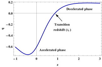
Figure 1: Behavior of the deceleration parameter vs redshift.

The behavior of the deceleration parameter $q$ versus $z$ corresponding to the values of the parameters constrained by the OHD+SNeIa datasets is displayed in Fig. 1. It can be seen that $q$ changes from negative to positive values at the value of the transition redshift $z_{t}=0.87$ with the current value of $q$ for our model is $q_{0}=-0.611$. Thus, the proposed model represents the transition of the Universe from the early deceleration phase to the current acceleration phase as shown by recent observations data (Planck 2020). Further, it is good to expand on the discussion of more geometrical parameters of the DE models to provide essential information about the evolution of our Universe. In the Taylor series expansion of the scale factor of the Universe with regard to cosmic time, there come the derivatives in the highest order of the deceleration parameter, which is famous as a jerk ($j$), snap ($s$), lerk ($l$) parameters. It can be said that the jerk parameter represents the evolution of the deceleration parameter. As we know that we can constrain $q$ from the observations data, the jerk parameter is studied to predict the future of the Universe and to compare other DE models with the $\Lambda$CDM model in which the value of $j$ is one always. In addition, the jerk parameter along with higher derivatives such as snap and lerk parameters provide a helpful understanding of the emergence of sudden future singularities (Pan et al. 2018).

The jerk ($j$), snap ($s$) and lerk ($l$) parameters are defined as (Pan et al. 2018),

$$j\left(z\right)=\frac{1}{H^{3}}\frac{da^{\left(3\right)}}{a}=\left(1+z\right)\frac{dq}{dz}+q\left(1+2q\right),$$ (30)

$$s\left(z\right)=\frac{1}{H^{4}}\frac{da^{\left(4\right)}}{a}=-\left(1+z\right)\frac{dj}{dz}-j\left(2+3q\right),$$ (31)

$$l\left(z\right)=\frac{1}{H^{5}}\frac{da^{\left(5\right)}}{a}=-\left(1+z\right)\frac{ds}{dz}-s\left(3+4q\right).$$ (32)

From the considered $q$ in Eq. (26), the jerk, snap and lerk equations are given as,

$$j\left(z\right)=\frac{\begin{array}[]{c}2q_{0}^{2}\left(z^{2}+1\right)^{2}+q_{0}\left(z^{2}+1\right)\left(4q_{1}(z+1)z+z^{2}+1\right)+q_{1}(z+1)\left((2q_{1}+1)z^{3}+(2q_{1}-1)z^{2}+3z+1\right)\end{array}}{\left(z^{2}+1\right)^{2}},$$ (33)

$$s\left(z\right)=-\frac{\begin{array}[]{c}6q_{0}^{3}\left(z^{2}+1\right)^{3}+q_{0}^{2}\left(z^{2}+1\right)^{2}\times\left(18q_{1}z(z+1)+7\left(z^{2}+1\right)\right)\\ +q_{0}\left(z^{2}+1\right)\times\left(18q_{1}^{2}z^{2}(z+1)^{2}+7q_{1}\left(2z^{4}+z^{3}+3z^{2}+5z+1\right)+2\left(z^{2}+1\right)^{2}\right)\\ +q_{1}(z+1)\times\left(\left(6q_{1}^{2}+7q_{1}+2\right)z^{5}+2\left(6q_{1}^{2}-1\right)z^{4}+2\left(3q_{1}^{2}+7q_{1}+4\right)z^{3}+4(7q_{1}-3)z^{2}+(7q_{1}+6)z+6\right)\end{array}}{\left(z^{2}+1\right)^{3}},$$ (34)

and,

$$l\left(z\right)=\frac{\begin{array}[]{c}24q_{0}^{4}\left(z^{2}+1\right)^{4}+2q_{0}^{3}\left(z^{2}+1\right)^{3}\left(48q_{1}z(z+1)+23\left(z^{2}+1\right)\right)\\ +q_{0}^{2}\left(z^{2}+1\right)^{2}\times\left(144q_{1}^{2}z^{2}(z+1)^{2}+46q_{1}\left(3z^{4}+2z^{3}+4z^{2}+6z+1\right)+29\left(z^{2}+1\right)^{2}\right)\\ +2q_{0}\left(z^{2}+1\right)\times\left(\begin{array}[]{c}48q_{1}^{3}z^{3}(z+1)^{3}+23q_{1}^{2}z\left(3z^{3}-2z^{2}+7z+2\right)(z+1)^{2}\\ +q_{1}\left(29z^{6}+11z^{5}+76z^{4}+28z^{3}-z^{2}+105z+40\right)+3\left(z^{2}+1\right)^{3}\end{array}\right)\\ +q_{1}(z+1)\times\left(\begin{array}[]{c}24q_{1}^{3}(z+1)^{3}z^{4}+46q_{1}^{2}(z+1)^{2}\left(z^{3}-z^{2}+3z+1\right)z^{2}\\ +q_{1}\left(29z^{7}-7z^{6}+101z^{5}-23z^{4}-45z^{3}+223z^{2}+115z+7\right)\\ +6\left(z^{7}-z^{6}+5z^{5}-5z^{4}+15z^{3}-15z^{2}-5z+5\right)\end{array}\right)\end{array}}{\left(z^{2}+1\right)^{4}}.$$ (35)

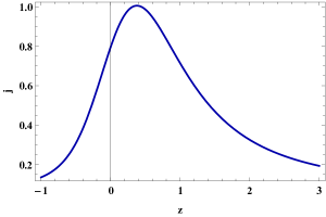
Figure 2: Behavior of the jerk parameter vs redshift.

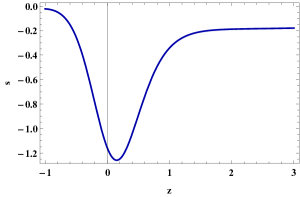
Figure 3: Behavior of the snap parameter vs redshift.

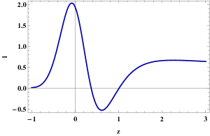
Figure 4: Behavior of the lerk parameter vs redshift.

From Figs. 2 and 4, it is clear that the current values of both parameters: jerk and lerk are positive (i.e. at redshift $z=0$) which represents an accelerated expansion of the Universe. Fig. 3 indicates the negative behavior of the snap parameter at present ($z=0$) that makes the Universe in an accelerating expansion currently. Also, the value of the current jerk parameter is not equal to one, which leads to our model not being similar to the behavior of the $\Lambda$CDM model at present (at $z=0$). Interestingly, this means that under certain modified gravity, late-time acceleration of the Universe can be seen using geometrical methods.

III.2 Om Diagnostic

With the development of modern cosmology and the emergence of many proposed models to solve the mystery of DE, it has become difficult to differentiate between these models. For this, an effective diagnostic parameter tool called $Om$ has been proposed in this context, extracted from the Hubble parameter (Sahni et al. 2008). This parameter easily tells us about the dynamical nature of DE models from the $Om(z)$ slope. The positive slope values of this diagnostic parameter tool indicate phantom nature ($\omega<-1$), while its negative values correspond to the quintessence nature ($\omega>-1$). The diagnostic $Om$ is defined as,

$$Om\left(z\right)=\frac{\left(\frac{H\left(z\right)}{H_{0}}\right)^{2}-1}{z^{3}+3z^{2}+3z}.$$ (36)

The diagnostic $Om$ for our current analysis is,

$$Om\left(z\right)=\frac{(z+1)^{2q_{0}+2}\left(z^{2}+1\right)^{q1}-1}{(z+1)^{3}-1}.$$ (37)

From Fig. 5 it is very clear that the positive slope value of $Om(z)$ indicates a quintessence-like behavior that represents the recently observed accelerating expansion of the Universe.

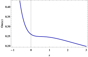
Figure 5: Behavior of the $Om\left(z\right)$ parameter vs redshift.

III.3 Cosmological Parameters

The evolution of the cosmic energy density, isotropic pressure, and EoS (Equation of State) parameter in terms of redshift are discussed below. Now, by using the values of $\rho$ and $p$ from (22) and (23) with the choice of $f\left(Q\right)$, we obtain the expression for cosmic energy density $\rho$ and isotropic pressure $p$ as follows:

$$\rho=\frac{\beta}{2}-\frac{\alpha}{2}6^{n+1}(2n+1)\left(H^{2}\right)^{n+1},$$ (38)

$$p=\frac{\alpha}{2}\left(-2^{n+1}\right)3^{n}(2n+1)\left(H^{2}\right)^{n+1}(2n(q+1)+2q-1)-\frac{\beta}{2}.$$ (39)

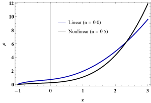
Figure 6: Behavior of the cosmic energy density vs redshift.

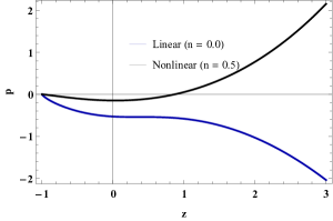
Figure 7: Behavior of the isotropic pressure vs redshift.

The plots in Figs. 6 and 7 exhibit very evident that the redshift evolution of cosmic energy density and isotropic pressure, derived here for the FLRW metric in the framework of $f(Q)$ gravity is fully consistent with the results derived in several works of literature (Shekh 2021, 2021a, 2022, Raja 2021). Specifically, the cosmic energy density is a positive and increasing function in terms of the redshift of both models (linear and nonlinear), while the isotropic pressure is negative in the present and the future. Thus, negative pressure is responsible for the acceleration phase of the Universe at the present.

The EoS parameter expression ($\omega=\frac{p}{\rho}$) for the cosmic fluid corresponding to the above cosmic energy density and isotropic pressure is,

$$\omega=\frac{\beta+\alpha 2^{n+1}3^{n}(2n+1)\left(H^{2}\right)^{n+1}(2n(q+1)+2q-1)}{\alpha 6^{n+1}(2n+1)\left(H^{2}\right)^{n+1}-\beta}.$$ (40)

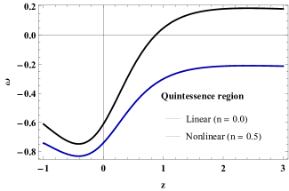
Figure 8: Behavior of the EoS parameter vs redshift.

In GR, an exotic form of energy (dark energy), described as negative isotropic pressure ($p<0$) or equivalently with a negative EoS parameter ($\omega<0$), has been proposed to be responsible for the accelerating expansion of the Universe. This last parameter relates to the cosmic energy density $\rho$ and isotropic pressure $p$ and describes the stages of the expansion of the Universe. It represents non-relativistic particles (matter) when $\omega=0$, and if $\omega=\frac{1}{3}$, this describes the relativistic particles (radiation) phase. The phantom region is represented by $\omega<-1$, while $-1<\omega\leq-\frac{1}{3}$ exhibits the quintessence region. Finally, for $\omega=-1$, the behavior of the $\Lambda$CDM model is shown. In general, for our model to predict the accelerating phase of the Universe, it must be $\omega\leq-\frac{1}{3}$. From Fig. 8, it is very clear that our model predicts accelerated expansion, and behaves like the quintessence model of dark energy in both models.

IV Energy Conditions

The so-called energy conditions (ECs) play an important role in the geodesics description of the Universe, and can be obtained from the the famous Raychaudhuri equation (Raychaudhuri 1955). In addition, ECs can be used to predict an accelerating Universe by violating the strong energy condition (SEC). If we consider that the content of the Universe is an perfect fluid, the ECs in $f(Q)$ gravity are

• Weak energy condition (WEC): $\rho+p\geq 0$ and $\rho\geq 0$;

• Null energy condition (NEC): $\rho+p\geq 0$;

• Dominant energy condition (DEC): $\rho\geq\left|p\right|$ and $\rho\geq 0$;

• Strong energy condition (SEC): $\rho+3p-6\overset{.}{f}_{Q}H+f\geq 0$

Taking Eqs. (38) and (39) into WEC, NEC, DEC and SEC conditions, we get

$$\text{WEC}\Leftrightarrow\rho+p=\alpha\left(-2^{n+1}\right)3^{n}\left(2n^{2}+3n+1\right)(q+1)\left(H^{2}\right)^{n+1}\geq 0\text{ and }\rho=\frac{\beta}{2}-\frac{\alpha}{2}6^{n+1}(2n+1)\left(H^{2}\right)^{n+1}\geq 0,$$ (41)

$$\text{NEC}\Leftrightarrow\rho+p=\alpha\left(-2^{n+1}\right)3^{n}\left(2n^{2}+3n+1\right)(q+1)\left(H^{2}\right)^{n+1}\geq 0,$$ (42)

$$\text{DEC}\Leftrightarrow\rho-p=\beta+\alpha 2^{n+1}3^{n}(2n+1)\left(H^{2}\right)^{n+1}(nq+n+q-2)\text{ and }\rho=\frac{\beta}{2}-\frac{\alpha}{2}6^{n+1}(2n+1)\left(H^{2}\right)^{n+1}\geq 0,$$ (43)

$$\text{SEC}\Leftrightarrow\rho+3p-6\overset{.}{f}_{Q}H+f=\alpha\left(-6^{n+1}\right)(n+1)(q-1)\left(H^{2}\right)^{n+1}\geq 0.$$ (44)

From Fig. 6 it is clear that the WEC condition (energy density) exhibits positive behavior. In addition, from Figs. 9, 10 and 11 we found that NEC and DEC conditions are satisfied, while the SEC condition is violated. As we said, violation of SEC condition leads to an acceleration phase of the Universe. The results obtained in our cosmological model are consistent with many papers in the literature.

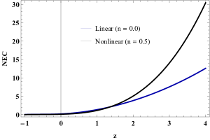
Figure 9: Behavior of the NEC condition vs redshift.

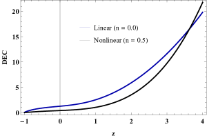
Figure 10: Behavior of the DEC condition vs redshift.

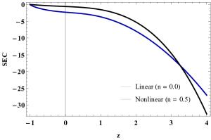
Figure 11: Behavior of the SEC condition vs redshift.

V Conclusion

The problem of the accelerating expansion of the Universe is one of the greatest mysteries of modern cosmology present time. Despite the most accepted $\Lambda$CDM model today can provide a significant match between theoretical predictions and observations, it however, lacks a convincing interpretation of the nature of dark energy (DE) described by the cosmological constant. This mystery motivated us in this work to suggest a simple cosmological model for dark energy within the framework of modified gravity theories such as $f\left(Q\right)$ symmetric teleparallel gravity, which describes the gravitational effects with a geometrical quantity called the non-metricity scalar $Q$. We considered two models to discuss the results, the linear and nonlinear model by assuming the function $f\left(Q\right)$ as $f(Q)=\alpha Q^{n+1}+\beta$, where $\alpha$, $\beta$ and $n$ are free model parameters. Also, it is important to mention that $n=0$ corresponds to $f(Q)=\alpha Q+\beta$ (linear model), while $n\neq 0$ corresponds to a case of the nonlinear model. We discussed some cosmographic parameters such as the jerk, snap and lerk parameters by assuming the divergence free parametric form of the deceleration parameter which gave a behavior consistent with the observations. Then, we obtained the expressions for cosmic energy density, isotropic pressure and EoS parameter for our cosmological model. We found that for both models specifically $n=0$ (linear model) and $n=0.5$ (nonlinear model), the cosmic energy density is a positive and increasing function in terms of the redshift, while the isotropic pressure is negative in the present and the future. To find out the dynamical nature of the model, we have discussed the $Om$ diagnostic and find a negative slope of the latter indicating quintessence-like behavior. Further, by analyzing the behavior of the EoS parameter, we found that one can get the quintessence model like behavior without introducing any DE component or exotic fluid into the matter part. Thus, in our analysis cosmic acceleration can only be explained by a geometrical generalization of general relativity. Finally, we discussed all the energy conditions (WEC, NEC, DEC and SEC) which were all fulfilled except for the SEC condition which was violated and this is fine in the course of our analysis. This work powerfully motivates us to look more at the new $f\left(Q\right)$ symmetric teleparallel gravity.

Data availability There are no new data associated with this article.

Declaration of competing interest The authors declare that they have no known competing financial interests or personal relationships that could have appeared to influence the work reported in this paper.

References

- [1] A.G. Riess et al., Astron. J. 116, 1009 (1998).
- [2] S. Perlmutter et al., Astrophys. J. 517, 565 (1999).
- [3] R.R. Caldwell, M. Doran, Phys. Rev. D 69, 103517 (2004).
- [4] Z.Y. Huang et al., JCAP 0605, 013 (2006).
- [5] C.L. Bennett et al., Astrophys. J. Suppl. 148, 119-134 (2003).
- [6] D.N. Spergel et al., [WMAP Collaboration], Astrophys. J. Suppl. 148, 175 (2003).
- [7] T. Koivisto, D.F. Mota, Phys. Rev. D 73, 083502 (2006).
- [8] S.F. Daniel, Phys. Rev. D 77, 103513 (2008).
- [9] D.J. Eisenstein et al., Astrophys. J. 633, 560 (2005).
- [10] W.J. Percival at el., Mon. Not. R. Astron. Soc. 401, 2148 (2010).
- [11] S.Weinberg, Rev. Mod. Phys. 61, 1 (1989).
- [12] B. Ratra and P.J.E. Peebles, Phys. Rev. D 37, 3406 (1998).
- [13] L. Xu et al., Phys. Rev. D 84, 123004 (2011).
- [14] R.R. Caldwell and M. Kamionkowski, and N.N. Weinberg, Phys. Rev. Lett. 91, 071301 (2003).
- [15] J.D. Barrow, Class. Quant. Grav. 21, L79 (2004).
- [16] J. B. Jimenez et al., Phys. Rev. D 98, 044048 (2018).
- [17] J. B. Jimenez et al., Phys. Rev. D 101, 103507 (2020).
- [18] Y. Xu et al., Eur. Phys. J. C 79, 8 (2019).
- [19] A. A. Starobinsky, Pisma Zh. Eksp. Teor. Fiz. 30, 719 (1979).
- [20] G.Bengochea, R. Ferraro, Phys. Rev. D 79, 124019 (2009).
- [21] S. Mandal, P.K. Sahoo and J.R.L. Santos, Phys. Rev. D 102, 024057 (2020).
- [22] D. Zhao, arXiv, arXiv:2104.02483.
- [23] S. Mandal et al., Phys. Rev. D 102, 124029 (2020).
- [24] N. Frusciante, Phys. Rev. D 103, 0444021 (2021).
- [25] M. Koussour et al. Phys. Dark Universe 36, 101051 (2022).
- [26] M. Koussour and M. Bennai Chin. J. Phys. (2022) doi: 10.1016/j.cjph.2022.09.002.
- [27] M. Koussour et al. Phys. Ann. Phys. 445, 169092 (2022).
- [28] T. Ortin, Gravity and Strings, Cambridge Monographs on Mathematical Physics (Cambridge University Press (2015).
- [29] M. Adak et al., Int. J. Mod. Phys. A 28, 1350167 (2013).
- [30] M. Adak, M. Kalay, and O. Sert, Int. J. Mod. Phys. D 15, 619 (2006).
- [31] I. Mol, Adv. Appl. Clifford Algebras 27, 2607 (2017).
- [32] R. Lazkoz et al., Phys. Rev. D 100, 104027 (2019).
- [33] T. Harko et al., Phys. Rev. D 98, 084043 (2018).
- [34] S. Capozziello and R. D’Agostino, Phys. Lett. B 832, 137229 (2022).
- [35] A.A. Mamon, S. Das, Int. J. Mod. Phys. D 25, 1650032 (2016).
- [36] W. El Hanafy, and G. G. L. Nashed, Phys. Rev. D 100, 083535 (2019).
- [37] G. N. Gadbail et al., Chin. J. Phys. 79, 246-255 (2022).
- [38] E. M. Barboza and J. S. Alcaniz, Phys. Lett. B 666, 415 (2008).
- [39] Planck Collaboration, Astron. Astrophys. 641, A6 (2020).
- [40] S. Pan, A.Mukherjee, N.Banerjee, Mon. Not. R. Astron. Soc. 477, 1 (2018).
- [41] V. Sahni, A. Shafieloo, and A. A. Starobinsky, Phys. Rev. D 78, 103502 (2008).
- [42] S. H. Shekh, Phys. Dark Universe 33 100850 (2021).
- [43] M. Koussour et al., Nucl. Phys. B. 978 115738 (2022).
- [44] S. H. Shekh et al., Universe 7, 3 (2021).
- [45] R. Solanki et al., Phys. Dark Universe 36, 100996 (2021).
- [46] A. Raychaudhuri, Phys. Rev. 98, 1123 (1955).