Hierarchical Cyclic Pursuit: Algebraic Curves Containing the Laplacian Spectra

Abstract

The paper addresses the problem of multi-agent communication in networks with regular directed ring structure. These can be viewed as hierarchical extensions of the classical cyclic pursuit topology. We show that the spectra of the corresponding Laplacian matrices allow exact localization on the complex plane. Furthermore, we derive a general form of the characteristic polynomial of such matrices, analyze the algebraic curves its roots belong to, and propose a way to obtain their closed-form equations. In combination with frequency domain consensus criteria for high-order SISO linear agents, these curves enable one to analyze the feasibility of consensus in networks with varying number of agents.

Cyclic pursuit, hierarchy, Laplacian spectra of digraphs, algebraic curves

1 Introduction

The Laplacian spectra of graphs play an important role in solving distributed optimization and control problems, since they mainly determine the stability and the convergence rate of the corresponding dynamical systems [1, 2, 3] For a fixed graph, finding the spectrum does not cause any difficulties, but if we consider graphs with a scalable structure (i.e., those constructed by the repetition of the same component), the problem of exact calculation or localization of the spectrum turns out to be non-trivial. A huge amount of literature is devoted to the derivation of formulas for the Laplacian spectra of undirected topologies, including various lattices such as rectangular grids, honeycombs (see [4] and the references therein), hierarchical small-world networks [5], products and coronas of graphs [6], and many others.

However, when analyzing the dynamics of network systems, directed communication topologies are of major interest. Say, it can be observed that a group of high-order agents may converge to consensus under an undirected interaction topology, however, it fails to do so under the corresponding uni-directed one, even though this topology contains a spanning converging tree. A precise localization of the Laplacian spectra of digraphs serves as the basis for the analysis of consensus problems in such situations.

In this paper, we study several generalizations of the cyclic pursuit multi-agent strategy. Its history can be traced back to 1878, when J.G. Darboux published his elegant work [7], where he studied some geometric averaging procedure and proved its convergence to consensus. Basically, cyclic pursuit is a strategy where agent $i$ pursues its neighbor $i-1$ modulo $N$, where $N$ is the number of agents. Evidently, such a communication structure is a uni-directed ring or a “predecessor–follower” topology, i.e., a Hamiltonian cycle.

Cyclic pursuit strategies attracted the attention of different scientific communities (see, e.g., [8, 9, 10, 11, 12, 13] and references therein) due to a wide range of applications including but not limited to numerous formation control tasks such as patrolling, boundary mapping, etc. Their extensions to hierarchical structures were considered in [14, 15, 16, 17]; papers [18], [19] addressed the case of heterogeneous agents; the effect of communication delays was analyzed in [20]; geometrical problems related to cyclic pursuit-like algorithms were studied in [21] and [22]. Some pursuit algorithms use the rotation operator in order to follow desired trajectories, see [23] and the references therein. The paper [24] shows the connection of discrete-time weighted cyclic pursuit with the general DeGroot model. Another group of strategies (protocols) is based on bi-directional topologies[25], that is, each agent $i$ has a relative information about its neighbors $i-1$ and $i+1$ (modulo $N$). The row straightening problems studied in[26, 27, 28] also imply symmetric communications except for fixed “anchors” (the endpoints of a segment). The problems of vehicle platooning with cyclic communications (see, e.g., [29, 30, 31, 32]) are also closely related to the problems of cyclic pursuit. In this case, the network system also has inputs including the desired inter-vehicular distances and communication disturbances. The analysis of the closed-loop stability of such systems is reduced to the study of state matrices close or identical to those studied in cyclic pursuit.

Regular ring structures model symmetric hierarchical interaction between agents. In some cases, these structures allow for closed-form expressions for the spectra of the corresponding Laplacian matrices, which helps to analyse the control protocols these matrices are involved in.

While cyclic pursuit can be treated as a special case of consensus seeking, the properties of the underlying interaction topology are closely related to classical mathematical considerations including the study of algebraic curves. For the basic cyclic pursuit topology, the eigenvalues of the corresponding Laplacian matrix are roots of unity [14]: no matter how many agents/nodes constitute the network, the spectrum lies on the unit circle. This fact prompted us to study hierarchical and other generalized ring topologies, which led to higher-order curves that contain their Laplacian spectra.

In this paper, we study ring digraphs with a hierarchical “necklace” structure. It is convenient to explore the Laplacian spectra of such graphs with regularly interleaved directed and undirected arcs using the concept of hierarchy. Namely, we introduce a macro-vertex, which is a sequence of directed and undirected arcs (the lower level of the hierarchy) and a directed ring of macro-vertices (the upper level of the hierarchy). The topologies constructed in this way occupy an intermediate position between directed and undirected rings, which have been widely studied in relation to cyclic pursuit and control of homogeneous vehicular platoons running on a ring (see, e.g., the nearest neighbor ring topologies presented in Fig. 2 (h) and (i) in [30]).

A useful classification of consensus problems based on the notion of complexity space was proposed in [33, Fig. 1.1]. In accordance with it, three independent dimensions of complexity can be identified in which the simplest first-order consensus model can be generalized, namely, (1) the complexity of the agent model, (2) topological complexity (complexity of the structure of interactions), and (3) the complexity of couplings between agents. The contribution of our paper to the general study of consensus in network systems can be attributed to the first two directions: the analysis and localization of the Laplacian spectra of special ring topologies to (2) and complex high-order models of agents to (1). Specifically, we prove that the Laplacian spectra of the studied digraphs lie on certain high-order algebraic curves irrespective of the number of macro-vertices forming the network. Along with this, we present an algorithm for obtaining equations of these curves. Based on this localization, we propose a geometric consensus condition in the frequency domain applicable to any number of interacting agents.

The paper is organized as follows. Section 2 introduces some mathematical preliminaries needed for the subsequent analysis and discusses the statement of the problem. The main results that describe the Laplacian spectra of ring digraphs are presented in Section 3. We prove that, regardless of the number of macro-vertices in such a digraph, its Laplacian spectrum lies on a certain algebraic curve and provide an algorithm to derive an implicit equation (of the form $p(x,y)=0$) of this curve in ${\mathbb{R}}^{2}$. In Section 4, we study consensus problems for a group of high-order linear SISO agents interacting through the discussed ring topologies, that is, performing hierarchical cyclic pursuit. We apply the frequency domain criterion [35, 36, 34] to derive a necessary and sufficient consensus condition, which does not depend on the number of agents in the network. The theoretical results are accompanied with numerical illustrations and, finally, conclusions are given.

Throughout the paper, $j\!:=\!\sqrt{-1}$ denotes the imaginary unit, while letters $i$ and $k$ are used for indexing purposes.

2 Preliminaries and Problem Statement

In this paper, we study network systems that have hierarchical ring structure. After defining the basic terminology, we formulate the problem.

Throughout the paper, we consider finite digraphs allowing in some cases multiple arcs and loops. A digraph is denoted by $\mathcal{G}_{N}=(\mathcal{V},\mathcal{E})$, where $\mathcal{V}=\{1,\ldots,N\}$ stands for the node set and $\mathcal{E}$ for the multiset of arcs.

The formal definitions of the adjacency and Laplacian matrices of an unweighted digraph $\mathcal{G}_{N}$ are given below.

Definition 1

The adjacency matrix associated with a digraph $\mathcal{G}_{N}=(\mathcal{V},\mathcal{E})$ is the matrix $\mathcal{A}_{N}=(a_{ik})\in{\mathbb{R}}^{N\times N}$, where each entry $a_{ik}$ is the number of arcs of the form $(i,k)$ in $\mathcal{E}.$

Definition 2

The Laplacian matrix $\mathcal{L}_{N}\in{\mathbb{R}}^{N\times N}$ of $\mathcal{G}_{N}$ is the matrix with entries $l_{ii}=\sum_{{\color[rgb]{0,0,0}k\neq i}}a_{ik}$ and $l_{ik}=-a_{ik}$ for $i\neq k,$ where $(a_{ik})=\mathcal{A}_{N}$ is the adjacency matrix of $\mathcal{G}_{N}$.

For example, consider a graph that represents communications within the conventional cyclic pursuit strategy for four agents (Fig. 1(a)). Here, an arc from $i$ to $k$ shows that agent $i$ pursues agent $k.$

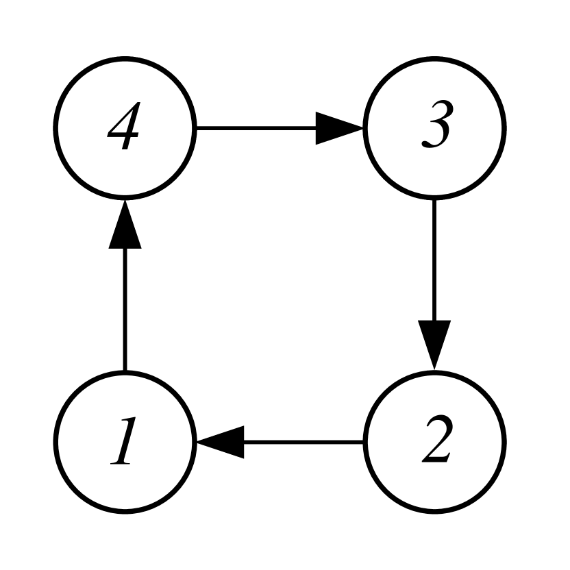
(a) The Hamiltonian cycle on 4 nodes

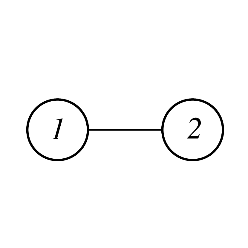
(b) A macro-vertex on 2 nodes

Figure 1: A Hamiltonian cycle corresponding to the cyclic pursuit strategy with four agents (a) and a macro-vertex (b)

The corresponding Laplacian matrix for the general case of $N$ agents can be defined through the counter-clockwise principal circulant permutation matrix [39] $\mathcal{P}_{N}$ as follows:

$$\mathcal{L}_{N}=I_{N}-\mathcal{P}_{N},$$

where $I_{N}\in\mathbb{R}^{N\times N}$ is the identity matrix,

$$\mathcal{P}_{N}=\begin{bmatrix}[r]0&0&0&\cdots&1\\ 1&0&0&\cdots&0\\ 0&1&0&\cdots&0\\ \vdots&\vdots&\ddots&\ddots&\vdots\\ 0&\cdots&0&1&0\end{bmatrix},$$ (1)

and

$$\mathcal{L}_{N}=\begin{bmatrix}[r]1&0&0&\cdots&-1\\ -1&1&0&\cdots&0\\ 0&-1&1&\cdots&0\\ \vdots&\vdots&\ddots&\ddots&\vdots\\ 0&\cdots&0&-1&1\end{bmatrix}.$$ (2)

We now describe the structure of hierarchical network systems studied below. The lower level of the hierarchy is a linear macro-vertex, which is a specific subdigraph whose $n\geq 1$ nodes are identified with indexed dynamical agents, while the top level is a Hamiltonian cycle on $m\geq 1$ macro-vertices.

Definition 3

A linear macro-vertex $\mathcal{G}^{i}_{n}=(\mathcal{V}^{i},\mathcal{E}^{i})$ of a digraph $\mathcal{G}_{N}=(\mathcal{V},\mathcal{E})$ is a subdigraph of $\mathcal{G}_{N}$ with $\mathcal{V}^{i}=\{v^{i}_{1},\ldots,v^{i}_{n}\}$ ($n\geq 1$) obtained from the directed path $v^{i}_{n}\to v^{i}_{n-1}\to\cdots\to v^{i}_{1}$ (main direction; no arcs when $n=1$) by adding the reverse path $v^{i}_{1}\to v^{i}_{2}\to\cdots\to v^{i}_{n}$ from which any subset of arcs is dropped.

The following definition introduces a topology consisting of $m$ identical macro-vertices on disjoint subsets of nodes along with a top-level Hamiltonian cycle that forms a Hamiltonian cycle on the whole set of $N=mn$ nodes together with the main direction paths traversing the macro-vertices. We will associate the term ring digraph with such a topology.

Definition 4

A ring digraph denoted by $\mathcal{G}_{m,n}=(\mathcal{V},\mathcal{E})$ is a digraph such that $\mathcal{V}=\bigcup_{i=1}^{m}\mathcal{V}^{i}$, $\mathcal{V}^{i}=\{n(i-1)+1,\ldots,ni\},$ $\mathcal{E}=\big{(}\bigcup_{i=1}^{m}\mathcal{E}^{i}\big{)}\cup\{e_{1},\ldots,e_{m}\},$ $(\mathcal{V}^{i},\mathcal{E}^{i})=\mathcal{G}^{i}_{n}$ are identical linear macro-vertices on $n\geq 1$ nodes, and the arcs $e_{i}=(ni+1,ni)$ $(i\in{\color[rgb]{0,0,0}\{1,\ldots,m-1\}})$ and $e_{m}=(1,nm)$ link the first node of each macro-vertex with the $n$th node of the previous one (which is the same macro-vertex when $m=1$).

It can be observed that each macro-vertex of a ring digraph is its induced subdigraph whenever $m>1$, while for $m=1$, it drops the arc $(1,n).$ The arcs $e_{1},\ldots,e_{m}$ form a Hamiltonian cycle on $m$ macro-vertices.

An example of a ring digraph with $n=2$ and $m=4$ is presented in Fig. 2. It is constructed from the Hamiltonian cycle shown in Fig. 1(a) and the macro-vertex (it is the complete digraph on two nodes) shown in Fig. 1(b), where a pair of opposite arcs is represented by a line segment without arrows.

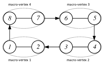
Figure 2: A ring digraph with four macro-vertices

Remark 1

A ring digraph can be considered as a Hamiltonian cycle $\{(1,N),(N,N-1),\ldots,(2,1)\}$ supplemented by the path $\{(1,2),(2,3),\ldots,{\color[rgb]{0,0,0}(N-1,N)}\}$ in which $\nu$ $({\color[rgb]{0,0,0}0\leq\nu\leq N-1})$ arcs are dropped in a regular fashion. In a sense, ring digraphs fill the gap between Hamiltonian cycle and bi-directional ring. Obviously, every ring digraph contains a spanning converging tree. It should be noted that this condition is necessary and sufficient for attaining asymptotic consensus in the system consisting of first-order agents. In Section 4, we consider a more general setting with high-order agent models and derive a consensus condition that does not depend on the number of nodes in the network.

We now introduce cooperating agents and then formulate the problem. The agents are assumed to have identical high-order (double integrator or higher) SISO linear models. Let $x_{i}\in\mathbb{R}$ represent the position of agent $i$, $i\in\{1,\ldots,N\}$. Therefore, the consensus-seeking communication over the network $\mathcal{G}_{m,n}$ can be described as

$${\rm\bf a}(s)x_{i}=u_{i},$$ (3)

$$u_{i}={\rm\bf b}(s)\left(\sum_{k\in\mathcal{N}_{i}}a_{ik}(x_{k}-x_{i})\right),\quad i\in{\color[rgb]{0,0,0}\{1,\ldots,N\}}{\color[rgb]{0,0,0},}$$ (4)

where $a_{ik}$ are the elements of the adjacency matrix $\mathcal{A}_{N}$ and $\mathcal{N}_{i}$ is the set of neighbors of node $i,$ i.e., the set of nodes $k$ such that $a_{ik}\neq 0$. Here $s:=\frac{d}{dt}$ denotes the differentiation operator, the scalar polynomials

$${\rm\bf a}(s)=s^{d}+{\rm\bf a}_{d-1}s^{d-1}+\ldots+{\rm\bf a}_{1}s+{\rm\bf a}_{0},$$

$${\rm\bf b}(s)={\rm\bf b}_{q}s^{q}+{\rm\bf b}_{q-1}s^{q-1}+\ldots+{\rm\bf b}_{1}s+{\rm\bf b}_{0}$$

determine agent’s dynamics and communications, and $u_{i}$ is the control signal. For convenience, we assume $d>q$.

Let us introduce the vector $\xi_{i}=[x_{i},~{}\dot{x}_{i},\ldots,x^{(d-1)}_{i}]^{\top}$ and transform equations (3), (4) into the state-space form

$$\dot{\xi}_{i} = A\xi_{i}+Bu_{i},$$ (5)

$$u_{i} = K\sum_{k\in\mathcal{N}_{i}}a_{ik}(\xi_{k}-\xi_{i}),\quad i\in{\color[rgb]{0,0,0}\{1,\ldots,N\}},$$ (6)

where

$$A=\begin{bmatrix}[r]0&1&0&\cdots&0\\ 0&0&1&\cdots&0\\ 0&0&0&\cdots&0\\ \vdots&\vdots&\vdots&\cdots&\vdots\\ 0&0&0&\cdots&1\\ -{\rm\bf a}_{0}&-{\rm\bf a}_{1}&-{\rm\bf a}_{2}&\cdots&-{\rm\bf a}_{d-1}\end{bmatrix},\quad B=\begin{bmatrix}[r]0\\ 0\\ 0\\ \vdots\\ 0\\ 1\end{bmatrix},$$

$$K=\begin{bmatrix}[r]{\rm\bf b}_{0}&{\rm\bf b}_{1}&{\rm\bf b}_{2}&\ldots&{\rm\bf b}_{q}&0&\ldots&0\end{bmatrix}.$$

The entire closed-loop dynamics can thus be written as

$$\dot{\xi}=({I}_{N}\otimes A-\mathcal{L}_{N}\otimes{BK})\xi,$$ (7)

where $\xi=[\xi^{\top}_{1},~{}\xi^{\top}_{2},\ldots,\xi^{\top}_{N}]^{\top}$ and $\otimes$ is the Kronecker product.

In Section 4, we will obtain a consensus criterion for ring-shaped networks of agents (3), (4).

Let us formulate a definition of consensus for the systems under study.

Definition 5

We say that the network system (5) with feedback control (6) reaches consensus if

$$\lim_{t\to\infty}{\|\xi_{i}(t)-\xi_{k}(t)\|}=0,\quad\forall i,k\in{\color[rgb]{0,0,0}\{1,\ldots,N\}}$$ (8)

for any initial condition $\xi(0)=[\xi_{1}^{\top}(0),\ldots,\xi_{N}^{\top}(0)]^{\top}$.

In the simplest case of ${\rm\bf a}(s)=s$ and ${\rm\bf b}(s)=1$ we face the classical first-order consensus model; e.g., the cyclic pursuit if $a_{ik}=1$ for $k=i-1\pmod{N}$ and $a_{ik}=0$ otherwise. The corresponding Laplacian matrix $\mathcal{L}_{N}$ is given by (2), and its characteristic polynomial $\Delta(\lambda)$ has the form

$$\Delta(\lambda)=(\lambda-1)^{N}-1.$$

The roots of $\Delta(\lambda)$ can be found using Lemma 1, which follows from De Moivre’s Theorem.

Lemma 1

The roots of the cyclotomic equation

$$\sigma^{N}-1=0$$ (9)

are

$$\sigma_{k}={\rm e}^{j\frac{2\pi k}{N}},\;k\in{\color[rgb]{0,0,0}\{0,\ldots,N-1\}},$$ (10)

and the roots of

$$\sigma^{N}+1=0$$ (11)

are

$$\sigma_{k}={\rm e}^{j\frac{2\pi k+\pi}{N}},\;k\in{\color[rgb]{0,0,0}\{0,\ldots,N-1\}}.$$ (12)

The roots in both sets are uniformly distributed on the unit circle centered at $(0,~{}j0)$ in the complex plane ${\mathbb{C}}$.

Therefore, the spectra of the Laplacian matrices (2) with all $N\in{\mathbb{N}}$ are jointly dense on the unit circle centered at $(1,~{}j0)$.

The equation of the corresponding unit circle in $\mathbb{R}^{2}$ is

$$(x-1)^{2}+y^{2}-1=0.$$ (13)

This circle is a basic example of a curve that contains the Laplacian spectrum of a ring digraph; it entirely lies in ${\mathbb{C}}^{+}\cup\{0\}.$ The spectrum of any such a digraph contains $0$ with multiplicity $1,$ which guarantees consensus in the first order cyclic pursuit process according to the well-known consensus criterion.

Remark 2

The dynamic system (3), (4) can be considered from different points of view: Its coordinates can have different physical meanings, and the signal $u_{i}$ can contain both the plant dynamics and elements of a local or/and a distributed controller. In addition, the right-hand side can also contain additional external signals and disturbances that do not affect the form of the state matrix of the closed loop system (7). A particular example of such a system is a leaderless vehicle platoon moving on a ring, see, e.g., [29, 30, 31, 32]. In such problems, two types of stability are studied: The classical stability of a closed loop system and string stability associated with the amplification of a disturbance propagating through the system (see [37], [38] and references therein). With an increase in the number of vehicles $N$ in the platoon, the system may exhibit eventual instability [37]. Therefore, the problem of stabilization regardless of the number $N$ is important.

The paper aims at:

• localizing the Laplacian spectra of the ring digraphs defined above;

• obtaining a necessary and sufficient consensus condition applicable to any number of agents in the network.

3 Laplacian Spectra of Ring Digraphs

In this section, we propose a method for exact localization of Laplacian spectra for ring digraphs. It turns out that these spectra always lie on algebraic curves whose expressions can be found in closed form. Thus, equations of these curves are among the main results of the work.

First, we classify ring digraphs and discuss their properties. After that we

• derive a general form of the characteristic polynomial of the corresponding Laplacian matrices;

• present a way to obtain the equations of algebraic curves that contain the roots of the characteristic polynomial regardless of the number of nodes in $\mathcal{G}_{m,n}$.

3.1 Simple and Complex Rings

Let us find out how the set of ring digraphs is organized. Clearly, different macro-vertices can give rise to isomorphic ring digraphs. For instance, consider the two macro-vertices depicted in Fig. 3a,b, where each macro-vertex has an unattached dotted arc of a Hamiltonian cycle connecting macro-vertices within a ring digraph. Obviously, two macro-vertices of type (a) form the same digraph (shown in Fig. 2) as four macro-vertices of type (b).

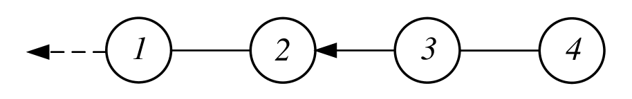
(a) A macro-vertex on 4 nodes

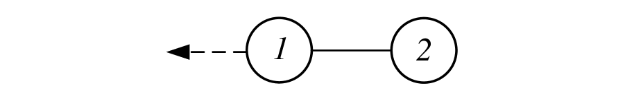
(b) A macro-vertex on 2 nodes

Figure 3: A macro-vertex (a) on four nodes can be obtained by connecting two macro-vertices of type (b) by a directed arc.

By construction, ring digraphs are scalable, i.e., they can be “inflated” by cloning macro-vertices. To distinguish the types of such digraphs and characterize their simplest components, we introduce the following definition.

Definition 6

A ring digraph will be called a complex ring if it can be represented as a Hamiltonian cycle on two or more macro-vertices. If this is not the case, we call it a simple ring. A complex ring $\mathcal{G}_{m,n}$ is said to be a round replication of a simple ring $\mathcal{G}_{1,n}$ if the representations of $\mathcal{G}_{m,n}$ and $\mathcal{G}_{1,n}$ involve identical macro-vertices.

While examples of simple and complex rings are shown in Fig. 4, the theorem below recursively counts the number of non-isomorphic simple rings with a given number of nodes.

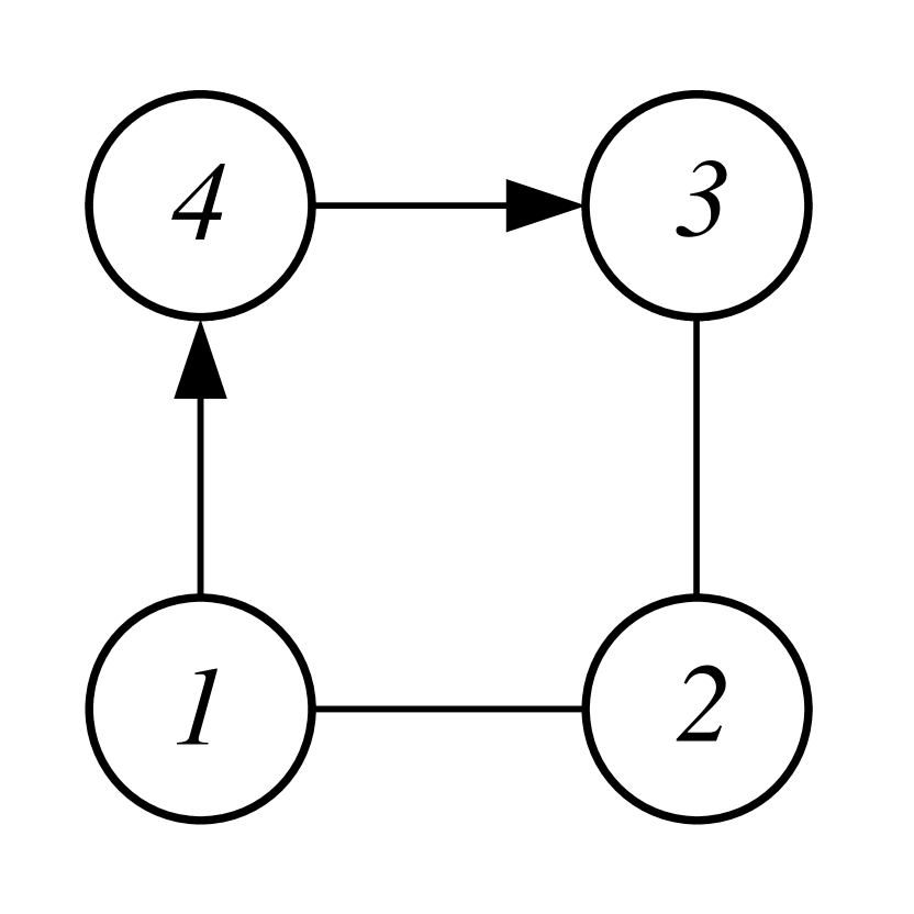
(a) A simple ring on 4 nodes

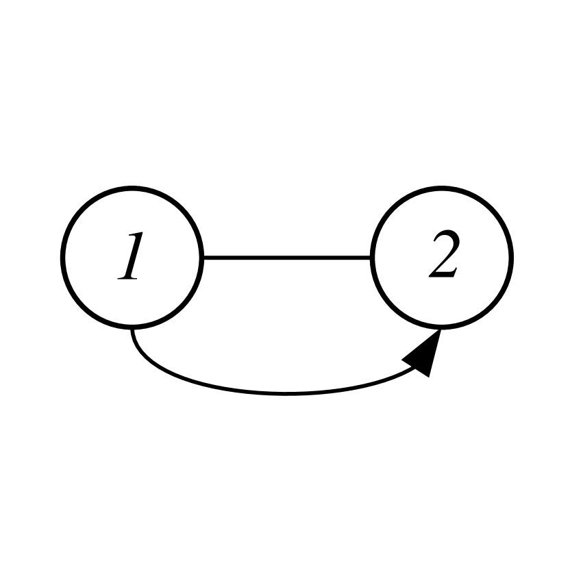
(b) A simple ring on 2 nodes

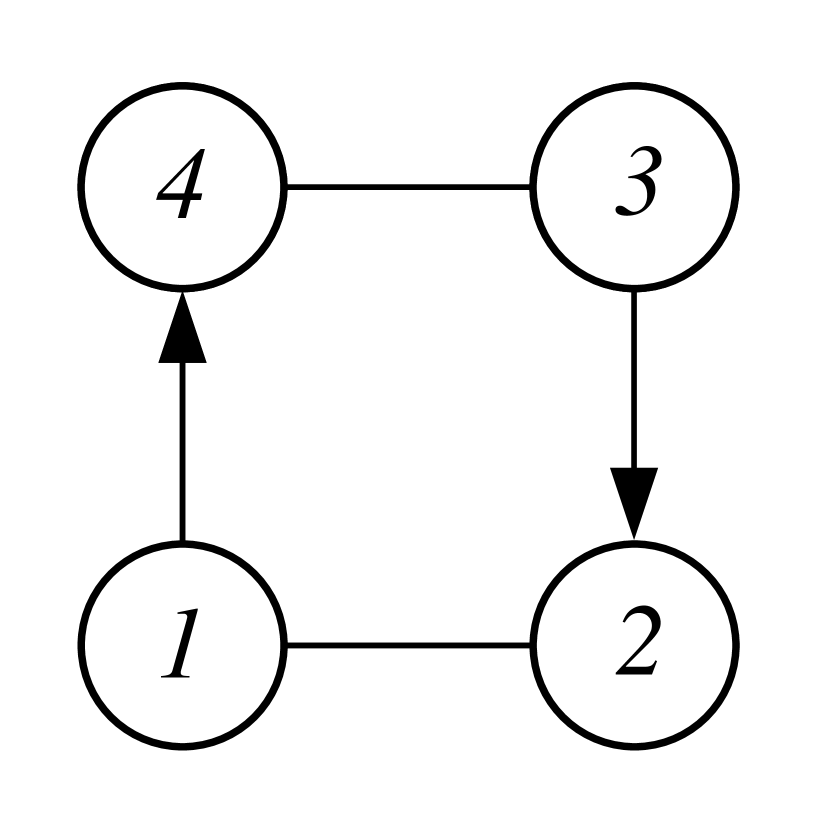
(c) A complex ring on 4 nodes

Figure 4: Two simple rings ((a) and (b)) and a complex ring (c) constructed as the round replication of the simple ring (b)

Theorem 1

The number $Y(N)$ of non-isomorphic simple rings on $N$ nodes satisfies the relationship

$$Y(N)=\frac{2^{N}-\mathop{\sum}\limits_{n\in D(N)}nY(n)}{N},$$ (14)

where $D(N)$ is the set of all divisors of $N$ excluding $N$ and $Y(1)$ is set to be $2.$

First, to simplify the proof, we redefine ring digraph on $N=1$ node (cyclic pursuit of a single agent makes no sense, so this redefinition does not affect the application) as a multidigraph that has either $1$ or $2$ directed loops. Then $Y(1)=2,$ as stated in Theorem 1. Next, for any $N>1$ let us supplement the set of ring digraphs on $N$ nodes with all digraphs of the same form that additionally have arc $(N,1),$ where $N=mn$ (this arc is absent in ring digraphs by definition). The supplemented set of ring digraphs will be called the set of necklace digraphs.

Any necklace digraph on the node set $\mathcal{V}=\{1,\ldots,N\}$ can be identified with a vector $(a_{1},\ldots,a_{N}),$ where $a_{i}=2$ if and only if there are two opposite arcs between nodes $i$ and $i+1\pmod{N}$ and $a_{i}=1$ otherwise.

A necklace digraph is periodic if its vector representation is periodic in the sense that $(a_{1},\ldots,a_{N})=(a_{1},\ldots,a_{n},a_{1},\ldots,a_{n},\ldots,a_{1},\ldots,a_{n})$ with $n<N$ being the minimum length of a subvector whose replication gives the whole vector.

Denote by ${\widetilde{Y}}(N)$ the number of non-isomorphic non-periodic necklace digraphs on $N$ nodes. Obviously, there is a bijection between such digraphs and distinct cycles of minimal period $N$ (in the case of two contractivity factors) enumerated in [42] (Lemma 1 in Section 4.8). Consequently, ${\widetilde{Y}}(N)=(2^{N}-\sum_{n\in D(N)}n{\widetilde{Y}}(n))/N.$

Finally, we prove that $Y(N)={\widetilde{Y}}(N)$ for all $N\in{\mathbb{N}}.$ We have $Y(1)={\widetilde{Y}}(1)$ by redefinition. For $N>1,$ consider any non-periodic necklace digraph. Its vector representation contains at least one $a_{i}=1.$ Therefore, it can be transformed into the representation of a simple ring by a number of cyclic shifts transferring $a_{i}=1$ to the position $a_{N}$ corresponding to the pair of nodes $(N,1).$ This defines a one-to-one correspondence between the equivalence classes of isomorphic non-periodic necklace digraphs and the classes of isomorphic simple rings (all on $N$ nodes). Hence, the number of the latter classes is given by (14). This completes the proof.

$N$	1	2	3	4	5	6	7	8	9	10	11	12	13	14	15	16	17	18	19	20
$Y(N)$	2	1	2	3	6	9	18	30	56	99	186	335	630	1161	2182	4080	7710	14532	27594	52377

Table 1: The first values of the function $Y(N)$, the number of non-isomorphic ring digraphs on $N$ nodes

Corollary 1

$1.$ If $N$ is prime, then $Y(N)=(2^{N}-2)/N.$
$2.$ If $N=2^{p},$ $p\in{\mathbb{N}},$ then $Y(N)=(2^{N}-2^{N/2})/N.$

The first statement is a direct consequence of Theorem 1. To prove the second one by induction, first observe that in the base case, $p=1,$ it follows from the first part. Assume that it is true for all $N=2^{k},$ $k<p$ and prove it for $N=2^{p}.$ In this case, $D(N)=\{1,2,\ldots,N/2\}.$ By Theorem 1 and the induction hypothesis, it holds that $Y(N)=(2^{N}-2^{1}-(2^{2}-2^{1})-\ldots-(2^{N/2}-2^{N/4}))/N=(2^{N}-2^{N/2})/N,$ as desired.

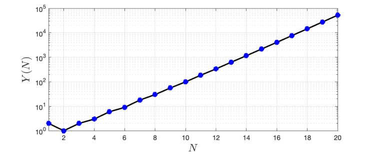
Figure 5: The quantity $Y(N)$ as function of the number of nodes

Some values of the function $Y(N)$ (modified for $N=1$) are given in Table 1. Figure 5 illustrates its growth graphically using base-10 logarithmic scale on the vertical axis.

Remark 3

In the proof of Theorem 1, we reduced the enumeration of non-isomorphic simple rings on $N$ nodes to that of distinct cycles of minimal period $N.$ Essentially the same numerical sequence appeared as a solution to a number of other equivalent enumeration problems including those of dimensions of the homogeneous parts of the free Lie algebras, irreducible polynomials of degree $N$ over the field GF$(2)$, binary Lyndon words of length $N$, etc. (see sequences A001037 and A059966 in [43]).

It is worth mentioning that expression (14) has significant consequences regarding the divisibility of numbers. Say, part 1 of Corollary 1 implies a special case of Fermat’s little theorem ($a^{p}\equiv a\pmod{p}$, where $p$ is prime) for $a=2,$ while extending (14) to multigraphs gives a proof of this theorem in its general form.

3.2 Laplacian Spectra and Algebraic Curves

We now consider complex rings with $N>3$ nodes and characterize the locus of the corresponding Laplacian spectra.

Theorem 2

For any simple ring $\mathcal{G}_{1,n}$ on $n$ nodes, the Laplacian eigenvalues of all complex rings $\mathcal{G}_{m,n}$ obtained by $m$-fold round replication of $\mathcal{G}_{1,n}$ belong to a bounded algebraic curve of order $2n$ in ${\mathbb{C}}^{+}\cup\{0\}.$

In accordance with Theorem 4 in [44], the Laplacian characteristic polynomial of $\mathcal{G}_{m,n}$ has the form

$$\Delta(\lambda)=(P_{n}(\lambda))^{m}-(-1)^{N},$$ (15)

where $P_{n}(\lambda)=\prod_{k=1}^{K}Z_{i_{k}}$ is an $n$th order polynomial and $i_{1},\ldots,i_{K}$ are the path lengths in the decomposition of the cycle $\{(1,n),(n,n-1),\ldots,(2,1)\}$ into the paths linking the consecutive nodes of indegree 1 in $\mathcal{G}_{1,n}$. The polynomials $Z_{i}$ are the modified Chebyshev polynomials of the second kind:

$$Z_{n}(\lambda):=(\lambda-2)Z_{n-1}(\lambda)-Z_{n-2}(\lambda),$$

where $Z_{0}(\lambda)\equiv 1$ and $Z_{1}(\lambda)\equiv\lambda-1$.

By Lemma 1, the roots $\alpha_{k}+j\beta_{k},$ $k\in\{0,\ldots,m-1\}$ of $\sigma^{m}-(-1)^{N}=0$ are roots of unity (the roots of $\sigma^{m}=-1$ are also roots of $\sigma^{2m}=1$) lying on the unit circle in ${\mathbb{C}}$. Therefore, by (15), the zeros of $\Delta(\lambda)$ satisfy

$$P_{n}(\lambda)=\alpha_{k}+j\beta_{k},\quad k\in{\color[rgb]{0,0,0}\{0,\ldots,m-1\}},$$ (16)

where

$$\alpha_{k}^{2}+\beta_{k}^{2}=1.$$ (17)

Varying $m$ we obtain a countable set of roots of unity, which is everywhere dense on the unit circle. This means that for any $u,v\in{\mathbb{R}}$ such that $u^{2}+v^{2}=1,$ there exist sequences $u_{i}\to u$ and $v_{i}\to v$ such that $u_{i}+jv_{i}$ are roots of unity $(i\in{\mathbb{N}}).$ Based on this we apply Theorem 11.1 in [45] on the continuous dependence of the roots of a polynomial with leading coefficient 1 on its other coefficients (cf. [46, 47]). Due to this theorem, if $\lambda_{k},$ $k\in\{0,\ldots,n-1\},$ are the roots of equation $P_{n}(\lambda)=u+jv,$ then the roots $\lambda_{k,i}$ of equations $P_{n}(\lambda)=u_{i}+jv_{i}$ $(k\in\{0,\ldots,n-1\},i\in{\mathbb{N}})$ can be numbered in such a way that $\lambda_{k,i}\to\lambda_{k},$ $k\in\{0,\ldots,n-1\}.$ This justifies the following method for determining the curve (in the implicit form $f(x,y)=0$) on which the Laplacian eigenvalues of complex rings $\mathcal{G}_{m,n}$ are everywhere dense. Setting $\lambda=x+jy$ for (16) and substituting ${\rm Re}[P_{n}(x+jy)]=\alpha_{k}$ and ${\rm Im}[P_{n}(x+jy)]=\beta_{k}$ into (17) yields an equation of order $2n,$ which determines the desired algebraic curve of order $2n$ in the form $f(x,y)=0.$ Indeed, this curve contains the roots of (16) for all $\alpha_{k}+j\beta_{k}$ that belong to the unit circle. According to the above continuity theorem, any neighborhood of each such a root contains infinitely many roots of (16) in which $\alpha_{k}+j\beta_{k}$ are roots of unity. The latter roots lie on the same curve and are the Laplacian eigenvalues of ring digraphs $\mathcal{G}_{m,n}.$

By the properties of the Laplacian spectra of digraphs, they lie in ${\mathbb{C}}^{+}\cup\{0\}$. Substituting $\lambda=|\lambda|(\cos\varphi+j\sin\varphi)$ into $P_{n}(\lambda)=\lambda^{n}+\sum_{k=0}^{n-1}p_{k}\lambda^{k}$ for $\lambda\neq 0$ we have $|P_{n}(\lambda)|=|\lambda|^{n}\,|1+\sum_{k=0}^{n-1}p_{k}\lambda^{-n+k}(\cos{k\varphi}+j\sin{k\varphi})|.$ Therefore, it is easy to specify $h>0$ such that $|\lambda|>h$ implies $|P_{n}(\lambda)|>1.$ Consequently, $\lambda$ with $|\lambda|>h$ cannot satisfy (16) and thus the Laplacian spectra locus of ring digraphs $\mathcal{G}_{m,n}$ is bounded. This completes the proof.

Let us emphasize that an unbounded “inflation” of a ring digraph $\mathcal{G}_{m,n}$ by increasing $m$ leaves the Laplacian eigenvalues on the same algebraic curve and only increases their density on it.

Corollary 2

For a fixed $n\in{\mathbb{N}}$, the number of distinct algebraic curves of order $2n$ containing the Laplacian spectra of ring digraphs obtained by round replication of simple rings on $n$ nodes does not exceed the number of non-isomorphic simple rings on $n$ nodes determined by Theorem 1.

3.3 Quartic and Sextic Curves

In this section, we consider several special cases that allow relatively simple closed-form expressions of the corresponding algebraic curves mentioned in Theorem 2.

The case $n=2$. We first consider a complex ring with the following structure: It has $N=2m$ nodes, $m\geq 2$, and contains a Hamiltonian cycle supplemented by the inverse cycle, where every second arc is dropped (Fig. 6). This digraph is a round replication of the simple ring depicted in Fig. 4(b); the ring digraph in Fig. 2 belongs to this class with $m=4.$

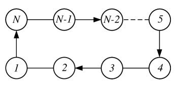
Figure 6: A round replication of the simple ring shown in Fig. 4(b)

The Laplacian matrix of this digraph has the form

$$\mathcal{L}_{N}=\begin{bmatrix}[r]2&-1&0&0&\cdots&0&-1\\ -1&1&0&0&\cdots&0&0\\ 0&-1&2&-1&\cdots&0&0\\ \vdots&\vdots&\ddots&\ddots&\ddots&\vdots&\vdots\\ 0&\cdots&0&-1&1&0&0\\ 0&\cdots&0&0&-1&2&-1\\ 0&\cdots&0&0&0&-1&1\end{bmatrix},$$ (18)

and by (15), its characteristic polynomial is $(Z_{2})^{\frac{N}{2}}-1$ $=(\lambda^{2}-3\lambda+1)^{m}-1$. Its roots satisfy

$$\lambda^{2}-3\lambda+1-\alpha_{k}-j\beta_{k}=0,\quad k\in\{0,\ldots,m-1\}.$$

From $(x+jy)^{2}-3(x+jy)+1-\alpha_{k}-j\beta_{k}=0$ it follows $\alpha_{k}=(x-1.5)^{2}-y^{2}-1.25$ and $\beta_{k}=2xy-3y$. Substituting the last expressions into formula (17) gives the equation of the curve.

In this case, the eigenvalues of the Laplacian matrix (18) lie on the quartic Cassini curve (Cassini ovals) defined by

$$[(\tilde{x}-\sqrt{5})^{2}+\tilde{y}^{2}][(\tilde{x}+\sqrt{5})^{2}+\tilde{y}^{2}]=2^{4},$$ (19)

where $\tilde{x}=2(x-3/2)$ and $\tilde{y}=2y$, see [48] for the details. This curve is shown in Fig. 7.

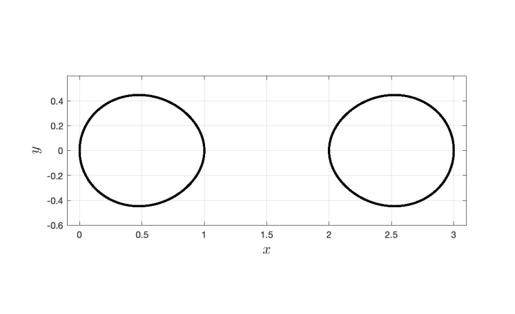
Figure 7: Cassini ovals

The case $n=3$. Observe that there are exactly two non-isomorphic simple rings on $n=3$ nodes; these are depicted in Fig. 8.

(a) Simple ring #1

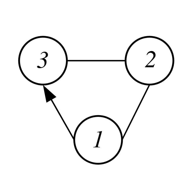
(b) Simple ring #2

Figure 8: Two simple rings on $n=3$ nodes

Consider two complex rings on $N=3m$ nodes ($m>1$) constructed by round replication of these simple rings. The one obtained from simple ring #1 is shown in Fig. 9.

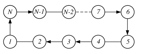
Figure 9: The ring digraph obtained by round replication of the simple ring in Fig. 8(a)

Its Laplacian matrix has the form

$$\mathcal{L}_{N}=\begin{bmatrix}[r]2&-1&0&0&\cdots&0&-1\\ -1&1&0&0&\cdots&0&0\\ 0&-1&1&0&\cdots&0&0\\ \vdots&\vdots&\ddots&\ddots&\ddots&\vdots&\vdots\\ 0&\cdots&0&-1&2&-1&0\\ 0&\cdots&0&0&-1&1&0\\ 0&\cdots&0&0&0&-1&1\end{bmatrix},$$ (20)

and by (15), its characteristic polynomial is $(Z_{1}Z_{2})^{\color[rgb]{0,0,0}m}-(-1)^{N}$.

According to Theorem 2, the eigenvalues of the matrix (20) lie on a sextic curve. Its equation is

$$(\tilde{x}^{2}+\tilde{y}^{2})^{3}+(4+4\tilde{x})(\tilde{x}^{2}+\tilde{y}^{2})^{2}-2\tilde{x}^{3}-4\tilde{x}^{2}$$ (21)

$$+\,6\tilde{x}\tilde{y}^{2}+4\tilde{y}^{2}=0,$$

where $\tilde{x}=x-2$ and $\tilde{y}=y$. This curve is depicted in Fig. 10.

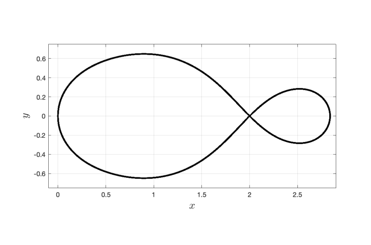
Figure 10: The sextic curve defined by (21)

The complex ring constructed by round replication of simple ring #2 (Fig. 8(b)) is shown in Fig. 11.

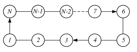
Figure 11: The ring digraph obtained by round replication of the simple ring in Fig. 8(b)

Its Laplacian matrix is of the form

$$\mathcal{L}_{N}=\begin{bmatrix}[r]2&-1&0&0&\cdots&0&-1\\ -1&2&-1&0&\cdots&0&0\\ 0&-1&1&0&\cdots&0&0\\ \vdots&\vdots&\ddots&\ddots&\ddots&\vdots&\vdots\\ 0&\cdots&0&-1&2&-1&0\\ 0&\cdots&0&0&-1&2&-1\\ 0&\cdots&0&0&0&-1&1\end{bmatrix};$$ (22)

and by (15), its characteristic polynomial is $(Z_{3})^{\color[rgb]{0,0,0}m}-(-1)^{N}$.

By Theorem 2, the eigenvalues of the matrix (22) lie on a sextic curve; it is defined by equation

$$(\tilde{x}^{2}+\tilde{y}^{2})^{3}+2\tilde{x}(\tilde{x}^{2}+\tilde{y}^{2})^{2}-3\tilde{x}^{4}-6\tilde{x}^{3}+2\tilde{x}^{2}\tilde{y}^{2}$$ (23)

$$+\,2\tilde{x}^{2}+2\tilde{x}\tilde{y}^{2}+4\tilde{x}+5\tilde{y}^{4}+6\tilde{y}^{2}=0,$$

where $\tilde{x}=x-2$ and $\tilde{y}=y$. This curve is depicted in Fig. 12.

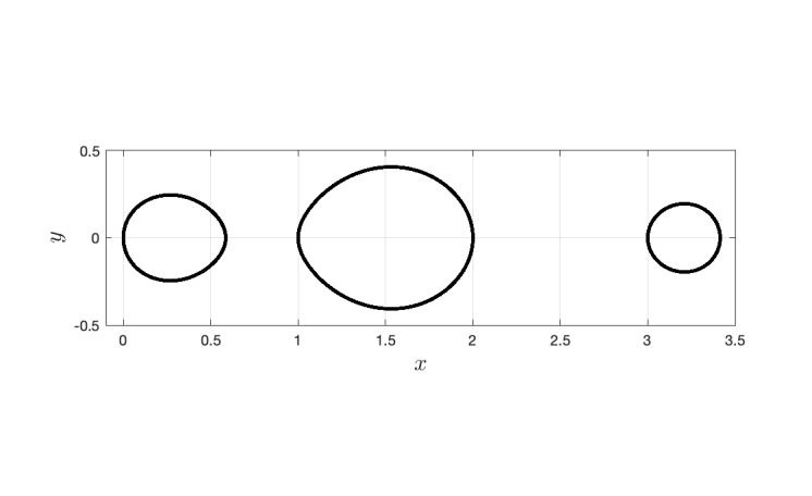
Figure 12: The sextic curve defined by (23)

Graphs with a more complex structure based on simple rings on $4,5,\ldots$ nodes can be obtained in the same way along with the corresponding expressions for higher-order curves that contain the spectrum loci.

In subsection 3.4, we present a result involving a weighted necklace digraph. Such a structure generalizes the topology of cyclic pursuit in a different way: There are no macro-vertices, but the arcs of one of the directions are weighted and have the same weight. Due to the presence of this variable weight, the corresponding Laplacian spectra belong to a certain drop-shaped region rather than lie on an algebraic curve.

3.4 A Weighted Ring

Consider a weighted necklace digraph on $N$ nodes consisting of a Hamiltonian cycle and the inverse one.

Assume that all arcs of one of the cycles have the same weight $a$, and the arcs in the opposite direction have weight $b$. Without loss of generality we can restrict ourselves to the case where one weight is unity and the other one is $c\in[0,~{}1]$.

A digraph of this type is shown in Fig. 13.

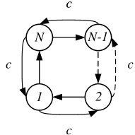
Figure 13: A two-cycle weighted digraph

Its Laplacian matrix has the form

$$\mathcal{L}_{N}=\begin{bmatrix}[r]\!1+c\!&\!-c\!&\!0\!&\!0\!&\!\cdots\!&\!0\!&\!-1\!\\ \!-1\!&\!1+c\!&\!-c\!&\!0\!&\!\cdots\!&\!0\!&\!0\!\\ \!0\!&\!-1\!&\!1+c\!&\!-c\!&\!\cdots\!&\!0\!&\!0\!\\ \!\vdots\!&\!\vdots\!&\!\ddots\!&\!\ddots\!&\!\ddots\!&\!\vdots\!&\!\vdots\!\\ \!0\!&\!\cdots\!&\!0\!&\!-1\!&\!1+c\!&\!-c\!&\!0\!\\ \!0\!&\!\cdots\!&\!0\!&\!0\!&\!-1\!&\!1+c\!&\!-c\!\\ \!-c\!&\!\cdots\!&\!0\!&\!0\!&\!0\!&\!-1\!&\!1+c\!\end{bmatrix}.$$ (24)

Lemma 2

For any weight $c\in[0,~{}1]$ and any $N\in{\mathbb{N}},$ the eigenvalues of matrix (24) lie on the ellipse

$$\frac{(x-(1+c))^{2}}{(1+c)^{2}}+\frac{y^{2}}{(1-c)^{2}}=1.$$ (25)

Obviously, $\mathcal{L}_{N}=(1+c)I_{N}-\mathcal{P}_{N}-c\mathcal{P}_{N}^{N-1}$, where $\mathcal{P}_{N}$ is the counter-clockwise principal circulant permutation matrix (1). Therefore, the eigenvalues of the Laplacian matrix are $\lambda_{k}=(1+c)-\mathop{\mathrm{e}}^{j\frac{2\pi k}{N}}-{\color[rgb]{0,0,0}c\mathop{\mathrm{e}}^{j\frac{2\pi(N-1)k}{N}}}$, $k\in{\color[rgb]{0,0,0}\{1,\ldots,N\}}$. Rewriting this expression in a trigonometric form leads to the parametric equation of the ellipse (25) in ${\mathbb{R}}^{2}$, which completes the proof.

Remark 4

The limit cases of (25) are the unit circle centered at $(1,\,0)$ $($for $c=0)$ and the segment $[0,\,4]$ of the real axis $($for $c=1)$. These along with three ellipses of the form (25) are shown in Fig. 14.

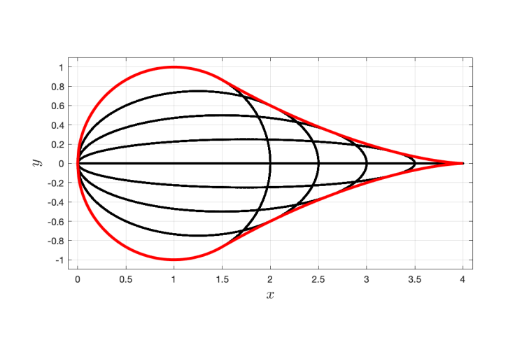
Figure 14: A sequence of five ellipses that contain the spectrum loci of the Laplacian matrices (24) as $c$ increases from $0$ to $1,$ including a unit circle $(c=0)$ and a segment $(c=1)$; the boundary $f_{1,2}(x)$ of a drop-shaped region, which is the union of all the ellipses (see Theorem 3), is shown in red

Theorem 3

Every eigenvalue of matrix (24) for any $c\in[0,~{}1]$ and ${\color[rgb]{0,0,0}N\in{\mathbb{N}}}$ lies in the drop-shaped region bounded by the functions

$${\color[rgb]{0,0,0}f_{1,2}(x)}\!=\!$$ (26)

$$\!\!\!\!\!\!\begin{cases}\pm\sqrt{1-(x-1)^{2}}&\!\!\mbox{if }x\!\in\!{\color[rgb]{0,0,0}[0,1.5]};\\ \pm\frac{1}{\sqrt{2}}(3\!-\!\sqrt{1+2x})\sqrt{\sqrt{1\!+\!2x}\!-\!x\!+\!1}&\!\!\mbox{if }x\!\in\!(1.5,4].\end{cases}$$

For ellipses (25), we have $x\in[0,2(1+c)]$ and $y\in[-(1-c),(1-c)],$ with the maximum and minimum at $x=1+c$ (cf. Fig. 14). Thus, for any two different ellipses of this family, each one extends beyond the other. Let us fix $c\in(0,1).$ Suppose that $(x_{cz},\pm y_{cz})$ with $x_{cz}\neq 0$ are the intersection points of the two ellipses corresponding to arc weights $c$ and $z\neq c.$ Then $x_{cz}$ increases in $z.$ Let $f_{z}(x)$ be the function representing the upper (non-negative) part of the ellipse corresponding to $z\in(0,1).$ We have

$$f_{z}(x)\!>\!f_{c}(x)\mbox{\;whenever\;}$$ (27)

$$((z\!<\!c)\,\&\,(0\!<\!x\!<\!x_{cz}))\mbox{\,or\,}((c\!<\!z)\,\&\,(x_{cz}\!<x\!\leq\!2+2c)).$$

Let

$$x_{c}=\mathop{\lim}\limits_{z^{\prime}\to c-0,\,z^{\prime\prime}\to c+0}x_{z^{\prime}z^{\prime\prime}}=\mathop{\lim}\limits_{z^{\prime}\to c-0}x_{z^{\prime}c}=\mathop{\lim}\limits_{z^{\prime\prime}\to c+0}x_{cz^{\prime\prime}}.$$

It follows from (27) that the only $x$ for which $f_{c}(x)=\mathop{\max}\limits_{z}f_{z}(x)$ is $x_{c}.$

Let us find $x_{c}$ as a function of $c$. To this end, we first find $x_{cz}$ as a function of $c$ and $z.$ Using (25) it is straightforward to verify that

$$x_{cz}=2\frac{\frac{(1-z)^{2}}{1+z}-\frac{(1-c)^{2}}{1+c}}{\left(\frac{1-z}{1+z}\right)^{2}-\left(\frac{1-c}{1+c}\right)^{2}}.$$ (28)

Now it can be shown that

$$x_{c}=\lim_{z\to c}x_{cz}=\frac{(1+c)(3+c)}{2},$$ (29)

and by (25) it holds that

$$f_{c}(x_{c})=\frac{1}{2}(1-c)\sqrt{(1-c)(3+c)}.$$ (30)

Substitution of the expression for $c$ from Eq. (29) into (30) yields the form of $f_{1,2}(x)$ given in Theorem 3.

In the following section, we show how the localization of the Laplacian spectra helps to analyze the stability of networks of high-order agents.

4 A Consensus Criterion

4.1 The Consensus Region

A system composed of agents (3) controlled by distributed protocol (4) can be equivalently represented as

$${\rm\bf a}(s)x={\rm\bf b}(s)(-\mathcal{L}_{N}x),$$ (31)

where $s:=\frac{d}{dt}$, $x=[x_{1},~{}x_{2},\ldots,x_{N}]^{\top}$, and $\mathcal{L}_{N}$ is the Laplacian matrix of the dependency digraph $\mathcal{G}_{N}$ containing a spanning converging tree.

The following condition simplifies the analysis of reaching consensus in system (31) by dividing the problem into two subproblems.

Definition 7 ( [35, 36, 34])

The consensus region (or $\Omega$-region) of the function $\phi(s)={\rm\bf a}(s)/{\rm\bf b}(s)$ in the Laplace variable $s$ is the set of points $\lambda$ in ${\mathbb{C}}$ for which the function $\phi(s)-\lambda$ has no zeros in the closed right half-plane:

$$\Omega=\{\lambda\in{\mathbb{C}}:\phi(s)-\lambda\neq 0~{}\text{\rm whenever }{\rm Re}(s)\geq 0\}.$$

The function $\phi(s)$ is sometimes referred to as the generalized frequency variable [49], [36].

Lemma 3 ( [35, 36, 34])

The network system with agents described by (3) reaches consensus under protocol (4) if and only if

$$\lambda_{i}\in\Omega,\quad i\in{\color[rgb]{0,0,0}\{2,\ldots,N\}},$$

where $\lambda_{i}$, $i\in{\color[rgb]{0,0,0}\{2,\ldots,N\}},$ are the nonzero eigenvalues of $-\mathcal{L}_{N}$.

The details of determining the consensus region may be found in [35]. In the case of $\phi(s)=s^{2}+\gamma s$, $\gamma>0,$ this region has the form of the interior of a parabola in the complex plane: $\phi(j\omega)=-\omega^{2}+j\gamma\omega$, $-\infty<\omega<\infty$, and if $\phi(s)=s$, then the $\Omega$-region is the open left half-plane of the complex plane.

4.2 Consensus in Systems on Ring Digraphs

In this subsection, we formulate and prove a consensus criterion for systems (31).

Theorem 4

A system (31), where $\mathcal{L}_{N}$ is the Laplacian matrix of a ring dependency digraph, reaches consensus in the sense of (8) for all numbers of agents if and only if the locus of the spectrum of $-\mathcal{L}_{N}$ lies entirely in the open consensus region $\Omega$ defined by $\phi(s)$ and shares only the point $(0,\,j0)$ with its boundary.

By Theorem 2, the Laplacian spectra of ring digraphs $\mathcal{G}_{m,n}$ obtained by round $m$-fold replication from a given simple ring $\mathcal{G}_{1,n}$ lie on a certain algebraic curve of order $2n$, irrespective of $m$. Taking this fact into account, it suffices to apply Lemma 3 to prove Theorem 4.

Remark 5

As mentioned above, Theorem 4 applies to systems whose ring topology always contains a spanning converging tree, which guarantees consensus in the case of first-order agents. Thus, this theorem gives additional conditions that ensure consensus at a higher order of agents.

4.3 Consensus in Networks of Second-Order Agents

Consensus problems in networks of second-order agents have been widely studied; see, e.g., [50, 51, 1, 52]. Here we consider the cases with absolute and relative velocity gain from the point of view of the consensus criterion of Theorem 4. Thus, the consensus conditions derived for the examples below are based on finding the intersection of the consensus region and the curve that contains the spectrum of system matrix  $-\mathcal{L}_{N}$. In some cases, we will use Vieta’s theorem.

Example 1

Consider the following system of $N$ interconnected second-order agents with absolute velocity gain $\gamma>0$ (see [48] for the details):

$$\ddot{x}+\gamma\dot{x}=-r\mathcal{L}_{N}x,$$ (32)

where $r>0$ is a scaling factor. This factor is introduced for the sake of generality and can be considered either as part of agent’s dynamics or as a parameter of the communication Laplacian matrix. In any case, matrix $-r\mathcal{L}_{N}$ now plays the role of $-\mathcal{L}_{N}$ in Theorem 4.

The consensus region of system (32) is bounded by the curve $\phi(j\omega)=-\omega^{2}+j\gamma\omega$, and the corresponding curve in ${\mathbb{R}}^{2}$ has the form $y^{2}=-\gamma^{2}x$. By Theorem 4, the system reaches consensus if and only if the spectrum of $-r\mathcal{L}_{N}$ belongs to the interior of the parabola $y^{2}=-\gamma^{2}x$ (except for the intersection at the origin) for all $N$.

Consider the communication topology represented by a Hamiltonian cycle (the classical cyclic pursuit illustrated by Fig. 1(a)) as the dependency digraph. The corresponding Laplacian matrix is given by (2); therefore, the eigenvalues of $-r\mathcal{L}_{N}$ are located on the circle of radius $r$ centered at $(-r,~{}j0)$. It is straightforward to check that this circle has no intersection with the above parabola except for the origin point whenever $r/\gamma^{2}\leq 1/2$. Note that this result for the “predecessor–follower” topology corresponds to the condition of asymptotic stability of the platoon solution in [29, Theorem 2], as $N$ tends to infinity.

If the dependency digraph has the form shown in Fig. 6, then the system reaches consensus in the sense of (8) if and only if the Cassini ovals (19) (Fig. 7) reflected about the vertical axis and $r$-scaled belong to the consensus region. This is satisfied whenever $r/\gamma^{2}\leq{7}/{6}$. In terms of the vehicular platoon control problem, this result means that the system becomes eventually unstable when the above inequality does not hold.

Figures 15 and 16 illustrate the cases where the condition of Theorem 4 is satisfied or violated.

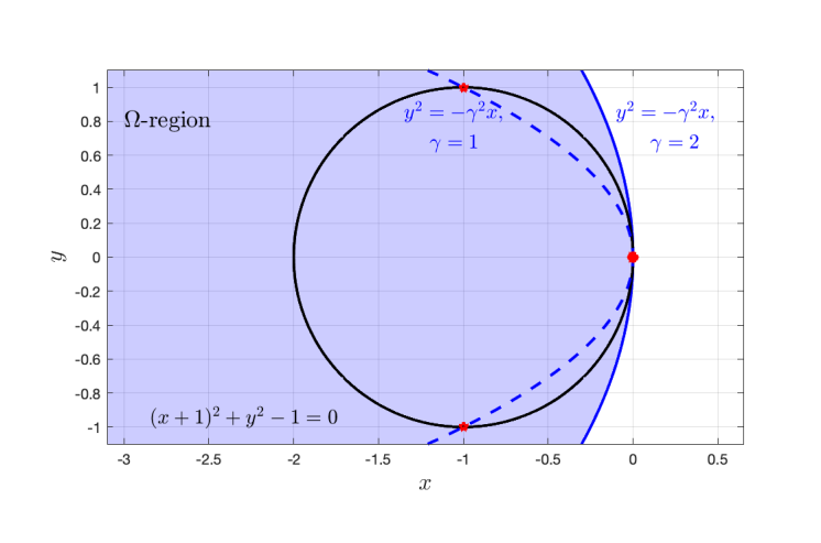
Figure 15: The $\Omega$-region bounded by $y^{2}=-\gamma^{2}x$ and the unit circle ($r=1$), where $\gamma\in\{1,~{}2\}$

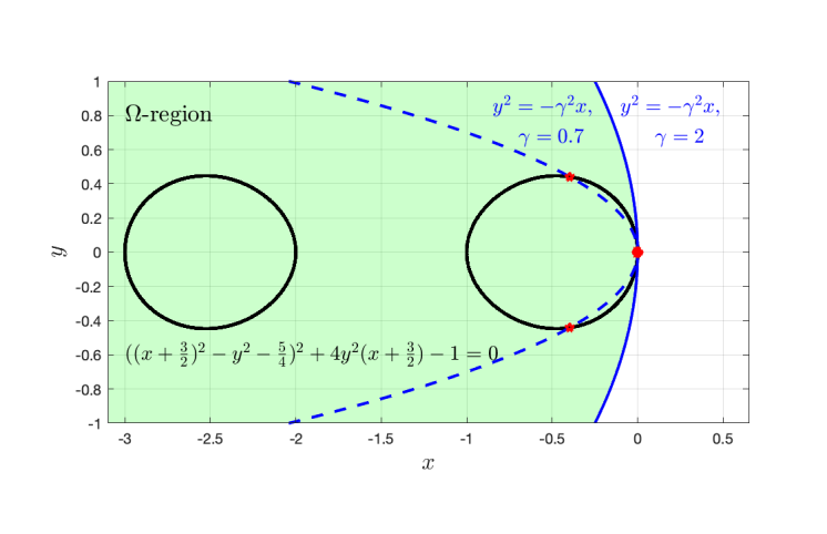
Figure 16: The $\Omega$-region bounded by $y^{2}=-\gamma^{2}x$ and the reflected Cassini ovals (19) ($r=1$), where $\gamma\in\{0.7,~{}2\}$

Example 2

Now consider the system

$$\ddot{x}=-r\mathcal{L}_{N}x-\gamma r\mathcal{L}_{N}\dot{x},\quad r>0$$ (33)

with relative velocity gain $\gamma>0$ and $r>0$.

Here the generalized frequency variable is $\phi(s)=s^{2}/(1+\gamma s)$. Since $\phi(j\omega)=-\omega^{2}/(1+\gamma^{2}\omega^{2})+j\gamma\omega^{3}/(1+\gamma^{2}\omega^{2})$, the boundary of the consensus region of system (33) on the plane ${\mathbb{R}}^{2}$ has algebraic expression $y^{2}=-\gamma^{2}x^{3}/(\gamma^{2}x+1)$.

Similarly to the previous example, consider two communication topologies and the two corresponding curves containing the spectrum of $-r\mathcal{L}_{N}$: (i) the circle of radius $r$ centered at $(-r,~{}j0)$ and (ii) the Cassini ovals (19) reflected about the vertical axis and $r$-scaled. In the first case, there always exists an intersection at $x=-2r/(1+2r\gamma^{2})$. In the second case, the corresponding cubic equation always has one negative real root $x_{0}$ regardless of the values of $r$ and $\gamma,$ as illustrated in Figs. 17 and 18.

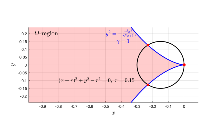
Figure 17: The $\Omega$-region bounded by $y^{2}=-\frac{\gamma^{2}x^{3}}{\gamma^{2}x+1}$ and the circle containing the spectrum of $-r\mathcal{L}_{N}$, where $\gamma=1$ and $r=0.15$

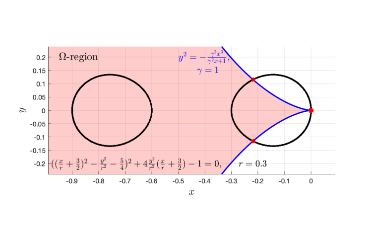
Figure 18: The $\Omega$-region bounded by $y^{2}=-\frac{\gamma^{2}x^{3}}{\gamma^{2}x+1}$ and the Cassini ovals containing the spectrum of $-r\mathcal{L}_{N}$, where $\gamma=1$ and $r=0.3$

Corollary 3

For system (33) with predefined relative velocity gain $\gamma$, no cyclic topology whose Laplacian spectrum belongs to the curve (13), (19), (21), (23), or (26) guarantees consensus for all $N\in{\mathbb{N}}$. For vehicle platoons control problems, this means that the system is eventually unstable.

Sketch of the proof:  Observe that both the curve $y^{2}=-\gamma^{2}x^{3}/(\gamma^{2}x+1)$ bounding the consensus domain of system (33) and the curve containing the Laplacian spectrum of $-r\mathcal{L}_{N}$ share the origin point $(0,~{}j0)$. Near this point, under a negative increment of $x$, the positive branch of any of the curves under consideration containing the Laplacian spectra of $-r\mathcal{L}_{N}$ grows faster than that of the curve $y^{2}=-\gamma^{2}x^{3}/(\gamma^{2}x+1),$ which can be straightforwardly confirmed by the analysis of derivatives. Therefore, starting from the origin, all the positive branches of the spectra curves lie above the positive branch of the boundary curve. Thus, they do not belong to the $\Omega$-region. Consequently, by Theorem 4, none of the topologies listed in Corollary 3 guarantees consensus for all $N\in{\mathbb{N}}.$

Remark 6

It follows from the analysis of the spectrum of $-r\mathcal{L}_{N}$ that system (33) with a certain value of the relative velocity gain $\gamma$ can reach consensus in the sense of (8), provided that the number of agents $N$ is sufficiently small. For example, for $\gamma=3.4$, the system with uni-directed topology reaches consensus if and only if $N\leq 6$. With a slightly increased factor $\gamma=4$, the system always reaches consensus if and only if $N\leq 7$, see Fig. 19.

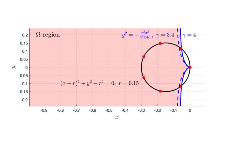
Figure 19: The $\Omega$-region bounded by $y^{2}=-\frac{\gamma^{2}x^{3}}{\gamma^{2}x+1}$, the circle that contains the spectra locus of $-r\mathcal{L}_{N}$ ($r=0.15$, $\gamma\in\{3.4,~{}4$}), and the eigenvalues of the matrix for $N=7$

Example 3

Let the system have the dynamics

$$\ddot{x}=-\frac{r}{\gamma}\mathcal{L}_{N}x+\left(r\mathcal{L}_{N}-\frac{1}{\gamma}I_{N}\right)\dot{x},\quad\gamma,r>0$$

and a more exotic generalized frequency variable $\phi(s)=(s+\gamma s^{2})/(1-\gamma s)$[36]. For $s=j\omega$ we have $\phi(j\omega)=-2\gamma^{2}\omega^{2}/(1+\gamma^{2}\omega^{2})+j\gamma(\omega-\gamma^{2}\omega^{3})/(1+\gamma^{2}\omega^{2})$, with the boundary of the consensus region $\Omega$ in ${\mathbb{R}}^{2}$ expressed as $y^{2}=-x(1+\gamma x)^{2}/(\gamma({\color[rgb]{0,0,0}2+\gamma x}))$.

Consider a uni-directed topology, whose Laplacian spectrum lies on a circle. It can be shown that the consensus condition of Theorem 4 is satisfied if and only if $r\gamma\leq 0.25$. The consensus region and two versions of the circle that contains the spectra locus of $-r\mathcal{L}_{N}$ are depicted in Fig. 20. Consensus is reached for $r=0.15,$ but this is not the case with $r=0.35$.

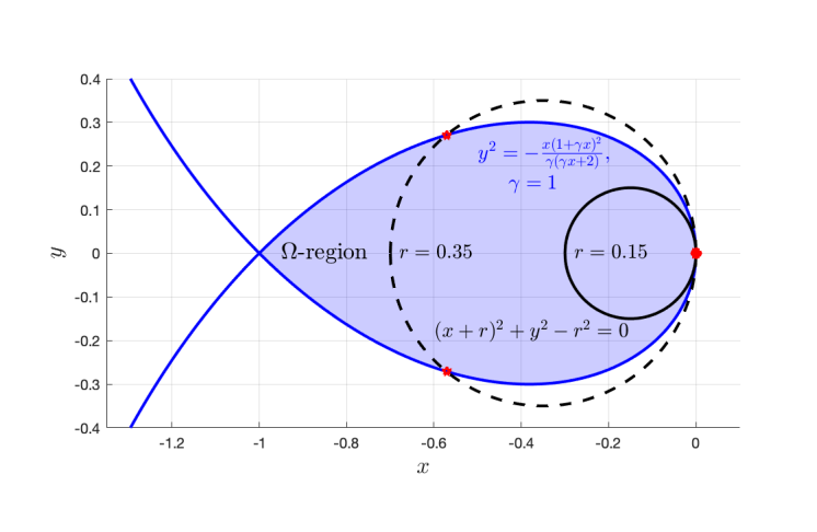
Figure 20: The $\Omega$-region bounded by $y^{2}=-x(1+\gamma x)^{2}/(\gamma(\gamma x+2))$ and the circles that contain the spectra loci of $-r\mathcal{L}_{N}$, where $r\in\{0.15,~{}0.35\}$ and $\gamma=1$

5 Conclusions

Cyclic pursuit is one of the most attractive and interesting problems of network communication. Its properties are studied using its Laplacian spectrum, which allows for exact localization on the unit circle. In this paper, we studied several versions of hierarchical cyclic pursuit, where each macro-vertex of the dependency digraph is a sequence of directed and bi-directional arcs.

The contribution of the paper is threefold. For the network dynamical systems on ring digraphs, we:

• proved that the corresponding Laplacian spectra lie on certain high-order algebraic curves regardless of the number of macro-vertices in the network;

• presented an algorithm for obtaining implicit equations of these curves;

• proposed a consensus condition in the frequency domain applicable to any number of agents in the network.

A characteristic feature of the algebraic curves obtained in this study is that they contain the spectrum loci of specific (Laplacian) matrices associated with network dynamical systems. Some of them, such as the Cassini ovals, have a simple geometric interpretation [53]; some others do not seem to have appeared in handbooks on special functions.

Possible extensions of this work include spectra localization of more general weighted networks that represent hierarchical pursuit. These problems are the subject of continuing research.

6 Acknowledgements

Research of P. Shcherbakov in Section IV was supported by the Russian Science Foundation (project No. 21-71-30005).

[]Sergei E. Parsegov received the M.S. degree in automation and control from Bauman Moscow State Technical University, Moscow, Russia, in 2008 and the Ph.D. (Candidate of Science) degree in physics and mathematics from the Institute of Control Sciences, Russian Academy of Sciences, in 2013. He is a Senior researcher in the Laboratory of Robust and Adaptive Systems, Russian Academy of Sciences. From 2018 he is with the Center for Energy Science and Technology of Skolkovo Institute of Science and Technology (Skoltech), Moscow. His research interests are dynamics and control of complex networks, opinion dynamics in social networks, distributed optimization and control in energy systems.

[]Pavel Yu. Chebotarev received the Ph.D. (Candidate of Science, 1990) and Doctor of Science (2008) degrees in physics and mathematics from the Institute of Control Sciences, Russian Academy of Sciences. He is the head of the Laboratory of Mathematical Methods for the Analysis of Multi-agent Systems. His research interests are in algebraic graph theory, clustering, decentralized control, voting theory, and social dynamics.

[]Pavel S. Shcherbakov was born in Moscow, Russia, in 1958. He received the M.S. degree in applied mathematics from the Department of Applied Mathematics, Moscow University of Transportation, in 1980, and the Candidate of Science degree (Russian equivalent of Ph.D.) and the Doctor of Science Degree both (in physics and mathematics) from the Institute of Control Science, Russian Academy of Sciences, Moscow, in 1991 and 2004, respectively. Since 1988, he has been with the Department of Robust and Adaptive Systems (Tsypkin Lab), Institute of Control Science, Moscow, where he is currently a Principal Researcher. His interests are in parametric robustness of control systems, probabilistic and randomized methods in control, linear matrix inequalities, and invariant ellipsoid methods in systems and control theory.

[]Federico Martín Ibáñez was born in Buenos Aires, Argentina, in 1982. He received the B.S. degree in electronic engineering from National Technological University (UTN), Buenos Aires, in 2008, and the Ph.D. degree in power electronics from the University of Navarra, San Sebastian, Spain, in 2012. From 2006 to 2009, he was with the Electronics Department, UTN. From 2009 to 2016, he was with the Power Electronics Group, Centro de Estudios e Investigaciones Tecnicas de Gipuzkoa. He is currently an Assistant Professor with the Center for Energy Science and Technology, Skoltech, Moscow, Russia. His research interests are in the areas of high-power dc–dc and dc–ac converters for applications related to energy storage, supercapacitors, electric vehicles, and smartgrids.

References

- [1] F. Bullo, Lectures on Network Systems (With contributions by J. Cortés, F. Dörfler, and S. Martínez), edition 1.6, 2022, http://motion.me.ucsb.edu/book-lns/
- [2] A. Rogozin, C. A. Uribe, A. V. Gasnikov, N. Malkovsky, and A. Nedić, “Optimal distributed convex optimization on slowly time-varying graphs,” IEEE Transactions on Control of Network Systems, vol. 7, no. 2, pp. 829–841, 2020.
- [3] P. Yu. Chebotarev and R. P. Agaev, “Coordination in Multiagent Systems and Laplacian Spectra of Digraphs,” Autom. Remote Control. vol. 70, no. 3, pp. 469–483, 2009.
- [4] C. Pozrikidis, An Introduction to Grids, Graphs, and Networks, Oxford: Oxford University Press, 2014.
- [5] H. Liu, M. Dolgushev, Y. Qi, and Z. Zhang, “Laplacian spectra of a class of small-world networks and their applications,” Scientific Reports, vol. 5, no. 9024, pp. 1–7, 2015.
- [6] A. Kammerdiner, A. Veremyev, and E. Pasiliao, “On Laplacian spectra of parametric families of closely connected networks with application to cooperative control,” Journal of Global Optimization, no. 67, pp. 187–205, 2017.
- [7] J. G. Darboux, “Sur un problème de géométrie élémentaire,” Bulletin des Sciences Mathématiques et Astronomiques, vol. 2, no. 1, pp. 298–304, 1878.
- [8] A. M. Bruckstein, N. Cohen, and A. Efrat, “Ants, crickets and frogs in cyclic pursuit,” Center Intell. Syst., Technion-Israel Inst. Technol, 1991.
- [9] A. M. Bruckstein, “Why the ant trails look so straight and nice,” The Mathematical Intelligencer, vol. 15, no. 2, pp. 59–62, 1993.
- [10] P. J. Nahin, Chases and Escapes: The Mathematics of Pursuit and Evasion, Princeton University Press, 2007.
- [11] B. R. Sharma, S. Ramakrishnan, and M. Kumar, “Cyclic pursuit in a multi-agent robotic system with double-integrator dynamics under linear interactions,” Robotica, vol. 31, no. 7, pp. 1037–1050, 2013.
- [12] Y. Elor and A. M. Bruckstein, “Uniform multi-agent deployment on a ring,” Theor. Comput. Sci., vol. 412, no. 8–10, pp. 783–795, 2011.
- [13] J. A. Marshall, M. E. Broucke, and B. A. Francis, “Formations of vehicles in cyclic pursuit,” IEEE Transactions on Automatic Control, vol. 49, no. 11, pp. 1963–1974, 2004.
- [14] S. L. Smith, M. E. Broucke, and B. A. Francis, “A hierarchical cyclic pursuit scheme for vehicle networks,” Automatica, vol. 41, no. 6, pp. 1045–1053, 2005.
- [15] W. Ding, G. Yan and Z. Lin, “Formations on two-layer pursuit systems,” IEEE International Conference on Robotics and Automation, 2009, pp. 3496-3501, 2009.
- [16] D. Mukherjee and D. Ghose,“Generalized hierarchical cyclic pursuit,” Automatica, vol. 71, pp. 318–323, 2016.
- [17] S. Parsegov, P. Shcherbakov, P. Chebotarev, V. Erofeeva, A. Rogozin, “Laplacian Spectra of Two-Layer Hierarchical Cyclic Pursuit Schemes,” IFAC-PapersOnLine, vol. 55, no. 13, pp. 246–251, 2022.
- [18] A. Sinha and D. Ghose, “Generalization of linear cyclic pursuit with application to rendezvous of multiple autonomous agents,” IEEE Transactions on Automatic Control, vol. 51, no. 11, pp. 1819–1824, 2006.
- [19] D. Mukherjee and S. R. Kumar, “Finite-Time Heterogeneous Cyclic Pursuit With Application to Cooperative Target Interception,” IEEE Transactions on Cybernetics, 2021, doi: 10.1109/TCYB.2021.3070955.
- [20] S. De, S. R. Sahoo, and P. Wahi, “Communication-delay-dependent rendezvous with possible negative controller gain in cyclic pursuit,” IEEE Transactions on Control of Network Systems, vol. 7, no. 3, pp. 1069–1079, 2020.
- [21] A. N. Elmachtoub and C. F. Van Loan, “From random polygon to ellipse. An eigenanalysis,” SIAM Rev., vol. 52, no. 1, pp. 151–170, 2010.
- [22] P. S. Shcherbakov, “Formation control: the Van Loan scheme and other algorithms,” Autom. Remote Control, vol. 72, no. 10, pp. 2210–2219, 2011.
- [23] J. L. Ramirez-Riberos, M. Pavone, E. Frazzoli, and D. W. Miller, “Distributed control of spacecraft formations via cyclic pursuit. Theory and experiments,” AIAA J. Guidance, Control, Dynamics, vol. 33, no. 5, pp. 1655–1669, 2010.
- [24] R. P. Agaev and P. Yu. Chebotarev, “A cyclic representation of discrete coordination procedures,” Autom. Remote Control, vol. 73, no. 1, pp. 161–166, 2012.
- [25] D. Mukherjee and D. Zelazo, “Robust consensus of higher order agents over cycle graphs,” in Proc. 58th Israel Annual Conference on Aerospace Sciences, pp. 1072–1083, 2018.
- [26] I. A. Wagner and A. M. Bruckstein, “Row straightening via local interactions,” Circuits Syst. Signal Process., vol. 16, no. 2, pp. 287–305, 1997.
- [27] Ya. I. Kvinto and S. E. Parsegov, “Equidistant arrangement of agents on line: analysis of the algorithm and its generalization,” Autom. Remote Control, vol. 73, no. 11, pp. 1784–1793, 2012.
- [28] A. V. Proskurnikov and S. E. Parsegov, “Problem of uniform deployment on a line segment for second-order agents,” Autom. Remote Control, vol. 77, no. 7, pp. 1248–1258, 2017.
- [29] J. A. Rogge and D. Aeyels, “Vehicle Platoons Through Ring Coupling,” in IEEE Transactions on Automatic Control, vol. 53, no. 6, pp. 1370–1377, 2008.
- [30] M. Pirani, S. Baldi, and K. H. Johansson, “Impact of Network Topology on the Resilience of Vehicle Platoons,” IEEE Transactions on Intelligent Transportation Systems, 2022.
- [31] S. Stüdli, M. M. Seron, and R. H. Middleton, “Vehicular platoons in cyclic interconnections,” Automatica, vol. 94, pp. 283–293, 2018.
- [32] I. Herman, D. Martinec, Z. Hurák, and M. Sebek, “Equalization of intervehicular distances in platoons on a circular track,” in Proc. of International Conference on Process Control, pp. 47–52, 2013.
- [33] P. Wieland, “From static to dynamic couplings in consensus and synchronization among identical and non-identical systems,” PhD thesis, https://elib.uni-stuttgart.de/handle/11682/4312, 2010.
- [34] Z. Li and Z. Duan, Cooperative Control of Multi-Agent Systems: A Consensus Region Approach, CRC Press, 2017.
- [35] B. T. Polyak and Y. Z. Tsypkin,“Stability and robust stability of uniform systems,” Autom. Remote Control, vol. 57, no. 11, pp. 1606–1617, 1996.
- [36] S. Hara, H. Tanaka, and T. Iwasaki, “Stability analysis of systems with generalized frequency variables,” IEEE Trans. Autom. Control, vol. 59, no. 2, pp. 313–326, 2014.
- [37] S. Stüdli, M. M. Seron, and R. H. Middleton, “From vehicular platoons to general networked systems: String stability and related concepts,” Annual Reviews in Control, vol. 44, pp. 157–172, 2017.
- [38] J. Monteil, G. Russo, and R. Shorten, “On string stability of nonlinear bidirectional asymmetric heterogeneous platoon systems,” Automatica, vol. 105, pp. 198–205, 2019.
- [39] E.C. Johnsen, “Essentially doubly stochastic matrices I. Elements of the theory over arbitrary fields,” Linear Algebra and Its Applications, vol. 4, no. 3, pp. 255–282, 1971.
- [40] E.R. Berlekamp, Algebraic Coding Theory, McGraw-Hill, NY, 1968.
- [41] E.L. Blanton, Jr., S.P. Hurd, and J.S. McCranie, “On the digraph defined by squaring mod , when has primitive roots,” Congressus Numerantium, vol. 82, pp. 167–177, 1991.
- [42] M.F. Barnsley, Fractals Everywhere, Academic Press, San Diego, 1988.
- [43] N.J.A. Sloan On-line Encyclopedia of Integer Sequences, https://oeis.org
- [44] R. P. Agaev and P. Yu. Chebotarev, “Which digraphs with ring structure are essentially cyclic?” Adv. Appl. Math. vol. 45, pp. 232–251, 2010.
- [45] V.V. Voevodin, Computational Principles of Linear Algebra (Vychislitel’nye osnovy lineinoi algebry), Nauka, Moscow, 1977 (in Russian). Translation: V. Voïévodine, Principes numériques d’algèbre linéaire, Mir, Moscow, 1980.
- [46] D.J. Uherka and A.M. Sergott, “On the continuous dependence of the roots of a polynomial on its coefficients,” American Math. Monthly, vol. 84, no. 5, pp. 368–370, 1977.
- [47] K. Hirose, “Continuity of the roots of a polynomial,” American Math. Monthly, vol. 127, no. 4, pp. 359–363, 2020.
- [48] S. Parsegov and P. Chebotarev, “Second-order agents on ring digraphs,” in Proc. ICSTCC, pp. 609–614, 2018.
- [49] S. Hara, T. Hayakawa, and H. Sugata, “Stability analysis of linear systems with generalized frequency variables and its applications to formation control,” in Proc. IEEE Conf. Decision Control, pp. 1459–1466, 2007.
- [50] W. Ren and Y. C. Cao, Distributed Coordination of Multi-Agent Networks, Springer, London, 2011.
- [51] D. Goldin, “Double integrator consensus systems with application to power systems,” in Proc. 4th IFAC Workshop NecSys-2013, pp. 206–211, 2013.
- [52] W. Ren, “On consensus algorithms for double-integrator dynamics,” IEEE Trans. Autom. Control, vol. 53, no. 6, pp. 1503–1509, 2008.
- [53] J. D. Lawrence, A Catalog of Special Plane Curves, Dover, New York, 1972.
[![[Uncaptioned image]](/html/2209.12178/assets/parsegov.png) ]Sergei E. Parsegov received the M.S. degree in automation and control from Bauman Moscow State Technical University, Moscow, Russia, in 2008 and the Ph.D. (Candidate of Science) degree in physics and mathematics from the Institute of Control Sciences, Russian Academy of Sciences, in 2013. He is a Senior researcher in the Laboratory of Robust and Adaptive Systems, Russian Academy of Sciences. From 2018 he is with the Center for Energy Science and Technology of Skolkovo Institute of Science and Technology (Skoltech), Moscow. His research interests are dynamics and control of complex networks, opinion dynamics in social networks, distributed optimization and control in energy systems.