Replica approach to the generalized Rosenzweig-Porter model

Davide Venturelli^1$\star$, Leticia F. Cugliandolo^2,3, Grégory Schehr² and Marco Tarzia^3,4

Abstract

The generalized Rosenzweig-Porter model with real (GOE) off-diagonal entries arguably constitutes the simplest random matrix ensemble displaying a phase with fractal eigenstates, which we characterize here by using replica methods. We first derive analytical expressions for the average spectral density in the limit in which the size $N$ of the matrix is large but finite. We then focus on the number of eigenvalues in a finite interval and compute its cumulant generating function as well as the level compressibility, i.e., the ratio of the first two cumulants: these are useful tools to describe the local level statistics. In particular, the level compressibility is shown to be described by a universal scaling function, which we compute explicitly, when the system is probed over scales of the order of the Thouless energy. Interestingly, the same scaling function is found to describe the level compressibility of the complex (GUE) Rosenzweig-Porter model in this regime. We confirm our results with numerical tests.

 

Contents

1. 1 Introduction
   1. 1.1 The generalized Rosenzweig-Porter model
   2. 1.2 Outline of this work and summary of the main results
2. 2 Average spectral density
   1. 2.1 Saddle-point equations and rotationally-invariant Ansatz
   2. 2.2 General result
      1. 2.2.1 Limiting cases
   3. 2.3 Resolvent formulation and connection with the Zee formula
   4. 2.4 Exactly solvable cases
      1. 2.4.1 Cauchy distributed $a_{i}$
      2. 2.4.2 Wigner distributed $a_{i}$
   5. 2.5 Approximate solutions
3. 3 Number of eigenvalues in an interval and level compressibility
   1. 3.1 Replica action and saddle-point equations
   2. 3.2 Rotationally-invariant Ansatz
   3. 3.3 General result in the case of a symmetric interval
      1. 3.3.1 Limit of a pure diagonal matrix with random i.i.d. entries
      2. 3.3.2 Limit of a pure GOE matrix
   4. 3.4 Exactly solvable cases
      1. 3.4.1 Cauchy distributed $a_{i}$
      2. 3.4.2 Wigner distributed $a_{i}$
   5. 3.5 Scaling limit and Thouless energy
   6. 3.6 Behavior for small $E$
4. 4 Conclusions
5. A Number of i.i.d. variables in an interval
6. B Details of the replica calculation of the spectral density
7. C Connection with the Zee formula
8. D Details of the replica calculation of the level compressibility
   1. D.1 Functional representation
   2. D.2 Gaussian fluctuations around the saddle-point
9. E Level compressibility in the pure GOE case
   1. E.1 Action and fluctuations around the saddle-point
   2. E.2 Case of a symmetric interval
   3. E.3 Derivation of the scaling function $\chi_{\rm GOE}(y)$
10. F Scaling function for the Hermitian GRP model

 

1 Introduction

Quantum non-interacting particles in a disordered potential undergo the Anderson localization transition as the disorder strength is increased [1]. In one and two dimensions an infinitesimal amount of disorder is sufficient to localize all eigenstates of the Hamiltonian, while in dimension larger than two a critical value of the disorder strength separates a metallic phase, where the eigenstates are similar to plane waves and spread over the whole volume uniformly, from an insulating phase, where the eigenstates are instead exponentially localized around specific points in space, and thereby occupy a finite $\mathcal{O}(1)$ portion of the total volume. It is well established that exactly at the Anderson localization critical point the wave-functions are multifractal [2, 3]. This means that they are neither fully delocalized (as in the metallic regime), nor fully localized (as in the insulating phase), since their support set grows with the system size but remains a vanishing fraction of the total volume. The multi-fractal character of the wave functions is due to the fact that the $q$th moments of their amplitudes decay with the size $N$ as $\langle\sum_{i=1}^{N}|\psi_{i}|^{2q}\rangle\propto N^{-(q-1)D_{q}}$, with different $q$-dependent exponents $0\leq D_{q}\leq 1$.

In the last decade, the Hilbert space localization properties of quantum disordered many-body systems have attracted much interest. In this context, the emergence of multifractal states has been discussed as a key and robust feature of their phase diagram, and has been invoked to explain some of their unconventional properties beyond the single-particle limit. In the many-body setting, multifractal eigenstates that do not cover the whole accessible Hilbert space may lead to the violation of the eigenstate thermalization hypothesis (ETH) [4, 5]. Therefore, they are often called partially delocalized but non-ergodic, in contrast to the ergodic fully delocalized eigenstates, which are supposed to satisfy ETH.

In the context of Many Body Localization (MBL), recent studies indicate that the many-body eigenstates are in fact multifractal in the whole insulating phase [6, 7, 8, 9, 10, 11, 12, 13]. Furthermore, the seminal work by Basko, Aleiner and Altshuler [14] predicted the existence of a novel unconventional “bad metal” regime in between the fully ergodic metallic phase at low disorder and the insulating one at strong disorder. Following the pioneering ideas of [15], the unusual properties of the bad metal regime have also been put in relation with the possible multifractal nature of the many-body eigenstates. Recent investigations of the out-of-equilibrium phase diagram of the quantum random energy model [16, 17, 18, 19, 20] and Josephson junction arrays [21, 22] seem to support this scenario. The existence of partially extended but non-ergodic wave-functions is also believed to have relevant practical and conceptual implications in the efficient population transfer in the context of quantum computing [19, 20, 23]. Moreover, recent studies of the Sachdev-Ye-Kitaev model in high-energy physics and quantum gravity have reported evidence for the emergence of a non-ergodic, but partially extended phase when the model is perturbed by a single-body term [24, 25].

Matrix models have been an invaluable tool to describe and help understanding complex physical systems, in particular those with quenched randomness. The physical mechanism at the origin of the above-mentioned multiftactal eigenstates is one such problem, and specific matrix models have recently been used as proxies which capture the peculiar spectral properties associated with them. In this respect, the Rosenzweig-Porter (RP) random matrix ensemble [26], originally introduced to reproduce the spectral properties of complex atomic spectra, provides an archetypal illustration of a system in which a partially extended phase featuring fractal eigenstates (along with other unconventional spectral properties that will be extensively discussed below) appears in an intermediate region of the phase diagram between a fully delocalized phase and a fully Anderson localized phase (see Fig. 1). For this reason the RP model has been the focus of a strong resurgence of attention over the last few years [27, 28, 29, 30, 31, 32, 33, 34, 35]. Although one cannot expect that simple random matrix models could capture all the properties of interacting quantum systems, they provide natural and powerful tools to understand the deep physical mechanisms behind some of their features, which are often elusive to analytical treatments in more realistic settings.

The Hamiltonian of the RP model $\mathcal{H}=A+c(N)B$ can be written as the sum of an $N\times N$ diagonal matrix $A$, whose entries $a_{i}$’s are independent and identically distributed (i.i.d.) random variables drawn from a Gaussian distribution $p_{a}(a_{i})$, and another $N\times N$ random matrix $B$ belonging to the Gaussian orthogonal (or unitary) ensemble (GOE or GUE, respectively). If the variances of the matrix elements $b_{ij}$ are chosen of $\order{1}$, then the width of the spectrum of $B$ is of $\order{\sqrt{N}}$: thus the matrix $A$ (whose spectral width is of $\order{1}$) can produce significant deviations from the GOE/GUE behavior only if $c(N)$ decays sufficiently fast for large $N$. The properties of this model have been extensively studied by using different techniques, such as a mapping to the Dyson Brownian motion [36], supersymmetry [37, 38], resolvent methods [39, 40], and first order perturbation theory [41].

Due to the strong surge of attention towards multifractal states in quantum many-body disordered systems, a generalized version of the RP model in which the distribution $p_{a}(a_{i})$ is not necessarily Gaussian has then been introduced in Ref. [27], and thoroughly investigated by using the techniques recalled above [28, 29, 30, 31, 32, 33, 34, 35] – we will refer to this as the GRP model. In addition, new connections and applications have been pointed out in disordered elastic systems [42], many-body localization [16, 17, 18, 9], quantum gravity [24, 25], quantum information [19, 23, 20], models of theoretical ecology [43], and noise reduction in big data matrices [44].

In this work we revisit the generalized RP model by analyzing some properties of the energy levels and their correlations which have not been investigated in the literature yet. In particular, we perform a thorough study of the finite-$N$ corrections to the average spectral density and compute the level compressibility in the intermediate phase, thereby providing a deeper understanding of the properties of the intermediate regime. Our analysis uses the replica method largely exploited in the analysis of spin glass models [45], but not only – for example, this tool has been recently applied to study the properties of the ground states in a deformed GOE ensemble [46]. Our replica study is developed for the case in which the entries of $\mathcal{H}$ are real numbers, so that $\mathcal{H}$ belongs to a deformed GOE ensemble (where the deformation is introduced by the addition of the diagonal random matrix $A$). However, and quite surprisingly, we show that the exact same behavior of the level compressibility applies to the crossover regime of the Hermitian GRP model [27] (in which the off-diagonal entries are complex).

In the rest of this introductory section we will present the RP model and some of its salient properties (Section 1.1), and we will outline our study and main results (Section 1.2).

Figure 1: Sketch of the different phases of the RP model, depending on the value of the parameter $\gamma$ in Eq. 1. Considering the average spectral density $\rho(\lambda)$, a transition is first observed at $\gamma=1$ which separates a fully delocalized phase where $\rho(\lambda)=\rho_{\text{GOE}}(\lambda)$ from a partially delocalized phase where $\rho(\lambda)=p_{a}(\lambda)$ in the thermodynamic limit (see the main text). Focusing instead on the local level statistics, another transition is found at $\gamma=2$ from the partially delocalized phase characterized by the Wigner-Dyson statistics, to an Anderson-localized phase characterized by the Poisson statistics. The shaded region $1<\gamma<2$ indicates the intermediate phase studied in this work.

1.1 The generalized Rosenzweig-Porter model

We consider the Hamiltonian represented by the $N\times N$ matrix

$$\mathcal{H}=A+\frac{\nu}{N^{\gamma/2}}B\,,$$ (1)

where the matrix $B$ belongs to the GOE ensemble: its elements are Gaussian random variables with zero mean and unit variance (i.e., $\langle b_{ii}^{2}\rangle=1$ and $\langle b_{ij}^{2}\rangle=1/2$ for $i\neq j$). With this choice, the spectrum of $B$ in the limit $N\to\infty$ converges to a Wigner semicircle supported within $\lambda\in[-\sqrt{2N},\sqrt{2N}]$, where we denote hereafter with $\lambda$ the eigenvalues of $\mathcal{H}$. The parameter $\nu$ is of $\order{1}$ and does not scale with $N$. The deformation matrix $A$ is instead diagonal, with independent entries $a_{i}$’s identically distributed according to a generic distribution $p_{a}(a)$, hence the name Generalized Rosenzweig-Porter model (GRP).

Following the analogy with disordered quantum many-body systems, each matrix index can be thought of as a site of the reference Hilbert space, which is connected to every other site with the transition rates distributed according to the Gaussian law. Different phenomenologies are expected depending on the value of the parameter $\gamma$, which renders one of the two matrices $A$ or $B$ subleading with respect to the other in the limit of large $N$. As summarized in Fig. 1, the model features three distinct phases (and two transition points between them): a fully delocalized phase for $\gamma<1$, a fully Anderson localized phase for $\gamma>2$, and an intermediate fractal phase for $1<\gamma<2$.

The transition from fully extended to fractal eigenstates at $\gamma=1$ manifests itself as a transition for the average spectral density $\rho(\lambda)$, which reproduces the Wigner semicircle law for $\gamma<1$ in the $N\to\infty$ limit, while it reduces to $\rho(\lambda)=p_{a}(\lambda)$ if $\gamma>1$ and the same $N\to\infty$ limit is taken. At $\gamma=1$, $\rho(\lambda)$ interpolates between $p_{a}(\lambda)$ and the Wigner semicircle as the value of the parameter $\nu$ is increased. This transition becomes sharp (i.e., it occurs at a particular value of $\nu=\nu_{c}$) provided that $p_{a}(a)$ has a compact support and vanishes sufficiently fast at its upper edge [47, 42].

The value $\gamma=2$ corresponds instead to a genuine Anderson localization transition. Indeed, the region $\gamma<1$ is characterized by the Wigner-Dyson statistics, meaning that the eigenvectors of $\mathcal{H}$ are uniformly delocalized on $N$ sites in the large $N$ limit, and the average level spacing follows the Wigner surmise [48], signaling level repulsion. Conversely, in the region $\gamma>2$ the eigenvectors are completely localized over $\mathcal{O}(1)$ sites and the mean level spacing exhibits Poisson statistics.

The intermediate region with $1<\gamma<2$ is particularly interesting, because the average spectral density tends to $p_{a}(\lambda)$, but the local level statistics remains of the Wigner-Dyson type. Here the eigenvectors are known to be delocalized over a large number of sites $N^{D_{\gamma}}$, which represent, however, a vanishing fraction of the total number of sites $N$ in the thermodynamic limit, their fractal dimension being $D_{\gamma}=2-\gamma<1$ [27].

The simplest and most intuitive way to understand the spectral properties in the intermediate region is provided by the Fermi golden rule. In the limit in which the off-diagonal matrix $B$ is absent and all the eigenvectors are trivially localized on a single site, one has $|\psi_{i}\rangle=|i\rangle$, with corresponding eigenenergies $\lambda_{i}=a_{i}$. When the GOE perturbation $\nu N^{-\gamma/2}B$ is turned on, the transition probability per unit time from a state $i$ to another state $j$ can be evaluated perturbatively as

$$\Gamma_{i\to j}=\frac{2\pi\rho}{\hbar}\frac{4\eta}{N}|b_{ij}|^{2}\,,$$

where $\rho=\rho(\lambda)$ and, for future convenience, we have introduced the combination

$$\eta\equiv N^{1-\gamma}\nu^{2}/4\,.$$ (2)

Hence, the average escape rate per unit time for a “particle” created in site $i$ at time $t=0$ reads

$$\Gamma=\sum_{j\neq i}\langle\Gamma_{i\to j}\rangle=\frac{2\pi\rho}{\hbar}4\eta\,.$$ (3)

The quantity $\hbar\Gamma$ can thus be interpreted as the bandwidth $\Delta E$ that can be reached in a time of $\mathcal{O}(1)$ from a given site $i$:

$$\Delta E\sim\hbar\Gamma\;.$$

This implies that the eigenvectors within this energy window are hybridized by the GOE perturbation. For $1<\gamma<2$ such energy band decays with the system size as $\Delta E\propto N^{1-\gamma}$ but is much larger than the mean level spacing

$$\delta_{N}\simeq[N\rho]^{-1}\,,$$ (4)

entailing that the system is not Anderson localized; still, $\Delta E$ remains much smaller than the total bandwidth, which is of $\mathcal{O}(1)$. This signifies that the particle can only explore a sub-extensive portion of the total volume. The Anderson localization transition thus occurs when $\Delta E$ becomes smaller than the mean level spacing, i.e., for $\gamma\geq 2$: this implies that the average escape time from site $i$ (i.e., $\Delta t\equiv\hbar/\Delta E$) grows at least linearly with $N$, and thus the eigenfunctions remain localized on $\mathcal{O}(1)$ sites. Conversely, the transition to the fully delocalized phase takes place when $\Delta E$ becomes of the order of the total bandwidth, i.e., for $\gamma\leq 1$: this implies that, starting from site $i$, the wave-packet can reach any other site in a time of $\mathcal{O}(1)$.

In the intermediate phase, $1<\gamma<2$, the support set of the eigenvectors (i.e., the number of sites which are hybridized by the perturbation) is simply given by the spreading of the energy interval divided by the average gap between adjacent energy levels, and thus scales as $\Delta E/\delta_{N}\sim N^{D_{\gamma}}$, with $D_{\gamma}=2-\gamma$. The partially extended but fractal eigenstates are therefore linear combinations of a bunch of $N^{D_{\gamma}}$ localized states associated to nearby energy levels, i.e.,

$$|\psi_{i}\rangle\approx\!\!\sum_{\begin{subarray}{c}i^{\prime}\;s.t.\\ |a_{i}-a_{i}^{\prime}|\leq\Delta E\end{subarray}}\!\!c_{i^{\prime}}\,|i^{\prime}\rangle\,,$$

with coefficients $c_{i^{\prime}}$ of order $N^{-D_{\gamma}/2}$ to ensure normalization. These eigenstates give rise to the so-called mini-bands in the local spectrum [27]. The width of the mini-bands sets the energy scale

$$E_{T}\sim\Delta E\sim N^{D_{\gamma}-1}=N^{1-\gamma}\,,$$ (5)

often called the Thouless energy [49, 50], within which GOE-like spectral correlations (and in particular level repulsion) have been established. All the moments of the wave-functions’ coefficients (the so-called generalized inverse participation ratios, IPR) behave as

$$I_{q}=\sum_{i}|\langle i|\psi\rangle|^{2q}\propto N^{D_{\gamma}(1-q)}\qquad\quad\implies\qquad\quad D_{q}=D_{\gamma}\;.$$ (6)

This implies that all the fractal dimensions $D_{q}$ are degenerate and equal to $D_{\gamma}$ for all positive integer $q$, i.e., that the intermediate phase of the GRP model is fractal but not multifractal.

As discussed above, the emergence of such fractal phase is particularly relevant in many physical contexts. Its existence was first suggested in Kravtsov_2015,Refs. Ref. [27] and then rigorously proven in vonSoosten_2019,Refs. Ref. [28]. In recent years several generalizations of the RP model have been put forward and analysed [51, 52, 53, 54, 55, 56], and many other random matrix ensembles have been shown to have an intermediate partially delocalized phase with similar spectral properties [57, 58, 59, 60, 61, 62, 63, 64, 65, 66, 67, 68, 69, 70, 71, 72]. Yet, the GRP setting is still a very useful playground to analyze the properties of fractal states in a controlled framework.

1.2 Outline of this work and summary of the main results

As explained above, the GRP model has been intensively investigated over the past few years with a great variety of analytical and numerical techniques. In this paper we tackle this model by applying yet another approach, namely the replica formalism [45], which allows us to obtain new results on the average spectral density, and the statistics of the number of energy levels within a finite interval.

In Section 2 we start by analyzing the average density of states $\rho(\lambda)$. When the size $N$ of the matrix is large, we find the leading order estimate

$$\rho(\lambda)=-\frac{1}{\pi\eta}\lim_{\varepsilon\to 0^{+}}\real C(\lambda_{\varepsilon})+\order{1/N}\,,$$ (7)

where $\lambda_{\varepsilon}=\lambda-i\varepsilon$, the parameter $\eta$ depends on $N$ and was introduced in Eq. 2, and the function $C(\lambda)$ is implicitly defined by the self-consistency equation

$$C(\lambda)=i\eta\,\mathcal{G}_{a}\left[\lambda+2iC(\lambda)\right]\,.$$ (8)

Here $\mathcal{G}_{a}$ is the resolvent associated to the distribution $p_{a}(a)$ of the entries of $A$ (c.f. Eq. 43). In general, it is quite difficult to solve explicitly Eq. 8 for $C(\lambda)$ for any arbitrary distribution $p_{a}(a)$. However, we show in Section 2.4 that it can be solved explicitly for two special cases: (i) when $p_{a}(a)$ is a Wigner semicircle – which is expected, since it is stable under free-convolution [73] – and (ii) when it is a Cauchy distribution, which is more surprising.

As we show in Section 2.3, by taking the limit $N\to\infty$ with $\eta$ kept finite, Eqs. 7 and 8 reduce to the free addition formula [73], sometimes called the “Zee formula” in the physics literature [74]. However, as we show in Section 2.5, these equations contain more information and, in the case where $\eta=\eta(N)\ll 1$ defined in Eq. 2 with $1<\gamma<2$, they allow us to obtain the leading $1/N$ corrections to the limiting density $\rho(\lambda)=p_{a}(\lambda)$ in a controlled way, even when the resolvent $\mathcal{G}_{a}(z)$ does not admit a closed-form analytic expression. These corrections turn out to be quite difficult to compute using the standard free addition formula, which in principle holds only in the limit $N\to\infty$.

Next, in Section 3 we analyze the behavior of the level compressibility $\chi(E)$, which is a simple indicator of the degree of level repulsion and is defined as follows[78]. We first introduce the empirical density of the (real) eigenvalues $\lambda_{i}$ of $\cal{H}$, defined as

$$\rho_{N}(\lambda)=\frac{1}{N}\sum_{i=1}^{N}\delta(\lambda-\lambda_{i})\,.$$ (9)

Note that $\rho_{N}(\lambda)$ is normalised to unity. Let

$$I_{N}[\alpha,\beta]\equiv N\int_{\alpha}^{\beta}\differential{\lambda}\rho_{N}(\lambda)$$ (10)

denote the number of eigenvalues lying in the interval $[\alpha,\beta]\subseteq\mathbb{R}$, which is a random variable. Then

$$\chi(E)\equiv\frac{\kappa_{2}(E)}{\kappa_{1}(E)}=\frac{\expectationvalue{I_{N}^{2}[-E,E]}-\expectationvalue{I_{N}[-E,E]}^{2}}{\expectationvalue{I_{N}[-E,E]}}=\frac{\expectationvalue{I_{N}^{2}[-E,E]}_{c}}{\expectationvalue{I_{N}[-E,E]}}\,,$$ (11)

where $\kappa_{1}$ and $\kappa_{2}$ are the first two cumulants of $I_{N}$. For Poisson statistics, one has $\kappa_{2}(E)\simeq\kappa_{1}(E)$ for small $E$, and then $\chi(E)\simeq 1$ (see Appendix A). On the contrary, for a rigid spectrum like that of the GOE matrix $B$ in Eq. 1, the mean number of eigenvalues behaves as $\expectationvalue{I_{N}[-E,E]}\propto\tilde{E}$, with $\tilde{E}\equiv N\rho_{N}(0)\,E$ and where $[N\rho_{N}(0)]^{-1}$ is the mean level spacing close to $E=0$, while $\expectationvalue{I_{N}^{2}[-E,E]}_{c}\propto\ln\tilde{E}$ for large $\tilde{E}$. Hence in the GOE case one finds $\chi(E)\to 0$ for $\tilde{E}\to\infty$, i.e., for $E\gg[N\rho_{N}(0)]^{-1}$ (but still much smaller than $E\sim\order{1}$).

In Section 3.3 we provide the cumulant generating function of the variable $I_{N}[\alpha,\beta]$ at leading order for large $N$. For a symmetric interval $[-E,E]$ and a symmetric distribution $p_{a}(a)$, the result reads

$$\mathcal{F}_{[-E,E]}(s)\equiv\frac{1}{N}\ln\expectationvalue{e^{-sI_{N}[-E,E]}}=-ms+\ln\expectationvalue{e^{-sf(a)}}_{a}+\order{\eta/N}\,,$$ (12)

where

$$m=-\frac{2\eta}{\pi}\imaginary\left[\mathcal{G}_{a}\left(-i\Delta^{-1}\right)\right]^{2}\,,\;\;\;\;\;f(a)\equiv\frac{1}{\pi}\arctan\left(\frac{\sin 2\theta}{a^{2}r^{2}+\cos 2\theta}\right)\in[0,1]\,,$$ (13)

and $\Delta(E)=r(E)e^{i\theta(E)}$ has to be determined by solving the self-consistency equation

$$\Delta^{-1}=\varepsilon-iE-2i\eta\mathcal{G}_{a}\left(-i\Delta^{-1}\right)\,,$$ (14)

before sending $\varepsilon\to 0$. Again, we show that a closed-form solution can be found in some particular cases. Our results are supported by the comparison with the numerical diagonalization of large random matrices.

The ratio of the first two cumulants of $I_{N}[-E,E]$ gives the level compressibility $\chi(E)$ introduced in Eq. 11. In agreement with the picture presented above for the region $1<\gamma<2$, and having identified $E_{T}\propto\eta\propto N^{1-\gamma}$ as the Thouless energy of the system, we explicitly verify in Section 3.5 that $\chi(E)\sim 0$ for $E\ll E_{T}$ – but still much larger than the mean level spacing $\delta_{N}\propto N^{-1}$ – corresponding to level repulsion, while $\chi(E)$ follows the Poisson statistics for $E\gg E_{T}$. However, in the scaling limit $E=2\pi p_{a}(0)\eta\cdot y$ with $N^{-1}\ll\eta\ll 1$, we show that $\chi(E)$ takes the universal form

$$\chi(E)\simeq\chi_{T}\left(y=\frac{E}{2\pi p_{a}(0)\eta}\right)\,,\quad\quad\chi_{T}(y)=\frac{1}{\pi y}\left[2y\arctan(y)-\ln(1+y^{2})\right]\,,$$ (15)

where the scaling function $\chi_{T}(y)$ is independent of the specific choice of $p_{a}(a)$. This function is plotted in Fig. 6: it behaves as $\chi_{T}(y)\simeq y/\pi$ for small $y$, while it tends to $1$ for large $y$. Note that the crossover energy scale $2\pi p_{a}(0)\eta$ coincides (apart from a factor of $4$) with the width of the mini-bands identified in Eq. (3) using the Fermi golden rule, which allows us to put the intuitive arguments given above on the structure of spectral correlations on a much firmer basis.

Interestingly, using results from Refs. [27] and [40], we show that the same scaling function $\chi_{T}$ also describes the crossover for Hermitian $B$ matrices – while the level compressibilities for the real and the Hermitian GRP ensembles differ outside of this energy regime. We do so by relating the level compressibility to the 2-level spectral correlation function of the Hermitian GRP model, previously derived in [40, 27] by means of the Harish-Chandra-Itzykson-Zuber integral (which notably does not admit a counterpart for matrices with real entries).

In Section 3.6 we finally inspect, using extensive numerical diagonalization of large random real matrices, the low-energy region where $E$ is chosen on the scale of the Thouless energy. The scaling form of $\chi(E)$ presented in Eq. 15 is thus shown to represent a universal crossover between the classical GOE result $\chi(E\sim N^{-1})\simeq\chi_{\text{GOE}}(E)$ for energies of the order of the mean level spacing (and much smaller than the Thouless energy, see Eq. E.25), and the model-dependent prediction of Eqs. 11 and 12, valid for energies of the order of the total spectral band-width, i.e., $E\sim\order{1}$.

2 Average spectral density

Let us begin by considering the density of states of the matrix $\mathcal{H}$ in Eq. 9. Its mean value can be obtained by means of the Edwards-Jones (E-J) formula [79, 48], which we briefly recall here. One starts from the Plemelj-Sokhotski relation: if $f(x)$ is a complex-valued function which is continuous on the real axis, and given $\alpha<0<\beta$, then

$$\lim_{\varepsilon\to 0^{+}}\int_{\alpha}^{\beta}\differential{x}\frac{f(x)}{x\pm i\varepsilon}=\mp i\pi f(0)+\principalvalue{\int_{\alpha}^{\beta}\differential{x}\,\frac{f(x)}{x}}\,,$$ (16)

where $\principalvalue$ indicates the Cauchy principal value of the integral. From Eq. 9 we then have

$$\expectationvalue{\rho_{N}(\lambda)}=\frac{1}{\pi N}\lim_{\varepsilon\to 0^{+}}\imaginary\expectationvalue{\sum_{i=1}^{N}\frac{1}{\lambda-\lambda_{i}-i\varepsilon}}=\frac{1}{\pi N}\lim_{\varepsilon\to 0^{+}}\imaginary\partialderivative{\lambda}\expectationvalue{\sum_{i=1}^{N}\ln(\lambda_{i}-\lambda+i\varepsilon)}\,,$$ (17)

where the average is taken over the distribution of the entries of $\mathcal{H}$. In the last step we indicated by $\ln(z)$ the principal branch of the complex logarithm. Using the properties of Gaussian integrals, we finally obtain the E-J formula [79]

$$\rho(\lambda) \equiv\expectationvalue{\rho_{N}(\lambda)}=-\frac{2}{\pi N}\lim_{\varepsilon\to 0^{+}}\imaginary\derivative{\lambda}\expectationvalue{\ln\mathcal{Z}(\lambda_{\varepsilon})}\,,$$ (18)

$$\mathcal{Z}(\lambda) \equiv\det(\mathcal{H}-\lambda\mathbb{1})^{-1/2}=(2\pi i)^{-N/2}\int_{\mathbb{R}^{N}}\differential{\mathbf{r}}e^{-\frac{i}{2}\mathbf{r}^{T}(\lambda\mathbb{1}-\mathcal{H})\mathbf{r}}\,,$$ (19)

where $\lambda_{\varepsilon}\equiv\lambda-i\varepsilon$ with $\varepsilon>0$. Note that the negative imaginary part of $\lambda_{\varepsilon}$ ensures the convergence of the integral in Eq. 19. The expectation value of the logarithm can then be handled by using the replica trick [45]

$$\expectationvalue{\ln\mathcal{Z}(\lambda)}=\lim_{n\to 0}\frac{1}{n}\ln\expectationvalue{\mathcal{Z}^{n}(\lambda)}\,,$$ (20)

which allows us to trade the quenched average on the left-hand-side for the annealed average on the right-hand-side. The latter can be evaluated by standard methods (see Appendix B) to give

$$\expectationvalue{\mathcal{Z}^{n}(\lambda)}\propto\int\mathcal{D}\mu\,\mathcal{D}\hat{\mu}\,e^{N\mathcal{S}_{n}[\mu,\hat{\mu};\lambda]}\,,$$ (21)

where the proportionality holds up to an irrelevant numerical constant, and where we introduced the action

$$\mathcal{S}_{n}[\mu,\hat{\mu};\lambda]\equiv -i\int\differential{\vec{y}}\mu(\vec{y})\hat{\mu}(\vec{y})-\frac{\eta}{2}\int\differential{\vec{y}}\differential{\vec{w}}\mu(\vec{y})\mu(\vec{w})\left(\vec{y}\cdot\vec{w}\right)^{2}$$

$$+\ln\int\differential{\vec{y}}\int\differential{a}p_{a}(a)\exp[-\frac{i}{2}(\lambda-a)|\vec{y}|^{2}+i\hat{\mu}(\vec{y})]\,.$$ (22)

The parameter $\eta$ is defined in Eq. 2, while $\vec{y},\vec{w}$ are $n$-dimensional vectors (one component for each of the replicas).

The strategy to obtain the finite-$N$ averaged $\rho(\lambda)$ is the following:

1. For large $N$, we look for a saddle-point estimate of the path integral in Eq. 21 in the form

   $$\expectationvalue{\mathcal{Z}^{n}(\lambda)}\propto e^{N\mathcal{S}_{n}[\mu^{*},\hat{\mu}^{*};\lambda]+\order{1}}\,,$$ (23)

   where the proportionality holds up to a $\lambda$-independent (even though possibly $N$-dependent) prefactor.

2. Using Eq. 18, we recover the spectral density via

   $$\rho(\lambda)\simeq-\frac{2}{\pi}\lim_{\varepsilon\to 0^{+}}\imaginary\lim_{n\to 0}\frac{1}{n}\derivative{\lambda}\mathcal{S}_{n}[\mu^{*},\hat{\mu}^{*};\lambda_{\varepsilon}]$$ (24)

   $$\qquad\,=\frac{1}{\pi}\lim_{\varepsilon\to 0^{+}}\Im{\lim_{n\to 0}\frac{i}{n}\frac{\int\differential{\vec{y}}|\vec{y}|^{2}\int\differential{a}p_{a}(a)\exp[-\frac{i}{2}(\lambda_{\varepsilon}-a)|\vec{y}|^{2}+i\hat{\mu}^{*}(\vec{y})]}{\int\differential{\vec{y}}\int\differential{a}p_{a}(a)\exp[-\frac{i}{2}(\lambda_{\varepsilon}-a)|\vec{y}|^{2}+i\hat{\mu}^{*}(\vec{y})]}}\,.$$

   Indeed, only the third term in the action of Eq. 22 will contribute, because the dependence on $\lambda$ in the first two terms is only implicit,

   $$\derivative{\lambda}\mathcal{S}_{n}[\mu,\hat{\mu};\lambda_{\varepsilon}]=\partial_{\lambda}\mathcal{S}_{n}+\int\differential{\vec{y}}\left[\functionalderivative{\mathcal{S}_{n}}{\mu(\vec{y})}\derivative{\mu(\vec{y})}{\lambda}+\functionalderivative{\mathcal{S}_{n}}{\hat{\mu}(\vec{y})}\derivative{\hat{\mu}(\vec{y})}{\lambda}\right]\,,$$ (25)

   and the term under the integral vanishes at the saddle-point (where the action is stationary by construction). In turn this implies that, to compute $\rho(\lambda)$ from Eq. (24), we do not need to determine $\mu^{*}(\vec{y})$, but only $\hat{\mu}^{*}(\vec{y})$. Finally, by the $\simeq$ symbol in Eq. 24 we mean that the corrections are at most of $\order{1/N}$.

2.1 Saddle-point equations and rotationally-invariant Ansatz

The leading contribution to Eq. 21 for large $N$ can be found by minimizing the action in Eq. 22. Omitting (to ease the notations) the superscript $*$ from $\mu^{*}(\vec{y})$ and $\hat{\mu}^{*}(\vec{y})$, and understanding the dependencies on $\lambda$ as computed in correspondence of $\lambda_{\varepsilon}$, the saddle-point equations read

$$0 \equiv\functionalderivative{\mathcal{S}_{n}}{\mu(\vec{x})}=-i\hat{\mu}(\vec{x})-\eta\int\differential{\vec{w}}\mu(\vec{w})\left(\vec{x}\cdot\vec{w}\right)^{2}\,,$$ (26)

$$0 \equiv\functionalderivative{\mathcal{S}_{n}}{\hat{\mu}(\vec{x})}=-i\mu(\vec{x})+i\frac{\int\differential{a}p_{a}(a)\exp[-\frac{i}{2}(\lambda-a)|\vec{x}|^{2}+i\hat{\mu}(\vec{x})]}{\int\differential{\vec{y}}\int\differential{a}p_{a}(a)\exp[-\frac{i}{2}(\lambda-a)|\vec{y}|^{2}+i\hat{\mu}(\vec{y})]}\,.$$ (27)

Substituting the expression for $\mu(\vec{x})$ obtained from the second equation (27) in the first one (26), one obtains a closed equation for $\hat{\mu}(\vec{x})$ which reads

$$\hat{\mu}(\vec{x})=i\eta\frac{\int\differential{\vec{y}}\int\differential{a}p_{a}(a)\exp[-\frac{i}{2}(\lambda-a)|\vec{y}|^{2}+i\hat{\mu}(\vec{y})]\left(\vec{x}\cdot\vec{y}\right)^{2}}{\int\differential{\vec{y}}\int\differential{a}p_{a}(a)\exp[-\frac{i}{2}(\lambda-a)|\vec{y}|^{2}+i\hat{\mu}(\vec{y})]}\,.$$ (28)

To make progress, we plug in the Ansatz $\hat{\mu}(\vec{x})=\hat{\mu}(x)$, with $x\equiv|\vec{x}|$, which is rotationally symmetric in the space of replicas (i.e., it is invariant under $O(n)$ transformations). Note that requiring invariance under $O(n)$ is a stronger request than the mere replica-symmetry (RS): indeed, the exchange between any pair of components of $\vec{x}$ can be obtained by means of a $O(n)$ transformation. Stepping to spherical coordinates and using the identity

$$\int\differential{\Omega_{n}}\left(\vec{x}\cdot\vec{y}\right)^{2}=\frac{(xy)^{2}}{n}\int\differential{\Omega_{n}}\,,$$ (29)

where $\differential{\Omega_{n}}$ is the differential of the $n$-dimensional solid angle around $\vec{y}$, we find

$$\hat{\mu}(x)=i\frac{\eta}{n}\frac{\int_{0}^{\infty}\differential{y}y^{n-1}\int\differential{a}p_{a}(a)\exp[-\frac{i}{2}(\lambda-a)y^{2}+i\hat{\mu}(y)]\left(xy\right)^{2}}{\int_{0}^{\infty}\differential{y}y^{n-1}\int\differential{a}p_{a}(a)\exp[-\frac{i}{2}(\lambda-a)y^{2}+i\hat{\mu}(y)]}\,.$$ (30)

Let us now introduce the auxiliary function

$$G(y;\lambda)\equiv\int\differential{a}p_{a}(a)\exp[-\frac{i}{2}(\lambda-a)y^{2}+i\hat{\mu}(y)]=\exp[-\frac{i}{2}\lambda y^{2}+i\hat{\mu}(y)]\psi_{a}(-y^{2}/2)\,,$$ (31)

where in the second equality we recognized the characteristic function of $p_{a}(a)$ (i.e., its Fourier transform), namely

$$\psi_{a}(k)=\int\differential{a}p_{a}(a)e^{-ika}\,.$$ (32)

Equation (30) can readily be expressed in terms of $G(y;\lambda)$. We then integrate by parts in the denominator of Eq. 30, finding that boundary terms disappear at least as long as $\varepsilon>0$ in $G(y;\lambda_{\varepsilon})$ – we will check a posteriori that the presence of $\hat{\mu}(y)$ does not spoil the convergence. We thus get

$$\hat{\mu}(x)=-i\eta x^{2}\frac{\int_{0}^{\infty}\differential{y}y^{n+1}G(y;\lambda)}{\int_{0}^{\infty}\differential{y}y^{n}G^{\prime}(y;\lambda)}\,,$$ (33)

where $G^{\prime}(y;\lambda)=\partial_{y}G(y;\lambda)$. Under this form, we can now take the limit $n\to 0$, which yields

$$i\hat{\mu}(x)=x^{2}\eta\frac{\int_{0}^{\infty}\differential{y}y\,G(y;\lambda)}{\int_{0}^{\infty}\differential{y}G^{\prime}(y;\lambda)}\equiv x^{2}C(\lambda)\,.$$ (34)

The function $C(\lambda)$ must now be determined self-consistently via

$$C(\lambda)=\eta\frac{\int_{0}^{\infty}\differential{y}y\,G(y;\lambda)}{\int_{0}^{\infty}\differential{y}G^{\prime}(y;\lambda)}\,,$$ (35)

where $G(y;\lambda)$ can be read from Eq. 31 upon setting $i\hat{\mu}(y)=y^{2}C(\lambda)$.

2.2 General result

We now repeat the same steps at the level of the saddle-point action in Eq. 24: we plug in the rotationally symmetric Ansatz, we integrate by parts in the denominator and we finally take the limit $n\to 0$. This gives

$$\rho(\lambda)=-\frac{1}{\pi}\lim_{\varepsilon\to 0^{+}}\real\frac{\int_{0}^{\infty}\differential{y}yG(y;\lambda_{\varepsilon})}{\int_{0}^{\infty}\differential{y}G^{\prime}(y;\lambda_{\varepsilon})}+\order{1/N}=-\frac{1}{\pi\eta}\lim_{\varepsilon\to 0^{+}}\real C(\lambda_{\varepsilon})+\order{1/N}\,.$$ (36)

We then go back to Eq. 35, which contains an exact differential in its denominator. If $\real C(\lambda_{\varepsilon})\leq 0$, then $G(y\to\infty;\lambda_{\varepsilon})=0$ and $G(0;\lambda_{\varepsilon})=1$, and we obtain a self-consistency equation for $C(\lambda_{\varepsilon})$,

$$C(\lambda)=-\eta\int_{0}^{\infty}\differential{z}\psi_{a}(-z)\,e^{-i\lambda z+2zC(\lambda)}\,,$$ (37)

where we recall that $\psi_{a}(x)$ is the characteristic function associated with $p_{a}(a)$ (see Eq. 32). This determines $C(\lambda)$ implicitly. Equations (36) and (37) represent the main result of this section.

2.2.1 Limiting cases

Here we briefly check the consistency of the result we just obtained in the limiting cases in which only one of the two matrices $A$ or $B$ in Eq. 1 are retained.

First, when $\nu=\eta=0$ we find $\mathcal{H}=A$, and the level statistics can only be determined by $p_{a}(a)$. Indeed, from Eq. 26 we read $\hat{\mu}(\vec{x})=0$, and even without invoking a particular Ansatz we get from Eq. 24, upon sending $N\to\infty$,

$$\rho(\lambda)=-\frac{1}{\pi}\lim_{\varepsilon\to 0^{+}}\real\frac{\int_{0}^{\infty}\differential{y}yG(y;\lambda_{\varepsilon})}{\int_{0}^{\infty}\differential{y}G^{\prime}(y;\lambda_{\varepsilon})}\,,$$ (38)

where $G(y;\lambda)$ is given by Eq. 31 with $\hat{\mu}=0$. For any $\varepsilon>0$ the function $G(y;\lambda_{\varepsilon})$ is well behaved at $y\to+\infty$, so that

$$\rho(\lambda)=\frac{1}{\pi}\lim_{\varepsilon\to 0^{+}}\real\int_{0}^{\infty}\differential{y}yG(y;\lambda_{\varepsilon})=\frac{1}{\pi}\lim_{\varepsilon\to 0^{+}}\real\int_{0}^{\infty}\differential{z}\psi_{a}(-z)e^{-i\lambda_{\varepsilon}z}=p_{a}(\lambda)\,,$$ (39)

where we changed variable to $z=y^{2}/2$ in the first step, and in the last one we used $\psi_{a}^{*}(-z)=\psi_{a}(z)$.

Conversely, the GOE case is formally recovered by setting $\gamma=1$ and $a_{i}=0$ identically. With this choice, the limiting spectrum of ${\mathcal{H}}$ is supported within $\lambda\in[-\sqrt{2}\nu,\sqrt{2}\nu]$, and we set for simplicity $\nu=1$ (corresponding to $\eta=1/4$). Using Eq. 35 (without integrating by parts in the denominator, but really computing $G^{\prime}(y;\lambda)$) one easily finds

$$C(\lambda)=\frac{1}{4}\left(i\lambda\pm\sqrt{2-\lambda^{2}}\right)\,.$$ (40)

We choose the branch with the minus sign, as we assumed above that $\real C(\lambda_{\varepsilon})\leq 0$. Using Eq. 36 then immediately renders, in the limit $N\to\infty$, the semicircle law

$$\rho(\lambda)\to\rho_{\text{GOE}}(\lambda)=\frac{\sqrt{2-\lambda^{2}}}{\pi}\,\Theta(\sqrt{2}-|\lambda|)\,,$$ (41)

where $\Theta(x)$ is the Heaviside step function, with $\Theta(x)=1$ if $x>0$ and $\Theta(x)=0$ if $x\leq 0$.

2.3 Resolvent formulation and connection with the Zee formula

One can observe that, under the same convergence hypotheses as above, the self-consistency equation (37) which determines $C(\lambda)$ can be rewritten as

$$C(\lambda)=i\eta\,\mathcal{G}_{a}\left[\lambda+2iC(\lambda)\right]\,,$$ (42)

where

$$\mathcal{G}_{a}(z)=\int\differential{a}\frac{p_{a}(a)}{z-a}$$ (43)

is the resolvent (or Cauchy-Stieltjes transform) of the distribution $p_{a}(a)$. The resolvent can be inverted to give back

$$p_{a}(x)=\frac{1}{\pi}\lim_{\varepsilon\to 0^{+}}\imaginary\mathcal{G}_{a}(x-i\varepsilon)\,,$$ (44)

which can be easily proved by using the Plemelj-Sokhotski formula in Eq. 16.

By comparing Eq. 44 with Eq. 36, one immediately realizes that our function $C(\lambda)$ is nothing but

$$C(\lambda)=i\eta\,\mathcal{G}(\lambda)+\order{1/N}\,,$$ (45)

where we denoted by $\mathcal{G}(\lambda)$ the resolvent of the spectral density $\rho(\lambda)$ of our model. Choosing $\gamma=1$ (so that $\eta$ in Eq. 2 becomes $N$-independent) and taking the limit $N\to\infty$, the correction in Eq. 45 vanishes, and Eq. 42 takes the form

$$\mathcal{G}(\lambda_{\varepsilon})=\mathcal{G}_{a}(\lambda_{\varepsilon}-2\eta\mathcal{G}(\lambda_{\varepsilon}))\,.$$ (46)

This is analogous to Eq. (148) in Ref. [42], which was derived in the case in which the matrix $B$ belongs to the GUE (and not the GOE) ensemble, and it is consistent with the results of Bouchaud_Les_Houches,Refs. Ref. [44]. Moreover, in Appendix C we show how Eq. 46 can be recovered by direct application of the Zee formula for the addition of two random matrices derived in Zee_1996,Refs. Ref. [74].

One may legitimately wonder, at this point, whether our calculation is solely another way of obtaining Zee’s result [74] for the particular case in which one of the two matrices being summed is a GOE matrix. In Section 2.4 we will analyze a few cases in which the self-consistency equation (37) (or (42)) can be solved exactly, so that from Eq. 36 one can find an expression for $\rho(\lambda)$ which is correct, up to $\order{1/N}$, for any value of $\eta$. These cases are in fact the very same which could be cracked by applying the Zee formula to the deformed GOE matrix. The advantage of our framework is that, whenever $\eta$ is $N$-dependent and decays slower than $1/N$ (as it happens, for instance, in Eq. 2 for $1<\gamma<2$), then we are still able to keep track of the finite-$N$ corrections. Moreover, in Section 2.5 we will provide approximate solutions which can be used whenever the resolvent $\mathcal{G}_{a}$ is not available in closed form, so that the Zee route is not viable.

2.4 Exactly solvable cases

In some particular cases, the self-consistency equation (37) admits an analytic solution, and we can access the limiting distribution $\rho(\lambda)$ for any value of $\eta$ (i.e., not necessarily small). This happens whenever the following conditions are met:

1. the resolvent $\mathcal{G}_{a}(z)$ associated with $p_{a}(a)$ is known analytically, and

2. the self-consistency equation for $C(\lambda)$ resulting from Eq. 37 or Eq. 42 is not transcendental, so that we can solve for $C(\lambda)$.

Below we present two such examples, which will also prove useful in our discussion of the level compressibility presented later in Section 3.4.

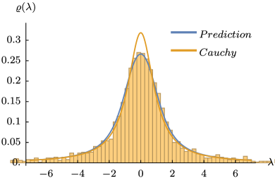
(a)

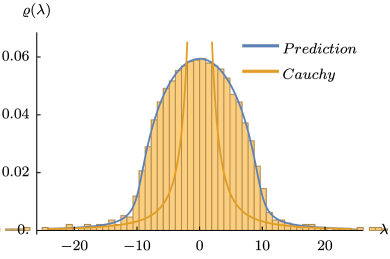
(b)

Figure 2: Distribution of the eigenvalues $\rho(\lambda)$ in the case in which $p_{a}(a)$ is the Cauchy distribution (see Section 2.4.1). We show a numerical check of Eq. 49 in the regime of (a) small $\eta$ (here $\eta=0.12$) and (b) large $\eta$ (here $\eta=11.7$). The histogram was built using $\mu=0$, $\omega=1$, $\gamma=1.1$ and $N=2000$, with $\nu=1$ in (a) and $\nu=10$ in (b).

2.4.1 Cauchy distributed $a_{i}$

Let us choose $p_{a}(a)$ to be a Lorentzian of width $\omega$ and centered at $\mu$,

$$p_{a}(a)=\frac{1}{\pi\omega}\left[\frac{\omega^{2}}{(a-\mu)^{2}+\omega^{2}}\right]\,.$$ (47)

Its characteristic function is an exponential, $\psi_{a}(z)=\exp(-i\mu z-\omega|z|)$, and then by using Eq. 37 we can compute $C(\lambda)$ in closed form:

$$C(\lambda)=\frac{1}{4}\left\{\omega+i(\lambda-\mu)\pm\sqrt{\left[\omega+i(\lambda-\mu)\right]^{2}+8\eta}\right\}\,.$$ (48)

We choose the branch with the minus sign for which $\real C(\lambda)\leq\omega/2$. Using Eq. 36 then yields

$$\rho(\lambda)=-\frac{\omega-\left\{4\omega^{2}(\lambda-\mu)^{2}+\left[8\eta+\omega^{2}-(\lambda-\mu)^{2}\right]^{2}\right\}^{1/4}\cos(\theta_{\lambda}/2)}{4\pi\eta}+\order{1/N}\,,$$ (49)

with

$$\theta_{\lambda}\equiv\arg\left\{\left[\omega+i(\lambda-\mu)\right]^{2}+8\eta\right\}\,.$$ (50)

In Fig. 2a we plot Eq. 49 against numerical results in the small-$\eta$ region: we find a good agreement with the theoretical prediction, as well as visible departures from the Cauchy distribution, especially in the bulk.

Another interesting limit is the one of large $\eta$, i.e., $\gamma=1$ and $\nu$ large. It has been shown in Krajenbrink_2021,Refs. Ref. [42] that, whenever $p_{a}(a)$ is rapidly decaying close to the edge of its finite support, then the spectral density $\rho(\lambda)$ interpolates between $p_{a}(a)$ and $\rho_{\text{GOE}}(\lambda)$ as the value of $\nu$ is increased. Note, however, that in the present case $p_{a}(a)$ decays algebraically and its support is not compact, so the outcome is less clear. The correct way of taking this limit is to rescale the eigenvalues as $\kappa\equiv\lambda/\sqrt{4\eta}$ and look for the distribution $\rho_{\kappa}(\kappa)=\sqrt{4\eta}\rho(\sqrt{4\eta}\kappa)$. From Eq. 48 we see that, if $\eta\gg\omega,\mu$, then

$$C(\sqrt{4\eta}\kappa)=\frac{\sqrt{\eta}}{2}\left[i\kappa-\sqrt{2-\kappa^{2}}\right]+\order{\eta^{0},1/N}\,,$$ (51)

and for large $N$ we get from Eq. 36 that $\rho_{\kappa}(\kappa)\to\rho_{\text{GOE}}(\kappa)$ (see Eq. 41). For large but finite $\eta$ and $N\to\infty$, on the other hand, the bulk distribution of $\kappa$ looks like a semicircle (as in the GOE ensemble), but with fat tails whose width grows with $\omega$ (see Fig. 3a). Moreover, the whole distribution shifts rigidly by changing its center $\mu/\sqrt{4\eta}$. Numerical results in the large-$\eta$ region are again nicely reproduced by Eq. 49, as shown in Fig. 2b.

Note that one can equivalently get to Eq. 48 by first computing the resolvent associated with the Lorentzian distribution in Eq. 47, i.e.,

$$\mathcal{G}_{\text{Cauchy}}(\lambda)=\frac{1}{\lambda-\mu\pm i\omega}\,,$$ (52)

where the $\pm$ branches correspond to $\Im{\lambda}>0$ or $\Im{\lambda}<0$, respectively. This can be obtained by explicitly performing the complex integral in Eq. 43, which only entails simple poles for a Cauchy distribution. One can then easily solve the self-consistency equation (42), which turns out to be quadratic, and thus recover Eq. 48.

(a)

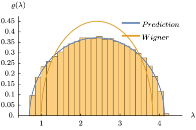
(b)

Figure 3: (a) Limiting distribution of the rescaled eigenvalues $\kappa=\lambda/\sqrt{4\eta}$, with $\rho(\lambda)$ given in Eq. 49 for the Cauchy case (see Section 2.4.1). In this plot we used $\mu=0$ and $\omega=0.5$. (b) Distribution of the eigenvalues $\rho(\lambda)$ in the case in which $p_{a}(a)$ is the Wigner semicircle distribution (see Section 2.4.2), and numerical check of the prediction in Eq. 56. The histogram was built using $r=\sqrt{2}$, $\mu=1+\sqrt{2}$, $\nu=1$, $\gamma=1.1$ and $N=2000$.

2.4.2 Wigner distributed $a_{i}$

Another simple case is the one in which $p_{a}(a)$ itself is chosen as the ($\mu$-centered) Wigner distribution

$$p_{a}(a)\equiv\frac{2}{\pi\sigma^{2}}\sqrt{\sigma^{2}-(a-\mu)^{2}}\,,$$ (53)

whose corresponding resolvent is

$$\mathcal{G}_{a}(z)=\frac{2}{\sigma^{2}}\left[z-\mu-\sqrt{(z-\mu)^{2}-\sigma^{2}}\right]\,.$$ (54)

The self-consistency equation (42) is again quadratic and it yields

$$C(\lambda)=2\eta\frac{i(\lambda-\mu)\pm\sqrt{\sigma^{2}+8\eta-(\lambda-\mu)^{2}}}{\sigma^{2}+8\eta}\,,$$ (55)

so that by choosing the branch with the minus sign and using Eq. 36 we find

$$\rho(\lambda)=\frac{2\sqrt{\sigma^{2}+8\eta-(\lambda-\mu)^{2}}}{\pi(\sigma^{2}+8\eta)}\Theta\left(\sigma^{2}+8\eta-(\lambda-\mu)^{2}\right)+\order{1/N}\,.$$ (56)

As expected, this is still a Wigner distribution centered in $\lambda=\mu$, but its width gets corrected as $\sigma^{2}\to\sigma^{2}+8\eta$.

2.5 Approximate solutions

For most choices of the diagonal disorder distribution $p_{a}(a)$, Eq. 37 cannot be solved exactly. However, since $\eta$ is a small parameter for large $N$ and $\gamma>1$ (which is the case we are mostly interested in), it may be sufficient to note that $C(\lambda)\sim\order{\eta}\sim\order{N^{1-\gamma}}$: this can be taken as a starting point for constructing self-consistent approximations for large $N$.

By expanding recursively the exponential in Eq. 37 and using that $C(\lambda)\sim\order{\eta}$, one gets

$$C(\lambda)= -\eta\int_{0}^{\infty}\differential{z}\psi_{a}(-z)e^{-i\lambda z}$$

$$+2\eta^{2}\int_{0}^{\infty}\differential{z}\int_{0}^{\infty}\differential{s}z\psi_{a}(-z)\psi_{a}(-s)e^{-i\lambda(z+s)}+\order{\eta^{3}}\,.$$ (57)

Note that

$$\real C(\lambda_{\varepsilon})=-\eta\,p_{a}(\lambda_{\varepsilon})+\order{\eta^{2}}\xrightarrow[\varepsilon\to 0]{N\gg 1}-\eta\,p_{a}(\lambda)\leq 0\,,$$ (58)

in such a way that $G(y)$ is indeed well-behaved at $y\to+\infty$, as we had assumed in Section 2.1. Plugging Eq. 57 into Eq. 36 now gives

$$\rho(\lambda)=p_{a}(\lambda)-\frac{2\eta}{\pi}\real\int_{0}^{\infty}\differential{z}\int_{0}^{\infty}\differential{s}z\psi_{a}(-z)\psi_{a}(-s)e^{-i\lambda(z+s)}+\order{\eta^{2},N^{-1}}\,.$$ (59)

Of course this approximation becomes meaningless if $\gamma\geq 2$, where the higher order corrections we neglected when we took the saddle-point approximation mingle with the $\mathcal{O}(\eta)$ correction.

Alternatively, one can expand the exponential in Eq. 37 as

$$C(\lambda)\simeq-\eta\int_{0}^{\infty}\differential{z}\psi_{a}(-z)e^{-i\lambda z}-2\eta C(\lambda)\int_{0}^{\infty}\differential{z}z\psi_{a}(-z)e^{-i\lambda}\,,$$ (60)

corresponding to a partial resummation of the perturbative series in $\eta$: this is the so-called self-consistent Hartree-Fock approximation [81]. From Eq. 60 we then obtain

$$C(\lambda)\simeq\frac{-\eta\int_{0}^{\infty}\differential{z}\psi_{a}(-z)e^{-i\lambda z}}{1+2\eta\Sigma(\lambda)}\,,$$ (61)

with the self-energy

$$\Sigma(\lambda)=\int_{0}^{\infty}\differential{z}z\psi_{a}(-z)e^{-i\lambda z}\,.$$ (62)

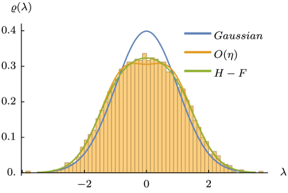
Figure 4: Distribution of the eigenvalues $\rho(\lambda)$ in the case in which $p_{a}(a)$ is Gaussian with unit variance, and $B$ is a GOE matrix as in Eq. 1. Numerical results are compared to the first $\order{\eta}$ correction given in Eq. 63, and to the Hartree-Fock approximation given in Eq. 61. The histogram was built using $N=2000$, $\nu=1$ and $\gamma=1.1$, corresponding to $\eta=0.12$.

An explicit example: the Gaussian case. We finally test both approximations in the case where $p_{a}(a)$ is chosen to be Gaussian (with zero mean and variance $\sigma^{2}$), as in the original Rosenzweig-Porter model [26]. By using $\psi_{a}(z)=\exp(-z^{2}\sigma^{2}/2)$ in Eq. 59, one finds

$$\rho(\lambda)=p_{a}(\lambda)+\sqrt{\frac{2}{\pi}}\frac{\eta}{\sigma^{3}}e^{-\lambda^{2}/(2\sigma^{2})}\left[\frac{2\sqrt{2}\lambda}{\sigma}F\left(\frac{\lambda}{\sqrt{2}\sigma}\right)-1\right]+\order{\eta^{2},N^{-1}}\,,$$ (63)

where $F(z)$ is the Dawson function defined as $F(z)\equiv e^{-z^{2}}\int_{0}^{z}e^{y^{2}}\differential{y}\,.$ The corrected spectral density is plotted in Fig. 4, and comparison with the eigenvalue spectrum computed numerically shows a fair agreement. Using instead the Hartree-Fock approximation for $C(\lambda)$ given in Eq. 61 results in a better agreement with the numerical data in the central region of the spectrum.

3 Number of eigenvalues in an interval and level compressibility

In this Section we consider the number of eigenvalues $I_{N}[\alpha,\beta]$ in a finite interval $[\alpha,\beta]$, as given by Eq. 10, and compute its cumulant generating function. This, in turn, can be used to access the level compressibility $\chi(E)$ defined in Eq. 11. As we explained in the Introduction, $\chi(E)$ represents a simple measure of the rigidity of the spectrum, which in turn allows us to distinguish between the phases of the model.

This program can be achieved by following the replica-based procedure introduced and exploited in Metz_2016,Metz_2017,Refs. Ref. [82, 83], which we briefly outline here. Starting from the definition of the spectral density in Eq. 9, we first rewrite Eq. 10 as

$$I_{N}[\alpha,\beta]=\sum_{i=1}^{N}\left[\Theta(\beta-\lambda_{i})-\Theta(\alpha-\lambda_{i})\right]\,.$$ (64)

Now we recall that the Heaviside function can be represented in terms of the discontinuity of the complex logarithm,

$$\Theta(-x)=\frac{1}{2\pi i}\lim_{\varepsilon\to 0^{+}}\left[\ln(x+i\varepsilon)-\ln(x-i\varepsilon)\right]\,,$$ (65)

so that we interpret

$$\sum_{i=1}^{N}\Theta(\alpha-\lambda_{i})=\frac{1}{2\pi i}\lim_{\varepsilon\to 0^{+}}\left[\ln\det(\mathcal{H}-\alpha_{\varepsilon}\mathbb{1})-\ln\det(\mathcal{H}-\alpha_{\varepsilon}^{*}\mathbb{1})\right]\,,$$ (66)

where we called as before $\alpha_{\varepsilon}\equiv\alpha-i\varepsilon$ with $\varepsilon>0$. This allows us to express $I_{N}[\alpha,\beta]$ in terms of the partition function given in Eq. 19, which leads to

$$I_{N}[\alpha,\beta]=-\frac{1}{\pi i}\lim_{\varepsilon\to 0^{+}}\ln\left[\frac{\mathcal{Z}(\beta_{\varepsilon})\mathcal{Z}(\alpha_{\varepsilon}^{*})}{\mathcal{Z}(\beta_{\varepsilon}^{*})\mathcal{Z}(\alpha_{\varepsilon})}\right]\,.$$ (67)

In order to compute the moments of $I_{N}$, we first address its cumulant generating function

$$\mathcal{F}_{[\alpha,\beta]}(s)\equiv\frac{1}{N}\ln\expectationvalue{e^{-sI_{N}[\alpha,\beta]}}=\frac{1}{N}\ln\langle e^{\frac{s}{\pi i}\lim_{\varepsilon\to 0^{+}}\ln\{{\mathcal{Z}}(\beta_{\epsilon}){\mathcal{Z}}(\alpha_{\epsilon}^{*})[{\mathcal{Z}}(\beta^{*}_{\epsilon}){\mathcal{Z}}(\alpha_{\epsilon})]^{-1}\}}\rangle\,.$$ (68)

Assuming now that one can move the limit $\varepsilon\to 0^{+}$ at the front of this expression, we obtain

$$\mathcal{F}_{[\alpha,\beta]}(s)=\lim_{\varepsilon\to 0^{+}}\frac{1}{N}\ln Q_{[\alpha,\beta]}(s)\,,$$ (69)

where we introduced

$$Q_{[\alpha,\beta]}(s)\equiv\expectationvalue{\left[\mathcal{Z}(\beta_{\varepsilon}^{*})\mathcal{Z}(\alpha_{\varepsilon})\right]^{is/\pi}\left[\mathcal{Z}(\beta_{\varepsilon})\mathcal{Z}(\alpha_{\varepsilon}^{*})\right]^{-is/\pi}}\,.$$ (70)

The latter can be accessed by first evaluating

$$Q_{[\alpha,\beta]}(n_{\pm})\equiv\expectationvalue{\left[\mathcal{Z}(\beta_{\varepsilon}^{*})\mathcal{Z}(\alpha_{\varepsilon})\right]^{n_{+}}\left[\mathcal{Z}(\beta_{\varepsilon})\mathcal{Z}(\alpha_{\varepsilon}^{*})\right]^{n_{-}}}$$ (71)

within the replica formalism with $n_{\pm}$ integer, and then performing its analytic continuation to

$$Q_{[\alpha,\beta]}(s)=\lim_{n_{\pm}\to\pm is/\pi}Q_{[\alpha,\beta]}(n_{\pm})\,.$$ (72)

To obtain the level compressibility in Eq. 11, we finally compute the cumulants

$$\frac{\kappa_{j}[\alpha,\beta]}{N}=(-1)^{j}\evaluated{\partial_{s}^{j}\mathcal{F}_{[\alpha,\beta]}(s)}_{s=0}\,,$$ (73)

and we evaluate them at $\alpha=-E$, $\beta=E$.

We remark that the average spectral density $\rho(E)$ is formally proportional to the derivative with respect to $E$ of the first cumulant $\kappa_{1}(E)=\left\langle\mathcal{I}[-E,E]\right\rangle$ (see Eq. 10), thus providing an alternative way to compute $\rho(E)$ which does not rely on the Edwards-Jones formula in Eq. 18.

3.1 Replica action and saddle-point equations

The details of this derivation are reported in Section D.1. In analogy with Section 2, here we express

$$Q_{[\alpha,\beta]}(n_{\pm})\propto \int\mathcal{D}(i\varphi)\,\exp{N\mathcal{S}_{n_{\pm}}[\varphi;\hat{\Lambda}]}\,,$$ (74)

$$\mathcal{S}_{n_{\pm}}[\varphi;\hat{\Lambda}]\equiv \frac{1}{2\eta}\int\differential{\vec{\tau}}\differential{\vec{\tau}^{\prime}}\varphi(\vec{\tau})M(\vec{\tau},\vec{\tau}^{\prime})\varphi(\vec{\tau}^{\prime})$$

$$+\ln\int\differential{\vec{\tau}}\exp[-\frac{i}{2}\vec{\tau}\,\hat{\Lambda}\,\vec{\tau}-\int\differential{\vec{\tau}^{\prime}}M(\vec{\tau},\vec{\tau}^{\prime})\varphi(\vec{\tau}^{\prime})]\,\psi_{a}\left(-\frac{1}{2}\vec{\tau}\,\hat{L}\,\vec{\tau}\right)\,,$$ (75)

where the replica vectors $\vec{\tau}\in\mathbb{R}^{n}$ live in dimension $n=2(n_{+}+n_{-})$. Each of the four replica sets corresponds to one sector in the block matrices

$$\hat{\Lambda}\equiv\matrixquantity(\alpha_{\varepsilon}\mathbb{1}_{n_{+}}&&&\\ &\bar{\beta}_{\varepsilon}\mathbb{1}_{n_{+}}&&\\ &&\beta_{\varepsilon}\mathbb{1}_{n_{-}}&\\ &&&\bar{\alpha}_{\varepsilon}\mathbb{1}_{n_{-}})\,,\;\;\;\qquad\hat{L}\equiv\matrixquantity(\mathbb{1}_{n_{+}}&&&\\ &-\mathbb{1}_{n_{+}}&&\\ &&\mathbb{1}_{n_{-}}&\\ &&&-\mathbb{1}_{n_{-}})\,,$$ (76)

where we called $\bar{\alpha}_{\varepsilon}=-\alpha^{*}_{\varepsilon}$, and similarly for $\bar{\beta}_{\epsilon}$. Finally, in Eq. 75 we introduced the function

$$M(\vec{\tau},\vec{\tau}^{\prime})\equiv\left(\vec{\tau}\,\hat{L}\,\vec{\tau}^{\prime}\right)^{2}\,,$$ (77)

while we recall that $\psi_{a}(z)$ was given in (32). Next, we need to compute the functional integration over $\mathcal{D}(i\varphi)$ in Eq. 74 in the limit of large $N$. From Eq. 75, the saddle-point equation follows simply as

$$\varphi_{0}(\vec{\tau})=\frac{\eta}{Z_{\varphi}}\exp[-\frac{i}{2}\vec{\tau}\,\hat{\Lambda}\,\vec{\tau}-\int\differential{\vec{\tau}^{\prime}}M(\vec{\tau},\vec{\tau}^{\prime})\varphi_{0}(\vec{\tau}^{\prime})]\,\psi_{a}\left(-\frac{1}{2}\vec{\tau}\,\hat{L}\,\vec{\tau}\right)\,,$$ (78)

with

$$Z_{\varphi}\equiv\int\differential{\vec{\tau}}\exp[-\frac{i}{2}\vec{\tau}\,\hat{\Lambda}\,\vec{\tau}-\int\differential{\vec{\tau}^{\prime}}M(\vec{\tau},\vec{\tau}^{\prime})\varphi_{0}(\vec{\tau}^{\prime})]\,\psi_{a}\left(-\frac{1}{2}\vec{\tau}\,\hat{L}\,\vec{\tau}\right)\,.$$ (79)

In order to better quantify the finite-size corrections and to make contact with the calculation performed in Metz_2017,Refs. Ref. [83] for the pure GOE case, in Section D.2 we also compute the Gaussian fluctuations around the saddle-point $\varphi_{0}(\vec{\tau})$, leading to

$$Q_{[\alpha,\beta]}(n_{\pm})=\exp{N\mathcal{S}_{n_{\pm}}[\varphi_{0};\hat{\Lambda}]+\frac{1}{2}\sum_{k=1}^{\infty}\frac{(-1)^{k}}{k}\Tr T^{k}}+\order{1/N^{2}}\,,$$ (80)

with

$$T(\vec{\tau}_{1},\vec{\tau}_{2})\equiv\varphi_{0}(\vec{\tau}_{1})\left[M(\vec{\tau}_{1},\vec{\tau}_{2})-\frac{1}{\eta}\int\differential{\vec{\tau}^{\prime}}M(\vec{\tau}_{2},\vec{\tau}^{\prime})\varphi_{0}(\vec{\tau}^{\prime})\right]\,.$$ (81)

Note that $\varphi_{0}(\overrightarrow{\mathbf{\tau}})\sim\order{\eta}$ (see Eq. 78), so that the function $T(\vec{\tau}_{1},\vec{\tau}_{2})$ itself is also of $\order{\eta}$.

3.2 Rotationally-invariant Ansatz

In the pure GOE case (which is recovered, for instance, by setting $\psi_{a}(z)=1$ identically in the expressions above), the saddle-point equation (78) suggests to look for a replica-symmetric solution in the form of a Gaussian, i.e.,

$$\varphi_{0}(\vec{\tau})=\mathcal{N}\exp(-\frac{1}{2}\vec{\tau}\,\hat{C}^{-1}\,\vec{\tau})\,,$$ (82)

where $\hat{C}$ is another block-diagonal matrix of the form

$$\hat{C}\equiv\matrixquantity(\Delta_{\alpha}\mathbb{1}_{n_{+}}&&&\\ &\bar{\Delta}_{\beta}\mathbb{1}_{n_{+}}&&\\ &&\Delta_{\beta}\mathbb{1}_{n_{-}}&\\ &&&\bar{\Delta}_{\alpha}\mathbb{1}_{n_{-}})\,.$$ (83)

The four parameters $\Delta_{\alpha},\bar{\Delta}_{\alpha},\Delta_{\beta}$ and $\bar{\Delta}_{\beta}$ and are to be fixed, together with the prefactor $\mathcal{N}$ in Eq. 82, by substituting the Ansatz in Eq. 82 back into the saddle-point equation (78).

This strategy has proven effective in Metz_2017,Refs. Ref. [83] and, for completeness, in Appendix E we sketch the entire calculation for the GOE case. However, in the presence of a nontrivial $\psi_{a}(z)$ in Eq. 78, there is no reason why the Ansatz in Eq. 82 should work: the structure of Eq. 78 suggests instead to extend it to the form

$$\varphi_{0}(\vec{\tau})=\mathcal{N}\exp(-\frac{1}{2}\vec{\tau}\,\hat{C}^{-1}\,\vec{\tau})\psi_{a}\left(-\frac{1}{2}\vec{\tau}\,\hat{L}\,\vec{\tau}\right)\,.$$ (84)

This can be plugged into Eq. 78 to first obtain $\mathcal{N}=\eta/Z_{\varphi}$, where

$$Z_{\varphi}=\int\differential{\vec{\tau}}\varphi_{0}(\vec{\tau})\,.$$ (85)

By using Gaussian integration one can then show that

$$\int\differential{\vec{\tau}^{\prime}}M(\vec{\tau},\vec{\tau}^{\prime})\varphi_{0}(\vec{\tau}^{\prime})=\eta\vec{\tau}\,\hat{K}\,\vec{\tau}\,,$$ (86)

where $\hat{K}$ is a diagonal matrix given by

$$\hat{K}=-i\hat{L}\,\mathcal{G}_{a}\left((i\hat{L}\hat{C})^{-1}\right)\,,$$ (87)

$\mathcal{G}_{a}$ is the resolvent in Eq. 43, and $\hat{L}$ is given in Eq. 76. The remaining free parameters in Eq. 82 can be determined by solving the set of four self-consistency equations which follow from Eq. 78, i.e.,

$$\hat{C}^{-1}\,=2\eta\,\hat{K}+i\,\hat{\Lambda}\,.$$ (88)

Finally, both the action and its Gaussian fluctuation matrix $T$ (see Eq. 81) can be computed by using the saddle-point solution in Eq. 84. First, notice that the action in Eq. 75 takes the form

$$\mathcal{S}_{n_{\pm}}[\varphi_{0};\hat{\Lambda}] =\frac{1}{2}\int\differential{\vec{\tau}}\left(\vec{\tau}\,\hat{K}\,\vec{\tau}\right)\varphi_{0}(\vec{\tau})+\ln Z_{\varphi}$$

$$=\frac{\eta}{2}\sum_{i}K_{ii}^{2}+\ln\int_{-\infty}^{\infty}\differential{a}p_{a}(a)\exp{-\frac{1}{2}\Tr\ln[(i\hat{L}\hat{C})^{-1}-a]}+\text{const.}\,.$$ (89)

The constant term vanishes upon taking the analytic continuation $n_{\pm}\to\pm is/\pi$, yielding

$$\mathcal{S}_{\pm\frac{is}{\pi}}[\varphi_{0};\hat{\Lambda}]= \frac{is\eta}{2\pi}\left(k_{\alpha}^{2}+\bar{k}_{\beta}^{2}-k_{\beta}^{2}-\bar{k}_{\alpha}^{2}\right)$$

$$+\ln\int_{-\infty}^{\infty}\differential{a}p_{a}(a)\exp{-\frac{is}{2\pi}\ln\left[\frac{(\bar{\Delta}_{\beta}^{-1}+ia)(\Delta_{\alpha}^{-1}-ia)}{(\bar{\Delta}_{\alpha}^{-1}+ia)(\Delta_{\beta}^{-1}-ia)}\right]}\,,$$ (90)

where we introduced for brevity $\hat{K}\equiv\text{diag}(k_{\alpha}\mathbb{1}_{n_{+}},\bar{k}_{\beta}\mathbb{1}_{n_{+}},k_{\beta}\mathbb{1}_{n_{-}},\bar{k}_{\alpha}\mathbb{1}_{n_{-}})$. Note that this action coincides at leading order with the cumulant generating function in Eq. 69, i.e.,

$$\mathcal{F}_{[\alpha,\beta]}(s)=\lim_{\varepsilon\to 0^{+}}\mathcal{S}_{\pm\frac{is}{\pi}}[\varphi_{0};\hat{\Lambda}]+\order{\eta/N}\,,$$ (91)

where we used Eq. 80 (the estimate of the large-$N$ correction will soon be justified). In the next Section we will make this result more explicit in the case of an interval which is symmetric around the origin.

The Gaussian fluctuations around the saddle-point are studied in Section D.2. A closed-form result is not available in this case (in contrast to the GOE case, see Appendix E), because the calculation involves increasingly complex generalizations of the resolvent $\mathcal{G}_{a}(z)$ which encode higher order correlations (see Eq. D.18). However, we can show that the Gaussian fluctuations add to the leading order term in Eq. 91 a correction of $\order{\eta/N}=\order{N^{-\gamma}}$, which is strongly suppressed for large $N$ in the region $\gamma>1$ which we focus on here.

3.3 General result in the case of a symmetric interval

We consider now the simpler case in which $\alpha=-E$ and $\beta=E$, and we take a symmetric distribution $p_{a}(a)$. From Eqs. 87 and 88 one can deduce that the entries of the matrix $\hat{C}$ are related by the following symmetries:

$$\Delta_{\alpha}\equiv\Delta\equiv re^{i\theta}\,,\;\;\;\;\;\bar{\Delta}_{\alpha}=\Delta_{\alpha}^{*}=\Delta_{\beta}\,,\;\;\;\;\;\bar{\Delta}_{\beta}=\Delta_{\beta}^{*}\,.$$ (92)

The same holds for the entries of $\hat{K}$ (see Eq. 87), hence we will simply call $k_{\alpha}\equiv k$. The problem is then reduced to computing one single unknown, namely $\Delta$: from Eqs. 87 and 88, this amounts to solving the self-consistency equations

$$\begin{dcases}\Delta^{-1}=\varepsilon-iE+2\eta k\,,\\ k=-i\mathcal{G}_{a}\left(-i\Delta^{-1}\right)\,.\end{dcases}$$ (93)

The action in Eq. 90 then takes the form

$$\mathcal{S}[\varphi_{0};\hat{\Lambda}]=-\frac{2\eta s}{\pi}\Im{k^{2}}+\ln\int_{-\infty}^{\infty}\differential{a}p_{a}(a)\exp[-\frac{s}{\pi}\arctan\left(\frac{\sin 2\theta}{a^{2}r^{2}+\cos 2\theta}\right)]\,,$$ (94)

where the branch of the $\arctan$ is chosen so that it returns an angle in $[0,\pi]$. From Eq. 69 we can then read the leading order contribution to the rate function, namely

$$\mathcal{F}_{[-E,E]}(s)=\mathcal{S}[\varphi_{0};\hat{\Lambda}]+\order{\eta/N}=-ms+\ln\expectationvalue{e^{-sf(a)}}_{a}+\order{\eta/N}\,.$$ (95)

Here we used the notation $\expectationvalue{\bullet}_{a}$ to indicate the average over $p_{a}(a)$, and we introduced for brevity

$$m \equiv\frac{2\eta}{\pi}\Im{k^{2}}=-\frac{2\eta}{\pi}\imaginary\left[\mathcal{G}_{a}\left(-i\Delta^{-1}\right)\right]^{2}\,,$$ (96)

$$f(a) \equiv\frac{1}{\pi}\arctan\left(\frac{\sin 2\theta}{a^{2}r^{2}+\cos 2\theta}\right)\in[0,1]\,,$$ (97)

where in the first line we used Eq. 93. The cumulant generating function in Eq. 95, together with the self-consistency equations (93), represent our second main result. As we stressed above, when $\eta$ is given by Eq. 2, the correction to Eq. 95 is of $\order{\eta/N}=\order{N^{-\gamma}}$, which is strongly suppressed for large $N$ in the region $\gamma>1$.

Expanding Eq. 95 in powers of $s$ we get

$$\mathcal{F}_{[-E,E]}(s)\simeq-s\left[m+\expectationvalue{f(a)}_{a}\right]+\frac{s^{2}}{2}\left[\expectationvalue{f^{2}(a)}_{a}-\expectationvalue{f(a)}_{a}^{2}\right]+\order{s^{3},\eta/N}\,,$$ (98)

and by comparison with Eq. 73 we can identify the first two cumulants

$$\frac{\kappa_{1}}{N} =m+\expectationvalue{f(a)}_{a}+\order{\eta/N}\,,$$ (99)

$$\frac{\kappa_{2}}{N} =\expectationvalue{f^{2}(a)}_{a}-\expectationvalue{f(a)}_{a}^{2}+\order{\eta/N}\,.$$ (100)

From Eq. 11, we finally obtain the level compressibility

$$\chi(E)=\frac{\expectationvalue{f^{2}(a)}_{a}-\expectationvalue{f(a)}_{a}^{2}}{m+\expectationvalue{f(a)}_{a}}+\order{\eta/N}\,.$$ (101)

We remark that not only the level compressibility, but actually all the moments of $I_{N}[-E,E]$ can be simply computed starting from Eq. (95): they read (at leading order for large $N$)

$$\langle(I_{N}[-E,E])^{m}\rangle\simeq N\langle[f(a)]^{m}\rangle_{a}\,,\quad m\geq 2\;.$$ (102)

3.3.1 Limit of a pure diagonal matrix with random i.i.d. entries

It is instructive, at this point, to consider the limit $\eta\to 0$. In this case the GOE part of Eq. 1 is neglected, and the spectral properties are completely determined by the matrix $A$, whose entries are independent and identically distributed according to $p_{a}(a)$. The self-consistency equation (88) then reduces to

$$\hat{C}\,=(i\,\hat{\Lambda})^{-1}\,,$$ (103)

whence

$$\Delta=\evaluated{\Delta_{\alpha}}_{\alpha=-E}=\frac{iE+\varepsilon}{E^{2}+\varepsilon^{2}}\equiv re^{i\theta}\,,$$ (104)

and there is no need to determine the entries of $\hat{K}$ since it does not enter the expression of the saddle-point action (94) for $\eta=0$. From Eq. 94 we obtain, for $\varepsilon\to 0^{+}$,

$$\mathcal{S}[\varphi_{0};\hat{\Lambda}] =\ln\int_{-\infty}^{\infty}\differential{a}p_{a}(a)\exp{-\frac{s}{\pi}\arctan\left[\frac{0^{+}}{(a/E)^{2}-1}\right]}$$

$$=\ln\left[1+(e^{-s}-1)\int_{-E}^{E}\differential{a}p_{a}(a)\right]\,,$$ (105)

where we used that the branch of $\arctan(z)\in[0,\pi]$ has a discontinuity in $z=0$, i.e., it jumps from $\pi$ to $0$ as $z$ becomes positive. From Eqs. 95 and 10, we can then read out the cumulant generating function

$$\mathcal{F}_{[-E,E]}(s)=\ln\left[1+(e^{-s}-1)\frac{\expectationvalue*{I_{N}[-E,E]}_{a}}{N}\right]\,.$$ (106)

In this way we recover the standard textbook result for the cumulant generating function in the case of i.i.d. random variables, which we sketch for completeness in Appendix A. In particular, the level compressibility in Eq. 11 reads in this case

$$\chi(E)=1-\frac{\expectationvalue{I_{N}[-E,E]}_{a}}{N}\,,$$ (107)

so that in general $\chi(E)\sim 1$ for small $E$, and $\chi(E)\to 0$ for large $E$.

Finally, we note that Eq. 106 is exact, because we have stressed above that the Gaussian fluctuations around the saddle-point are at least of $\order{\eta}$ and so they vanish in the limit $\eta\to 0$.

3.3.2 Limit of a pure GOE matrix

The opposite limit in which $A$ is neglected in Eq. 1 is obtained by setting $p_{a}(a)=\delta(a)$, whose corresponding resolvent is $\mathcal{G}_{a}(z)=1/z$ (indeed, summing zeros to the matrix $B$ in Eq. 1 does not change its spectrum). Equation (87) then implies $\hat{K}=\hat{C}$, where we used $\hat{L}^{2}=\mathbb{1}$ (see Eq. 76). The self-consistency equations (88) are then seen to coincide with Eq. E.2, corresponding to the GOE case studied in Metz_2017,Refs. Ref. [83] and here revisited in Appendix E. From Eq. 94 we obtain, in terms of $r$ and $\theta$ introduced in Eq. 92,

$$\mathcal{S}[\varphi_{0};\hat{\Lambda}]=-\frac{2\eta r^{2}s}{\pi}\sin 2\theta-\frac{2s\theta}{\pi}\,,$$ (108)

which is linear in $s$: we deduce that the cumulants higher than the average $\expectationvalue{I_{N}[-E,E]}$ are subleading for large $N$, and they are only accessible by explicitly computing the Gaussian fluctuations around the saddle-point (see Section D.2). Still, the leading order term in the first cumulant (see Eq. E.16) is correctly reproduced by Eq. 108.

3.4 Exactly solvable cases

The cumulant generating function we found in Eq. 95 is formal, in that $\Delta=re^{i\theta}$ must first be determined by solving the self-consistency equation (88). In the following, we will present two cases in which the result can be expressed in closed form, namely those in which $p_{a}(a)$ is the Cauchy or the Wigner distribution, respectively. While the former presents fat tails and is thus slowly decaying, the latter has a compact support and a well-defined edge.

3.4.1 Cauchy distributed $a_{i}$

Let us start from the case in which $p_{a}(a)$ is the Cauchy distribution, see Eq. 47. We set $\mu=0$, so that the problem remains symmetric around the origin. Using the expression of $\mathcal{G}_{a}(z)$ in Eq. 52, $\hat{K}$ in Eq. 87 reduces to

$$\hat{K}=\frac{\hat{C}}{1+\omega\hat{C}}\,.$$ (109)

Solving the self-consistency equation (88) then yields

$$\Delta=\evaluated{\Delta_{\alpha}}_{\alpha=-E}=2\left[\varepsilon-iE-\omega+\sqrt{8\eta+\left(\varepsilon-iE+\omega\right)^{2}}\right]^{-1}\equiv re^{i\theta}\,,$$ (110)

where we chose the positive branch of the square root so that $\real\Delta_{\alpha}>0$. After this choice, the constant $\varepsilon$ can be safely sent to zero. The resulting cumulant generating function is given in Eq. 95, where the averages are taken over the Cauchy distribution in Eq. 47, and the coefficient of the term linear in $s$ reads

$$m=\frac{4\eta r^{2}\sin\theta\left(r\omega+\cos\theta\right)}{\pi\left[1+(r\omega)^{2}+2r\omega\cos\theta\right]^{2}}\,.$$ (111)

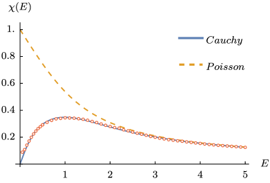
(a)

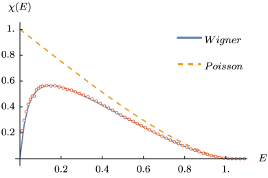
(b)

Figure 5: Numerical check of the level compressibility $\chi(E)$ predicted in Eq. 101 (solid blue line), for the case in which the elements of the diagonal matrix $A$ belong to the (a) Cauchy, or (b) Wigner distribution. Numerical data (symbols) are obtained from the numerical diagonalization of $N_{\text{tot}}=1000$ random matrices of size $N=5000$. The (dashed yellow) line denoted by Poisson shows the level compressibility as it would be in the absence of level repulsion – see the main text. In both plots we used the parameters $\mu=0$, $\gamma=1.1$. In (a) we chose $\omega=1$ and $\nu=1$, corresponding to $\eta=0.125$, while in (b) we set $\sigma=1$ and $\nu=0.2$, yielding $\eta=0.005$.

The resulting level compressibility $\chi(E)$ (see Eq. 101) is plotted in Fig. 5a, and it is compared to numerical results showing excellent agreement. We show in the same plot the level compressibility under the hypothesis that the level statistics is of the Poisson type, i.e., that the energy levels do not repel each other. This is given by Eq. 107 upon interpreting the average $\expectationvalue{\bullet}$ as taken over the average eigenvalue density $\rho(\lambda)$ for the case in which the matrix $A$ has Cauchy-distributed entries: this has been found previously in Eq. 49. Even for very small values of $\eta$, the behavior at low energies $E$ of the compressibility $\chi(E)$ is qualitatively very different: in the Poisson case we have $\chi(E)\sim 1$, while in the GRP model it is $\chi(E)\sim 0$. The latter $\chi(E)$ increases up to a maximum, whose position $E_{\text{max}}(\eta)$ grows monotonically (and sublinearly) with $\eta$.

3.4.2 Wigner distributed $a_{i}$

Let us now consider the case in which $p_{a}(a)$ is the Wigner distribution, see Eq. 53. Again we set $\mu=0$, so that the problem remains symmetric around the origin. Using the expression of $\mathcal{G}_{a}(z)$ in Eq. 54, the quantity $\hat{K}$ in Eq. 87 becomes

$$\hat{K}=-\frac{2}{\sigma^{2}\hat{C}}\left[1-\sqrt{1+(\sigma\hat{C})^{2}}\right]\,.$$ (112)

Solving the self-consistency equation (88) yields, after choosing the positive branch of the square root so that $\real\Delta_{\alpha}>0$ and letting $\varepsilon\to 0$,

$$\Delta=\evaluated{\Delta_{\alpha}}_{\alpha=-E}=\frac{iE(\sigma^{2}+4\eta)+4\eta\sqrt{\sigma^{2}+8\eta-E^{2}}}{16\eta^{2}+\sigma^{2}E^{2}}\equiv re^{i\theta}\,.$$ (113)

The resulting cumulant generating function is again given in Eq. 95, where the averages are taken over the Wigner distribution in Eq. 53. The analytical expression of the quantity $m$ in Eq. 96 is cumbersome, but it follows readily from Eq. 112. In Fig. 5b we plot the level compressibility $\chi(E)$ as we did for the Cauchy case, finding a qualitatively similar behavior.

3.5 Scaling limit and Thouless energy

In this Section we focus on the limit in which $E=x\eta^{\delta}$ and $\eta\ll 1$, while $x\sim\order{1}$. We can envision a different behavior depending on whether the exponent $\delta>1$, $\delta<1$ or $\delta=1$. The latter case turns out to be particularly interesting: we will show that the level compressibility computed in $\chi(E=x\eta^{\delta})$ assumes for $\delta=1$ a universal scaling form, which is independent of the particular choice of the distribution $p_{a}(a)$ of the entries of the diagonal matrix $A$.

To this end, let us go back to the self-consistency equations (93), which we can rewrite for $\delta=1$ and $\eta\ll 1$ as

$$\Delta^{-1} =\varepsilon-ix\eta-2i\eta\mathcal{G}_{a}\left(-i\Delta^{-1}\right)$$

$$\simeq\varepsilon-ix\eta-2i\eta\mathcal{G}_{a}\left(-i\varepsilon+\order{\eta}\right)\,,$$ (114)

where again $\Delta=re^{i\theta}$. By taking the complex conjugate of Eq. 114 and by summing and subtracting the two equations, we obtain the two conditions

$$r^{-1}\cos\theta =\varepsilon+2\eta\imaginary\mathcal{G}_{a}\left(-i\varepsilon+\order{\eta}\right)\xrightarrow[\varepsilon\to 0^{+}]{\eta\ll 1}2\pi\eta p_{a}(0)\,,$$ (115)

$$r^{-1}\sin\theta =x\eta+2\eta\real\mathcal{G}_{a}\left(-i\varepsilon+\order{\eta}\right)\xrightarrow[\varepsilon\to 0^{+}]{\eta\ll 1}x\eta\,,$$ (116)

where we used the Plemelj-Sokhotski formula recalled in Eq. 16, and the fact that for a symmetric distribution $p_{a}(a)$ one has

$$\principalvalue{\int\differential{a}\frac{p_{a}(a)}{a}}=0\,.$$ (117)

One then easily obtains, at leading order for small $\eta$ (and with $x=E/\eta$),

$$\tan\theta \simeq\frac{x}{2\pi p_{a}(0)}\equiv y\,,$$ (118)

$$r^{-1} \simeq 2\pi\eta p_{a}(0)\sqrt{1+y^{2}}\,.$$ (119)

Note that these manipulations are only possible under the additional assumption that the distribution $p_{a}(a)$ behaves regularly close to $a=0$, and that $p_{a}(0)\neq 0$.

We can now estimate the level compressibility in this limit. First, notice that

$$\mathcal{G}_{a}(-i\Delta^{-1})=i\pi p_{a}(0)+\order{\eta}\,,$$ (120)

so that from Eq. 96 we read

$$m=-\frac{2\eta}{\pi}\imaginary\left[\mathcal{G}_{a}(-i\Delta^{-1})\right]^{2}=\order{\eta^{2}}\,.$$ (121)

From Eq. 99, the first cumulant $\kappa_{1}$ thus reduces to

$$\frac{\kappa_{1}}{N} \simeq\expectationvalue{f(a)}_{a}=\int\differential{a}p_{a}(a)f(a)\simeq\frac{p_{a}(0)}{r}\int_{-\infty}^{\infty}\differential{u}f(u/r)$$

$$=\frac{p_{a}(0)}{r}\frac{2y}{\sqrt{1+y^{2}}}=2p_{a}(0)x\eta\,,$$ (122)

where in the first line we changed variable to $u=ra$ and we used the fact that $r^{-1}\sim\order{\eta}$ (see Eq. 119), while in the second line we explicitly computed the integral

$$\frac{1}{\pi}\int_{0}^{\infty}\differential{u}\arctan\left(\frac{\sin 2\theta}{u^{2}+\cos 2\theta}\right)=\frac{\tan\theta}{\sqrt{1+\tan^{2}\theta}}=\sin{\theta}\,,\;\;\;\;\;\;\;\theta\in\left[0,\frac{\pi}{2}\right]\,,$$ (123)

and we inserted the expression for $r$ found in Eq. 119 (note that $f(u/r)$ is actually $r$-independent – see Eq. 97). One could alternatively compute $\kappa_{1}$ by taking the average of Eq. 10: this leads to the same result upon expanding for small $E$ and $\eta$, since

$$\rho(\lambda)=p_{a}(\lambda)+\order{\eta}\,.$$ (124)

The same steps can be repeated for the second (and possibly any other) cumulant $\kappa_{2}$, yielding

$$\frac{\kappa_{2}}{N}\simeq\expectationvalue{f^{2}(a)}_{a}\simeq\frac{p_{a}(0)}{r}\int_{-\infty}^{\infty}\differential{u}f^{2}(u/r)\,.$$ (125)

From Eq. 101 we thus obtain the leading order estimate for the level compressibility when $\eta\ll 1$, which takes the universal scaling form

$$\chi(E) \simeq \chi_{T}\left(y=\frac{E}{2\pi p_{a}(0)\eta}\right)\,,$$

$$\chi_{T}(y) \equiv \frac{\sqrt{1+y^{2}}}{\pi^{2}y}\int_{0}^{\infty}\differential{u}\left\{\arctan\left[\frac{2y}{u^{2}(1+y^{2})+1-y^{2}}\right]\right\}^{2},$$ (126)

where we stress that we have chosen the branch $\arctan(z)\in[0,\pi]$. Upon integrating by parts and performing some algebra [86, 87], the integral over $u$ can be computed explicitly to give

$$\chi_{T}(y)=\frac{1}{\pi y}\left[2y\arctan(y)-\ln(1+y^{2})\right]\,.$$ (127)

The function $\chi_{T}(y)$ grows monotonically from $0$ to $1$ as we increase $y$, and it is plotted in Fig. 6a together with the level compressibility for the two cases explicitly solved above, i.e., Cauchy and Wigner. We find a good agreement at low energies $y$, while we observe a departure at large energies: here the scaling prediction keeps growing, while the actual compressibility must hit a maximum and start decreasing – see Fig. 5. The same trend can be observed in Fig. 6b, where we evaluate the level compressibility for different values of $\eta$, and show that they collapse on a common master curve when they are plotted as a function of $y\propto E/\eta$.

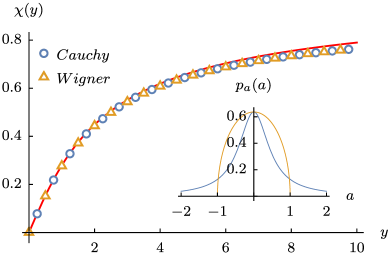
(a)

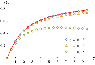
(b)

Figure 6: Scaling form of the level compressibility, in the limit in which $E\propto y\eta$ and $\eta\ll 1$. In (a) we compare the universal prediction in Eq. 127 (solid red line) with the two exactly solvable cases studied in Section 3.4 (symbols), showing a good agreement at low energies $y=E/[2\pi p_{a}(0)\eta]$ (i.e., the condition under which Eq. 127 was derived). We chose $\eta=5\cdot 10^{-4}$ and $\omega=0.5$, $\sigma=1$, so that $p_{a}(0)$ assumes the same value for the two distributions (see inset). In (b) we exemplify in the Cauchy case how the curves corresponding to different values of $\eta$ collapse onto the same master curve, when plotted as a function of $y\propto E/\eta$ for $\eta\ll 1$.

The other two cases ($\delta>1$ or $\delta<1$) can be easily addressed by the same token. When $\delta>1$, by studying the self-consistency equations as in Eq. 114 we obtain at leading order

$$\tan\theta\simeq y\eta^{\delta-1}\,,$$ (128)

$$r^{-1}\simeq 2\pi\eta p_{a}(0)\,.$$ (129)

It can be readily seen that $\kappa_{1}/N\simeq 2p_{a}(0)x\eta^{\delta}$ and $\kappa_{2}/N\sim\order{\eta^{2\delta-1}}$, so that in this limit

$$\chi(E=x\eta^{\delta})\sim\order{\eta^{\delta-1}}\,,\;\;\;\;\;\;\;\delta>1\,,\;\eta\ll 1\,.$$ (130)

This resembles the behavior of $\chi(E)$ in the case of a pure GOE matrix, see Sections 3.3.2 and E. Conversely, for $\delta<1$ the self-consistency equations (93) reduce to

$$\Delta^{-1}\simeq\varepsilon-ix\eta^{\delta}\,,$$ (131)

and, by comparison with Eq. 103, we identify this limit as that in which the eigenvalues behave as i.i.d. random variables. In particular (compare with Eq. 107),

$$\chi(E=x\eta^{\delta})\simeq 1-\frac{\expectationvalue{I_{N}[-E,E]}_{a}}{N}\,,\;\;\;\;\;\;\;\delta<1\,,\;\eta\ll 1\,.$$ (132)

The above analysis suggests to interpret the quantity $E_{T}\sim 2\pi p_{a}(0)\eta$ as the Thouless energy of the system. Indeed, consider again the limit in which $\eta\ll 1$, and let $E\propto\eta^{\delta}$. For $E\ll E_{T}$ (i.e., $\delta>1$), the eigenvalues organize in multiplets (or mini-bands [27]) and they repel each other as in the GOE ensemble – as a result, the level compressibility is zero at leading order (see Eq. 130). For $E\gg E_{T}$ ($\delta<1$), on the other hand, the various multiplets no longer interact, and we recover the Poisson statistics – see Eq. 132. Finally, the case $\delta=1$ marks a crossover in which the level compressibility $\chi(E/E_{T})$ assumes the universal scaling form given in Eq. 127. Indeed, the asymptotics of the function $\chi_{T}(y)$ in Eq. 127 can be checked to give

$$\chi_{T}(y)\simeq\begin{dcases}\frac{y}{\pi}\,,&y\ll 1\,,\\ 1-\frac{2(1+\ln y)}{\pi y}\,,&y\gg 1\,,\end{dcases}$$ (133)

showing that $\chi_{T}(y)$ interpolates between Wigner-Dyson statistics at low energy, and Poisson statistics at higher energy.

We finally note that a close relative of the level compressibility, namely the two-level spectral correlation function $C(t,t^{\prime})$ – see Eqs. (F.1)-(F.3) for its definition – was computed in Kravtsov_2015,Refs. Ref. [27] for the Hermitian GRP model. In the latter, the GOE matrix $B$ in Eq. 1 is replaced by a GUE matrix with complex entries, so that additional analytical techniques (notably the Harish-Chandra-Itzykson-Zuber integral [88]) are available. In particular, $C(t,t^{\prime})$ is shown in Kravtsov_2015,Refs. Ref. [27] to assume a universal scaling form within the fractal region $1<\gamma<2$, and for large $N$. In Appendix F we show that the corresponding scaling form of the level compressibility coincides, in the crossover regime in which $E\sim E_{T}$, with $\chi_{T}(y)$ in Eq. 127. This is quite remarkable, since these are in fact two distinct random matrix ensembles – and indeed their level compressibilities do not coincide for $E\gg E_{T}$ or $E\ll E_{T}$. This identification suggests that $\chi_{T}(y)$ originates from the structural properties of the model, rather than from the specific choice of the matrix $B$ (e.g., GOE, GUE, but also possibly Wishart or sparse random matrices).

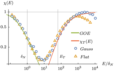
(a)

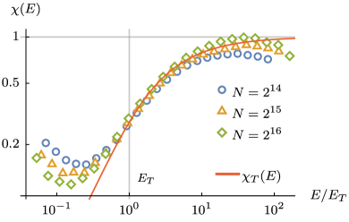
(b)

Figure 7: Behavior of the level compressibility $\chi(E)$ at low energies. The symbols correspond to numerical results, and we indicated with vertical lines the mean level spacing $\delta_{N}$ (see Eq. 4) and the Thouless energy $E_{T}\sim N^{1-\gamma}$. In panel (a), $p_{a}(a)$ is chosen Gaussian with unit variance or uniform, and $N=2^{16}$. The region $E\lesssim\delta_{N}$ is described by the GOE prediction in Eq. E.25, while the crossover region $E\sim E_{T}$ is described by the universal scaling form in Eq. 127. In panel (b), $p_{a}(a)$ is Gaussian, and we show the approach to the universal curve $\chi_{T}(E)$ for increasing values of the matrix size $N$. We used $\gamma=1.5$ throughout, and the simulations with $N=2^{14},2^{15},$ or $2^{16}$ are averaged over $N_{\text{tot}}=256,64,$ or $32$ samples, respectively.

3.6 Behavior for small $E$

In this final Section we use extensive numerical exact diagonalization of large random matrices in order to inspect the low-energy behavior of the level compressibility $\chi(E)$. Indeed, our prediction of Section 3.5 is expected to break down for energies of the order of the mean level spacing $\delta_{N}$ of the finite-sized matrix $\mathcal{H}$, which is given by $\delta_{N}\simeq[Np_{a}(0)]^{-1}$, Eq. (4). Equivalently, we expect that the leading order term in the saddle-point approximation adopted in our replica calculation (see Eqs. 69 and 80) provides the correct result in the $N\to\infty$ limit, while for a matrix of size $N$ and for sufficiently small $E$ we should eventually recover the exact GOE result $\chi_{\text{GOE}}(E)$ [89, 90, 88, 91, 78, 92, 93, 94], whose derivation is reported in Section E.3 – see Eq. E.25. The overall picture is thus the one we present in Fig. 7, and which we support by numerical results. The region $E\lesssim\delta_{N}$ is described by the GOE prediction in Eq. E.25. For $1<\gamma<2$ the Thouless energy $E_{T}\sim N^{1-\gamma}$ is such that $\delta_{N}\ll E_{T}\ll 1$, so that the crossover region with $E\sim E_{T}$ is described by the universal function $\chi_{T}(E)$ given in Eq. 127. For larger $E\gtrsim\order{1}$, the level compressibility becomes model-dependent and it is described by Eq. 101 (see also Fig. 5).

The datapoints presented in panel (a) of Fig. 7 correspond to the choices of $p_{a}(a)$ Gaussian or uniform, which supports our claim of universality of $\chi_{T}(E)$ in the region $E\sim E_{T}$. Note, in fact, that the data follow the predicted curves (up to finite-size effects) with no adjustable parameters (i.e., no fitting was needed). The datapoints are eventually observed to deviate from the scaling prediction, as they reach a maximum in correspondence of $E_{\text{max}}(\eta)\gg E_{\text{T}}$ and start decaying to zero as in Fig. 5. By increasing $N$, however, this maximum is observed to shift towards larger values of $E$, and the plateau around $\chi(E)\sim 1$ broadens accordingly.

4 Conclusions

In this work we used the replica method to study the average spectral density (Section 2) and the local level statistics (Section 3) of a deformed GOE random matrix ensemble known as the generalized RP model. We focused on its fractal intermediate phase with $1<\gamma<2$ [27], which is conveniently characterized in terms of the level compressibility $\chi(E)$ (see Eq. 11). We showed that $\chi(E)$ assumes a universal form $\chi_{T}(E/E_{T})$ independently of the character $p_{a}(a)$ of the deformation matrix $A$ (see Eq. 1), provided that the system is probed over energy scales of the order of the Thouless energy $E_{T}$ (see Section 3.5).

It is natural to conjecture that this universal regime should persist in structurally similar random matrix ensembles (even more so, since we showed that the same scaling function $\chi_{T}(y)$ can be recovered for the Hermitian GRP model – see Appendix F). For instance, one could numerically inspect the case in which the GOE matrix is replaced by a Wigner matrix (i.e., any real symmetric matrix with i.i.d. random entries taken from a probability distribution with finite variance), whose limiting average spectral density is still given by the semi-circle law [95]. Similarly, it would be interesting to study the effect of the diagonal deformation matrix $A$ on a Wishart matrix [96], or else on a sparse (rather than dense) matrix $B$, such as those describing the Erdös-Rényi random graph [97, 98, 99], which can still be treated analytically (at least to some extent); if the average connectivity is chosen to be finite, the spectral density of Erdös-Rényi is no longer a semi-circle, but the local statistics is still of the Wigner-Dyson type.

Along our derivation, we heavily relied on the independence of the elements $a_{i}$ characterizing the diagonal disorder (as usually assumed in standard formulations of the GRP model). However, the introduction of short-ranged correlations between the levels $a_{i}$ seems within reach of the replica method. In particular, the analysis of DeTomasi_2022,Refs. Ref. [100] suggests that changing the power $d$ at which the distance between sorted diagonal elements $a_{n}<a_{n+1}$ grows, e.g., $(a_{n+k}-a_{n})\propto k^{d}$, has important implications on the phase diagram. Moreover, in Section 3.5 we assumed a regular character of $p_{a}(a)$ in correspondence of $a\to 0$, while it would be interesting to check the fate of the universal scaling form $\chi_{T}(E)$ upon choosing a singular (but normalizable) distribution $p_{a}(a)$. Similarly, the analysis in Section 3.5 suggests that the particular choice of a distribution $p_{a}(a)$ such that $p_{a}(0)=0$ may not be innocent.

Finally, it is worth mentioning that the spectral properties of the intermediate phase of the generalized RP model are particularly simple: differently from realistic interacting quantum systems, the mini-bands are compact and the eigenvectors are fractal but not multifractal (meaning that all the moments of the wave-functions’ amplitudes are described by the same fractal exponent $D_{\gamma}=2-\gamma$). In order to overcome some of these issues, several extensions of the RP model have been proposed in the last few years, featuring either log-normal [51, 52] or power-law [54] distributed off-diagonal matrix elements. Recent developments suggest, however, that the only way to obtain multifractality is to introduce correlations between the matrix elements of $\mathcal{H}$ (either the diagonal or the off-diagonal ones [101]). It would therefore be illuminating to study the behavior of the level compressibility at small energy in these generalizations of the RP model, and check whether or not the universal form discussed here is robust with respect to these modifications.

Appendix A Number of i.i.d. variables in an interval

In this Appendix we revise the standard textbook result for the statistics of the number of eigenvalues in a finite interval, when such eigenvalues behave as independent and identically distributed random variables. This will help clarifying the behavior of the level compressibility $\chi(E)$ in the case of Poisson level statistics.

Given $N$ random variables $a_{i}$ distributed according to $p_{a}(a_{i})$ (e.g., the eigenvalues of the matrix $A$ in Eq. 1), the number of variables contained in the interval $[\alpha,\beta]$ can be written as

$$I_{N}[\alpha,\beta]=\sum_{i=1}^{N}\theta_{i}\,,$$ (A.1)

where we introduced the indicator function

$$\theta_{i}\equiv\mathbb{1}_{[\alpha,\beta]}(a_{i})\,,\;\;\;\;\;\qquad\mathbb{1}_{[\alpha,\beta]}(x)=\begin{cases}1&x\in[\alpha,\beta]\,,\\ 0&x\not\in[\alpha,\beta]\,.\end{cases}$$ (A.2)

Its cumulant generating function can be constructed by noting that

$$e^{-sI_{N}[\alpha,\beta]}=\prod_{i=1}^{N}e^{-s\theta_{i}}=\prod_{i=1}^{N}\left[1+(e^{-s}-1)\theta_{i}\right]\,,$$ (A.3)

and then

$$\ln\expectationvalue{e^{-sI_{N}[\alpha,\beta]}}=\sum_{i=1}^{N}\ln\left[1+(e^{-s}-1)\int_{\alpha}^{\beta}\differential{a}p_{a}(a)\right]=N\ln\left[1+(e^{-s}-1)\frac{\expectationvalue{I_{N}[\alpha,\beta]}}{N}\right]\,.$$ (A.4)

Note that this coincides with the limiting case in Eq. 106 of our general result.

By expanding in powers of $s$ the two sides of Eq. A.4 and comparing with Eqs. 69 and 73, we can in particular extract the first two cumulants

$$\kappa_{1}=\expectationvalue{I_{N}[\alpha,\beta]}\,,\;\;\;\;\;\qquad\kappa_{2}=\expectationvalue{I_{N}[\alpha,\beta]}\left(1-\frac{\expectationvalue{I_{N}[\alpha,\beta]}}{N}\right)\,,$$ (A.5)

and from Eq. 11 we obtain the level compressibility

$$\chi(E)=1-\frac{\expectationvalue{I_{N}[-E,E]}}{N}\,.$$ (A.6)

We thus generically expect $\chi(E)\sim 1$ for small $E$, and $\chi(E)\to 0$ for large $E$.

Appendix B Details of the replica calculation of the spectral density

In this Appendix we fill in the missing steps which lead from Eq. 20 to Eq. 21 in Section 2. A replica-based calculation for the pure GOE ensemble can be found in Livan_2018,Refs. Ref. [48], from which we partially adopt the notation. We start by expressing the average of the replicated partition function as

$$\expectationvalue{\mathcal{Z}^{n}(\lambda)}\propto\expectationvalue{\int_{\mathbb{R}^{Nn}}\left(\prod_{\alpha=1}^{n}\differential{\mathbf{r}_{\alpha}}\right)\exp[-\frac{i}{2}\sum_{i,j=1}^{N}\sum_{\alpha=1}^{n}r_{i\alpha}(\lambda_{\varepsilon}\delta_{ij}-h_{ij})r_{j\alpha}]}_{A,B},$$ (B.1)

where we indicated by $h_{ij}\equiv a_{i}\delta_{ij}+Jb_{ij}$ the elements of the random matrix ${\mathcal{H}}$ given in Eq. 1, and $J=J(N)\equiv\nu N^{-\gamma/2}$. The average symbol means

$$\expectationvalue{\bullet}_{A,B}\equiv\int_{\mathbb{R}^{N}}\left(\prod_{i\leq j}^{N}\differential{b_{ij}}\right)p_{B}(\{b_{ij}\})\left(\prod_{i=1}^{N}\int\differential{a_{i}}p_{a}(a_{i})\right)\left(\bullet\right)\,,$$ (B.2)

where the probability distribution of the elements $b_{ij}$ of the GOE matrix $B$ reads

$$p_{B}(\{b_{ij}\})=\prod_{i=1}^{N}\frac{e^{-b_{ii}^{2}/2}}{\sqrt{2\pi}}\prod_{i<j}\frac{e^{-b_{ij}^{2}}}{\sqrt{\pi}}\,.$$ (B.3)

Here and henceforth, Latin indices run up to $N$ in real space, while Greek indices run up to $n$ in replica space. Computing the Gaussian integrals over $b_{ij}$ gives (up to a numerical constant)

$$\expectationvalue{\mathcal{Z}^{n}(\lambda)}\propto \int_{\mathbb{R}^{Nn}}\left(\prod_{\alpha=1}^{n}\differential{\mathbf{r}_{\alpha}}\right)\Bigg{\langle}\exp[-\frac{i}{2}\sum_{i=1}^{N}\sum_{\alpha=1}^{n}(\lambda_{\varepsilon}-a_{i})r_{i\alpha}^{2}]\Bigg{\rangle}_{A}$$

$$\times\exp{-\frac{J^{2}}{4}\left[\frac{1}{2}\sum_{i=1}^{N}\left(\sum_{\alpha=1}^{n}r_{i\alpha}^{2}\right)^{2}+\sum_{i<j}\left(\sum_{\alpha=1}^{n}r_{i\alpha}r_{j\alpha}\right)^{2}\right]}\,,$$ (B.4)

where $\expectationvalue{\bullet}_{A}$ indicates the reduced averaged over the entries of $A$ – see Eq. B.2. The interacting term in the second line can be usually decoupled by means of the Hubbard-Stratonovich transformation [45], which is however ineffective in our case, for a generic choice of $p_{a}(a)$. We introduce instead the normalized density

$$\mu(\vec{y})\equiv\frac{1}{N}\sum_{i=1}^{N}\prod_{\alpha=1}^{n}\delta(y_{\alpha}-r_{i\alpha})\,,$$ (B.5)

where $\vec{y}\in\mathbb{R}^{n}$ has components $y_{a}\in\mathbb{R}$, and we insert into Eq. B.4 the functional integral representation of the identity

$$1=N^{\text{dim}(\mu)}\int\mathcal{D}\mu\,\mathcal{D}\hat{\mu}\,\exp{-i\int\differential{\vec{y}}\hat{\mu}(\vec{y})\left[N\mu(\vec{y})-\sum_{i=1}^{N}\prod_{\alpha=1}^{n}\delta(y_{\alpha}-r_{i\alpha})\right]}\,.$$ (B.6)

Here $\text{dim}(\mu)$ is the dimension of the field $\mu$, which renders the prefactor on the right hand side formally infinite – this will be of no consequence in the following calculation, since this prefactor is $\lambda$-independent. Equation (B.6) is useful because it allows us to rewrite

$$\frac{1}{2}\sum_{i=1}^{N}\left(\sum_{\alpha=1}^{n}r_{i\alpha}^{2}\right)^{2}+\sum_{i\leq j}\left(\sum_{\alpha=1}^{n}r_{i\alpha}r_{j\alpha}\right)^{2}=\frac{1}{2}\sum_{i,j=1}^{N}\left(\sum_{\alpha=1}^{n}r_{i\alpha}r_{j\alpha}\right)^{2}$$ (B.7)

$$=\frac{N^{2}}{2}\int\differential{\vec{y}}\differential{\vec{w}}\mu(\vec{y})\mu(\vec{w})\left(\sum_{\alpha=1}^{n}y_{\alpha}w_{\alpha}\right)^{2}=\frac{N^{2}}{2}\int\differential{\vec{y}}\differential{\vec{w}}\mu(\vec{y})\mu(\vec{w})\left(\vec{y}\cdot\vec{w}\right)^{2}\,,$$

so that inserting the identity in Eq. B.6 into Eq. B.4 leads to

$$\expectationvalue{\mathcal{Z}^{n}(\lambda)}\propto\int\mathcal{D}\mu\,\mathcal{D}\hat{\mu}\,\exp{-iN\int\differential{\vec{y}}\hat{\mu}(\vec{y})\mu(\vec{y})-\frac{(JN)^{2}}{8}\int\differential{\vec{y}}\differential{\vec{w}}\mu(\vec{y})\mu(\vec{w})\left(\vec{y}\cdot\vec{w}\right)^{2}}$$

$$\times\int_{\mathbb{R}^{Nn}}\left(\prod_{\alpha=1}^{n}\differential{\mathbf{r}_{\alpha}}\right)\expectationvalue{\exp[-\frac{i}{2}\sum_{i=1}^{N}\sum_{\alpha=1}^{n}(\lambda_{\varepsilon}-a_{i})r_{i\alpha}^{2}+i\sum_{i=1}^{N}\int\differential{\vec{w}}\hat{\mu}(\vec{w})\prod_{\alpha=1}^{n}\delta(w_{\alpha}-r_{i\alpha})]}_{A}.$$ (B.8)

Staring at Eq. B.8 for long enough, one realizes that the second line contains $N$ copies of the same integral,

$$\int_{\mathbb{R}^{Nn}}\left(\prod_{\alpha=1}^{n}\differential{\mathbf{r}_{\alpha}}\right)\expectationvalue{\exp[-\frac{i}{2}\sum_{i=1}^{N}\sum_{\alpha=1}^{n}(\lambda_{\varepsilon}-a_{i})r_{i\alpha}^{2}+i\sum_{i=1}^{N}\int\differential{\vec{w}}\hat{\mu}(\vec{w})\prod_{\alpha=1}^{n}\delta(w_{\alpha}-r_{i\alpha})]}_{A}$$

$$=\left\{\int_{\mathbb{R}^{n}}\differential{\vec{y}}\int\differential{a}p_{a}(a)\exp[-\frac{i}{2}\sum_{\alpha=1}^{n}(\lambda_{\varepsilon}-a)y_{\alpha}^{2}+i\int\differential{\vec{w}}\hat{\mu}(\vec{w})\prod_{\alpha=1}^{n}\delta(w_{\alpha}-y_{\alpha})]\right\}^{N}$$

$$=\left\{\int_{\mathbb{R}^{n}}\differential{\vec{y}}\int\differential{a}p_{a}(a)\exp[-\frac{i}{2}(\lambda_{\varepsilon}-a)|\vec{y}|^{2}+i\hat{\mu}(\vec{y})]\right\}^{N}\,.$$ (B.9)

Note that it was crucial to assume independent entries $a_{i}$, so that their distribution in Eq. B.2 is factorized. Plugging this expression back into Eq. B.8 allows us to rewrite $\expectationvalue{\mathcal{Z}^{n}(\lambda)}$ as reported in Eq. 21 of the main text.

Appendix C Connection with the Zee formula

In this Appendix we show why Eq. 46 is hiddenly the Zee formula. In Ref. [74], the recipe for computing the spectrum $\rho_{1+2}(\lambda)$ of the sum of two random matrices $M_{1}+M_{2}$ is given as follows:

1. Compute the resolvents (or Green’s functions) associated to $\rho_{1}(\lambda)$ and $\rho_{2}(\lambda)$, i.e., $\mathcal{G}_{1}(z)$ and $\mathcal{G}_{2}(z)$.

2. Compute their functional inverses $B_{1}(z)$ and $B_{2}(z)$, or Blue’s functions, defined by

   $$B(\mathcal{G}(z))=z\,.$$ (C.1)

3. Apply the sum rule

   $$B_{1+2}(z)=B_{1}(z)+B_{2}(z)-1/z\,.$$ (C.2)

4. Invert the result back (see Eq. 44) to find

   $$B_{1+2}(z)\to\mathcal{G}_{1+2}(z)\to\rho_{1+2}(\lambda)\,.$$ (C.3)

Another interesting object is however the $R$-function, which is simply defined as

$$R(z)\equiv B(z)-1/z\,,$$ (C.4)

and which is easily seen to satisfy the free-sum rule [48, 102, 73]

$$R_{1+2}(z)=R_{1}(z)+R_{2}(z)\,.$$ (C.5)

It follows that

$$B_{1}(x)=B_{1+2}(x)-R_{2}(x)\,,$$ (C.6)

which we can choose to apply in particular on $x=\mathcal{G}_{1+2}(z)$, yielding by construction

$$B_{1}(\mathcal{G}_{1+2}(z))=z-R_{2}(\mathcal{G}_{1+2}(z))\,.$$ (C.7)

Applying $\mathcal{G}_{1}$ on both sides finally yields

$$\mathcal{G}_{1+2}(z)=\mathcal{G}_{1}(z-R_{2}(\mathcal{G}_{1+2}(z)))\,.$$ (C.8)

The analogy with Eq. 46 is readily established once we recall that, if $M_{2}$ is a GOE matrix, then its $R$-function is simply $R_{2}(z)=z$ [103].

Appendix D Details of the replica calculation of the level compressibility

In this Appendix we provide the technical steps for the derivation of the cumulant generating function and the level compressibility presented in Section 3. A similar calculation for the pure GOE/GUE ensemble can be found in Metz_2017,Refs. Ref. [83], while the derivation in the case of the Erdös-Rényi graph and the Anderson model on a random regular graph was reported in Metz_2016,Refs. Ref. [82].

D.1 Functional representation

The target of this Section is to express $Q_{[\alpha,\beta]}(n_{\pm})$ given in Eq. 71 within the replica formalism, as we did in Appendix B. The first step is to choose a suitable representation for the partition function $\mathcal{Z}(z)$ which appears in Eq. 71: indeed, the one we introduced in Eq. 19 is only appropriate if $\Im{z}<0$, being the integral not convergent otherwise. If on the contrary $\Im{z}>0$, then one should choose instead

$$\mathcal{Z}_{+}(z)\equiv\left(\frac{i}{2\pi}\right)^{N/2}\int_{\mathbb{R}^{N}}\differential{\mathbf{r}}e^{\frac{i}{2}\mathbf{r}^{T}(z\mathbb{1}-\mathcal{H})\mathbf{r}}\,.$$ (D.1)

Since the various prefactors in front of the integral in Eq. 19 will cancel out in Eq. 71 after we take the analytic continuation to $n_{\pm}\to\pm is/\pi$, we will not need to keep track of them in the following.

In analogy with the representation in Eq. B.1, we can still write

$$Q_{[\alpha,\beta]}(n_{\pm})\propto\expectationvalue{\int_{\mathbb{R}^{Nn}}\left(\prod_{\sigma=1}^{n}\differential{\mathbf{r}_{\sigma}}\right)\exp[-\frac{i}{2}\sum_{i,j=1}^{N}\sum_{\sigma=1}^{n}r_{i\sigma}(\Lambda_{\sigma\sigma}\delta_{ij}-L_{\sigma\sigma}h_{ij})r_{j\sigma}]}_{A,B},$$ (D.2)

but now we interpret

$$n=2(n_{+}+n_{-}),$$ (D.3)

because each of the four partition functions in Eq. 71 requires its own set of replicas (here labelled by the Greek index $\sigma$, to avoid confusion with the left boundary $\alpha$ of the interval). We have also replaced the eigenvalue $\lambda_{\varepsilon}$ by the block matrix $\hat{\Lambda}$, which is defined in Eq. 76 together with the block matrix $\hat{L}$. Notice that the elements $\bar{\alpha}_{\varepsilon}=-\alpha_{\varepsilon}^{*}$ of the matrix $\hat{\Lambda}$ follow from the representation in Eq. D.1.

The very same steps which in Appendix B led us to Eq. 21 of the main text now give

$$Q_{[\alpha,\beta]}(n_{\pm})\propto\int\mathcal{D}\mu\,\mathcal{D}\hat{\mu}\,\exp{N\mathcal{S}_{n_{\pm}}[\mu,\hat{\mu};\hat{\Lambda}]}\,,$$ (D.4)

with the action

$$\mathcal{S}_{n_{\pm}}[\mu,\hat{\mu};\hat{\Lambda}]\equiv -i\int\differential{\vec{\tau}}\mu(\vec{\tau})\hat{\mu}(\vec{\tau})-\frac{\eta}{2}\int\differential{\vec{\tau}}\differential{\vec{\tau}^{\prime}}\mu(\vec{\tau})\mu(\vec{\tau}^{\prime})\left(\vec{\tau}\,\hat{L}\,\vec{\tau}^{\prime}\right)^{2}$$ (D.5)

$$+\ln\int\differential{\vec{\tau}}\exp[-\frac{i}{2}\vec{\tau}\,\hat{\Lambda}\,\vec{\tau}+i\hat{\mu}(\vec{\tau})]\int\differential{a}p_{a}(a)\exp(\frac{i}{2}a\vec{\tau}\,\hat{L}\,\vec{\tau})\,.$$

This generalizes the action in Eq. 22, and the vector $\vec{\tau}\in\mathbb{R}^{n}$ plays the same role as the vector $\vec{y}$ but in an extended replica space, with $n$ given in Eq. D.3. By noting that the action in Eq. D.5 is quadratic in $\mu$, we can evaluate the Gaussian functional integral in $\mathcal{D}\mu$ to obtain

$$Q_{[\alpha,\beta]}(n_{\pm})\propto \int\mathcal{D}\hat{\mu}\,\exp{N\mathcal{S}_{n_{\pm}}[\hat{\mu};\hat{\Lambda}]}\,,$$ (D.6)

$$\mathcal{S}_{n_{\pm}}[\hat{\mu};\hat{\Lambda}]\equiv -\frac{1}{2\eta}\int\differential{\vec{\tau}}\differential{\vec{\tau}^{\prime}}\hat{\mu}(\vec{\tau})M^{-1}(\vec{\tau},\vec{\tau}^{\prime})\hat{\mu}(\vec{\tau}^{\prime})$$ (D.7)

$$+\ln\int\differential{\vec{\tau}}\exp[-\frac{i}{2}\vec{\tau}\,\hat{\Lambda}\,\vec{\tau}+i\hat{\mu}(\vec{\tau})]\psi_{a}\left(-\frac{1}{2}\vec{\tau}\,\hat{L}\,\vec{\tau}\right)\,,$$

where $\psi_{a}(z)$ was given in Eq. 32, and we introduced the function $M(\vec{\tau},\vec{\tau}^{\prime})$ as in Eq. 77. We omitted from Eq. D.6 a $\hat{\Lambda}-$independent prefactor coming from the Gaussian integration, which will in general depend on $n$. However, one can check that all the prefactors cancel out smoothly by including the Jacobian of the variable transformations (see later), and after taking the functional integral over the Gaussian fluctuations in Section D.2. We will thus avoid reporting these prefactors, so as to lighten the notation.

The saddle-point equation follows simply from Eq. D.7 as

$$\hat{\mu}(\vec{\tau})=i\eta\frac{\int\differential{\vec{\tau}^{\prime}}M(\vec{\tau},\vec{\tau}^{\prime})\exp[-\frac{i}{2}\vec{\tau}^{\prime}\,\hat{\Lambda}\,\vec{\tau}^{\prime}+i\hat{\mu}(\vec{\tau}^{\prime})]\psi_{a}\left(-\frac{1}{2}\vec{\tau}^{\prime}\,\hat{L}\,\vec{\tau}^{\prime}\right)}{\int\differential{\vec{\tau}^{\prime}}\exp[-\frac{i}{2}\vec{\tau}^{\prime}\,\hat{\Lambda}\,\vec{\tau}^{\prime}+i\hat{\mu}(\vec{\tau}^{\prime})]\psi_{a}\left(-\frac{1}{2}\vec{\tau}^{\prime}\,\hat{L}\,\vec{\tau}^{\prime}\right)}\,,$$ (D.8)

which is analogous to Eq. 28. In the following, we will look for an explicit rotationally-invariant solution: to this end, it is useful to introduce the new variable $\varphi(\vec{\tau})$ defined via

$$\hat{\mu}(\vec{\tau})=i\int\differential{\vec{\tau}^{\prime}}M(\vec{\tau},\vec{\tau}^{\prime})\varphi(\vec{\tau}^{\prime})\,.$$ (D.9)

Changing variables from $\hat{\mu}$ to $\varphi$ in Eq. D.6 leads to the expression reported in Eq. 75.

D.2 Gaussian fluctuations around the saddle-point

In order to go beyond the saddle-point approximation, we introduce the fluctuation $\phi(\vec{\tau})$ around the saddle-point solution $\varphi_{0}(\vec{\tau})$ in the form

$$\varphi(\vec{\tau})=\varphi_{0}(\vec{\tau})+\phi(\vec{\tau})\,.$$ (D.10)

Calling for brevity $\mathcal{S}_{n_{\pm}}[\varphi;\hat{\Lambda}]\equiv\mathcal{S}[\varphi]$, we then have up to $\order{N^{-2}}$

$$Q_{[\alpha,\beta]}(n_{\pm})\propto e^{N\mathcal{S}[\varphi_{0}]}\int\mathcal{D}(i\phi)\exp{\frac{N}{2}\int\differential{\vec{\tau}_{1}}\differential{\vec{\tau}_{2}}\phi(\vec{\tau}_{1})\evaluated{\frac{\delta^{2}\mathcal{S}[\varphi]}{\delta\varphi(\vec{\tau}_{1})\delta\varphi(\vec{\tau}_{2})}}_{\varphi=\varphi_{0}}\phi(\vec{\tau}_{2})}\,,$$ (D.11)

and one can check that we can express

$$\evaluated{\frac{\delta^{2}\mathcal{S}[\varphi]}{\delta\varphi(\vec{\tau}_{1})\delta\varphi(\vec{\tau}_{2})}}_{\varphi=\varphi_{0}}=\frac{1}{\eta}M(\vec{\tau}_{1},\vec{\tau}_{2})\left[\mathbb{1}(\vec{\tau}_{1},\vec{\tau}_{2})+T(\vec{\tau}_{1},\vec{\tau}_{2})\right]$$ (D.12)

in terms of the functions $M$ and $T$ given in Eqs. 77 and 81, respectively. Computing the Gaussian integral in Eq. D.11 we thus find

$$Q_{[\alpha,\beta]}(n_{\pm})=\exp{N\mathcal{S}[\varphi_{0}]-\frac{1}{2}\ln\det(\mathbb{1}+T)}+\order{1/N^{2}}\,.$$ (D.13)

Expanding the logarithm in series as

$$\ln(1+x)=-\sum_{k=1}^{\infty}\frac{(-x)^{k}}{k}$$ (D.14)

we finally get Eq. 80, where the trace and matrix operations are intended over the replica vectors as

$$\Tr T=\int\differential{\vec{\tau}}\,T(\vec{\tau},-\vec{\tau})\,,\;\;\;\;\;\;\;\;\;\;T^{2}(\vec{\tau}_{1},\vec{\tau}_{2})=\int\differential{\vec{\tau}}\,T(\vec{\tau}_{1},\vec{\tau})T(\vec{\tau},\vec{\tau}_{2})\,.$$ (D.15)

We may try to specialize Eq. 80 to the rotationally invariant Ansatz in Eq. 84. The fluctuation matrix in Eq. D.12 becomes

$$T(\vec{\tau}_{1},\vec{\tau}_{2})=\varphi_{0}(\vec{\tau}_{1})\left[\left(\vec{\tau}_{1}\,\hat{L}\,\vec{\tau}_{2}\right)^{2}-\left(\vec{\tau}_{2}\,\hat{K}\,\vec{\tau}_{2}\right)\right]\,,$$ (D.16)

and by using Wick’s theorem together with Eq. 86 we obtain, for instance,

$$\Tr T=\int\differential{\vec{\tau}}T(\vec{\tau},\vec{\tau})=\eta\left[\sum_{i}\left(2K_{ii}^{(2)}-K_{ii}^{2}\right)+\sum_{ij}L_{ii}L_{jj}K_{ij}^{(2)}\right]\,,$$ (D.17)

where we introduced the matrix

$$K_{ij}^{(2)}\equiv\int\differential{a}p_{a}(a)\left(\frac{\hat{C}}{1-ia\hat{L}\hat{C}}\right)_{ii}\left(\frac{\hat{C}}{1-ia\hat{L}\hat{C}}\right)_{jj}\,.$$ (D.18)

We recognize in the last expression a generalization of the resolvent (see Eq. 43) which encodes higher order correlations. The next terms $\Tr T^{k}$ with $k>1$ in the series of Eq. 80 will involve some matrices $K_{ij}^{(k+1)}$ with increasingly higher order correlations, which are nontrivial to compute in general. However, it is straightforward to show that $\Tr T^{k}=\order{\eta^{k}}$, so that when $\eta$ is small the series in Eq. 80 is dominated by its first few terms. To the best of our efforts, it has not been possible to resum the whole series in Eq. 80, as it happens instead in the pure GOE case – see Appendix E and Metz_2017,Refs. Ref. [83].

Specializing to the Cauchy distribution in Eq. 47 with $\mu=0$, one finds for instance that $K_{ii}$ is given in Eq. 109 in terms of the matrix elements of $\hat{C}$, while using complex integration in Eq. D.18 yields

$$K_{ij}^{(2)}=\dfrac{C_{ii}C_{jj}}{(\omega C_{ii}-1)(\omega C_{jj}-1)}\left[1-\dfrac{2\omega C_{ii}C_{jj}}{C_{ii}+C_{jj}}\Theta(-L_{ii}\cdot L_{jj})\right]\,.$$ (D.19)

Appendix E Level compressibility in the pure GOE case

In this Appendix we recover the results of Metz_2017,Refs. Ref. [83] concerning the level compressibility for a GOE matrix. This allows us to inspect the similarities and the differences with respect to the GRP case analyzed in this manuscript. In the final section E.3, we will repeat the derivation of $\chi_{\text{GOE}}(E)$ using more standard techniques in order to address the low-energy region $E\ll\delta_{N}$ (see Eq. 4 and Section 3.6).

The pure GOE case can be formally obtained from Eq. 1 by letting the distribution $p_{a}(a)$ of the diagonal elements of the matrix $A$ tend to a delta function, so that $\psi_{a}(z)\to 1$. The calculation then becomes analogous to that reported in Metz_2017,Refs. Ref. [83], whose main steps we detail here for completeness. By replacing the replica-symmetric Ansatz of Eq. 82 into the saddle-point equation (78) one first obtains $\mathcal{N}=\eta/Z_{\varphi}$, where $Z_{\varphi}$ is given in Eq. 85. By using Gaussian integration one can then show that

$$\int\differential{\vec{\tau}^{\prime}}M(\vec{\tau},\vec{\tau}^{\prime})\varphi_{0}(\vec{\tau}^{\prime})=\eta\vec{\tau}\,\hat{C}\,\vec{\tau}\,,$$ (E.1)

and thus the remaining free parameters in Eq. 82 can be determined by solving the set of four self-consistency equations which follow from Eq. 78 as

$$\hat{C}^{-1}=2\eta\,\hat{C}+i\,\hat{\Lambda}.$$ (E.2)

Note that this can be recovered from Eqs. 87 and 88 by using the fact that the resolvent corresponding to $p_{a}(a)=\delta(a)$ is $\mathcal{G}_{a}(z)=1/z$.

E.1 Action and fluctuations around the saddle-point

Both the action and its Gaussian fluctuation matrix $T$ can now be computed in correspondence of the saddle-point solution in Eq. 82. By using the definition of the action given in Eq. 75 together with the saddle-point equation (78) and the property in Eq. E.1, one can easily deduce

$$\mathcal{S}_{n_{\pm}}[\varphi_{0};\hat{\Lambda}]= \;\frac{\eta}{2}\left[n_{+}\left(\Delta_{\alpha}^{2}+\bar{\Delta}_{\beta}^{2}\right)+n_{-}\left(\Delta_{\beta}^{2}+\bar{\Delta}_{\alpha}^{2}\right)\right]+\frac{1}{2}(n_{+}+n_{-})\ln(2\pi)$$

$$+\frac{1}{2}n_{+}\ln(\Delta_{\alpha}\bar{\Delta}_{\beta})+\frac{1}{2}n_{-}\ln(\Delta_{\beta}\bar{\Delta}_{\alpha})\,.$$ (E.3)

The computation of $\Tr T^{k}$ in Eq. 80 requires more work. First, we rewrite in correspondence of the Ansatz in Eq. 82

$$T(\vec{\tau}_{1},\vec{\tau}_{2})=\varphi_{0}(\vec{\tau}_{1})\left[\left(\vec{\tau}_{1}\,\hat{L}\,\vec{\tau}_{2}\right)^{2}-\left(\vec{\tau}_{2}\,\hat{C}\,\vec{\tau}_{2}\right)\right]\,,$$ (E.4)

where we have used the definition of the function $M(\vec{\tau}_{1},\vec{\tau}_{2})$ in Eq. 77 and the property in Eq. E.1. The first few powers of $T$ can then be computed by applying Wick’s theorem: by introducing the notation

$$\expectationvalue{\bullet}_{1}\equiv\frac{1}{\eta}\int\differential{\vec{\tau}_{1}}(\bullet)\varphi_{0}(\vec{\tau}_{1})\,,$$ (E.5)

it is sufficient to note that

$$\expectationvalue{\tau_{1i}\tau_{1j}}_{1}=C_{ij}\,,$$ (E.6)

so that more complicated averages can be handled as

$$\expectationvalue{\tau_{1i}\tau_{1j}\tau_{1k}\tau_{1l}}_{1}=C_{ij}C_{kl}+C_{ik}C_{jl}+C_{il}C_{jk}\,.$$ (E.7)

Upon noting that $\hat{L}^{2}=\mathbb{1}_{n}$, one can then prove by induction the relation

$$T^{k+1}(\vec{\tau}_{1},\vec{\tau}_{2})=(2\eta)^{k}\varphi_{0}(\vec{\tau}_{1})\left[\left(\vec{\tau}_{1}\,\hat{L}^{k+1}\,\hat{C}^{k}\,\vec{\tau}_{2}\right)^{2}-\left(\vec{\tau}_{2}\,\hat{C}^{2k+1}\,\vec{\tau}_{2}\right)\right]\,.$$ (E.8)

Using Eq. D.15 now yields

$$\Tr T^{k}=2^{k-1}\eta^{k}\left[\left(\sum_{i}L_{ii}^{k}C_{ii}^{k}\right)^{2}+\sum_{i}C_{ii}^{2k}\right]\,,$$ (E.9)

and inserting the definition of the matrices $\hat{L}$ and $\hat{C}$ given in Eqs. 76 and 83 gives

$$\Tr T^{k}= \;2^{k-1}\eta^{k}\Big{\{}\left[n_{+}\left(\Delta_{\alpha}^{k}+(-\bar{\Delta}_{\beta})^{k}\right)+n_{-}\left(\Delta_{\beta}^{k}+(-\bar{\Delta}_{\alpha})^{k}\right)\right]^{2}$$

$$+n_{+}\left(\Delta_{\alpha}^{2k}+\bar{\Delta}_{\beta}^{2k}\right)+n_{-}\left(\Delta_{\beta}^{2k}+\bar{\Delta}_{\alpha}^{2k}\right)\Big{\}}\,.$$ (E.10)

Taking the limit $n_{\pm}\to\pm is/\pi$ in Eqs. E.3 and E.10 then results in

$$\mathcal{S}_{\pm\frac{is}{\pi}}[\varphi_{0};\hat{\Lambda}]= \frac{is}{2\pi}\Bigg{[}\eta\left(\Delta_{\alpha}^{2}+\bar{\Delta}_{\beta}^{2}-\Delta_{\beta}^{2}-\bar{\Delta}_{\alpha}^{2}\right)+\ln(\frac{\Delta_{\alpha}\bar{\Delta}_{\beta}}{\Delta_{\beta}\bar{\Delta}_{\alpha}})\Bigg{]}\,,$$ (E.11)

$$\evaluated{\Tr T^{k}}_{\varphi=\varphi_{0}}\!\!\!\!\!\!\!= \;2^{k-1}\eta^{k}\Big{\{}\frac{is}{\pi}\left(\Delta_{\alpha}^{2k}+\bar{\Delta}_{\beta}^{2k}-\Delta_{\beta}^{2k}-\bar{\Delta}_{\alpha}^{2k}\right)-\frac{s^{2}}{\pi^{2}}\left[\Delta_{\alpha}^{k}+(-\bar{\Delta}_{\beta})^{k}-\Delta_{\beta}^{k}-(-\bar{\Delta}_{\alpha})^{k}\right]^{2}\Big{\}}\,.$$ (E.12)

Comparing with the definitions of the cumulant generating function and the cumulants in Eqs. 69 and 73, respectively, we can finally identify

$$\frac{\kappa_{1}}{N}= -\frac{i}{2\pi}\Bigg{[}\eta\left(\Delta_{\alpha}^{2}+\bar{\Delta}_{\beta}^{2}-\Delta_{\beta}^{2}-\bar{\Delta}_{\alpha}^{2}\right)+\ln(\frac{\Delta_{\alpha}\bar{\Delta}_{\beta}}{\Delta_{\beta}\bar{\Delta}_{\alpha}})\Bigg{]}$$

$$-\frac{i}{4\pi N}\sum_{k=1}^{\infty}\frac{(-2\eta)^{k}}{k}\left(\Delta_{\alpha}^{2k}+\bar{\Delta}_{\beta}^{2k}-\Delta_{\beta}^{2k}-\bar{\Delta}_{\alpha}^{2k}\right)\,,$$ (E.13)

$$\frac{\kappa_{2}}{N}= -\frac{i}{2\pi^{2}N}\sum_{k=1}^{\infty}\frac{(-2\eta)^{k}}{k}\left[\Delta_{\alpha}^{k}+(-\bar{\Delta}_{\beta})^{k}-\Delta_{\beta}^{k}-(-\bar{\Delta}_{\alpha})^{k}\right]^{2}\,.$$ (E.14)

In the next Section we will specialize these results to the case in which the interval $[\alpha,\beta]$ is chosen symmetric.

E.2 Case of a symmetric interval

We consider here the case in which $\alpha=-E$ and $\beta=E$. With this choice, solving Eq. E.2 gives

$$\evaluated{\Delta_{\alpha}}_{a=-E}=\frac{1}{4\eta}\left[-(\varepsilon-iE)\pm\sqrt{8\eta+\left(\varepsilon-iE\right)^{2}}\right]\equiv re^{i\theta}\,,$$ (E.15)

where we choose the positive branch of the square root so that $\real\Delta_{\alpha}\geq 0$ for any positive $\eta$ (recall that $\Delta_{\alpha}$ represents the variance of a Gaussian distribution, see Eq. 82). Similarly, from Eq. E.2 one finds for the entries of $\hat{C}$ the same symmetries as in Eq. 92. The first two cumulants in Eqs. E.13 and E.14 are then found to yield

$$\frac{\kappa_{1}}{N} =\frac{x}{\pi}\sin 2\theta+\frac{2\theta}{\pi}+\frac{i}{2\pi N}\ln(\frac{1+xe^{2i\theta}}{1+xe^{-2i\theta}})\,,$$ (E.16)

$$\frac{\kappa_{2}}{N} =\frac{1}{\pi^{2}N}\ln\left[1+\left(\frac{2x\sin 2\theta}{1-x^{2}}\right)^{2}\right]\,,$$ (E.17)

where we called $x\equiv 2\eta r^{2}$. As a first check, one can easily verify that both $\kappa_{1}$, $\kappa_{2}\to 0$ in the limit of a vanishing interval $E\to 0$.

By choosing $2\eta=1$, we obtain in the $N\to\infty$ limit an eigenvalue spectrum distributed within the interval $[-2,2]$. Sending $\varepsilon\to 0^{+}$ as prescribed by Eq. 69, one can check that $r\to 1$ (hence $x\to 1$), while

$$\theta\xrightarrow[\varepsilon\to 0^{+}]{}\theta_{0}\equiv\arctan(\frac{E}{\sqrt{4-E^{2}}})\in\left[-\frac{\pi}{2},\frac{\pi}{2}\right]\,.$$ (E.18)

This concludes the calculation of $\kappa_{1}$ (see Eq. E.16), which includes both the leading order term and its $\order{N^{0}}$ correction (note that the latter is actually real-valued). However, the second cumulant $\kappa_{2}$ is seen to diverge in the limit $\varepsilon\to 0^{+}$; the problem is addressed in Metz_2017,Refs. Ref. [83] by introducing a $N$-dependent regularization of the infinite sum which appears in Eq. E.14. Nonetheless, we have shown that such infinite sum (and hence $\kappa_{2}$ itself in Eq. E.17) does not diverge for any finite value of $\varepsilon$. This hints at the well-known fact that the limit $\varepsilon\to 0^{+}$ and that for $N\to\infty$ in Eq. 69 are not interchangeable. It is then useful to expand for small $\varepsilon$

$$x=r^{2}\simeq 1-\frac{2\varepsilon}{\sqrt{4-E^{2}}}\,,$$ (E.19)

so as to rewrite

$$\kappa_{2}\simeq\frac{2}{\pi^{2}}\ln\left[\frac{\sqrt{4-E^{2}}\sin 2\theta}{2\varepsilon}\right]\,.$$ (E.20)

In order to recover the leading order result $\kappa_{2}\sim\ln N$ found in previous literature [104, 105, 106, 107, 108], one has to assume some type of functional relation $\varepsilon=\varepsilon(N)$, so that the limit $\varepsilon\to 0^{+}$ is taken by controlling the product $\varepsilon N$ [105]. This goes however beyond the scope of the present paper.

E.3 Derivation of the scaling function $\chi_{\rm GOE}(y)$

The prediction for $\chi(E)$ which we have pursued in the previous Section using the replica method is in any case expected to fail if $E$ lies below the mean level spacing, i.e., $E\ll\delta_{N}$ (as discussed in Section 3.6). In this Appendix, we thus derive in this limit an explicit expression for the level compressibility for a pure $N\times N$ GOE matrix (such as the matrix $B$ in Eq. (1)) using an alternative and more standard technique. We denote by $\rho_{B}(\lambda)$ (defined as in Eq. (9)) the average density of eigenvalues normalized to unity. In the large $N$ limit, $\rho_{B}(\lambda)$ has a finite support over $[-\sqrt{2N},\sqrt{2N}]$ and it is given by the standard Wigner semi-circle. We focus here on the number of eigenvalues $I_{N}[-E,E]$ in a symmetric interval $[-E,E]$ in the bulk of the spectrum, i.e., we choose $E$ of the order of the mean inter-particle spacing $[N\rho_{B}(0)]^{-1}=O(N^{-1/2})$. The mean number $\langle I_{N}[-E,E]\rangle$ is easily obtained as

$$\langle I_{N}[-E,E]\rangle=N\int_{-E}^{E}\rho_{B}(\lambda)\,\differential\lambda\approx 2N\rho_{B}(0)E=2\tilde{E}\,,\quad\qquad\tilde{E}=N\rho_{B}(0)E\;.$$ (E.21)

The variance of $I_{N}[-E,E]$ has been studied since the pioneering works of Dyson and Mehta [90]. However, an explicit expression for it, valid for any value of $E$ in the bulk, seems hard to find in the literature. This observable was recently revisited in the context of full counting statistics of interacting fermions in Ref. [109], which provides a useful starting point, namely (see Eqs. (31)-(37) therein)

$$\langle(I_{N}[-E,E])^{2}\rangle-\langle I_{N}[-E,E]\rangle^{2} =-N\rho_{B}(0)^{2}\int_{-E}^{E}\differential x\left(\int_{-\infty}^{-E}\differential y+\int_{E}^{+\infty}\differential y\right)C(x,y)\,,$$

$$C(x,y) =-N\rho_{B}(0)^{2}Y_{21}(N\rho_{B}(0)|x-y|)\;,$$ (E.22)

where the “cluster” function $Y_{21}(r)$ is given by [110]

$$Y_{21}(r)=\left(\frac{\sin(\pi r)}{\pi r}\right)^{2}-\left(\frac{{\rm Si}(\pi r)}{\pi}-\frac{1}{2}\right)\left(\frac{\pi r\cos(\pi r)-\sin{(\pi r)}}{\pi r^{2}}\right)\,,$$ (E.23)

with ${\rm Si}(z)=\int_{0}^{z}\sin(t)/t\,\differential t$ denoting the sine-integral function. By inserting this explicit expression (E.23) in Eq. E.22 and performing explicitly the integrals over $x$ and $y$, one obtains for the level compressibility

$$\chi(E)=\frac{\langle(I_{N}[-E,E])^{2}\rangle-\langle I_{N}[-E,E]\rangle^{2}}{\langle I_{N}[-E,E]\rangle}\sim\chi_{\rm GOE}(y=N\rho_{B}(0)\,E)\,,$$ (E.24)

where the function $\chi_{\rm GOE}(y)$ is given by

$$\chi_{\rm GOE}(y)= \frac{1}{2\pi^{2}y}\big{\{}[\text{Si}(2\pi y)]^{2}-2\,\text{Ci}(4\pi y)-\pi\,\text{Si}(2\pi y)$$ (E.25)

$$+2\left[-4\pi y\,\text{Si}(4\pi y)+2\pi^{2}y+\log(4\pi y)-\cos(4\pi y)+\gamma_{E}+1\right]\big{\}}\,,$$

where ${\rm Ci}(z)=-\int_{z}^{\infty}\cos(t)/t\,\differential t$ is the cosine integral function and $\gamma_{E}=0.577216\ldots$ is the Euler-gamma constant. Its asymptotic behaviors are given by

$$\chi_{\rm GOE}(y)=\begin{dcases}&1-2y+O(y^{2})\,,\quad y\to 0\\ &\frac{\ln y}{\pi^{2}y}+O(1/y)\,,\quad y\to\infty\;.\end{dcases}$$ (E.26)

Appendix F Scaling function for the Hermitian GRP model

In this Appendix we consider the case in which the matrix $B$ has complex (rather than real) entries, i.e., it belongs to the GUE ensemble. In this case, powerful analytical tools such as the Harish-Chandra-Itzykson-Zuber integral are available [88]. Following the method introduced in Kunz_1998,Refs. Ref. [40], the authors of Kravtsov_2018,Refs. Ref. [80] demonstrated that the two-level spectral correlation function assumes a universal form in the fractal regime $1<\gamma<2$, and for large $N$. Our aim here is to link their result to the level compressibility $\chi(E)$, and to show that the latter assumes in the fractal regime the same universal form as in the real symmetric case (i.e., in the deformed GOE ensemble studied in this manuscript).

Let us begin by defining, as in Kunz_1998,Refs. Ref. [40] (see Eqs. (2.9) and (3.1) therein),

$$C_{1}(t) \equiv\sum_{n}e^{it\lambda_{n}}\,,$$ (F.1)

$$C_{2}(t,t^{\prime}) \equiv\sum_{n\neq m}e^{it\lambda_{m}+it^{\prime}\lambda_{n}}\,,$$ (F.2)

$$NC(t,t^{\prime}) \equiv\expectationvalue*{C_{2}(t,t^{\prime})}-\expectationvalue*{C_{1}(t)}\expectationvalue*{C_{1}(t^{\prime})}\,,$$ (F.3)

where $C(t,t^{\prime})$ is the spectral form factor, and the average is intended over the entries of the matrix $\mathcal{H}$. Inserting the identity in the form of $1=\int\differential{\lambda}\delta(\lambda-\lambda_{n})$ and using Eq. 9, it is simple to derive

$$\expectationvalue{C_{1}(t)} =N\int\differential{\lambda}e^{it\lambda}\expectationvalue{\rho_{N}(\lambda)}\,,$$ (F.4)

$$\expectationvalue{C_{2}(t,t^{\prime})} =N^{2}\int\differential{\lambda}\int\differential{\lambda^{\prime}}e^{it\lambda+it^{\prime}\lambda^{\prime}}\expectationvalue{\rho_{N}(\lambda)\rho_{N}(\lambda^{\prime})}-N\int\differential{\lambda}e^{i(t+t^{\prime})\lambda}\expectationvalue{\rho_{N}(\lambda)}\,.$$ (F.5)

We now introduce the Fourier transform of the spectral form factor

$$\hat{C}(\omega,\omega^{\prime}) \equiv\int\frac{\differential{t}}{2\pi}\int\frac{\differential{t^{\prime}}}{2\pi}e^{-i\omega t-i\omega^{\prime}t^{\prime}}C(t,t^{\prime})$$

$$=N\expectationvalue{\rho_{N}(\omega)\rho_{N}(\omega^{\prime})}_{c}-\expectationvalue{\rho_{N}(\omega)}\delta(\omega-\omega^{\prime})\,,$$ (F.6)

so that using Eq. 10 we can express

$$N\int_{-E}^{E}\differential{\omega}\int_{-E}^{E}\differential{\omega^{\prime}}\hat{C}(\omega,\omega^{\prime})=\expectationvalue{I_{N}^{2}[-E,E]}_{c}-\expectationvalue{I_{N}[-E,E]}\,.$$ (F.7)

Comparing Eqs. F.6 and F.7, we deduce that the non-singular part of $\hat{C}(\omega,\omega^{\prime})$ determines the variance of the number of eigenvalues $I_{N}[-E,E]$ lying within the interval $[-E,E]$.

The function $C(t,t^{\prime})$ was computed in Kravtsov_2015,Refs. Ref. [27] for the Hermitian GRP model with $\expectationvalue{|\mathcal{H}_{i\neq j}|^{2}}=\nu^{2}/(4N^{\gamma})$, and it reads

$$C(t,t^{\prime})=2\pi p_{a}(0)\delta(t+t^{\prime})\left[S\left(\frac{t-t^{\prime}}{2}E_{\text{Th}}\right)-1\right]\,,$$ (F.8)

where in the large $N$ limit and for $1<\gamma<2$ the function $S(u)$ assumes the simple form

$$S(u)=e^{-2\pi\Lambda^{2}|u|}\,.$$ (F.9)

We have introduced (as in [27]) the quantities

$$E_{\text{Th}} \equiv\delta_{N}N^{2-\gamma}=\frac{2E_{T}}{\pi[\nu p_{a}(0)]^{2}}=\frac{E_{T}}{\pi\Lambda^{2}}\,,$$ (F.10)

$$\Lambda \equiv\nu p_{a}(0)/\sqrt{2}\,,$$ (F.11)

where $\delta_{N}\simeq[Np_{a}(0)]^{-1}$ is the mean level spacing (see Section 3.6), while $E_{T}\simeq 2\pi p_{a}(0)\eta$ is the Thouless energy as we introduced it in Section 3.5 (with $\eta$ given in Eq. 2). It follows that

$$\hat{C}(\omega,\omega^{\prime})=\frac{p_{a}(0)}{E_{\text{Th}}}\hat{S}\left(\frac{\omega-\omega^{\prime}}{E_{\text{Th}}}\right)-p_{a}(0)\,\delta(\omega-\omega^{\prime})\,,$$ (F.12)

where

$$\hat{S}(\omega)=\frac{1}{\pi}\frac{2\pi\Lambda^{2}}{\omega^{2}+(2\pi\Lambda^{2})^{2}}$$ (F.13)

is the Fourier transform of $S(u)$ in Eq. F.9. Using Eq. F.7, we thus obtain

$$\expectationvalue{I_{N}^{2}[-E,E]}_{c} =\frac{Np_{a}(0)}{E_{\text{Th}}}\int_{-E}^{E}\differential{\omega}\int_{-E}^{E}\differential{\omega^{\prime}}\hat{S}\left(\frac{\omega-\omega^{\prime}}{E_{\text{Th}}}\right)$$

$$=\frac{Np_{a}(0)}{E_{\text{Th}}}\int_{-2E}^{2E}\differential{x}(2E-|x|)\;\hat{S}\left(\frac{x}{E_{\text{Th}}}\right)$$

$$=2NEp_{a}(0)\cdot\chi_{T}\left(\frac{E}{\pi\Lambda^{2}E_{\text{Th}}}\right)=2NEp_{a}(0)\cdot\chi_{T}\left(\frac{E}{E_{T}}\right)\,,$$ (F.14)

where in the second line we changed variables to $x=(\omega-\omega^{\prime})$, $z=(\omega+\omega^{\prime}+2E)$, and we integrated out $z$, while in the third line we used Eqs. F.10, F.11 and F.13 and we recognized the scaling function $\chi_{T}(y)$ given in Eq. 127.

The result in Eq. F.14 should be compared with the one we found in Section 3.5 for the real GRP model: using Eqs. 122 and 126 yields in fact

$$\kappa_{2}(E)=\expectationvalue{I_{N}^{2}[-E,E]}_{c}=2NEp_{a}(0)\chi_{T}\left(\frac{E}{E_{T}}\right)\,.$$ (F.15)

Quite interestingly, the same scaling function $\chi_{T}$ appears both in the deformed GUE and GOE ensembles.

References

- [1] P. W. Anderson, Absence of diffusion in certain random lattices, Phys. Rev. 109, 1492 (1958), 10.1103/PhysRev.109.1492.
- [2] F. Wegner, Inverse participation ratio in 2+ dimensions, Z. Phys. B Cond. Mat. 36(3), 209 (1980), 10.1007/BF01325284.
- [3] A. Rodriguez, L. J. Vasquez, K. Slevin and R. A. Römer, Multifractal finite-size scaling and universality at the Anderson transition, Phys. Rev. B 84, 134209 (2011), 10.1103/PhysRevB.84.134209.
- [4] M. Srednicki, Chaos and quantum thermalization, Phys. Rev. E 50, 888 (1994), 10.1103/PhysRevE.50.888.
- [5] M. Rigol, V. Dunjko and M. Olshanii, Thermalization and its mechanism for generic isolated quantum systems, Nature 452, 854 (2008), 10.1038/nature06838.
- [6] N. Macé, F. Alet and N. Laflorencie, Multifractal scalings across the many-body localization transition, Phys. Rev. Lett. 123, 180601 (2019), 10.1103/PhysRevLett.123.180601.
- [7] G. De Tomasi, I. M. Khaymovich, F. Pollmann and S. Warzel, Rare thermal bubbles at the many-body localization transition from the Fock space point of view, Phys. Rev. B 104, 024202 (2021), 10.1103/PhysRevB.104.024202.
- [8] I. Gornyi, A. Mirlin, D. Polyakov and A. Burin, Spectral diffusion and scaling of many-body delocalization transitions, Ann. Phys. 529, 1600360 (2017), 10.1002/andp.201600360.
- [9] M. Tarzia, Many-body localization transition in Hilbert space, Phys. Rev. B 102, 014208 (2020), 10.1103/PhysRevB.102.014208.
- [10] D. J. Luitz, N. Laflorencie and F. Alet, Many-body localization edge in the random-field Heisenberg chain, Phys. Rev. B 91, 081103 (2015), 10.1103/PhysRevB.91.081103.
- [11] M. Serbyn, Z. Papić and D. A. Abanin, Thouless energy and multifractality across the many-body localization transition, Phys. Rev. B 96, 104201 (2017), 10.1103/PhysRevB.96.104201.
- [12] K. S. Tikhonov and A. D. Mirlin, Many-body localization transition with power-law interactions: Statistics of eigenstates, Phys. Rev. B 97, 214205 (2018), 10.1103/PhysRevB.97.214205.
- [13] D. J. Luitz, I. M. Khaymovich and Y. B. Lev, Multifractality and its role in anomalous transport in the disordered XXZ spin-chain, SciPost Phys. Core 2, 006 (2020), 10.21468/SciPostPhysCore.2.2.006.
- [14] D. M. Basko, I. L. Aleiner and B. L. Altshuler, Metal–insulator transition in a weakly interacting many-electron system with localized single-particle states, Ann. Phys. 321, 1126 (2006), 10.1016/j.aop.2005.11.014.
- [15] B. L. Altshuler, Y. Gefen, A. Kamenev and L. S. Levitov, Quasiparticle lifetime in a finite system: A nonperturbative approach, Phys. Rev. Lett. 78, 2803 (1997), 10.1103/PhysRevLett.78.2803.
- [16] L. Faoro, M. V. Feigel’man and L. Ioffe, Non-ergodic extended phase of the quantum random energy model, Ann. Phys. 409, 167916 (2019), 10.1016/j.aop.2019.167916.
- [17] C. L. Baldwin and C. R. Laumann, Quantum algorithm for energy matching in hard optimization problems, Phys. Rev. B 97, 224201 (2018), 10.1103/PhysRevB.97.224201.
- [18] G. Biroli, D. Facoetti, M. Schiró, M. Tarzia and P. Vivo, Out-of-equilibrium phase diagram of the quantum random energy model, Phys. Rev. B 103, 014204 (2021), 10.1103/PhysRevB.103.014204.
- [19] T. Parolini and G. Mossi, Multifractal dynamics of the QREM, 10.48550/arxiv.2007.00315 (2020).
- [20] K. Kechedzhi, V. Smelyanskiy, J. R. McClean, V. S. Denchev, M. Mohseni, S. Isakov, S. Boixo, B. Altshuler and H. Neven, Efficient population transfer via non-ergodic extended states in quantum spin glass, 10.48550/arxiv.1807.04792 (2018).
- [21] M. Pino, V. E. Kravtsov, B. L. Altshuler and L. B. Ioffe, Multifractal metal in a disordered Josephson junctions array, Phys. Rev. B 96, 214205 (2017), 10.1103/PhysRevB.96.214205.
- [22] M. Pino, L. B. Ioffe and B. L. Altshuler, Nonergodic metallic and insulating phases of Josephson junction chains, Proc. Natl. Acad. Sci. USA 113, 536 (2016), 10.1073/pnas.1520033113.
- [23] V. N. Smelyanskiy, K. Kechedzhi, S. Boixo, S. V. Isakov, H. Neven and B. Altshuler, Nonergodic delocalized states for efficient population transfer within a narrow band of the energy landscape, Phys. Rev. X 10, 011017 (2020), 10.1103/PhysRevX.10.011017.
- [24] T. Micklitz, F. Monteiro and A. Altland, Nonergodic extended states in the Sachdev-Ye-Kitaev model, Phys. Rev. Lett. 123, 125701 (2019), 10.1103/PhysRevLett.123.125701.
- [25] F. Monteiro, T. Micklitz, M. Tezuka and A. Altland, Minimal model of many-body localization, Phys. Rev. Research 3, 013023 (2021), 10.1103/PhysRevResearch.3.013023.
- [26] N. Rosenzweig and C. E. Porter, Repulsion of energy levels in complex atomic spectra, Phys. Rev. 120, 1698 (1960), 10.1103/PhysRev.120.1698.
- [27] V. E. Kravtsov, I. M. Khaymovich, E. Cuevas and M. Amini, A random matrix model with localization and ergodic transitions, New J. Phys. 17, 122002 (2015), 10.1088/1367-2630/17/12/122002.
- [28] P. von Soosten and S. Warzel, Non-ergodic delocalization in the Rosenzweig–Porter model, Lett. Math. Phys. 109, 905 (2019), 10.1007/s11005-018-1131-7.
- [29] D. Facoetti, P. Vivo and G. Biroli, From non-ergodic eigenvectors to local resolvent statistics and back: A random matrix perspective, Europhys. Lett. 115, 47003 (2016), 10.1209/0295-5075/115/47003.
- [30] K. Truong and A. Ossipov, Eigenvectors under a generic perturbation: Non-perturbative results from the random matrix approach, Europhys. Lett. 116, 37002 (2016), 10.1209/0295-5075/116/37002.
- [31] E. Bogomolny and M. Sieber, Eigenfunction distribution for the Rosenzweig-Porter model, Phys. Rev. E 98, 032139 (2018), 10.1103/PhysRevE.98.032139.
- [32] G. D. Tomasi, M. Amini, S. Bera, I. M. Khaymovich and V. E. Kravtsov, Survival probability in Generalized Rosenzweig-Porter random matrix ensemble, SciPost Phys. 6, 14 (2019), 10.21468/SciPostPhys.6.1.014.
- [33] M. Amini, Spread of wave packets in disordered hierarchical lattices, Europhy. Lett. 117, 30003 (2017), 10.1209/0295-5075/117/30003.
- [34] M. Pino, J. Tabanera and P. Serna, From ergodic to non-ergodic chaos in Rosenzweig-Porter model, J. Phys. A - Mat. Theor. 52, 475101 (2019), 10.1088/1751-8121/ab4b76.
- [35] R. Berkovits, Super-Poissonian behavior of the Rosenzweig-Porter model in the nonergodic extended regime, Phys. Rev. B 102, 165140 (2020), 10.1103/PhysRevB.102.165140.
- [36] A. Pandey, Brownian-motion model of discrete spectra, Chaos Soliton. Frac. 5, 1275 (1995), 10.1016/0960-0779(94)E0065-W.
- [37] T. Guhr, Transition from Poisson regularity to chaos in a time-reversal noninvariant system, Phys. Rev. Lett. 76, 2258 (1996), 10.1103/PhysRevLett.76.2258.
- [38] T. Guhr and A. Müller-Groeling, Spectral correlations in the crossover between GUE and Poisson regularity: on the identification of scales, J. Math. Phys. 38, 1870 (1997), 10.1063/1.531918.
- [39] E. Brézin and S. Hikami, Correlations of nearby levels induced by a random potential, Nucl. Phys. B 479, 697 (1996), 10.1016/0550-3213(96)00394-X.
- [40] H. Kunz and B. Shapiro, Transition from Poisson to Gaussian unitary statistics: the two-point correlation function, Phys. Rev. E 58, 400 (1998), 10.1103/PhysRevE.58.400.
- [41] A. Altland, M. Janssen and B. Shapiro, Perturbation theory for the Rosenzweig-Porter matrix model, Phys. Rev. E 56, 1471 (1997), 10.1103/PhysRevE.56.1471.
- [42] A. Krajenbrink, P. Le Doussal and N. O’Connell, Tilted elastic lines with columnar and point disorder, non-Hermitian quantum mechanics, and spiked random matrices: pinning and localization, Phys. Rev. E 103, 042120 (2021), 10.1103/PhysRevE.103.042120.
- [43] P. Mergny and S. N. Majumdar, Stability of large complex systems with heterogeneous relaxation dynamics, J. Stat. Mech.: Theor. Exp. 2021, 123301 (2021), 10.1088/1742-5468/ac3b47.
- [44] J.-P. Bouchaud, Random matrix theory and (big) data analysis, In Stochastic Processes and Random Matrices: Lecture Notes of the Les Houches Summer School: Volume 104, July 2015. Oxford University Press, ISBN 9780198797319, 10.1093/oso/9780198797319.003.0006 (2017).
- [45] M. Mézard, G. Parisi and M. Virasoro, Spin Glass Theory and Beyond, Lecture Notes in Physics Series. World Scientific, ISBN 9789971501150 (1987).
- [46] H. Ikeda, Bose–Einstein-like condensation of deformed random matrix: a replica approach, J. Stat. Mech.: Theor. Exp. 2023(2), 023302 (2023), 10.1088/1742-5468/acb7d6.
- [47] T. Claeys, A. B. J. Kuijlaars, K. Liechty and D. Wang, Propagation of singular behavior for Gaussian perturbations of random matrices, Commun. Math. Phys. 362, 1 (2018), 10.1007/s00220-018-3195-8.
- [48] G. Livan, M. Novaes and P. Vivo, Introduction to Random Matrices, Springer International Publishing, 10.1007/978-3-319-70885-0 (2018).
- [49] B. Altshuler and B. Shklovskii, Repulsion of energy levels and conductivity of small metal samples, Sov. Phys. JETP 64, 127 (1986), http://www.jetp.ras.ru/cgi-bin/dn/e_064_01_0127.pdf.
- [50] E. Cuevas and V. E. Kravtsov, Two-eigenfunction correlation in a multifractal metal and insulator, Phys. Rev. B 76, 235119 (2007), 10.1103/PhysRevB.76.235119.
- [51] V. E. Kravtsov, I. M. Khaymovich, B. L. Altshuler and L. B. Ioffe, Localization transition on the Random Regular Graph as an unstable tricritical point in a log-normal Rosenzweig-Porter random matrix ensemble, 10.48550/arxiv.2002.02979 (2020).
- [52] I. M. Khaymovich, V. E. Kravtsov, B. L. Altshuler and L. B. Ioffe, Fragile extended phases in the log-normal Rosenzweig-Porter model, Phys. Rev. Res. 2, 043346 (2020), 10.1103/PhysRevResearch.2.043346.
- [53] C. Monthus, Multifractality of eigenstates in the delocalized non-ergodic phase of some random matrix models: Wigner–Weisskopf approach, J. Phys. A - Mat. Theor. 50, 295101 (2017), 10.1088/1751-8121/aa77e1.
- [54] G. Biroli and M. Tarzia, Lévy-Rosenzweig-Porter random matrix ensemble, Phys. Rev. B 103, 104205 (2021), 10.1103/PhysRevB.103.104205.
- [55] W. Buijsman and Y. Bar Lev, Circular Rosenzweig-Porter random matrix ensemble, SciPost Phys. 12, 082 (2022), 10.21468/SciPostPhys.12.3.082.
- [56] I. M. Khaymovich and V. E. Kravtsov, Dynamical phases in a “multifractal” Rosenzweig-Porter model, SciPost Phys. 11, 045 (2021), 10.21468/SciPostPhys.11.2.045.
- [57] M. Sarkar, R. Ghosh, A. Sen and K. Sengupta, Mobility edge and multifractality in a periodically driven Aubry-André model, Phys. Rev. B 103, 184309 (2021), 10.1103/PhysRevB.103.184309.
- [58] S. Roy, I. M. Khaymovich, A. Das and R. Moessner, Multifractality without fine-tuning in a Floquet quasiperiodic chain, SciPost Phys. 4, 025 (2018), 10.21468/SciPostPhys.4.5.025.
- [59] J. Wang, X.-J. Liu, G. Xianlong and H. Hu, Phase diagram of a non-Abelian Aubry-André-Harper model with -wave superfluidity, Phys. Rev. B 93, 104504 (2016), 10.1103/PhysRevB.93.104504.
- [60] P. A. Nosov, I. M. Khaymovich and V. E. Kravtsov, Correlation-induced localization, Phys. Rev. B 99, 104203 (2019), 10.1103/PhysRevB.99.104203.
- [61] A. Duthie, S. Roy and D. E. Logan, Anomalous multifractality in quantum chains with strongly correlated disorder, Phys. Rev. B 106, L020201 (2022), 10.1103/PhysRevB.106.L020201.
- [62] A. G. Kutlin and I. M. Khaymovich, Emergent fractal phase in energy stratified random models, SciPost Phys. 11, 101 (2021), 10.21468/SciPostPhys.11.6.101.
- [63] V. R. Motamarri, A. S. Gorsky and I. M. Khaymovich, Localization and fractality in disordered Russian Doll model, SciPost Phys. 13, 117 (2022), 10.21468/SciPostPhys.13.5.117.
- [64] W. Tang and I. M. Khaymovich, Non-ergodic delocalized phase with Poisson level statistics, Quantum 6, 733 (2022), 10.22331/q-2022-06-09-733.
- [65] M. Tarzia, Fully localized and partially delocalized states in the tails of Erdös-Rényi graphs in the critical regime, Phys. Rev. B 105, 174201 (2022), 10.1103/PhysRevB.105.174201.
- [66] M. A. Skvortsov, M. Amini and V. E. Kravtsov, Sensitivity of (multi)fractal eigenstates to a perturbation of the Hamiltonian, Phys. Rev. B 106, 054208 (2022), 10.1103/PhysRevB.106.054208.
- [67] X. Cai, L.-J. Lang, S. Chen and Y. Wang, Topological superconductor to Anderson localization transition in one-dimensional incommensurate lattices, Phys. Rev. Lett. 110, 176403 (2013), 10.1103/PhysRevLett.110.176403.
- [68] W. DeGottardi, D. Sen and S. Vishveshwara, Majorana fermions in superconducting 1d systems having periodic, quasiperiodic, and disordered potentials, Phys. Rev. Lett. 110, 146404 (2013), 10.1103/PhysRevLett.110.146404.
- [69] F. Liu, S. Ghosh and Y. D. Chong, Localization and adiabatic pumping in a generalized Aubry-André-Harper model, Phys. Rev. B 91, 014108 (2015), 10.1103/PhysRevB.91.014108.
- [70] A. K. Das and A. Ghosh, Nonergodic extended states in the ensemble, Phys. Rev. E 105, 054121 (2022), 10.1103/PhysRevE.105.054121.
- [71] A. Ahmed, A. Ramachandran, I. M. Khaymovich and A. Sharma, Flat band based multifractality in the all-band-flat diamond chain, Phys. Rev. B 106, 205119 (2022), 10.1103/PhysRevB.106.205119.
- [72] S. Lee, A. Andreanov and S. Flach, Critical-to-insulator transitions and fractality edges in perturbed flatbands, 10.48550/arxiv.2208.11930 (2022).
- [73] D. V. Voiculescu, K. J. Dykema and A. Nica, Free random variables, American Mathematical Soc. (1992).
- [74] A. Zee, Law of addition in random matrix theory, Nucl. Phys. B 474, 726 (1996), 10.1016/0550-3213(96)00276-3.
- [75] U. Fano, Ionization yield of radiations. II. The fluctuations of the number of ions, Phys. Rev. 72, 26 (1947), 10.1103/PhysRev.72.26.
- [76] S. N. Majumdar, P. von Bomhard and J. Krug, Exactly solvable record model for rainfall, Phys. Rev. Lett. 122, 158702 (2019), 10.1103/PhysRevLett.122.158702.
- [77] S. N. Majumdar, P. Mounaix and G. Schehr, Universal record statistics for random walks and Lévy flights with a nonzero staying probability, J. Phys. A - Math. Theor. 54, 315002 (2021), 10.1088/1751-8121/ac0a2f.
- [78] A. D. Mirlin, Statistics of energy levels and eigenfunctions in disordered systems, Phys. Rep. 326, 259 (2000), 10.1016/S0370-1573(99)00091-5.
- [79] S. F. Edwards and R. C. Jones, The eigenvalue spectrum of a large symmetric random matrix, J. Phys. A - Math. Gen. 9, 1595 (1976), 10.1088/0305-4470/9/10/011.
- [80] V. Kravtsov, B. Altshuler and L. Ioffe, Non-ergodic delocalized phase in Anderson model on Bethe lattice and regular graph, Ann. Phys. 389, 148 (2018), https://doi.org/10.1016/j.aop.2017.12.009.
- [81] G. Parisi, Statistical Field Theory, Addison-Wesley (1988).
- [82] F. L. Metz and I. Pérez Castillo, Large deviation function for the number of eigenvalues of sparse random graphs inside an interval, Phys. Rev. Lett. 117, 104101 (2016), 10.1103/PhysRevLett.117.104101.
- [83] F. L. Metz, Replica-symmetric approach to the typical eigenvalue fluctuations of Gaussian random matrices, J. Phys. A - Math. Theor. 50, 495002 (2017), 10.1088/1751-8121/aa94f8.
- [84] P. Vivo, Index of a matrix, complex logarithms, and multidimensional Fresnel integrals, J. Phys. A - Math. Theor. 54(2), 025002 (2020), 10.1088/1751-8121/abccf9.
- [85] I. P. Castillo and F. L. Metz, Large-deviation theory for diluted Wishart random matrices, Phys. Rev. E 97, 032124 (2018), 10.1103/PhysRevE.97.032124.
- [86] D. H. (https://math.stackexchange.com/users/55051/david h), Asymptotic expansion of integral involving an ArcTan, Mathematics Stack Exchange, https://math.stackexchange.com/q/4523130.
- [87] I. S. Gradshteyn and I. M. Ryzhik, Table of integrals, series, and products, Elsevier/Academic Press, Amsterdam, 7th edn., ISBN 978-0-12-373637-6 (2007).
- [88] M. L. Mehta, Random Matrices, Academic Press, New York, 3rd edn. (2004).
- [89] F. J. Dyson, Statistical Theory of the Energy Levels of Complex Systems. I, J. Math. Phys. 3, 140 (1962), 10.1063/1.1703773.
- [90] F. J. Dyson and M. L. Mehta, Statistical Theory of the Energy Levels of Complex Systems. IV, J. Math. Phys. 4, 701 (1963), 10.1063/1.1704008.
- [91] P. J. Forrester, Log-Gases and Random Matrices (LMS-34), London Mathematical Society Monographs. Princeton University Press, ISBN 9781400835416 (2010).
- [92] R. Marino, S. N. Majumdar, G. Schehr and P. Vivo, Phase transitions and edge scaling of number variance in Gaussian random matrices, Phys. Rev. Lett. 112, 254101 (2014), 10.1103/PhysRevLett.112.254101.
- [93] R. Marino, S. N. Majumdar, G. Schehr and P. Vivo, Number statistics for -ensembles of random matrices: Applications to trapped fermions at zero temperature, Phys. Rev. E 94, 032115 (2016), 10.1103/PhysRevE.94.032115.
- [94] K. S. Tikhonov and A. D. Mirlin, Statistics of eigenstates near the localization transition on random regular graphs, Phys. Rev. B 99, 024202 (2019), 10.1103/PhysRevB.99.024202.
- [95] G. B. Arous and A. Guionnet, Wigner matrices, The Oxford Handbook of Random Matrix Theory pp. 433–451 (2011).
- [96] M. Potters and J.-P. Bouchaud, A First Course in Random Matrix Theory: For Physicists, Engineers and Data Scientists, Cambridge University Press (2020).
- [97] G. Semerjian and L. F. Cugliandolo, Sparse random matrices: the eigenvalue spectrum revisited, J. Phys. A - Math. Gen. 35, 4837 (2002), 10.1088/0305-4470/35/23/303.
- [98] T. Rogers, I. Pérez Castillo, R. Kühn and K. Takeda, Cavity approach to the spectral density of sparse symmetric random matrices, Phys. Rev. E 78, 031116 (2008), 10.1103/PhysRevE.78.031116.
- [99] F. L. Metz, G. Parisi and L. Leuzzi, Finite-size corrections to the spectrum of regular random graphs: An analytical solution, Phys. Rev. E 90, 052109 (2014), 10.1103/PhysRevE.90.052109.
- [100] G. De Tomasi and I. M. Khaymovich, Non-Hermitian Rosenzweig-Porter random-matrix ensemble: Obstruction to the fractal phase, Phys. Rev. B 106, 094204 (2022), 10.1103/PhysRevB.106.094204.
- [101] A. G. Kutlin and I. M. Khaymovich, to appear (2023).
- [102] D. Voiculescu, Limit laws for random matrices and free products, Invent. Math. 104(1), 201 (1991), 10.1007/BF01245072.
- [103] P. Biane, On the free convolution with a semi-circular distribution, Indiana U. Math. J. 46, 705 (1997), https://hal.archives-ouvertes.fr/hal-00536164.
- [104] F. J. Dyson, Statistical theory of the energy levels of complex systems. III, J. Math. Phys. 3, 166 (1962), 10.1063/1.1703775.
- [105] A. Cavagna, J. P. Garrahan and I. Giardina, Index distribution of random matrices with an application to disordered systems, Phys. Rev. B 61, 3960 (2000), 10.1103/PhysRevB.61.3960.
- [106] S. N. Majumdar, C. Nadal, A. Scardicchio and P. Vivo, Index distribution of Gaussian random matrices, Phys. Rev. Lett. 103, 220603 (2009), 10.1103/PhysRevLett.103.220603.
- [107] S. N. Majumdar, C. Nadal, A. Scardicchio and P. Vivo, How many eigenvalues of a Gaussian random matrix are positive?, Phys. Rev. E 83, 041105 (2011), 10.1103/PhysRevE.83.041105.
- [108] I. Pérez Castillo, Spectral order statistics of Gaussian random matrices: Large deviations for trapped fermions and associated phase transitions, Phys. Rev. E 90, 040102 (2014), 10.1103/PhysRevE.90.040102.
- [109] N. R. Smith, P. Le Doussal, S. N. Majumdar and G. Schehr, Full counting statistics for interacting trapped fermions, SciPost Phys. 11, 110 (2021), 10.21468/SciPostPhys.11.6.110.
- [110] A. Pandey, Statistical properties of many-particle spectra: III. Ergodic behavior in random-matrix ensembles, Ann. Phys. 119, 170 (1979), 10.1016/0003-4916(79)90254-9.