Foreground removal and 21 cm signal estimates: comparing different blind methods for the BINGO Telescope

Abstract

Context. Currently, Dark Energy (DE) does not have a satisfactory explanation in theoretical terms. However, its influence is well established in the post reionisation epoch. BINGO will observe Hydrogen distribution by means of the 21 cm line signal by drift-scan mapping through a tomographic analysis called Intensity Mapping (IM) between 980 and 1260 MHz which aims at analyzing DE using Baryon Acoustic Oscillations. In the same frequency range, there are several other unwanted signals as well as instrumental noise, contaminating the target signal.

Aims. In order to establish the 21 cm signal through IM, it is essential to have accurate estimations. In this paper we aim at verifying how different foreground removing blind algorithms work in estimating the signals in the current stage of the BINGO pipeline.

Methods. There are many component separation methods to reconstruct signals. Here, we used just three blind methods (FastICA, GNILC and GMCA), which explore different ways to estimate foregrounds’ contribution from observed signals from the sky. Subsequently, we estimate 21 cm signal from its mixing with noise. We also analyzed how different number of simulations affect the quality of the estimation, as well as the effect of the binning on angular power spectrum to estimate 21 cm from the mixing with noise.

Results. For the BINGO sky range and sensitivity and the foreground model considered in the current simulation, we find that the effective dimension of the foreground subspace leading to best results is equal to three, composed of non-physical templates. At this moment of the pipeline configuration, using 50 or 400 simulations is statistically equivalent. It is also possible to reduce the number of multipoles by half to speed up the process and maintain the quality of results.

Conclusions. All three algorithms used to perform foreground removal yielded statistically equivalent results for estimating the 21cm signal when we assume 400 realizations and GMCA and FastICA’s mixing matrix dimensions equal to three. However, concerning computational cost in this stage of the BINGO pipeline, FastICA is faster than other algorithms. A new comparison will be necessary when the time-ordered-data and map-making are available.

1 Introduction

Although the major part of the post-reionization neutral hydrogen (HI) has been destroyed during the Epoch of Reionization by radiation (Haemmerlé et al., 2020), a small fraction of HI ($x_{\textrm{HI}}\sim 2\%$) was shielded inside extremely dense regions ($N_{\textrm{HI}}>2.10^{20}\textrm{cm}^{-2}$) protecting them (Wolfe et al., 2005; Bird et al., 2014; Ho et al., 2021). These regions are known as Damped Ly$\alpha$ (DLA). As they contain a large fraction of the HI post-reionization, they are a direct proof of the distribution of neutral gas and matter as a consequence. The HI remaining in such regions has a higher spin temperature than CMB temperature (Kanekar & Chengalur, 2003), making it possible to detect their 21 cm line emissions.

Its abundance in the Universe offsets the low probability of the 21 cm emission. Even though 21 cm signals are weak, one can use temporal integration of their photons through Intensity Mapping (IM) method in radio frequency to cover a larger and deeper field of the sky. This is an efficient and fast way to compensate its lower angular resolution. It is unnecessary to identify each source because all sources in the same pixel will contribute together. The major difficulty in IM is that the redshifted 21 cm signals are observed together with other different astrophysical sources of emission in the same frequency band. These unwanted emissions, generally called foregrounds, cannot be distinguished by the instrument and are usually several orders of magnitude higher than the target signal.

Accurate identification of the 21 cm signal over the sky is a statistical process and the data need to be pre-processed in order to measure the foreground contribution to observations. The inhomogeneous spatial response of the feed horns and their spectral dependence in a single-dish radio telescope spread an instantaneous observation of the survey and leads to a more complex estimation process (Matshawule et al., 2021). The instrument behavior also introduces correlated and uncorrelated spectral noise, that is an additional pre-processing difficulty.

To identify 21 cm signals between redshifts 0.13 and 0.45 (corresponding to 980-1260 MHz) in the southern celestial hemisphere of the sky, BINGO Telescope (Abdalla et al., 2022a) will operate with 28 vertically moving feed horns in a single-dish drift-scan IM observation mode (Abdalla et al., 2022b) aiming at a homogeneous covering between -22.5^o and -7.5^o in declination. The project will explore HI emissions to identify primordial information of the Universe that remains over distributions of the matter and can be used both as cosmological constraint parameters and as a cosmological rule. This informational quantity is called Baryonic Acoustic Oscillations (BAO). However, a possible identification of the BAO is strongly dependent on the quality of the recovery of the 21 cm signal. Then, it is essential for precise pre- and post-processing of the observed data, as well as a strong control and understanding of the systematics.

A set of BINGO papers have been published describing its current status, particularly the status of its pipeline. The Generalized Needlet Internal Linear Combination (GNILC) is a component separation developed by (Remazeilles et al., 2011) and successfully used in the Planck data analysis effort (see, e.g., (Planck Collaboration et al., 2016). It is currently the only algorithm used to estimate the foreground contribution to the measurements made by BINGO. (Olivari et al., 2016; Liccardo et al., 2022; Fornazier et al., 2022). In this framework, this work is a natural result of the BINGO pipeline construction, introducing two additional methods. It results from the construction of a pipeline module for Foreground Removal and 21 cm signal estimates that can be explored with different algorithms and in different mathematical domains. Testing how it works and identifying possible problems is the first step for this module. At this point, in the BINGO pipeline construction, it is also crucial to identify which algorithm may be more suitable for testing, both in terms of accuracy and computational cost. Also, implementing and testing different component separation methods is a safe procedure for consistency and redundancy during the analysis of real data.

All algorithms used in this work are blind, i.e. there is no prior information from the source of the emissions from the sky. Each one exploits different spectral and statistical information to estimate the foreground influence, such as Generalized Morphological Component Analysis (GMCA) (Bobin et al., 2007) using morphological diversity and sparsity, Fast Independent Component Analysis (FastICA) (Maino et al., 2002) using statistical independence between non-Gaussian physical sources, and GNILC, which estimates the mixing matrix dimension in both harmonic and spatial domains. At this stage, to maintain more control over the known effects, we have only used uncorrelated thermal noise, leaving frequency dependent contributions such as 1/f noise for later work. The main beam for each feed horn is assumed to be Gaussian and the same for all frequencies.

An important aspect of including several independent component separation methods in the BINGO pipeline is that it will allow us to perform cross-consistency checks on the measured signal and, thereby, get more confidence on the reliability of a future detection of the BAO signal by BINGO

This paper is organized as follows. We begin by describing the sources of the emissions and instrumental contamination that build the data set used (section 2). Then, we considered the mathematical model of the sky observation by survey and its posterior instrumental contamination (section 3). We show the idea behind each algorithm in section 4. We calculate the 21 cm signal after estimating and removing foreground signal in section 5. Subsequently we show the tools used to quantify the behavior of each algorithm in removing unwanted signals (section 6). The main analysis follows in (section (7). Finally, some discussion and conclusions are done in section (8).

2 21 cm and Foreground Components

In a radio frequency context, noise contributes to the observed signal besides the 21 cm radiation. Separating into 21 cm, foregrounds and instrumentation signals, we first give a short description of what composes our data set. We used the set of simulations described in (Fornazier et al., 2022).

In Fig. 1, we can see all components used to perform the foreground removal analysis and estimate 21 cm signal. All maps were masked with a binary mask that allows only regions between -24⁰ and -8⁰ in declination.

2.1 21 cm signals

Atomic neutral hydrogen (HI) emits a characteristic signal from the hyperfine splitting of the 1S ground state. Such signal has a wavelength of 21 cm, corresponding to the frequency $\nu_{10}\ =$ 1420 MHz in the rest frame. Even with a very low probability of transition ($\sim 10^{-15}$ s), in an astrophysical context, HI clouds contain a large amount of HI that can be excited - either by radiative transition or by collision - and emit radiation (Field, 1958).

Let $A_{10}$, $m_{\textrm{HI}}$, $n_{\textrm{HI}}$, and $\Omega_{\textrm{HI}}$ be the spontaneous emission coefficient of the 21 cm transition, the HI atom mass, the density number of HI atoms, and the density parameter of HI, respectively; and then, following the description in (Furlanetto et al., 2006; Pritchard & Loeb, 2012), we can write the observed (average) 21 cm brightness temperature at low-redshifts, $z<2$, as

$$T_{\textrm{HI}}(z) = \left(\frac{9hc^{3}A_{10}}{256\pi^{2}Gk_{\textrm{B}}\nu_{10}^{2}m_{\textrm{HI}}}\right)\frac{\Omega_{\textrm{HI}}(z)}{(1+z)^{2}}\frac{H_{0}^{2}}{\|dv_{\|}/d\chi\|}$$ (1)

where $G$, $c$, and $h$ are the gravitational, speed of light, and Planck (fundamental) constants, respectively. $H_{0}$ is the Hubble constant. $\|dv_{\|}/d\chi\|$ is the gradient of the specific velocity field along the line of sight. In comoving coordinates $\chi=a^{-1}s$, with the scale factor $a=a(z)$.

Different mechanisms along the line of sight can cause fluctuations in the HI distribution, which, to first order, can be described as $n_{\textrm{HI}}(z,\hat{n})=\overline{n}_{\textrm{HI}}(z)\left(1+\delta_{\textrm{HI}}(z,\hat{n})\right)$ in the $\hat{n}$ direction. As a consequence, we have a first order temperature perturbation, $T_{\textrm{HI}}(z,\hat{n})=\overline{T}_{\textrm{HI}}(z)\left(1+\delta T_{\textrm{HI}}(z,\hat{n})\right)$. Such a perturbation term is one of the main BINGO goals, as shown in (Hall et al., 2013; Costa et al., 2022), we can describe its first-order perturbation in the conformal Newtonian gauge as a composition of the different physical effects

$$\delta T_{\textrm{HI}}(z,\hat{n}) = \delta_{\textrm{n}}-\frac{1}{\mathcal{H}}\hat{\textbf{n}}\cdot\left(\hat{\textbf{n}}\cdot\nabla\hat{\textbf{v}}\right)$$ (2)

$$+\left(\frac{\textrm{d}}{\textrm{d}\eta}\ln\left(a^{3}\bar{\textrm{n}}_{\textrm{HI}}\right)-\frac{\dot{\mathcal{H}}}{\mathcal{H}}-2\mathcal{H}\right)\delta\eta+\frac{1}{\mathcal{H}}\dot{\Phi}+\Psi$$

where the first term expresses the contribution from perturbation of the HI density, the second term is related to the redshift space distortion from peculiar velocities of the sources. The third term between parenthesis is the zero-order brightness temperature calculated at the perturbed conformal time $\eta$ of the observed redshift. The last two terms come from the Newtonian gauge, where $\Psi$ is the gravitational potential, and $\Phi$ is a local perturbation of the average scale factor. The first of the final term on the Eq. 2 is associated with the integrated Sachs-Wolf effect, and the other to conversion between increments in redshift to radial distances in the gas frame. $\mathcal{H}$ is the Hubble function in the conformal time.

It is possible to simulate the $\delta T_{\textrm{HI}}$ related to HI temperature and its HI-HI angular power spectrum. In our case, we used the UCLCl code (McLeod et al., 2017) to generate the HI-HI angular power spectra for different redshift bins. As shown in (Costa et al., 2022), this code generates output closer to that calculated from Eq. 2 with a result with a deviation of less than 1%. UCLCl HI-HI angular power spectrum is used by FLASK code to create log-normal maps for different tomographic redshift bins. Using a log-normal distribution to describe the temperature fields over the desired space is a better approximation than Gaussian one, as described in (Xavier et al., 2016). This is mainly because log-normal distribution prevents the field from taking unrealistic values.

2.2 Foreground Signals

The 21 cm signals are extremely weak compared to other astrophysical and cosmological signals detected by the receivers. BINGO data will reside in a low-frequency range when compared to PLANCK (Planck Collaboration et al., 2020). In that range, the main sources originating from the sky, in addition to 21 cm, are called foregrounds. They are divided into Galactic, extragalactic, and cosmological emissions.

In general, Galactic emissions come from the Galaxy’s interstellar medium (ISM). Cold molecular and atomic clouds constitute them. The medium between those clouds is partially ionized, most likely formed by supernovae. Such environments are heavily concentrated on the Galactic plane. Then we can see in Fig. 1 that significant emissions in radio frequency come from this region. Emissions that contain stronger intensity in this frequency range are mainly such that when energetic charged particles move through the Galactic magnetic field (synchrotron); when free electrons interact with ions in the Galactic ionized media (free-free); and emission because of spinning nano dust grains (anomalous microwave emission). On the other hand, extragalactic emissions are mainly emitted from active galactic nuclei (AGN) and star-forming galaxies (SFG) in radio frequency (Chapman & Jelić, 2019). AGN emits synchrotron radiation from matter accretion by its central supermassive black holes ejecting it in a beam perpendicular to the accretion plan. SFG produces synchrotron emissions as our galaxy and free-free from regions of ionized hydrogen. In this work, we are assuming extragalactic emissions as radio point sources. This emission component comprises two kinds of unresolved sources: a set of faint objects that cannot be resolved individually and the brightest extragalactic objects that can be identified from catalogs at different frequencies. Lastly, we have assumed that cosmological signals are emitted from very high-z, and in this work composed of cosmic microwave background (CMB).

In summary, we assumed five foreground components: synchrotron, free-free, anomalous microwave emission (AME), radio point sources (FRPS), and CMB. Each foreground component map was generated by Planck Sky Model (PSM) code (Delabrouille et al., 2013), as described in (Fornazier et al., 2022).

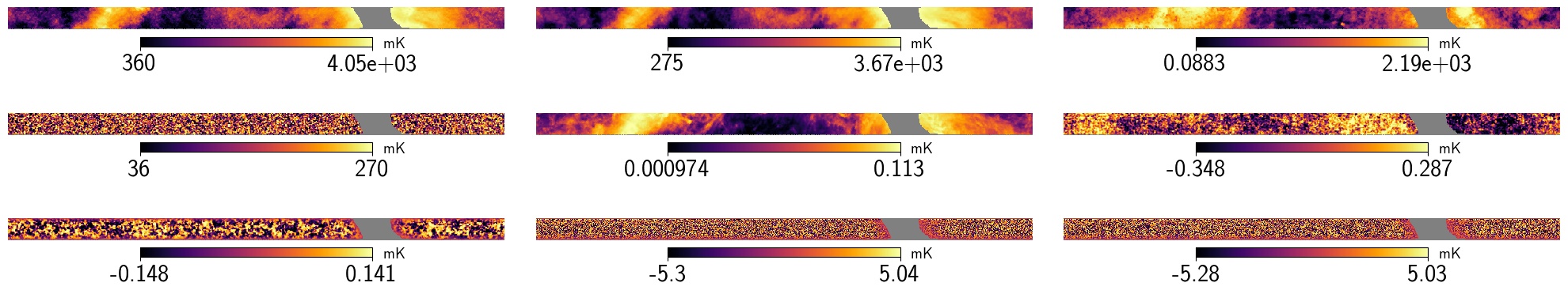
Figure 1: Intensity maps in the BINGO sky region are described in antenna temperature: observed (top left), synchrotron (top middle), free-free (top right), radio point sources (middle left), AME (center), CMB (middle right), HI (bottom left), white noise (bottom center) and, HI + white noise (bottom right). The region in gray color represents part of the Galaxy masked.

2.3 Thermal noise

Aiming to analyze the consistency and understanding of the BINGO pipeline, we assumed the instrumental noise to be thermal only. This noise was considered for a year of observing the BINGO optical design in its Phase 1 as described in (Wuensche et al., 2022).

It is crucial to keep in mind that one year of observation gives us a low level of signal stacked from the sky and, consequently, a low signal-noise ratio. BINGO expects to operate for five years, which will result in a better sensitivity than assumed in this work. But, for now, it is essential to understand how the first year and this stage of the pipeline work.

3 Modeling signals from the sky

The drift-scan IM survey cannot distinguish different signal sources from the sky and cannot specifically identify HI emissions. However, in radio astronomy, in general, there is no correlation between emissions from different parts of the sky and between different frequencies (see Fig. 2), since this occurs when the emission originates from the sum of independent systems that do not have time/phase correlations with each other (Liu & Shaw, 2020). Besides that, foregrounds have smooth spectral information, that can be modelled and used to estimate the foreground contributions. Such a process is called Foreground Removal. This process results in a signal composed of 21 cm + (instrumental) noise since their (almost) Gaussian behavior is not modelled by blind algorithms.

In summary, the estimation of 21 cm maps using a blind algorithm can be separated into two steps: (1) estimating foreground contribution to the data by exploring its spectral information; and (2) statistically estimating 21 cm maps upon adjoining noise.

The sky signals can modelled considering the contribution of the components described in sec. 2 to a sky position $p$ (here represented by a pixel with coordinates $(\phi,\theta)$, in a frequency channel $\nu_{i}$. The observed signal can be described as a linear combination of contributions from independent sources $x\left(\nu_{i},p\right)$. Assuming there are $N_{\textrm{s}}$ physical sources modelled by the blind algorithms and further signals that will not be modelled, described by $x_{21\textrm{cm}}$ and $n_{\textrm{Inst}}$, namely the 21 cm and the instrumental noise, we can thus write the observation as:

$$x\left(\nu_{i},p\right) = \sum_{j=1}^{N_{\textrm{s}}}y_{j}\left(\nu_{i},p\right)+x_{21\textrm{cm}}\left(\nu_{i},p\right)+n_{\textrm{Inst}}\left(\nu_{i},p\right)$$ (3)

$$= \sum_{j=1}^{N_{\textrm{s}}}y_{j}\left(\nu_{i},p\right)+n\left(\nu_{i},p\right),$$ (4)

where $y_{j}$ is $j$-th foreground component and $\nu_{i}$ describes the $i$-th frequency or channel. We condense 21 cm + instrumental noise into the same $n$ notation since neither is modelled by blind algorithms. We now explore the fact that the foregrounds have smooth spectral information for each sky direction $p$.

$$x\left(\nu_{i},p\right) = \sum_{j=1}^{N_{\textrm{s}}}a_{j}\left(\nu_{i},p\right)s_{j}\left(p\right)+n\left(\nu_{i},p\right)$$ (5)

$$= \sum_{j=1}^{N_{\textrm{s}}}a_{ij}\left(p\right)s_{j}\left(p\right)+n\left(\nu_{i},p\right),$$

where $a_{j}\left(p\right)$ describes the spectral law of $j$-foreground component at $p$-direction, and $s_{j}(p)$ its spatial response at $p$-direction. For different frequencies or channels, we can explore the multichannel information together and write the latter equations in a matrix formulation. If we express the different observations with the same frequency $\nu_{i}$ as $\textbf{x}\left(\nu_{i}\right)=\left[x\left(\nu_{i},p_{1}\right),\dots,x\left(\nu_{i},p_{k}\right),\dots\right]^{\textrm{T}}$, this vector covers all positions in the sky. Each such vector corresponds to a HEALPix map (Górski et al., 2005) such that we can build an $\mathbb{X}$ matrix with each row corresponding to a map produced for a different frequency, that is, $\mathbb{X}=\left[\textbf{x}\left(\nu_{0}\right),\textbf{x}\left(\nu_{1}\right),\cdots,\textbf{x}\left(\nu_{n_{\textrm{ch}}-1}\right)\right]^{\textrm{T}}$. Taking the same idea for the foreground and residual contributions, we can write

$$\mathbb{X}=\mathbb{A}\mathbb{S}+\mathbb{N},$$ (6)

where $\mathbb{S}$ is called the spatial response and $\mathbb{A}$ the mixing matrix. The former has in each row the spatial response of each foreground component and the latter has each column corresponding to a spectral law. Thus, $\mathbb{A}$, $\mathbb{S}$, and $\mathbb{X}$ ($\mathbb{N}$) have dimensions of $N_{\textrm{ch}}\times n_{\textrm{s}}$, $n_{\textrm{s}}\times N_{\textrm{pix}}$, and $N_{\textrm{ch}}\times N_{\textrm{pix}}$, respectively. We assume that $N_{\textrm{pix}}$ is the number of pixels. $N_{\textrm{s}}$ is the actual number of foreground components, which is unknown, while $n_{\textrm{s}}$ is the number of templates used to describe the total foreground emission. On the other hand with the blind algorithm we cannot know the number of sources and we take $n_{\textrm{s}}\in\left[1,N_{\textrm{ch}}\right]$. Therefore, if the algorithm for a given $n_{\textrm{s}}$ estimates $\hat{\mathbb{A}}$ and $\hat{\mathbb{S}}$, it does not exactly estimate each astrophysical component of the foregrounds, but their effectiveness in a nonphysical description of the foregrounds,

$$\hat{\mathbb{Y}}=\hat{\mathbb{A}}\hat{\mathbb{S}}$$

Estimating $\mathbb{A}$ (and $\mathbb{S}$) is a typical linear inversion problem and different methods/algorithms explore different ways to perform this task.

If the number of channels and sources is equal ($N_{\textrm{ch}}=n_{\textrm{s}}$), the mixing matrix determinant exists, and does not have any noise contribution. In that case, there is a unique solution given by exactly $\mathbb{A}^{-1}$ that provides the spatial response. However, there is a signal not modelled by the algorithm and the mixing matrix dimension is not necessarily (almost never is) equal to the number of frequency/channels. In that case, the mixing matrix has no inverse. A priori, a blind algorithm does not define neither estimates the mixing matrix dimensions. It is precisely the way of estimating the mixing matrix that characterizes each algorithm/method. One general way to solve that problem is looking for a $\mathbb{W}$ filter that, upon operating on the observational matrix, $\mathbb{X}$, gives us the estimated foreground matrix. We can understand that it downweights $\mathbb{N}$, preserving only the foreground signals

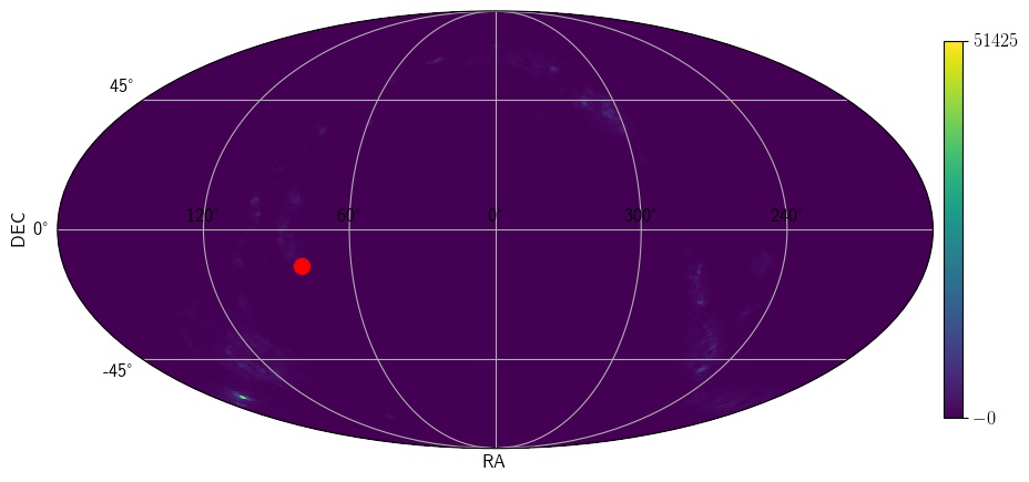
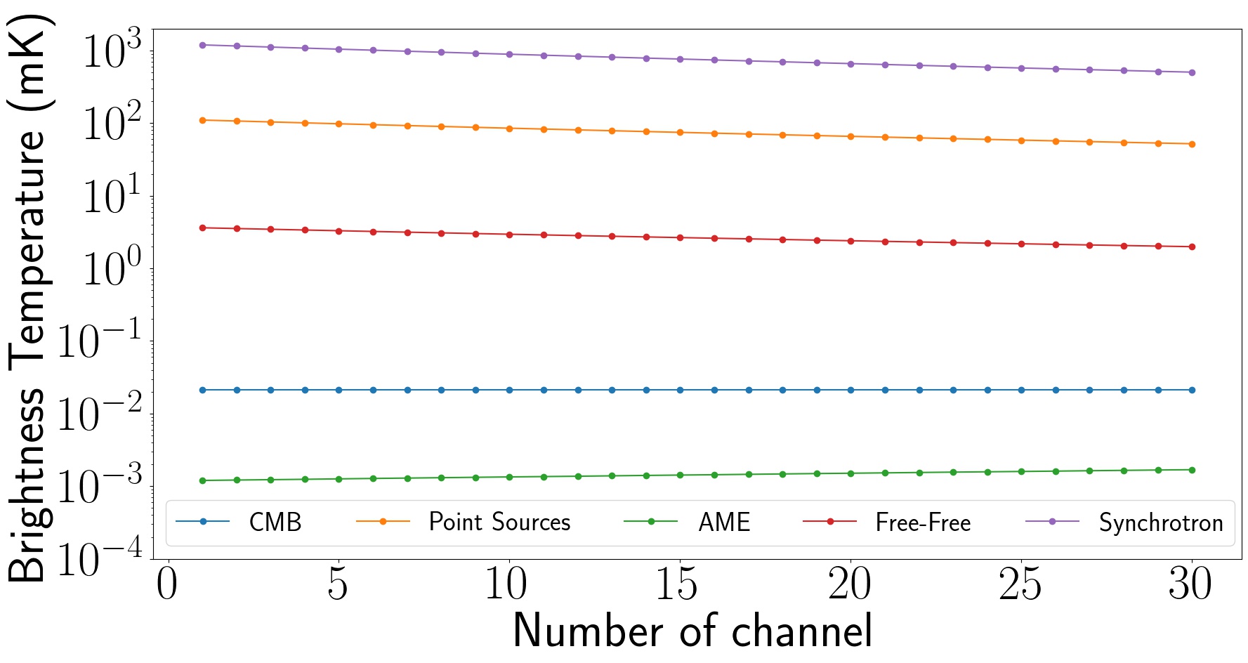
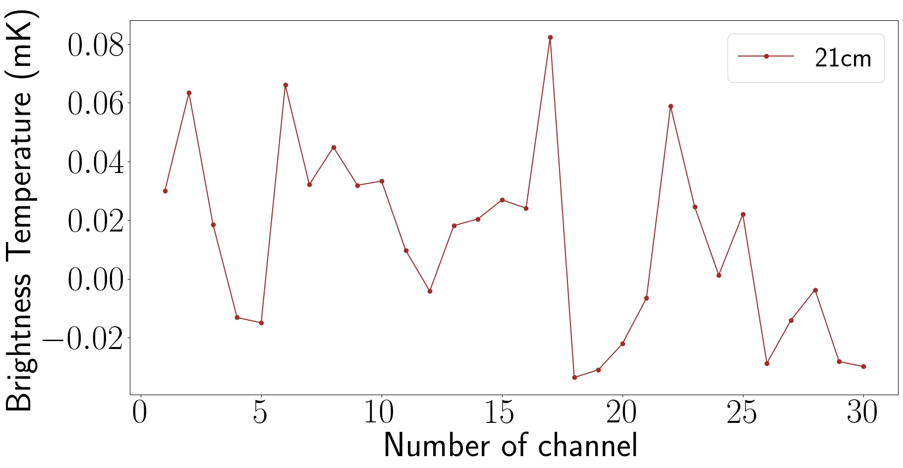
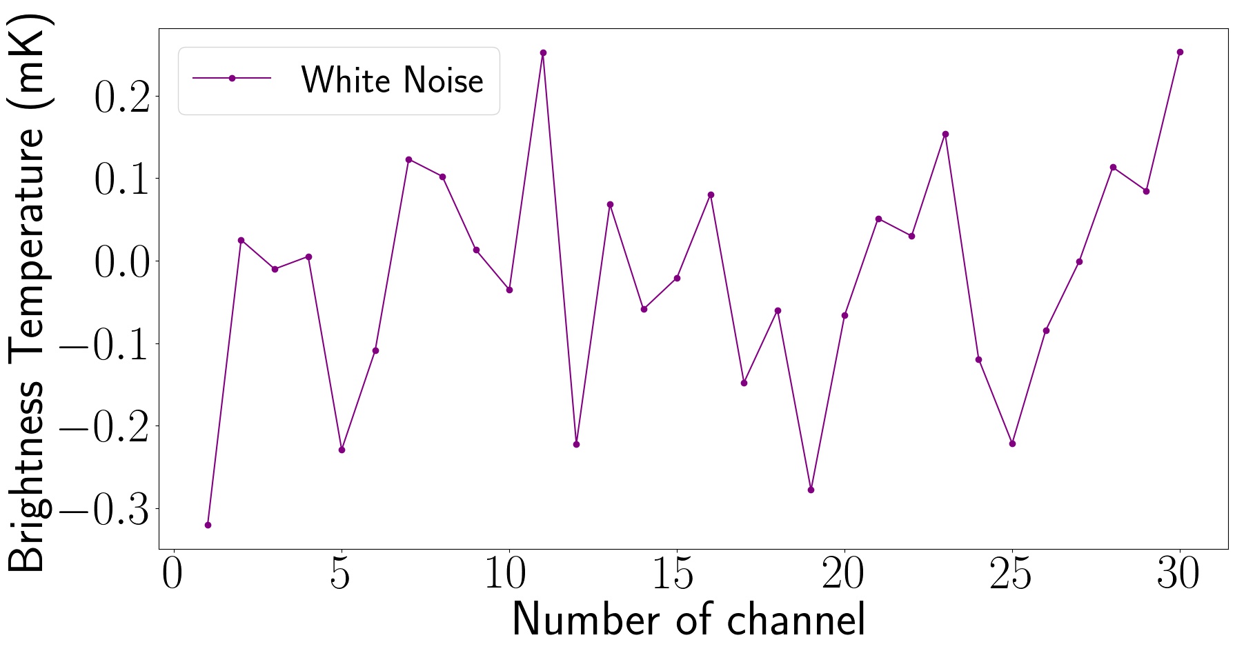
Figure 2: First image shows a red circle corresponding to (RA, DEC)=($-20.91^{\textrm{o}},12.33^{\textrm{o}}$) in celestial coordinate. In this position on the sky it is observed different emission within 960-1260 MHz. (Second row) CMB, Point Sources, AME, Free-Free and Synchrotron have smooth spectral response in that range, here divided inside 30 channels. (Third row) on the other hand, 21 cm integrated and (bottom) white noise.

$$\hat{\mathbb{S}} = \mathbb{W}\mathbb{X}$$

$$= \left(\mathbb{W}\mathbb{A}\right)\mathbb{S}+\mathbb{W}\mathbb{N}$$

Following (Hyvärinen et al., 2001), a natural way to solve that problem is trying to minimize the $\mathbb{N}$ contribution by a least-squares criterion. This is a deterministic approach to the estimation problem. No assumptions on the probability distribution are necessary,

$$\nabla_{\mathbb{S}}\bigg{|}_{\hat{\mathbb{A}},\hat{\mathbb{S}}}\left(\frac{1}{2}\|\mathbb{N}\|^{2}\right)=0,$$

that gives us

$$\mathbb{W}=\mathbb{A}^{+}=\left(\hat{\mathbb{A}}^{\textrm{T}}\hat{\mathbb{A}}\right)^{-1}\hat{\mathbb{A}}^{\textrm{T}}$$ (7)

known as Moore-Penrose pseudoinverse, $\mathbb{A}^{+}$.

We used a canonical metric with $\ell_{2}$ in the minimization, $\|\cdot\|=\|\cdot\|_{\ell_{2}}$, so far. But, we can also use another metric like e.g., $\|\cdot\|_{\textrm{Q}}$, with some $\mathbb{Q}$ matrix. In this case, the minimization is a generalization of the previous norm and is called Generalized Least Squares (GLS).

So

$$\nabla_{\mathbb{S}}\bigg{|}_{\hat{\mathbb{A}},\hat{\mathbb{S}}}\left(\frac{1}{2}\|\mathbb{N}\|_{\mathbb{Q}}^{2}\right)=0.$$

Therefore, the filter is

$$\mathbb{W}=\left(\hat{\mathbb{A}}^{\textrm{T}}\mathbb{Q}\hat{\mathbb{A}}\right)^{-1}\left(\hat{\mathbb{A}}^{\textrm{T}}\mathbb{Q}\right),$$ (8)

which also known as Gauss-Markov estimator in Information Theory.

Here, we use the definition of the difference between observational matrix and estimated matrix of foregrounds as a residual matrix given by

$$\mathbb{R}=\mathbb{X}-\hat{\mathbb{Y}}=\left(1-\mathbb{W}_{\textrm{FG}}\right)\mathbb{X},$$

where $\mathbb{W}_{\textrm{FG}}\doteq\mathbb{A}\mathbb{W}$.

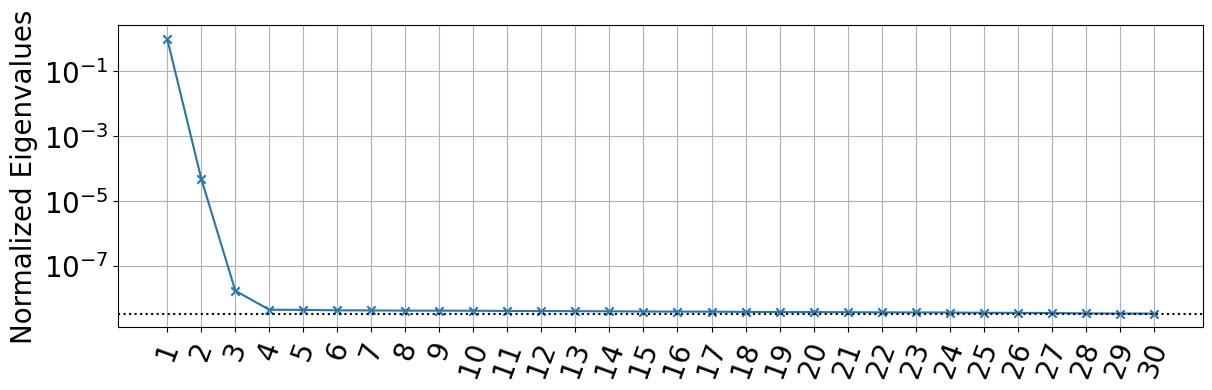
Figure 3: Normalized eigenvalues of the observational covariance matrix. Given that mixing matrix dimension is limited by number of channel, there are only three eigenvalues contributing significantly which corroborates with better results of FastICA and GMCA.

4 Foreground Removal methods

To begin with, in order to treat the sky images we must account for the undesirable foreground contribution to the total observed signal. We use here three blind methods: the algorithms do not assume any previous knowledge about the emission sources. Their general description and assumptions will be given below.

4.1 Fast Independent Component Analysis

Independent Component Analysis (ICA) is an algorithm applied to astrophysical (and cosmological) observations to model or remove foregrounds using the hypothesis that astrophysical sources are statistically (and mutually) independent. Signals from different sources being statistically independent mean that different signals do not contain information from one another. In mathematical jargon, when two signals are (statistically) independent, their joint distribution function is the product of their distributions.

ICA-based algorithms look for a linearly transformed matrix $\mathbb{\hat{S}}=\mathbb{W}\mathbb{X}$, where each row is composed of a transformed vector and all components are mutually independent (Hyvärinen, 1999). It is essential to point out here that this work uses a noise-free ICA-based algorithm. ICA-based algorithms just seek to model foregrounds, and non-smooth spectral components are leading as rest of the modelling. Let $\mathbf{w}_{i}$ be the $i$th row of $\mathbb{W}$, i.e., $\mathbb{W}=\left[\mathbf{w}_{1},\mathbf{w}_{2},\dots,\mathbf{w}_{N_{s}}\right]^{\textrm{T}}$. We can look for

$$\mathbf{y}_{i}=\sum_{j=1}^{N_{\textrm{ch}}}W_{ij}\mathbf{x}_{j}=\mathbf{w}_{i}^{\textrm{T}}\mathbb{X}$$ (9)

as an independent component, that is equivalent to look for it as a maximally non-Gaussian component (Hyvärinen et al., 2001). For each iteration, the ICA-based algorithm look for a new transformed variable that is more independent than the variable iterated previously, in the sense of minimizing the negentropy defined ahead. Thus, if we look for something like $\mathbf{y}_{i}=\mathbf{w}_{i}^{\textrm{T}}\mathbb{X}=(\mathbf{w}_{i}^{\textrm{T}}\mathbb{A})\mathbf{s}$, but for residuals, the operator $\mathbf{e}=(\mathbf{w}^{\textrm{T}}\mathbb{A})^{\textrm{T}}$ assumes the value 1 in $i$-th position of the vector, and 0 otherwise. That occurs when $\mathbf{w}_{i}$ is one of the rows of the inverse of the mixing matrix. But neither mixing matrix necessarily has an inverse nor we are dealing with a noise-free inverse problem, so we cannot know exactly what $\mathbf{w}$’s are and we need to find an estimator for them. By the central limit theorem, the linear combination $\mathbf{e}^{\textrm{T}}\mathbf{s}$ is more Gaussian than any of the components of $\mathbf{s}$ becoming least Gaussian when it is (approximately) equal to one of the components of $\mathbf{s}$, as, e.g., when $\mathbf{e}^{\textrm{T}}\mathbf{s}$ is (close to) $s_{i}$. When this happens, we get the $\mathbf{e}_{i}$ corresponding to $\mathbf{w}_{i}$.

Therefore, we need to maximize the non-Gaussianity of the $\mathbf{e}^{\textrm{T}}\mathbf{s}$ to get each component corresponding to a respective $\mathbf{e}_{i}$, or equivalently $\mathbf{w}_{i}$. That is nothing more than a search for a direction for which the components are maximally non-Gaussian. (Hyvärinen et al., 2001) suggested the negentropy function as such a measure, in contrast to the higher-order (statistical) method as kurtosis (the forth-order cumulant of a random variable) which by that ”is not a robust measure of nongaussianity”. The negentropy is defined as

$$J\left(\mathbf{\xi}\right)=H\left(\mathbf{\xi}_{\textrm{G}}\right)-H\left(\mathbf{\xi}\right),$$

where $H$ is the entropy function, $\mathbf{\xi}$ a vector, and the subscript G identifies a Gaussian random variable of the same covariance matrix as $\mathbf{\xi}$. The disadvantage of using negentropy is that it is computationally hard to calculate. So it is necessary to estimate it through some contrast function $g$,

$$J\left(\mathbf{\xi}\right)\sim\Big{[}\textrm{E}\big{\{}g\!\left(\mathbf{\xi}\right)\big{\}}-\textrm{E}\{g\!\left(\mathbf{\nu_{\textrm{G}}}\right)\}\Big{]}^{2}$$

for non-quadratic function $g$, and a Gaussian variable $\nu_{\textrm{G}}$ of zero mean and unit variance. The ICA algorithm used in this paper was the FastICA, a fast fixed-point algorithm that uses negentropy as a measure of non-Gaussianity and $\xi=\mathbf{w}^{\textrm{T}}\mathbf{z}$, where $\mathbf{z}$ is the whitened data of $\mathbf{x}$. In this work, we have used $g(\cdot)=\log\cosh(\cdot)$, with 20 maximum number of iterations and 0.01 of tolerance with FastICA by scikit-learn package to get the mix matrix and so to estimate the $\mathbb{W}$. For a complete description of the algorithm, please see (Hyvärinen et al., 2001).

4.1.1 FastICA as an optimization problem

It is straightforward to note that it is possible to describe the FastICA algorithm as an optimization problem. It aims to maximize the non-Gaussianity of the signals from negentropy we also constraint $\mathbb{W}$ matrix to be orthogonal. We define

$$\{\mathbb{W}\} = \underset{\mathbb{W}}{\textrm{argmax}}\Bigg{\{}J\left(\mathbb{W}^{\textrm{T}}\mathbb{X}\right)+\lambda\|\mathbb{W}\mathbb{W}^{\textrm{T}}-\mathbb{I}\|\Bigg{\}}$$ (10)

where argmax finds the variable $\mathbb{W}$ that maximizes the relation inside the brackets.

FastICA was introduced for the separation of astrophysical components in (Maino et al., 2002). Some works used FastICA in 21 cm cosmology in the reionization (Chapman et al., 2012) and post-reionization (Carucci et al., 2020) contexts. It is important to note that FastICA estimates neither 21 cm nor thermal noise signals: these are residuals of the process of the foreground estimation. FastICA gives a unique solution to the problem. Each column of $\mathbb{A}$ is unique up to the signal.

4.2 Generalized Morphological Component Analysis

Generalized Morphological Component Analysis (GMCA) is based on two pieces of information: morphological diversity and sparsity. We will briefly describe these properties below.

4.2.1 Sparsity and morphological diversity

A signal $\mathbf{y}$ is said to be sparse in a dictionary $\boldsymbol{\Phi}$ if it can be represented a by few elements of $\boldsymbol{\Phi}$. For instance, the signal $\mathbf{y}$ can be represented by

$$\mathbf{y}=\boldsymbol{\alpha\Phi}=\sum_{\gamma\in\Gamma}\alpha^{\gamma}\phi_{\gamma}$$

where $\alpha^{\gamma}$ is $\gamma$th coefficient of the representation. If $\mathbf{y}$ is sparse in $\boldsymbol{\Phi}$ the number of nonzero coefficients is small. More precisely, $\mathbf{y}$ is $k$-sparse in $\boldsymbol{\Phi}$ if the number of non vanishing coefficients is $k$. However, signals of practical interests, in general, are not strictly sparse. Therefore, it is important to find representations in which the signals are sparse. In this sense using wavelets for information compressing is useful since they are very well located in both spatial (or time) and frequency domains (Starck et al., 1997, 2007). Because of this feature, wavelets are useful in the sparse representation of a signal. Wavelets on the sphere are also well located in both harmonic and pixel domains, been thus of widespread use in order to analyse astrophysical maps.

The first paper to use sparsity as a source BSS problems was (Zibulevsky & Pearlmutter, 2000). The (Starck et al., 2004) shows the method of Morphological Component Analysis (MCA). It uses the sparsity idea for signals as linear instantaneous mixture from different sources through overcomplete dictionaries for representation. The method takes advantage of the sparse representation to separate features based on their morphologies. That is, sparsity and morphological diversity are extensively used. Its multichannel extension gives rise to Multichannel-MCA (MMCA), which assumes each signal source $s_{j}$ can be sparsely well represented in a given dictionary $\boldsymbol{\Phi}_{j}$. Finally, (Bobin et al., 2007) shows the GMCA, that expands MMCA to assume $s_{j}$ can be represented not only a possible dictionary, but by a linear combination of different dictionaries (here assumed as being orthogonal bases), that is, a superdictionary $\mathcal{D}=[\boldsymbol{\Phi}^{\textrm{T}}_{1},\dots,\boldsymbol{\Phi}^{\textrm{T}}_{D}]^{\textrm{T}}$. Each source $s_{j}$ has a representation given by

$$s_{j} = \sum_{k=1}^{D}\phi_{jk}=\sum_{k=1}^{D}\alpha_{j}^{\ k}\boldsymbol{\Phi}_{k},$$ (11)

or, equivalently, in a matrix representation,

$$\mathbb{S} = \boldsymbol{\alpha}\mathcal{D}.$$ (12)

We can say that $s_{j}$ is modeled as a linear combination of D-morphological components, $\{\phi_{jk}\}_{k=1}^{D}$, each being morphological component sparse in a given orthogonal base.

4.2.2 GMCA as an optimization problem

When we assume that each row (signal) of $\mathbb{S}$, is sparse in $\mathcal{D}$, we inevitably run into the problem of having more than one solution because there is more than one representation of each signal, since $\mathcal{D}$ is overcomplete. Thus we need to add some constraint to get a single solution. Indeed, since we want the most sparse representations, we seek for the representations with the least number of the coefficients. The original problem was proposed using a constraint as $\|\alpha\|_{\ell_{0}}$ that is a $\ell_{0}$-regularization problem, but this one is not computationally efficient, since it is a non-convex and combinatorial problem. We can ou problem from a an ${\ell_{0}}$ to a $\ell_{1}$-regularization problem using $\|\alpha\|_{\ell_{1}}$,

$$\{\hat{\mathbb{A}},\boldsymbol{\hat{\alpha}}\} = \underset{\mathbb{A},\boldsymbol{\alpha}}{\textrm{argmin}}\Bigg{\{}\|\mathbb{X}-\mathbb{A}\boldsymbol{\alpha}\mathcal{D}\|^{2}_{\textrm{F},\mathbb{C}^{-1}_{\mathbb{N}}}+2\lambda\sum_{j=1}^{N_{s}}\|\alpha_{\!j}\|_{\ell_{1}}\Bigg{\}}$$ (13)

with the norm of the first term being the Frobenius norm with respect to inverse of the noise covariance matrix, $\mathbb{C}_{\mathbb{N}}$, and $\lambda$ is a regularization parameter important to the thresholds. We do not detail the algorithm, which can be seen in (Bobin et al., 2007, 2006); we can resume the algorithm idea, in each $i$th iteration, by starting with $\mathbb{A}^{(i-1)}$ to estimate $\mathbb{S}^{(i)}$, and then update the mix matrix to new estimation, $\mathbb{A}^{(i)}$. Which can be done first by applying hard-thresholding operator in $\mathbb{S}^{(i-1)}$ description estimate in $\mathcal{D}$, and latter backward transform to real domain: $\mathbb{S}^{(i)}=\textrm{HT}_{\lambda^{(i-1)}}\!\left[\mathbb{A}^{(i-1)+}\mathbb{X}\mathcal{D}^{\textrm{T}}\right]\mathcal{D},$ where $\lambda^{(i-1)}$ is the $i$th threshold. Thereafter, we need to update the mix matrix $\mathbb{A}^{(i)}=\mathbb{X}\mathbb{S}^{(i)+}$.

In this work, we used starlet as a dictionary (Starck et al., 2007), that is a well known spherical wavelet transform in astronomical image analysis, since it explores the features from astrophysical objects that are more or less isotropic (in most cases). We used a starlet decomposition with a scale of decomposition as can be seen in the Fig. 4, where there is a map with 21cm + foregrounds (first row), its scale coefficient map (second row) and wavelet coefficient map (third row).

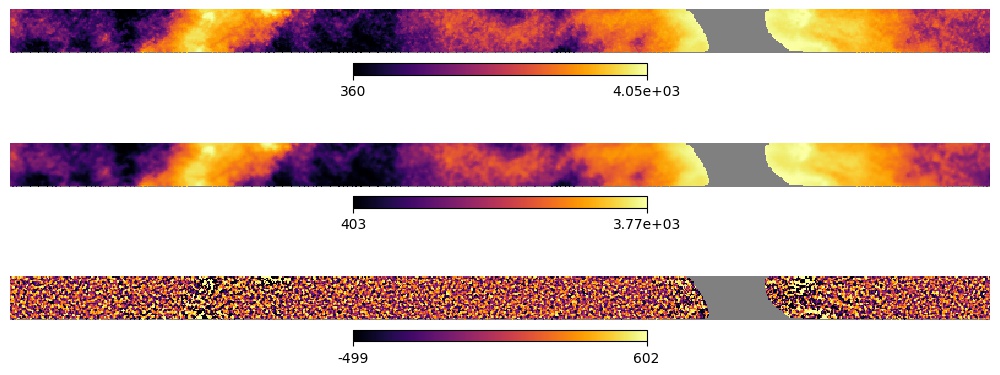
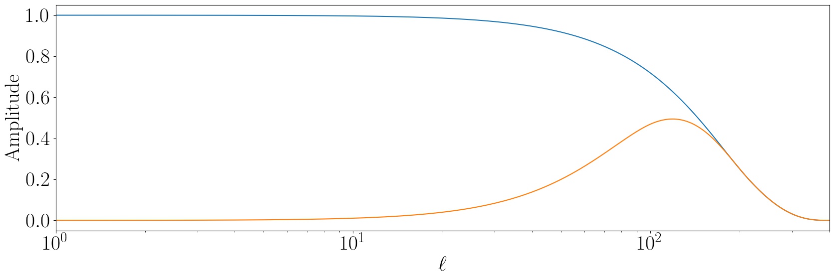
Figure 4: The first row is the input map composed of all foregrounds and 21 cm emission. The input map transformed by starlet transformation can be seen in the second and third rows, where we have a starlet coarse coefficient and the starlet detail coefficient maps, respectively. The last row represents (blue) spherical scaling function and (orange) spherical wavelet function at the null scales.

4.3 Generalized Needlet Internal Linear Combination

As the effective ratio between 21 cm and observational signals depends on the pixels (i.e., direction), the number of the (nonphysical) templates to describe the contribution of the foregrounds changes across the sky. This fact can be checked if we look at the ratio in the directions of the Galaxy and outside of Galaxy. Also, although thermal noise and 21 cm signals follow a Gaussian distribution among channels, foregrounds do not, and that ratio depends on the spectrum too. Then, it is essential to have a detailed description of the foregrounds contribution to both spatial and spectral information. Moving the spectral analysis to the harmonic domain, we can use the localized filtering needlets feature (Marinucci et al., 2008). In the Fig. 5, we can see the specific needlets described in (Basak & Delabrouille, 2013) through a set of cosine filters with bandcenters 0, 128 and 383, each corresponding to a finite number of the multipoles (needlet bands). Each needlet band decomposes the observational map in different scales, as shown in Fig. 5.

Delabrouille et al. (2009) applied the Internal Linear Combination (ILC) in the needlet space for the WMAP data, called it Needlet-ILC (NILC) to extract the CMB maps. Remazeilles et al. (2011) generalized it as a multidimensional filter in a new algorithm called Generalized-NILC (GNILC). He modelled the observation as multidimensional components (templates) instead of one single template.

4.3.1 GNILC as an optimization problem

Roughly speaking, GNILC algorithm can be resumed as a search for a filter that has a unitary response for the target signal and blocks the others. Following (Remazeilles et al., 2011) we can described it as an optimization problem,

$$\{\hat{\mathbb{A}},\hat{\mathbb{S}}\}=\underset{\mathbb{A},\mathbb{S}}{\textrm{argmin}}\Bigg{\{}\|\mathbb{W}\|^{2}_{\textrm{F},\mathbb{R}^{-1}_{\mathbb{X}}}+\|\Lambda^{\textrm{T}}\left(\mathbb{A}-\mathbb{W}\mathbb{A}\right)\|_{\textrm{F}}\Bigg{\}},$$ (14)

where $\Lambda$ is a matrix containing Lagrange multipliers. The solution of this problem is exactly Eq. 8 with $\mathbb{Q}=\mathbb{R}^{-1}_{\mathbb{X}}$. However, GNILC does that in needlet space; that is, using the covariance matrix of the needlet coefficients in each range of multipoles, obtaining a filter per needlet bands, and then estimating foregrounds contribution in those. Finally, applying inverse needlet transform in these last maps to estimate the foreground maps in real space.

GNILC uses a prior angular power spectrum of the target signal to measure the signal-noise ratio and separate the degree of freedom of the target and unwanted signals. That is, it uses the prior template of the 21-cm signal to measure the degrees of freedom of the foreground contribution, $N_{s}$, in the observation per needlet bands and pixel.

For 21 cm maps, GNILC was first used by Olivari et al. (2016). Unlike the previous GNILC works, Olivari et al. (2016) uses $N_{s}$ to represent degrees of freedom of foregrounds + instrumental noise, and estimates its value using the Akaike Information Criterium (AIC) method (Akaike, 1974; Bozdogan, 1987). Here, we separate the foregrounds from the 21 cm and (instrumental) noise. They are projected onto a $(n_{\textrm{ch}}-N_{s})$-dimensional subspace. In other words, GNILC operates a singular value decomposition (SVD) of the whitened data covariance matrix,

$$\mathbb{\hat{R}}^{-1/2}_{\textrm{prior}}\mathbb{R_{\mathbb{X}}}\mathbb{\hat{R}}^{-1/2}_{\textrm{prior}}=\mathbb{\hat{U}}\mathbb{\hat{D}}\mathbb{\hat{U}}^{\dagger},$$ (15)

where $\mathbb{\hat{R}}_{\textrm{prior}}$ is the covariance matrix of the prior template, and $\mathbb{\hat{U}}$ and $\mathbb{\hat{D}}$ are matrices composed of eigenvectors and eigenvalues of the term on the left hand in Eq. 15, respectively. The matrix of the eigenvectors is split into a part of foregrounds (FG) contribution and another part of 21cm + noise (21cm+N), $\mathbb{\hat{U}}=\left[\mathbb{\hat{U}}_{\textrm{FG}},\mathbb{\hat{U}}_{21\textrm{cm}+\textrm{N}}\right]$. The AIC estimates the dimension of the 21cm + noise space, that is, the dimension of $\mathbb{\hat{U}}_{21\textrm{cm}+\textrm{N}}$. Thus, GNILC obtains the mixing matrix by

$$\mathbb{\hat{A}}=\mathbb{\hat{R}}_{\textrm{prior}}^{1/2}\mathbb{\hat{U}}_{21\textrm{cm}+\textrm{N}},$$ (16)

With the mixing matrix estimated and the needlet coefficient covariance matrix, GNILC estimates the multidimensional ILC filter in each pixel and bandwidth, identified here by $j$,

$$\hat{\mathbf{x}}^{(j)}_{21\textrm{cm}+N}(p)=\mathbb{W}^{(j)}(p)\mathbf{y}^{(j)}(p).$$ (17)

with $\hat{\mathbf{x}}^{(j)}_{21\textrm{cm}+N}(p)$ the multichannel 21cm + noise estimation per pixel and in $j$th bandwidth. After doing all the needlet bands and estimating all the target signal per pixels and range of multipoles, GNILC performs the inverse needlet transform (INT) and gives the 21cm+noise maps in the pixel space,

$$\{\hat{\mathbf{x}}^{(j)}_{21\textrm{cm}+N}(p)\}\stackrel{{\scriptstyle\textrm{INT}}}{{\longrightarrow}}\hat{\mathbf{x}}_{21\textrm{cm}+N}(p)$$

For a complete description of the algorithm, please see (Fornazier et al., 2022). As a prior, we used a template for each channel of an arbitrary realization of 21cm + white noise.

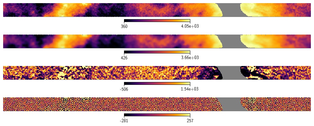
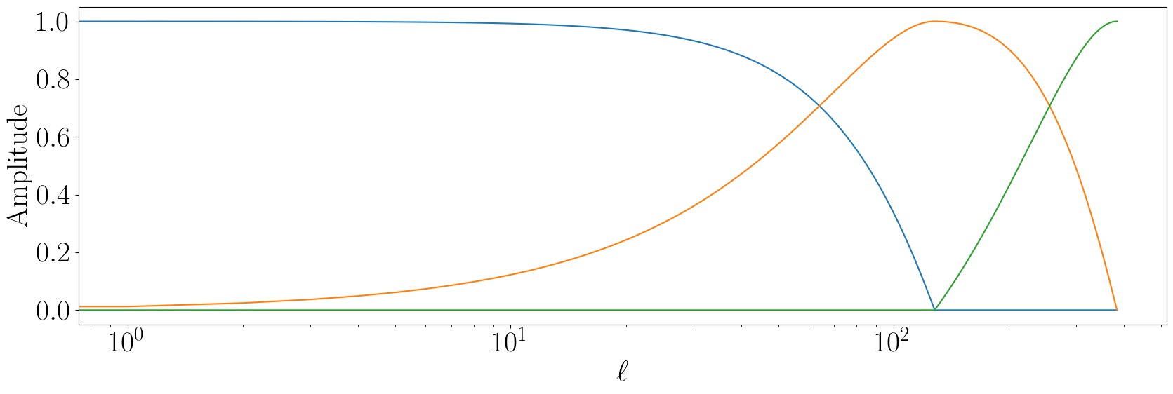
Figure 5: The first row is the input map composed of all foregrounds and 21 cm emission. The input map transformed by needlet transformation can be seen in the three next images. The second row is the needlet coefficient map from null bandcenter, the third for bandcenter 128, and the forth for 383. The last plot represents (blue) spherical scaling function and (orange) spherical wavelet function.

4.4 General Observations

It is worth stressing that we first used all maps in all channels using HEALPix NSIDE=512 resolution, convoluted with a main Gaussian beam with FWHM=40 arcmin Then the convoluted maps are degraded to NSIDE=256. This is an idealistic assumption since not all feed horn beams have the exact Gaussian shape. Indeed, although the central feed horn in the focal plane has a very Gaussian main beam, the farther the feed horn is from the center of the focal plane, the less Gaussian its main beam will be. Furthermore, the way reflectors are constructed also significantly alter the main beam of the feed horns. The BINGO reflectors will be built modularly, connecting $\sim$ 1x2 m² panels. This construction affects the beam shape, mainly the more distant lobes. (Abdalla et al., 2022b) describes the BINGO optical design. The description of the effects of building the reflectors will be described in a future paper.

The main beams can also depend on the frequency. These different effects lead to a more complex foreground removal process, and the algorithms need to be adapted to that situation. We shall deal with these issues in future works.

5 Noise debias process

After subtracting the foreground contributions to the ”observed” maps, we need to estimate the 21 cm signal, extracting it from a residual map composed of 21-cm signal and instrumental noise.

$$\hat{\mathbb{X}}_{\textrm{FG}}\doteq\hat{\mathbb{Y}}=\mathbb{W}_{\textrm{FG}}\mathbb{X}.$$

Therefore,

$$\hat{\mathbb{X}}_{21\textrm{cm}+\textrm{N}}=\mathbb{X}-\mathbb{W}_{\textrm{FG}}\mathbb{X}.$$

We used between 25 and 400 different simulated 21 cm and noise maps. Estimating 21 cm power spectrum is done here using ANAFAST, an angular power spectrum estimator from HEALPix. Let $a^{\textrm{(F)}}_{\ell,m}$ be the harmonic coefficients for a F field. The angular power spectrum for F is given by $C_{\ell}^{\textrm{(F)}}=(2\ell+1)^{-1}\sum_{m=-\ell}^{\ell}a_{\ell m}^{\textrm{(F)}\dagger}a^{\textrm{(F)}}_{\ell m}$.

From now on we rely on the notation ${}_{\left(\textrm{b}\right)}^{\left(a\right)}\hat{C}^{\left(c\right)}_{\ell}$ where $a$, $b$ and $c$ denote realization, algorithm used to estimate the foreground contribution (GNILC, GMCA or FastICA) and type of map (for instance, 21 cm and/or noise N), respectively. The ”hat” $\hat{}$ defines the estimated value of the angular power spectrum derived from the debiasing process. Therefore, for a specific $M$ algorithm and a specific $L_{i}$ realization, the estimated 21 cm angular power spectrum is:

$${}_{\left(\textrm{M}\right)}^{\left(L_{i}\right)}\hat{C}^{\left(21cm\right)}_{\ell} = \frac{{}_{\left(\textrm{M}\right)}^{\left(L_{i}\right)}C^{\left(\textrm{R}\right)}_{\ell}}{S_{\ell}}-\bigg{\langle}{}^{\left(L_{j}\right)}C^{\left(\textrm{N}\right)}_{\ell}\bigg{\rangle}_{L_{j}}^{j\neq i},$$

where R is the residual, that is, the components not modeled by the algorithm (21 cm and N) plus foregrounds modeling error; and

$$S_{\ell} = \Bigg{\langle}\frac{{}_{\left(\textrm{M}\right)}^{\left(L_{j}\right)}C^{\left(\textrm{R}\right)}_{\ell}}{{}^{\left(L_{j}\right)}C^{(\textrm{21cm + N})}_{\ell}}\Bigg{\rangle}_{L_{j}}^{j\neq i},$$ (18)

and $\langle\rangle_{L_{j}}^{j\neq i}$ describes the average over all realizations except the $L_{i}$ realization; that is, for $L_{j}\in\left(L_{0},\cdots,L_{i-1},L_{i+1},\cdots,L_{n_{r}-1}\right)$.

6 Statistical tools

We used a resampling method to estimate the variance of each angular power spectrum recovered after foreground removal and noise debiasing. We tested both Jackknife and Bootstrap methods and did not identify any relevant distinction between them. So we decided to use Jackknife because it is computationally faster. We applied $\chi^{2}$ per multipole tests to assess the statistical quality of the results.

6.1 Jackknife variance estimator

The Jackknife method is a resampling strategy that works by sequentially deleting one observation at a time in a given data set, then recomputing the desired statistics. In our case, we want to estimate the variance of the angular power spectrum for each multipole and channel. We thus define a vector containing the angular power spectrum with fixed multipole $\ell$ and channel $\nu$ and all, except the specific $i$-th, $N$ different realizations.

$${}^{\left(-i\right)}\textbf{C}_{\ell}\doteq\left({}^{\left(L_{0}\right)}C_{\ell},\cdots,{}^{\left(L_{i-1}\right)}C_{\ell},{}^{\left(L_{i+1}\right)}C_{\ell},\cdots,{}^{\left(L_{n_{r}-1}\right)}C_{\ell}\right)^{\textrm{T}}.$$

Thus, we can build $n_{r}$ new samples from the original one. Let $G$ be a function that gives some estimator associated with the sample. We can define the estimators by

$${}^{(-i)}\hat{\theta}_{(\ell)} = G\left({}^{\left(-i\right)}\textbf{C}_{\ell}\right).$$

It is convenient to define a matrix composed of all estimator values

$${}^{(-i)}\hat{\Theta}=\left({}^{(-i)}\hat{\theta}_{(\ell_{\textrm{min}})},\ \cdots,{}^{(-i)}\hat{\theta}_{(\ell_{\textrm{max}})}\right)^{\textrm{T}}$$

Assuming $G$ to be the function that calculates the mean value,

$${}^{(-i)}\hat{\theta}_{(\ell)}=\frac{1}{n_{r}}\sum_{\underset{j\neq i}{j=0}}^{n_{r}-1}{}^{\left(L_{j}\right)}C_{\ell},$$ (19)

we can get the Jackknife variance by

$$\hat{\sigma}=\frac{n_{r}-1}{n_{r}}\sum_{j=0}^{n_{r}-1}\left({}^{(-j)}\hat{\Theta}-\langle\Theta\rangle\right)\left({}^{(-j)}\hat{\Theta}-\langle\Theta\rangle\right)^{\textrm{T}},$$ (20)

where

$$\langle\Theta\rangle:=\frac{1}{n_{r}}\sum_{j=0}^{n_{r}-1}{}^{(-j)}\hat{\Theta}.$$

6.2 The $\chi^{2}$ test

To quantify our results, we have used the $\chi^{2}$ test, which is a measure of the goodness-of-fit of the model to the estimated data. We also used the Jackknife variance described in sec. 6.1 (Eq. 20) as an estimator of the variance for each angular power spectrum per multipole and per channel.

Considering the vector of the angular power spectrum of a $X$ map ($X$ is arbitrary here) on a specific channel $\nu$ as being $\textbf{C}^{X}\left(\nu\right)=\left(C^{X}_{\ell_{\textrm{min}}}\left(\nu\right),C^{X}_{\ell_{\textrm{min}}+1}\left(\nu\right),\cdots,C^{X}_{\ell_{\textrm{max}}}\left(\nu\right)\right)$, we can calculate the $\chi^{2}$ for a specific $i$-realization, $L_{i}$, and $M$-algorithm, i.e., $M\in\{\textrm{GNILC},\ \textrm{GMCA},\ \textrm{FastICA}\}$, as

$${}_{\left(M\right)}^{\left(L_{i}\right)}\chi^{2}\left(\nu,\ell\right)=\frac{\left({}^{(L_{i})}_{(M)}\hat{C}_{\ell}^{21cm}\left(\nu\right)-{}^{(L_{i})}C_{\ell}^{\textrm{input}}\left(\nu\right)\right)^{2}}{\hat{\sigma}_{\ell}^{2}\left(\nu\right)}$$ (21)

with $\hat{\sigma}^{2}\left(\nu\right)=\left(\hat{\sigma}^{2}_{\ell_{\textrm{min}}}\left(\nu\right),\cdots,\hat{\sigma}^{2}_{\ell_{\textrm{max}}}\left(\nu\right)\right)$ vector calculated by Jackknife resampling method.

Other interesting measures are those which can quantify a similar $\chi^{2}$ quantity per channel and a general $\chi^{2}$, considering all contributions in multipoles and channels. The former can be defined as the average of all $\chi^{2}$ in the same channel summing over all multipoles between a minimum and maximum values, $\ell_{\textrm{min}}$ and $\ell_{\textrm{max}}$, respectively, and dividing by its dimension,

$${}_{\left(M\right)}^{\left(L_{i}\right)}\chi^{2}_{\textrm{eff}}\left(\nu\right)=\frac{1}{n_{\ell}}\sum_{\ell=\ell_{\textrm{min}}}^{\ell_{\textrm{max}}}{}_{\left(M\right)}^{\left(L_{i}\right)}\chi^{2}\left(\nu,\ell\right),$$ (22)

where $n_{\ell}$ is the length of $\ell=\left(\ell_{\textrm{min}},...,\ell_{\textrm{max}}\right)$. The general $\chi^{2}$ is the average of the values of both channels and multipoles,

$${}_{\left(M\right)}^{\left(L_{i}\right)}\chi^{2}_{\textrm{overall}}=\frac{1}{n_{\nu}}\sum_{\nu=0}^{n_{\nu}-1}{}_{\left(M\right)}^{\left(L_{i}\right)}\chi^{2}_{\textrm{eff}}\left(\nu\right).$$ (23)

Another measurement which we used, similar to the 22, is the mean over channels

$${}_{\left(M\right)}^{\left(L_{i}\right)}\chi^{2}_{\ell}=\frac{1}{n_{\nu}}\sum_{\nu=0}^{n_{\nu}-1}{}_{\left(M\right)}^{\left(L_{i}\right)}\chi^{2}\left(\nu,\ell\right),$$ (24)

7 Results

7.1 Influence of mixing matrix dimension on the GMCA and FastICA estimations

The choice of sky masking, on top of the fixed BINGO survey area, is an important decision which impacts the recovery of the signal and reduces the contamination by different foregrounds. Fig. 6 shows the angular power spectrum of the foreground components chosen for this analysis. Dashed lines correspond to a power spectrum of the full sky and full lines correspond to a partial sky (BINGO survey area with the region around the Galactic plane also removed). The ”unmasked” power spectrum show three components (synchrotron, free-free and FRPS) with significantly more power than the other two (AME and CMB). They overlap each other and the contributions of FRPS and free-free switch positions after masking the sky to recompute the power spectrum. Synchrotron emission clearly dominates the sky in both cases, and masking the sky increases the contribution of FRPS, reducing its difference from the free-free emission, with both contributing almost equally to the total power at $l\leq 10$.

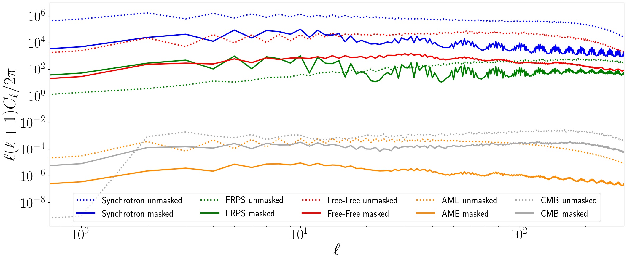
Figure 6: Angular power spectrum masked (solid line) and unmasked (dashed line) within BINGO coverage region for all foreground components assumed in this work: CMB (gray), AME (orange), Free-Free (red), FRPS (green), and Synchrotron (blue).

In contrast to the GNILC algorithm, FastICA and GMCA do not have a native way to measure the foreground contribution on the observation maps, i.e., they do not estimate $N_{s}$. Please note that $N_{s}$ is the number of foreground components of the simulated sky, as described in sec. 4.3.1, and $n_{s}$ is the number of non-physical templates assumed to represent the total foreground signals. As in the context of blind foreground removal, it is not known a priori which foreground components make up the observations. Therefore, it is necessary to have a way to choose $n_{s}$. GNILC uses AIC method per needlet band and per pixel. For the GMCA and FastICA, we computed the normalized eigenvalues from the observational covariance matrix, as shown in Fig. 3. The 21 cm + instrumental noise are subdominant in the observation data, since foregrounds are stronger than their brightness temperature by up to six orders of magnitude. As a consequence, the eigenvalues are almost all dominated by the foregrounds. Then, we can see three or four eigenvalues corresponding to almost all information contained in the observations. However, this choice has a subtle issue because the $n_{s}$ value may be larger or smaller than needed. If the $n_{s}$ is larger, the foreground removal process can be so aggressive as to extract also the 21 cm signal. If the value is smaller, the foreground removal process would still keep some foreground signal in the data, contaminating the 21 cm + instrumental noise information. It is expected that the impact of such a choice affects the final results even after noise debiasing and an analysis using different $n_{s}$ is performed.

We used three configurations for FastICA and GMCA, $n_{s}\in\{2,3,4\}$. All FastICA analysis was done with 400 realizations and in pixel space. The quality of the results was expressed as $\chi^{2}_{\textrm{eff}}$, corresponding to $\chi^{2}$ per channel, in Fig. 7. The variance was estimated by Jackknife, taking different realizations as the reference in the noise debiasing process and generating $\chi^{2}_{\textrm{eff}}$ for each configuration. But we used the same realization for each $n_{s}$ plots in Fig. 7. The black dashed line represents $\chi^{2}_{\textrm{eff}}=1$. For $n_{s}=2$, although $\chi^{2}_{\textrm{eff}}$ of the FastICA configuration is compatible with 1 for all channels, its variance is large enough to be compatible with values larger than 1. Only two non-physical templates to describe the foreground influence lead to an amount of foreground information leakage to 21 cm + instrumental noise, and then the 21 cm angular power spectrum estimated will be larger.

On the other hand, if we take $n_{s}=4$, the variances of the $\chi^{2}_{\textrm{eff}}$ are almost all smaller than $n_{s}=2$ case and all values are compatible at one sigma level with $\chi^{2}_{\textrm{eff}}=1$. Even for $n_{s}=4$, the variance values are large, and the third channel is representative of the amplitude of the variance because there are more fluctuations between the realizations assumed and, most likely that those amplitude is due to the more aggressive estimation of the foregrounds, leading to a loss of 21 cm signal. As this addition has a minor eigenvalue, just a subtle change occurs. The red line describes the best results with small variances and almost all values compatible with one, as shown in the below representation in Fig. 7.

Figure 7: Effective chi-square - that is, chi-square over multipoles per channel - for three different numbers of mixing matrix dimensions through FastICA algorithm: 2 (black), 3 (red), and 4 (blue). The plot below is an enlargement of the plot above in order to focus on red solid line behavior. The error bars were obtained from the Jackknife method over 400 realizations.

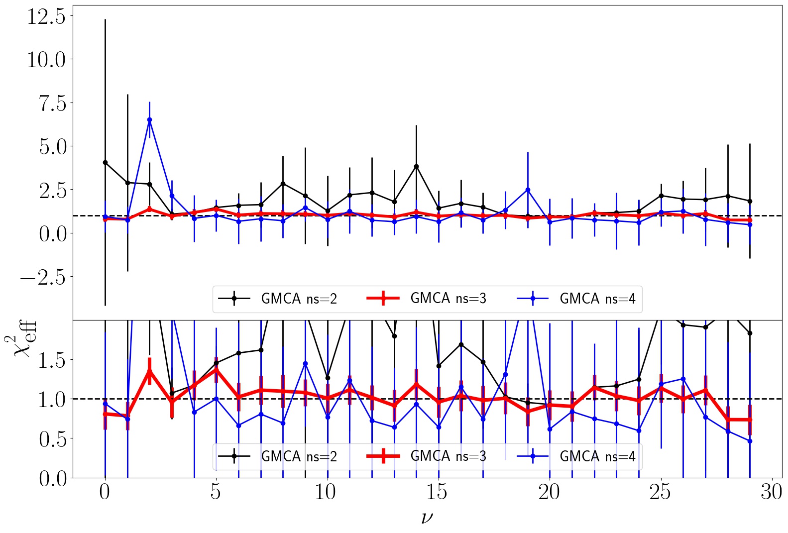
Figure 8: Effective chi-square - that is, chi-square over multipoles per channel - for three different numbers of mixing matrix dimensions through GMCA algorithm: 2 (black), 3 (red), and 4 (blue). The plot below is an enlargement of the plot above in order to focus on red solid line behavior. The error bars were obtained from the Jackknife method over 400 realizations.

The explanation for $n_{s}=3$ being the best choice is because synchrotron, free-free, and FRPS emissions are the dominant components of emission in the declination range between -24^o and -8^o in celestial coordinates. There is a strong influence not only by synchrotron and free-free but by FRPS too. FRPS importance is shown in Fig. 9, where we have a measurement of the total variance of the temperature fields given by

$$\langle\Delta^{2}\rangle(\ell_{max})=\int_{2}^{\ell_{max}}d\ln\ell\ \frac{\ell(\ell+1)}{2\pi}C_{\ell},$$ (25)

where $\ell_{max}\in\{2,3,...,300\}$. Basically, the integrated term above is the variance per $\ln\ell$, and the area below that term is the total variance. That figure is for our tenth channel. It is possible to see three principle foreground components in our sky region, which explains why we need three non-physical templates to describe the foreground contribution to the observational data.

Fig. 9 shows that the total variance of the 21cm signal (+ noise) exceeds the total AME variance when integrating multipoles up to an $\ell_{max}>20$ and the total CMB variance when integrating multipoles up to an $\ell_{max}>300$. That is crucial information because that range is where happen better estimation of the 21 cm angular power spectrum. Below that range, there is a higher variance of the angular power spectrum estimated, and above one, the estimation is worst with a smaller variance, as shown in Fig. 10. $\chi^{2}_{\ell}$ is similar to Eq. 22 but over channels and not multipoles, as described in Eq. 24.

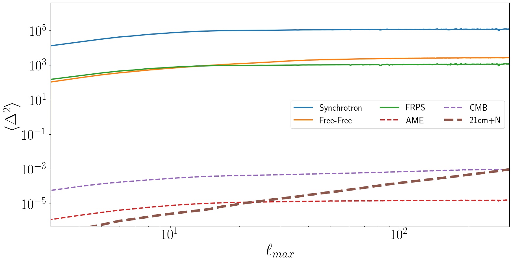
Figure 9: The total variance of the temperature field (Eq. 25) of each foreground component and of the components that are not modeled by the algorithms. Correspond to the foreground synchrotron (blue), Free-Free (orange), FRPS (green), AME (red), and CMB (violet). The total variance of the sum of 21cm signal and white noise is shown in dashed brown. Solid lines represent the component with higher contributions to the signal and the dashed one the lower contributions.

Similar results were obtained with GMCA but in sparse decomposition in the starlet transform. The results for GMCA are shown in Fig. 8, and the $\chi^{2}_{\textrm{overall}}$ values are showed in Table 1. In the table, it is possible to see that FastICA and GMCA are statistically equal when no other parameters are changed.

$n_{s}$	FastICA	GMCA
2	1.8(4)	1.8(4)
3	1.02(4)	1.02(4)
4	1.1(2)	1.1(2)

Table 1: $\chi^{2}_{\textrm{overall}}$ for different number of mixing matrix dimension assuming 400 realizations.

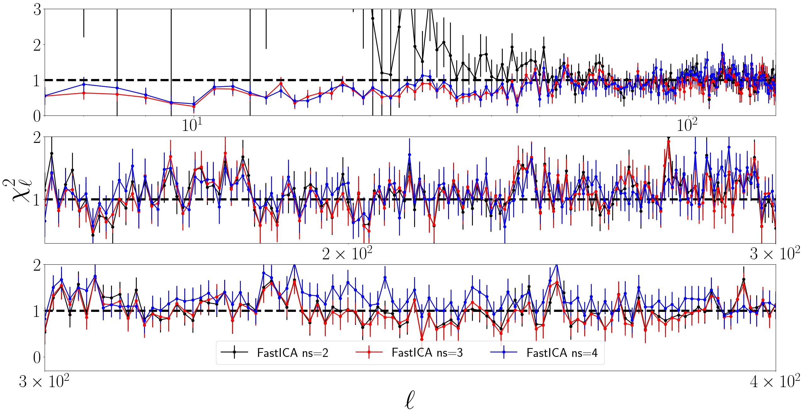
Figure 10: $\chi^{2}_{\ell}$ is the $\chi^{2}(\nu,\ell)$ mean over the channels. There are three different plots - displayed in three windows- each one with a certain number of non-physical templates (ns) to reconstruct the foreground contribution with FastICA and then debias the residuals for 400 realizations. Each window (row) represents a range of the multipole: 0-20, 21-300, and 301-400. The region within 20-300 corresponds to the better results for reconstruction; at the same time, it is the region where the 21cm + white noise (prior) is higher than AME and smaller than CMB emissions.

7.2 Influence of the number of realizations on the estimations

Employing FastICA and GMCA with $n_{s}=3$, but changing the number of simulations, we would inquired about the dependence of which algorithm of $N_{r}$. It is essential because in this period when BINGO pipelines are been built it is necessary to run 21 cm estimation several times. But to know how many simulations are sufficient to get an accurate estimate makes analysis processes faster.

In Fig. 11, we see $\chi^{2}_{\textrm{eff}}$ for five different numbers of simulations for the three methods. Regarding FastICA and GMCA values, it is possible to verify that only for 400 realizations both algorithms have a statistically similar shape. FastICA seems to converge faster to the shape of the $\chi^{2}_{\textrm{eff}}$ with 400 realizations than GMCA. The results become clearer in Table 3, where it is shown that only 25 realizations for all results of the algorithms are not compatible with one. All other numbers are statistically compatible. GMCA and FastICA only have the same shape with 400 realizations and $n_{s}=3$. It seems for a higher number of realizations on the estimation, in our configuration, both algorithms converge to the same shape and as the same $\chi_{\textrm{overall}}^{2}$.

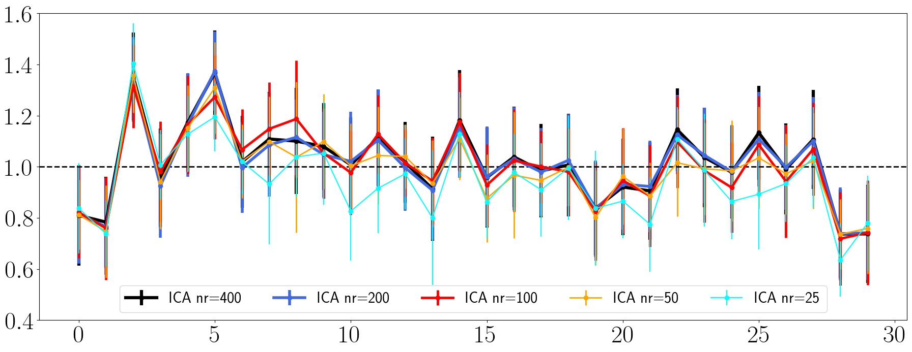
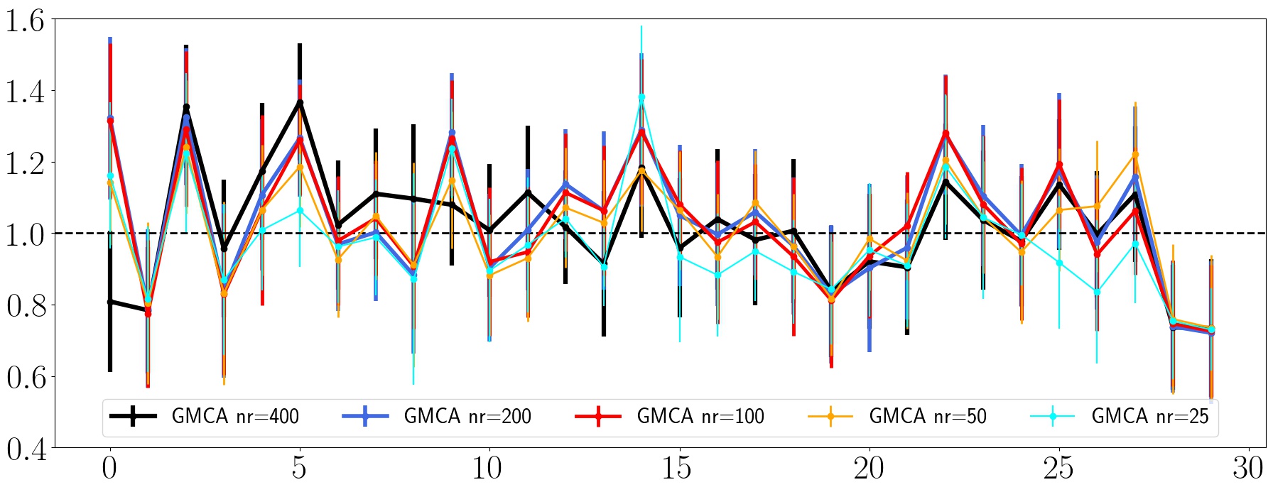
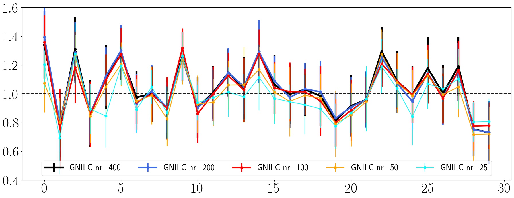
Figure 11: Effective $\chi^{2}$ per channel for FastICA (top left), GMCA (top right), and GNILC (bottom) for five number of simulations used: 25 (cyan), 50 (orange), 100 (red), 200 (blue), and 400 (black).

$n_{r}$	GMCA	FastICA	GNILC
400	1.02(4)	1.02(4)	1.04(4)
200	1.04(4)	1.01(4)	1.04(4)
100	1.03(3)	1.01(4)	1.03(3)
50	1.01(3)	0.99(3)	1.01(3)
25	0.97(4)	0.95(3)	0.97(4)

Table 2: $\chi^{2}_{\textrm{overall}}$ for different numbers of simulations assuming GMCA and FastICA with dimension

7.3 Comparison between GNILC, GMCA and FastICA algorithms

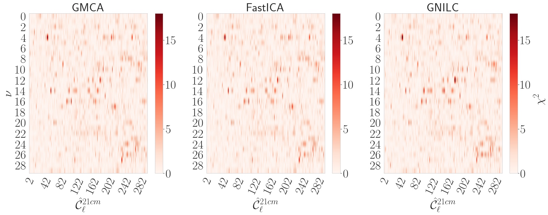
Figure 12: The plots are the $\chi^{2}$ (Eq. 21) heat map of the three algorithms. The vertical axis corresponds to the channel, and the horizontal one to the reconstructed HI angular power spectrum corresponding to a specific multipole. The redder values concerning HI angular power spectrum are harder to estimate.

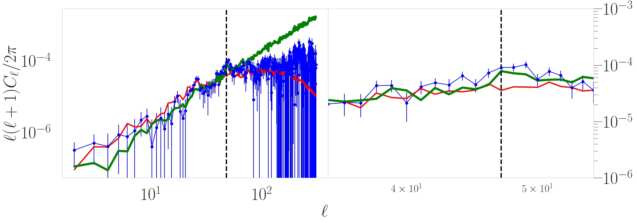
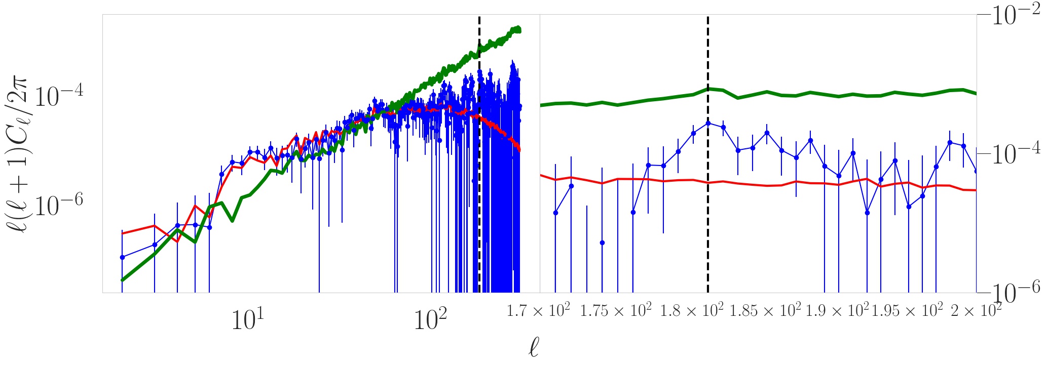
Figure 13: Plots using GMCA with $n_{r}$ = 3 and 400 realizations. The top plot is for 5th channel ($\nu$ = 4), and the bottom one for 13th channel ($\nu$ = 12). On the left plots are multipoles between 2-300, and on the right, between 30-100. The reconstructed HI angular power spectrum and the original one are represented by blue and red colors, respectively. The green color represents the white noise angular power spectrum. The vertical black dashed line corresponds to the multipole 47 (top plots) and 181 (bottom plots).

The estimation of the 21 cm angular power spectrum for the first, tenth, twentieth, and thirtieth channels can be seen in Appendix A for all algorithms (blue color), with respective angular power spectrum from fiducial maps (red color), and white noise angular power spectrum (green color). Here, we will concentrate on quantifying the results. Analyzing the $\chi^{2}$ for 400 simulations to estimate the values, in Fig. 12 there is a heatmap representation where the redder color represents more difficulty to estimate the angular power spectrum value. There are some regions where there are highlighted redder values, as around $(\nu,\ell)=(4,47)$ and $(12,181)$, represented on the top and bottom in Fig. 13, respectively. These plots explicitly show the effect of the lower signal-noise ratio in view of the short observation in time (one year). The top plot has the right representation where the estimated signal follows up the noise bump. The bottom plot shows the same effect, but for the signal-noise relation even lower. Another crucial point to highlight is that only cosmic variance contributes to noise here, leading to further difficulty in obtaining a better $\chi^{2}$ value.

In the Fig. 14 the very similar result for GMCA and FastICA is clear. At the bottom of the figure, we show the percentage ratio between the latest algorithms, where there is no statistical difference between them. But if we see Fig. 19, it shows the estimation of the ninth channel and shows that the algorithms do not work equally to estimate the foreground contribution. In that figure, GMCA and FastICA were run with three non-physical templates for estimating the foreground. We compared the input foreground maps with the estimated one for each algorithm (upper plots) and their respective residuals (central plots). The bottom right plot in that figure represents the difference between GMCA and FastICA estimation. It is possible to see that there are big differences where the foreground emission is higher. FastICA foreground estimation is slightly higher in the Galactic region. Fig. 20 shows the residuals for each algorithm, and it is possible to see a slight difference between them.

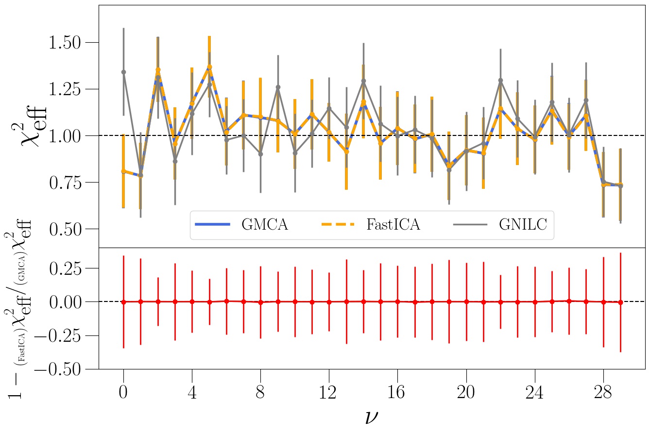
Figure 14: At the top, there is a comparison of effective $\chi^{2}$ of the GMCA (solid blue line), FastICA (dashed orange line), and GNILC (solid gray line). At the bottom, we represent the residual difference between the effective $\chi^{2}$ of FastICA and GMCA.

	GMCA	FastICA	GNILC
GMCA	0	0.00(5)	-0.02(6)
FastICA	0.00(5)	0	-0.02(6)
GNILC	0.02(6)	0.02(6)	0

Table 3: Measuring the difference of Akaike Information Criterium (AIC) from two methods ($\Delta\textrm{AIC}$) is here equivalent to measuring the difference of their overall chi-square. $\Delta\textrm{AIC}>0$ is evidence in favor of the higher chi-square. Comparing the three methods two-by-two and obtaining their errors using Jackknife technique results in all compatibility with 0.

Again, there is no difference between the studied algorithms in our configuration. They are statistically compatible. What is better expressed by the Table 3, that is, the difference between AIC of the algorithms for the last assumed configuration. The values in the table are

$$\Delta\textrm{AIC}_{jk}={}_{\left(M_{j}\right)}^{\left(L_{i}\right)}\chi^{2}_{\textrm{overall}}-{}_{\left(M_{k}\right)}^{\left(L_{i}\right)}\chi^{2}_{\textrm{overall}},$$ (26)

where $j$ is the result from $M_{j}$ algorithm and represents the algorithm in the row, $k$ is the same but for the column. $L_{i}$ is a specific realization chosen. $\Delta\textrm{AIC}_{jk}>0$, which can be represented as ”evidence in favor” of the algorithm $M_{j}$, compared to the $M_{k}$ algorithm. The table presents no evidence in favor of any of the algorithms

We used a Intel(R) Xeon(R) CPU E5-2640 v4 @ 2.40GHz and in relation to computational costs, FastICA is the most efficient among them taking less than one minute per run. While, the GMCA and GNILC take between 6-10 minutes.

7.4 Influence of binned multipoles

Another important information is how binning of the multipoles affects the estimation. Binning helps compressing data and turns all processes faster. However we have an accurate description of how our choice behavior is essential. Binning here is when we take the weighted average of the angular power spectrum per range of the multipoles,

$$\hat{C}_{\Delta\ell_{i}}=\frac{\sum_{\ell\in{\Delta\ell}_{i}}\left(2\ell+1\right)\hat{C}_{\ell}}{\sum_{\ell\in{\Delta\ell_{i}}}\left(2\ell+1\right)},$$ (27)

where $\Delta\ell_{i}$ is $i$th multipole bin that can be of different widths.

We calculated binning effect on the estimation using FastICA with 400 simulations and $n_{s}=3$. Each bin size, minimum and maximum multipoles, number of the multipoles used, and respective $\chi^{2}_{\textrm{overall}}$ are in Table 4.

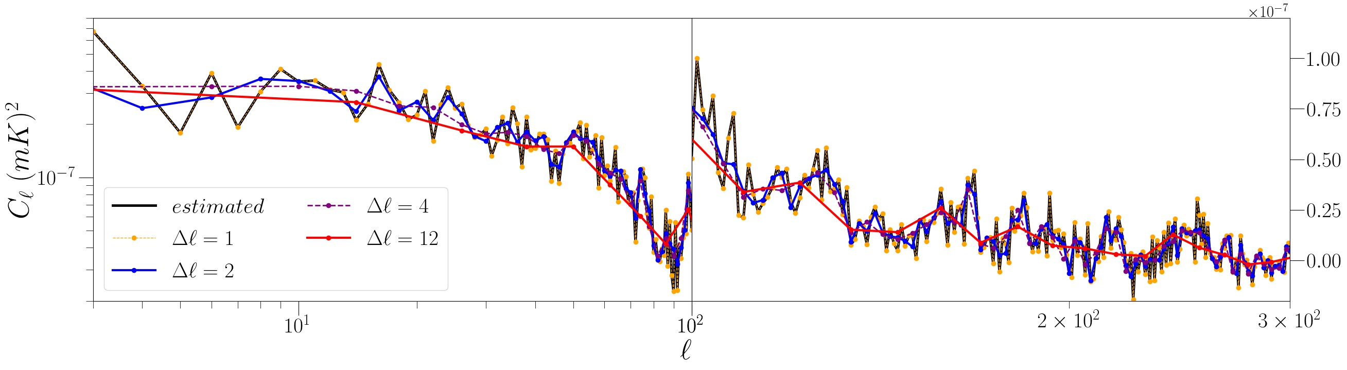
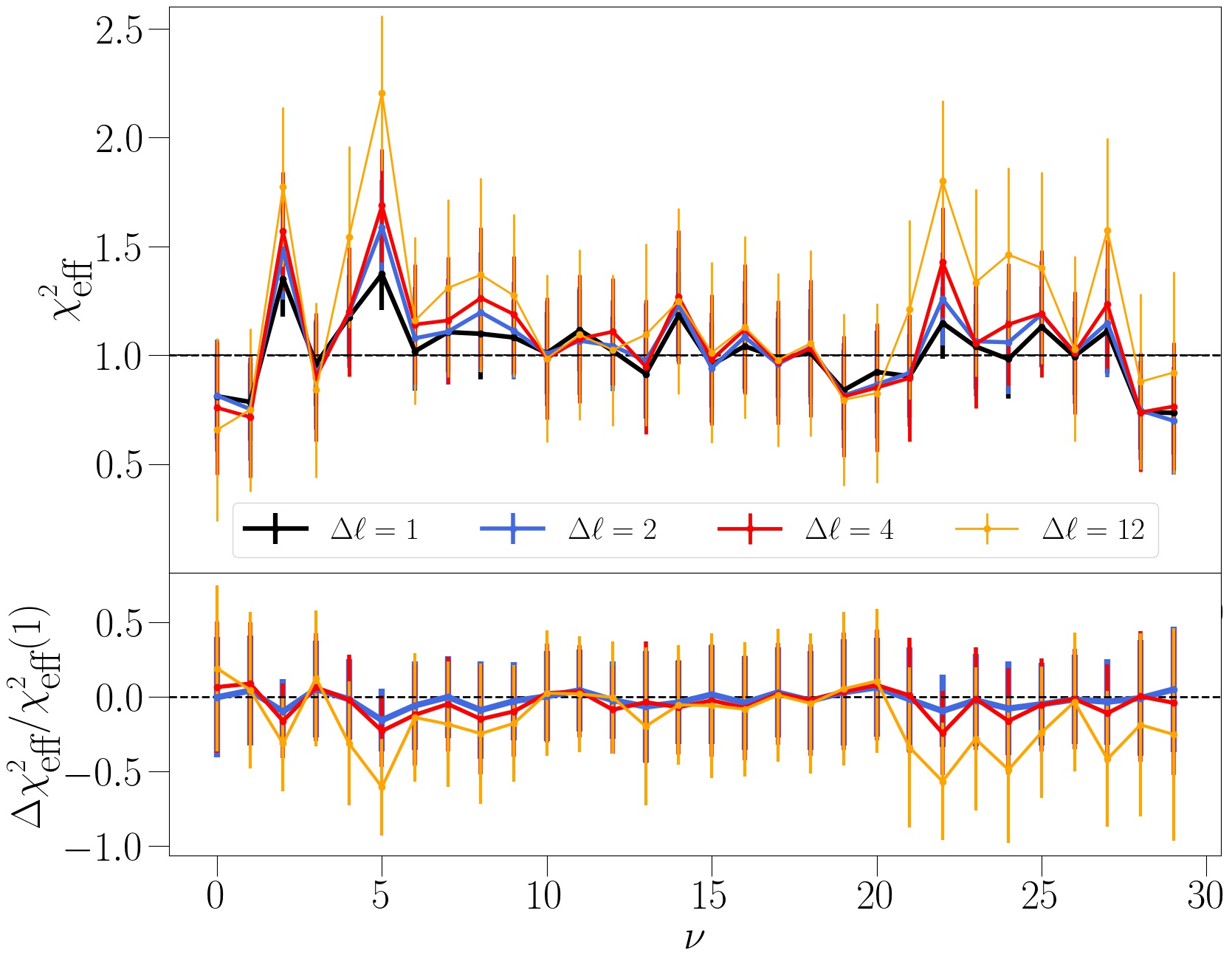
Figure 15: The upper left and right plots correspond to the reconstructed HI angular power spectrum with and without using the function for compressing data. In solid black color is the reconstructed HI without using the process of binning. In the dotted orange line is the HI angular power spectrum for the binning length equal to one (which should be the same as the previous one). The other lines correspond to the binning lengths 2 (blue), 4 (purple), and 12 (red). The bottom center plots are the $\chi^{2}_{\textrm{eff}}$ for HI angular power spectrum through the function for compressing data and the residual difference with the length equal to one.

Fig. 15 represents (top left) the first one hundred angular power spectrum, and (top right) between multipoles 100 and 300, to estimate values with all multipoles and for different $\Delta\ell$. At the bottom, are evaluation of the $\chi^{2}_{\textrm{eff}}$ and their relative difference concerning $\Delta\ell=1$. It is possible to see that there are high shifts of the values for $\Delta\ell=12$ mainly for lower and higher channels. Examining $\chi^{2}_{\textrm{overall}}$ it is possible to identify inconsistency of this binning with in one to two sigmas. By Table. 5, we can see at one sigma level the evidence to $\Delta\ell=1$ and $2$ comparing to $12$. Among 1, 2, and 4, there is no statistical evidence in favor of any choice. Therefore, between $\Delta\ell=1$ and $4$, it has 765 and 191 multipoles - that is, the last is four times smaller - there is no statistical evidence in favor of using each other and $\Delta\ell=4$ is compatible with $\chi^{2}_{\textrm{overall}}=1$ up two sigmas.

$\Delta_{\ell}$	$\ell_{\textrm{min}}$	$\ell_{\textrm{max}}$	$n_{\ell}$	$\chi^{2}_{\textrm{overall}}$
1	2	766	765	1.02(4)
2	2	764	382	1.05(5)
4	2	762	191	1.07(6)
12	2	746	63	1.19(8)

Table 4: Overall chi-square for different lengths of multipole binning through FastICA with 400 realizations and dimension of mixing matrix of 3.

$\Delta\ell$	1	2	4	12
1	0	-0.03(6)	-0.05(7)	-0.17(9)
2	0.03(6)	0	-0.03(7)	-0.15(9)
4	0.05(7)	0.03(7)	0	-0.1(1)
12	0.17(9)	0.15(9)	0.1(1)	0

Table 5: Difference of AIC ($\Delta\textrm{AIC}$) of different multipole binning. Each table value resulted from difference of both row and column overall chi-square multipole binning, with error estimated from Jackknife method between different realizations.

8 Discussions and Conclusions

Our original aim was to build a module of foreground removal and 21 cm estimation for BINGO pipeline that could be user-friendly and flexible enough to explore different methods and mathematical domains, as well as connectable to other modules of the BINGO data analysis pipelines. The next step was to test different module configurations to compare the previous situations and frameworks. This paper results from this second step and the first tests, comparing blind algorithms already implemented. So far, the works on 21 cm post-reionization in the BINGO configuration were published using only GNILC. This work is the first to add new foreground removal methods and compare their performance in the current status of the pipeline. It is a natural result of the BINGO pipeline construction. We investigated three blind foreground removal algorithms applied to BINGO Telescope configuration. It is essential to keep in mind that our analysis did not assume effects from instrumental noise different from white noise. Effects due to the construction of the mirrors lead to changes on the main beam and its side lobes and dependence of the beam with frequency and feed horn location. All of this additional information will be done elsewhere.

In the literature, there are reports of similar behavior between GMCA and ICA-based algorithms (Bobin et al., 2007; Cunnington et al., 2021), and the necessity of a more accurate measure to identify a distinction between them. Here, we could see that both algorithms converge to the equivalent results when which used optimal configuration, but there is a visible difference between them. A possibility for future work is to analyze if the property explored by each algorithm (statistical independence and sparsity) are relevant to the point that can help us identifying foreground contribution. The covered region and the bandwidth assumed can also be influenced in that case. Otherwise, introducing other realistic instrumental effects as correlated band noise, side lobes, realistic non-symmetric main beam, different beams per feed horn, and frequency leads to a more subtle problem beyond our scope. Introducing these effects will change how each algorithm and in which assumed space one is working. Different shapes of the beams per channel and focal plane position are better treated in harmonic space (where GNILC works) than pixel space (FastICA). Assuming only thermal noise as instrumental noise and one year of BINGO coverage, we can get the first study to perform and check possible initial difficulties, and check exactly how each algorithm works in a first and preliminary situation. In one year of the coverage, the 21 cm signal collected cannot be enough to have a good statistics, mainly because the signal-to-noise ratio is still low. This could be seen in Fig. 12 and in Fig. 13, where a higher $\chi^{2}$ value is associated with a higher value of the thermal noise signal even for multipole not really high.

Upon checking $\chi^{2}_{\textrm{eff}}$ for GMCA and FastICA, we learn that the mean value per channel is better described assuming three non-physical templates (Table 1). What is explained by there are three main foreground components stronger in the BINGO region. Now, for different simulations, it is possible to see that GMCA and FastICA converge to the equivalence values for 400 simulations with $n_{s}=3$. That is, possibly both converge to the equivalent values in their optimal case. Finally, comparing three algorithms no significant difference in this pipeline step shows up. Comparisons between all algorithms with $\Delta\textrm{AIC}$ are compatible with zero. That is, there is no any preference for any algorithm.

Again, in this step of the pipeline, it is essential to do many simulations and tests, and for that use, a faster algorithm saves time. Therefore, FastICA can be justified by its easier and faster work without losing information. Each run with FastICA takes less than one minute in a Intel(R) Xeon(R) CPU E5-2640 v4 2.40GHz in 64 bits. While the GMCA and GNILC take between 6-10 minutes. Also, binning the $C_{\ell}$ with $\Delta\ell=2$ reduces the number of multipoles to half and maintains statistical quality.

Lastly, the results got in this step of the pipeline help us better understanding the influence of thermal noise for one year of coverage and compare the three blind algorithms to estimate foreground contribution to the coverage sky. All algorithms are statistically equivalent in this step, what we can explore to use the fastest one. However, we should keep in mind that for more complex foreground models and instrument models, one of the algorithms may perform better than another one. Especially, if there are significant variations of the foreground properties inside the BINGO region, a constant global $n_{s}=3$ value over all pixels like what is assumed by FastICA may lead to poorer results. Also, using a set of angular power spectrum binned with $\Delta\ell=2$ reduces to half the number of multipoles values and maintains the statistical information.

Appendix A Estimated HI angular power spectrum

The accuracy of the HI reconstruction strongly depends on different things: number and type of foregrounds, type of instrumental noises, beam shape, map resolutions, sidelobe effects, polarization leakage, channel, signal-to-noise ratio, the algorithm used to estimate foregrounds, number of simulations in noise debias process, among others.

In this work, we have assumed all maps at equal resolution (40 arcmins) with a Gaussian beam, five foreground sources (section), only white noise as instrumental noise, no polarization leakage and sidelobe effects, three different algorithms, and up to 400 simulations.

We represent the reconstruction of each algorithm with 400 realizations for four different channels (first, 10th, 20th, and 30th channel) in Fig. 16 (GMCA), 17 (GNILC), and 18 (FastICA). GMCA and FastICA using $n_{r}=3$

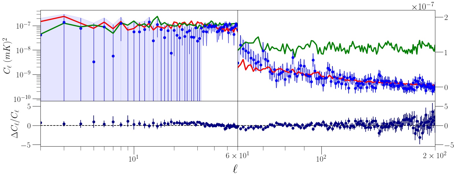
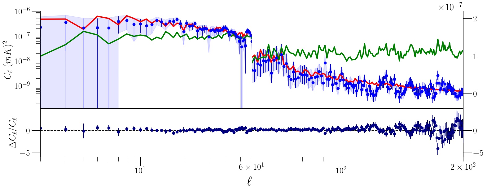
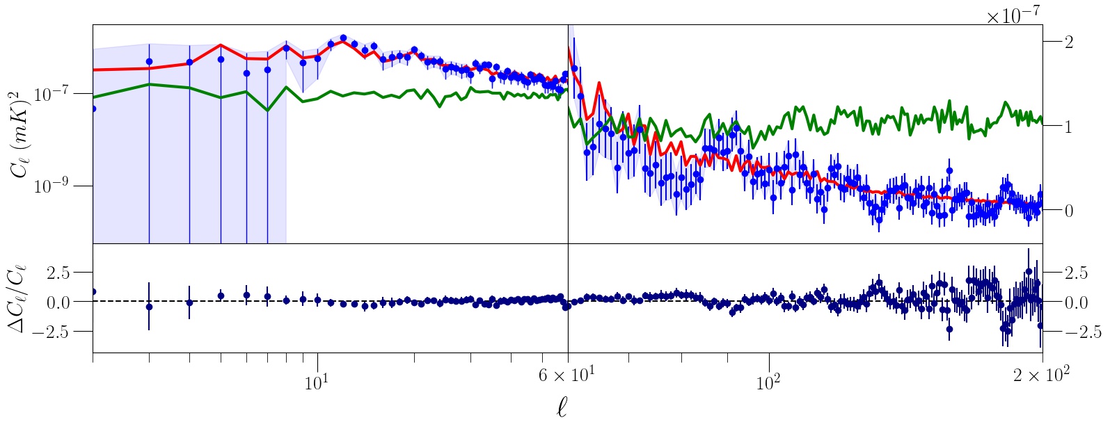
Figure 16: The graphs are the reconstructed HI angular power spectrum for the first (top left), 10th (top right), 20th (bottom left), and 30th (bottom right) channels using GMCA with 400 realizations and $n_{s}$=3. The blue color line represents the HI information reconstructed, the original information in red color, and the white noise information in green color. Below each graph is the residual difference between reconstructed and original HI information.

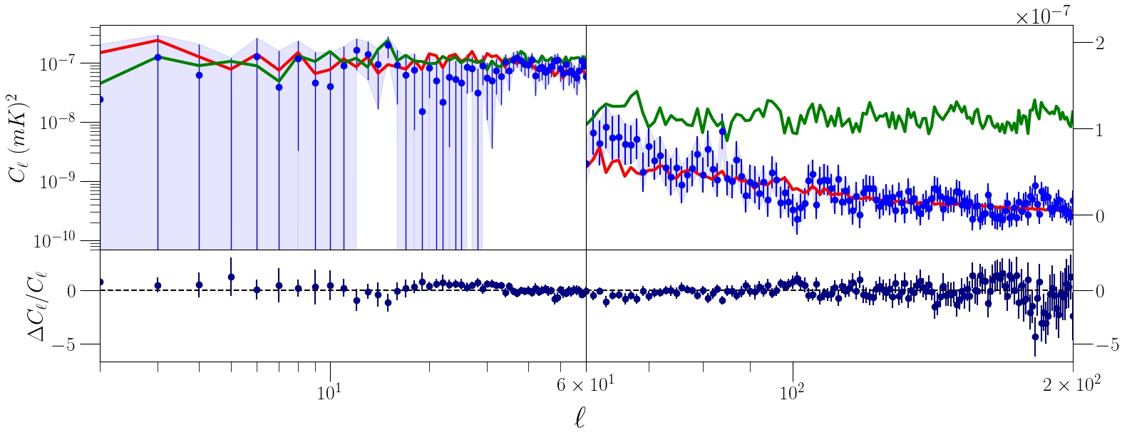
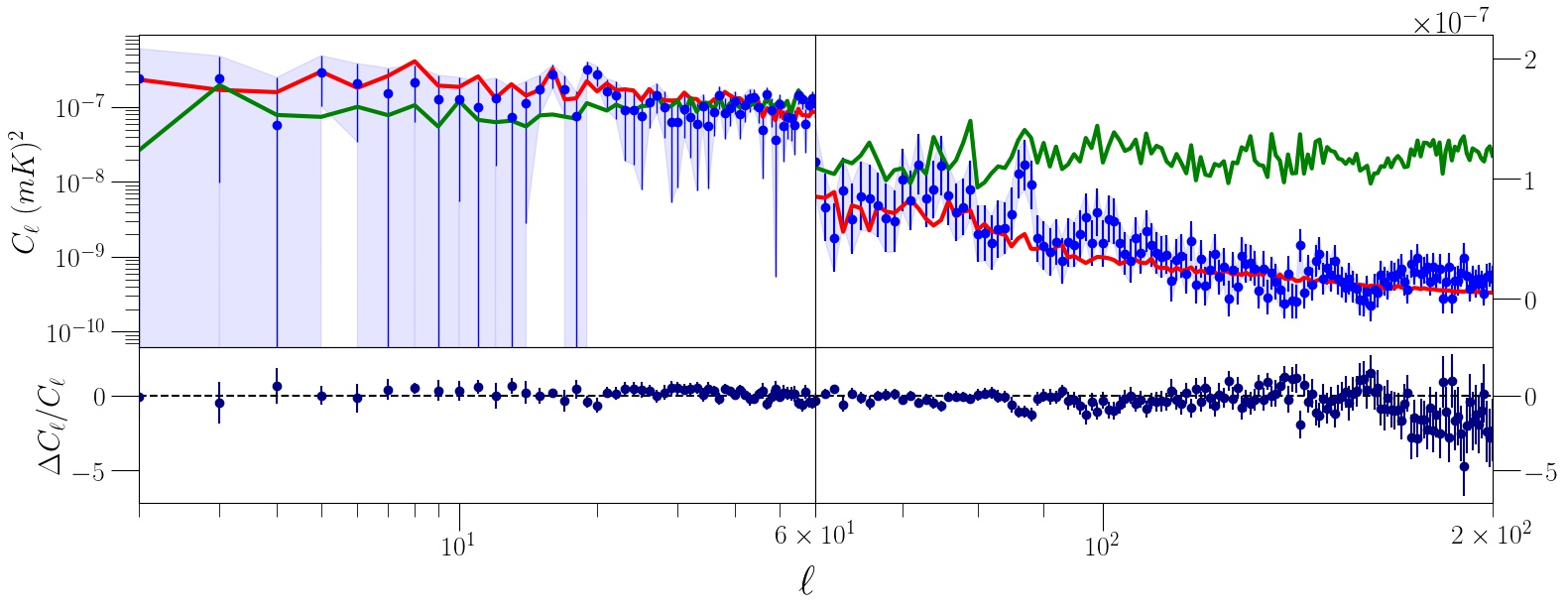
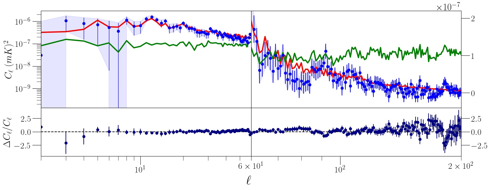
Figure 17: The graphs are the reconstructed HI angular power spectrum for the first (top left), 10th (top right), 20th (bottom left), and 30th (bottom right) channels using GNILC with 400 realizations. The blue color line represents the HI information reconstructed, the original information in red color, and the white noise information in green color. Below each graph is the residual difference between reconstructed and original HI information.

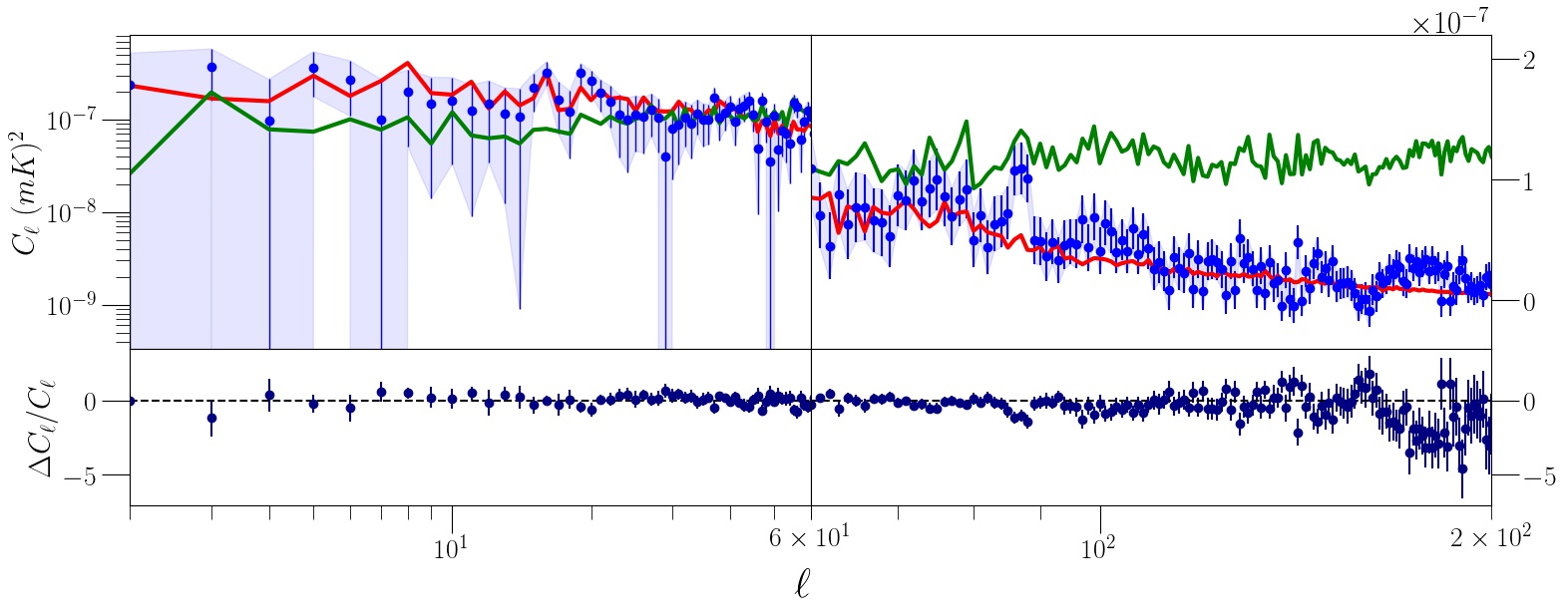
Figure 18: The graphs are the reconstructed HI angular power spectrum for the first (top left), 10th (top right), 20th (bottom left), and 30th (bottom right) channels using FastICA with 400 realizations and $n_{s}$=3. The blue color line represents the HI information reconstructed, the original information in red color, and the white noise information in green color. Below each graph is the residual difference between reconstructed and original HI information.

Appendix B Comparison of GMCA and FastICA maps

Similar results obtained by GMCA and ICA algorithm have been published before. The exact reason behind the similar results is not clear yet. This similarity explains the indifference in starlet or real space results in this work. Although we have shown the statistical equivalence between the algorithms, their results for just one realization are not the same.

In Fig 19, we represent the reconstructed foreground emission by algorithms e their comparisons. The reconstructions are worse at the edge of the mask and in the Galaxy region. The unmasked Galaxy part represents a poor estimate by both algorithms. When we look at the reconstructions one by one, it looks the same, but when we look at the difference between them (bottom-right image), we can see a subtle difference in the Galaxy region.

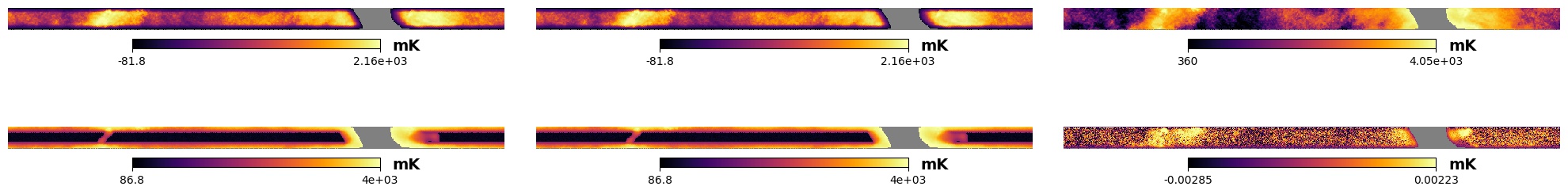
Figure 19: In the first row, there are the foreground emissions reconstructed by (top left) FastICA and (top center) GMCA and the (top right) original foreground emissions. In the plots below, we compare the quality of reconstruction, and the difference between algorithm reconstruction: (bottom left) original subtracted by GMCA reconstructed, (bottom center) original subtracted by FastICA reconstructed, and GMCA minus the FastICA result.

Fig. 20 shows the residual of the algorithms. When we compare the residual from both algorithms (on the right), we can see that in the Galaxy region, there are negative values. These are the same regions with positive difference in Fig 19. Therefore, the GMCA is subtly underestimating emissions from the Galaxy region.

Figure 20: The plots represent the algorithm residuals, (left) FastICA and (right) GMCA, and the (bottom center) difference between both residuals. All maps are of channel 9.

References

- Abdalla et al. (2022a) Abdalla, E., Ferreira, E. G. M., Landim, R. G., et al. 2022a, A&A, 664, A14
- Abdalla et al. (2022b) Abdalla, F. B., Marins, A., Motta, P., et al. 2022b, A&A, 664, A16
- Akaike (1974) Akaike, H. 1974, IEEE Transactions on Automatic Control, 19, 716
- Basak & Delabrouille (2013) Basak, S. & Delabrouille, J. 2013, MNRAS, 435, 18
- Bird et al. (2014) Bird, S., Vogelsberger, M., Haehnelt, M., et al. 2014, Monthly Notices of the Royal Astronomical Society, 445, 2313
- Bobin et al. (2006) Bobin, J., Moudden, Y., Starck, J.-L., Fadili, J. M., & Aghanim, N. 2006, in Astronomical Data Analysis ADA’06, Marseille, France
- Bobin et al. (2007) Bobin, J., Starck, J.-L., Fadili, J., & Moudden, Y. 2007, IEEE Transactions on Image Processing, 16, 2662
- Bozdogan (1987) Bozdogan, H. 1987, Psychometrika, 52, 345
- Carucci et al. (2020) Carucci, I. P., Irfan, M. O., & Bobin, J. 2020, Monthly Notices of the Royal Astronomical Society, 499, 304
- Chapman et al. (2012) Chapman, E., Abdalla, F. B., Harker, G., et al. 2012, MNRAS, 423, 2518
- Chapman & Jelić (2019) Chapman, E. & Jelić, V. 2019, arXiv preprint arXiv:1909.12369
- Chen & Donoho (1995) Chen, S. & Donoho, D. L. 1995, in Society of Photo-Optical Instrumentation Engineers (SPIE) Conference Series, Vol. 2569, Wavelet Applications in Signal and Image Processing III, ed. A. F. Laine, M. A. Unser, & M. V. Wickerhauser, 564–574
- Chen et al. (2001) Chen, S. S., Donoho, D. L., & Saunders, M. A. 2001, SIAM Review, 43, 129
- Costa et al. (2022) Costa, A. A., Landim, R. G., Novaes, C. P., et al. 2022, A&A, 664, A20
- Cunnington et al. (2021) Cunnington, S., Irfan, M. O., Carucci, I. P., Pourtsidou, A., & Bobin, J. 2021, Monthly Notices of the Royal Astronomical Society, 504, 208
- Delabrouille et al. (2013) Delabrouille, J., Betoule, M., Melin, J. B., et al. 2013, A&A, 553, A96