Radiation from Axion star-Neutron star binaries with a tilted rotation axis in the presence of plasma

Abstract

We investigate the form of the radiation emitted by an axion star-neutron star binary using a $f(r)=\text{sech(r/R)}$ profile for the axion star. Our analysis takes into account the co-rotating plasma of the neutron star. We find that that there is significant enhancement to the radiated power if the neutron star’s spin is tilted towards the plane of the axion star-neutron star orbit, compared to the case where it is perpendicular. We also examine whether the neutron star’s co-rotating plasma can play a role in the emitted power and we find that even though dilute axion stars can in principle radiate more efficiently than dense axion stars, they will be pulled apart by the tidal forces of the neutron star

1 Introduction

The axion, initially proposed as a solution to the strong CP problem Peccei and Quinn [1977], Weinberg [1978], is now one of the most well-motivated candidates of dark matter Preskill et al. [1983], Abbott and Sikivie [1983], Dine and Fischler [1983]. The axions are stable bosons, with large occupation numbers and can rethermalize through their gravitational interactions forming a Bose-Einstein condensate (BEC) Sikivie and Yang [2009], Erken et al. [2012]. Owing to the large occupation number of the ground state, the BEC condensate has been treated classically as a localised, coherently oscillating clump called an axion star, if the kinetic pressure is balanced by gravity and axiton or oscillon, if it is balanced by self-interactions. Braaten et al. [2016], Eby et al. [2016a, b], Levkov et al. [2017], Feinblum and McKinley [1968], Chavanis [2018], Visinelli et al. [2018].

The interaction of axions with electromagnetic field has been proposed as a venue for their detection Sikivie [1983]. Of particular interest it the Primakoff effect Primakoff [1951], which is the interaction of an axion with a virtual photon to produce a real photon. One possible "laboratory" that exploits this effect for the detection of the axion is that of neutron stars, where some of the strongest magnetic fields in nature can be found Pshirkov and Popov [2009].

The interaction between a dilute axion star (AS) and a neutron star (NS) has also been proposed to explain Fast Radio Bursts Lorimer et al. [2007], Keane et al. [2010], Thornton et al. [2013], Spitler et al. [2014], where the magnetic field of the neutron star induces an electric field in the axion star which then accelerates electrons in the atmosphere of the neutron star Iwazaki [2015] or induces a dipole moment in neutrons on the upper upper core of the neutron star Raby [2016]. However, due to tidal forces, the AS will break apart in a time scale of the order of seconds, much longer than the millisecond duration of FRBs Pshirkov [2017]. It has been pointed out though that the axion to photon conversion in the collision of an dense AS with a NS may still be able to explain FRBs Buckley et al. [2021], Bai and Hamada [2018].

Recently, the electromagnetic power emitted by an AS-NS binary system was derived analytically Kouvaris et al. [2022]. It was assumed that the AS is described by an exponential profile, that the axis of rotation of the NS is perpendicular to the AS-NS plane and that plasma effects were negligible due to the low frequency of the plasma. For circular orbits, it was found that the spectral flux density of the emitted radiation is modulated mainly by the high frequency spin of the NS. There is also significant enhancement of emitted radiation for elliptical orbits due to the periodic approach of the AS to the NS.

In this work, we include the plasma co-rotating with the NS through the equation $k=\sqrt{\omega^{2}-\omega^{2}_{p}}$, where k is the wave-number of the photon, $\omega$ is its frequency and $\omega_{p}$ is the plasma frequency. We also assume that the rotation axis of the neutron star has a tilt with respect to the the normal to the NS-AS plane, use a profile for the AS that is more accurate than the exponential in the case of attractive self-interactions Eby et al. [2018] and allows us to compare with previous works where a constant magnetic field was assumed Amin et al. [2021], and finally explore the relevance of plasma effects when we consider an axion mass $m_{a}\sim\omega_{p}$.

The paper is organised as follows: In section 2, we review the interactions between the axion and electromagnetism. In section 3, we establish the profile of the axion star that we will be using and describe the magnetic field of the pulsar. In section 4, we calculate the power emitted by the axion condensate and provide analytic formulae. In section 5, we summarise the results of this paper with some remarks for future research.

2 Axion Electrodynamics

The Lagrangian of the axion field coupled to electromagnetism is:

$$\mathcal{L}=\frac{1}{2}\partial_{\mu}\partial^{\mu}\varphi-\frac{1}{2}m^{2}_{\varphi}\varphi^{2}-\frac{1}{4}F_{\mu\nu}F^{\mu\nu}-\frac{g_{a\gamma}}{4}\varphi F_{\mu\nu}\tilde{F}^{\mu\nu}$$ (1)

where $\phi$ is the scalar field of the axion and:

$$F_{\mu\nu}=\partial_{\mu}A_{\nu}-\partial_{\nu}A_{\mu}\,,\qquad\tilde{F^{\mu\nu}}=\frac{1}{2}\epsilon^{\mu\nu\rho\sigma}F_{\rho\sigma}$$ (2)

Note that in the above Lagrangian we have neglected gravity and assumed that there are no free currents and charges. Since the occupation number of the axion field is huge, we may treat its field as a classical field. The equations of motion are:

$$(\Box+m^{2}_{a})\varphi= g_{a\gamma}\bf{E}\cdot\bf{B}$$ (3a)

$$\nabla\cdot\bf{E} =\rho$$ (3b)

$$\nabla\times\bf{B}-\pdv{\bf{E}} =\bf{J}$$ (3c)

$$\nabla\cdot\bf{B} =0$$ (3d)

$$\nabla\times\bf{E}+\pdv{\bf{B}}{t} =0$$ (3e)

where the charge density $\rho$ and current density $\bf{J}$ are:

$$\rho =-g_{a\gamma}\nabla\varphi\cdot\textbf{B}$$ (3da)

J $$=g_{a\gamma}(\pdv{\varphi}{t}\textbf{B}+\nabla\varphi\times\textbf{E})$$ (3db)

This is a set of coupled, partial differential equations. To make progress, we follow Amin et al. [2021] and expand the electromagnetic fields, charge density and current density in the small parameter $g_{a\gamma}\varphi_{0}$:

$$\bf{E}=\bf{E}^{(0)}+\bf{E}^{(1)}+...,\qquad\bf{B}=\bf{B}^{(0)}+\bf{B}^{(1)}+...$$ (3ea)

where $\bf{E}^{(0)}$ and $\bf{B}^{(0)}$ are the background fields that mix with the axion field. The 2 dynamical Maxwell equations for the first order electromagnetic fields are:

$$\nabla\cdot\textbf{E}^{(1)} =\rho^{(1)},$$ (3fa)

$$\nabla\times\textbf{B}^{(1)}-\pdv{\textbf{E}^{(1)}}{t} =\textbf{J}^{(1)}$$ (3fb)

Introducing now the vector and scalar potential through the standard equations $\textbf{B}^{(1)}=\nabla\times\textbf{A}$, $\textbf{E}^{(1)}=-\nabla A^{0}-\pdv{\bf{A}}{t}$, our problem is reduced to calculating $A^{0}$ and A from the equations:

$$(-\nabla^{2}+\frac{\partial^{2}}{\partial t^{2}})A^{0}=\rho$$ (3ga)

$$(-\nabla^{2}+\frac{\partial^{2}}{\partial t^{2}})\textbf{A}=\textbf{J}^{(1)}$$ (3gb)

We now turn to the field of the AS and the background fields $\textbf{E}^{(0)}$ and $\textbf{B}^{(0)}$ of the NS.

3 Axions stars and Neutron stars

3.1 Axion stars

For the axion star, we use the Ansatz proposed in Schiappacasse and Hertzberg [2018] for a spherical symmetric star, oscillating coherently with frequency $\omega$:

$$\varphi=\varphi_{0}f(r)cos(\omega t)$$ (3h)

For the non-relativistic case that we examine here, we may set $\omega=m_{a}$. The spatial profile $f(r)$ must satisfy the boundary condition $f(r)\xrightarrow[]{}0$ when $r\xrightarrow[]{}\infty$ and have an inverted parabola at $r=0$. We will consider the profile:

$$f(r)=\text{sech}(r/R)$$ (3i)

Although we should include a polynomial that captures the behaviour of the field at $r\xrightarrow[]{}0$, these profiles give us the correct qualitative behaviour of the field. It was found in Visinelli et al. [2018], where the potential considered was that of the QCD axion:

$$V(\varphi)=\Lambda^{4}(1-cos(\varphi/f_{a}))$$ (3j)

that if $|\varphi_{0}|\ll f_{a}\,(\frac{10^{-6}eV}{m_{a}})$, where $f_{a}$ is the axion decay constant, we are in the diluted, stable branch where $R\omega\gg 1$ and we can ignore the self-interactions. In this regime, the axion star is supported by its kinetic pressure acting against gravity. Its typical mass and radius is Chavanis [2018], Visinelli et al. [2018]:

$$M_{dilute} \leq 1.0\times 10^{-9}M_{\odot}\left(\frac{f_{a}}{10^{13}\,\text{GeV}}\right)\left(\frac{10^{-6}\,\text{eV}}{m_{a}}\right)$$ (3k)

$$R_{dilute} =27km\left(\frac{10^{13}\,\text{GeV}}{f_{a}}\right)\left(\frac{10^{-6}\,\text{eV}}{m_{a}}\right)$$ (3l)

If $|\varphi_{0}|=\mathcal{O}(1)f_{a}$, we are in the dense branch where $R\geq$few$\times\omega^{-1}$ and we have to include the self-interactions, while the non-relativistic approximation breaks down and our Ansatz 3h does not capture the correct profile of the oscillon. In addition, its lifetime was determined to be short, of the order $\mathcal{O}(\frac{10^{3}}{m})$ and therefore not relevant to cosmological investigations. The radius of a dense axion star is given by Braaten et al. [2016]:

$$R_{dense}=3m\times\left(\frac{10^{13}\,\text{GeV}}{f_{a}}\right)^{1/2}\left(\frac{10^{-6}\,\text{eV}}{m_{a}}\right)^{1/2}\left(\frac{M_{dense}}{10^{-12}M_{\odot}}\right)^{0.3}$$ (3m)

In Zhang et al. [2020], Ollé et al. [2020], Cyncynates and Giurgica-Tiron [2021], in addition to 3j, a number of other potentials were studied and the lifetime of oscillons was found to be up to 5 orders of magnitude larger. However, they arrived to similar results regarding the single frequency approximation i.e. we need a more sophisticated profile than 3h to study dense oscillons-axion stars. In this work, we will assume that the profile in 3h is also correct for dense axion stars and leave a multiple frequency profile for future work.

3.2 Neutron Stars

We are modelling the neutron star as a rotating magnetic dipole of angular frequency $\Omega$ surrounded by co-rotating plasma. In the near zone $r\ll\frac{1}{\Omega}$ the magnetic field is given by:

$$\textbf{B}_{NS}=\frac{B_{0}}{2}\left(\frac{R_{NS}}{r}\right)^{3}(3(\hat{m}\cdot\hat{r})\hat{r}-\hat{m})$$ (3n)

where $R_{NS}$ is the neutron star’s radius, $B_{0}$ is the intensity of the magnetic field on the neutron star’s surface and $\hat{m}$ is the unit vector in the direction of the magnetic moment. The number density of the electrons was derived by Goldreich and Julian assuming perfect conductivity of the plasma Goldreich and Julian [1969]:

$$n_{c}=\frac{2\bf{\Omega}\cdot\textbf{B}}{e}\frac{1}{1-\Omega^{2}r^{2}\sin^{2}\theta}$$ (3o)

while the plasma frequency is given by:

$$\omega_{p}=\sqrt{\frac{4\pi\alpha n_{c}}{m_{e}}}\approx 10^{-5}\text{eV}\sqrt{\frac{\hat{\Omega}\cdot\textbf{B}}{10^{12}G}\frac{1s}{T_{s}}}$$ (3p)

where $T_{s}$ is the period of the NS.

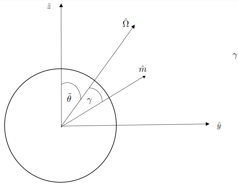
Figure 1: Schematic of the NS showing the different angles. The rotation axis makes a $\tilde{\theta}$ angle with the z axis and the magnetic dipole moment makes a constant $\gamma$ angle with the rotation axis, while precessing around it with $\Omega$ angular frequency

We now turn to the rotation axis of the NS. For simplicity, we will assume that it lies on the y-z plane, at an angle $\tilde{\theta}$ from the z axis:

$$\hat{\Omega}=\begin{pmatrix}0\\ \sin\tilde{\theta}\\ \cos\tilde{\theta}\\ \end{pmatrix}$$ (3q)

We can now perform two successive rotations using SO(3) matrices to obtain the magnetic moment unit vector $\hat{m}$ that precesses around the rotation axis. One is around an axis perpendicular to $\hat{\Omega}$ by an angle $\gamma$ and the next one is around $\hat{\Omega}$ by an angle $\Omega t$. The details are given in Appendix A. Here, we simply write down the final answer:

$$\hat{m}=\begin{pmatrix}\cos(\Omega t)\sin\gamma\\ \cos\gamma\sin\tilde{\theta}+\sin\gamma\cos\tilde{\theta}\sin(\Omega t)\\ \cos\gamma\cos\tilde{\theta}-\sin\gamma\sin\tilde{\theta}\sin(\Omega t)\end{pmatrix}$$ (3r)

Furthermore, we argue that we can ignore the background electric field in 3db. Its value at the surface of the star is $E_{0}$=$B_{0}\Omega a$ and in order to ignore the second term in the right hand side of 3db, it must hold:

$$\nabla\varphi\times\textbf{E}\ll\pdv{\varphi}{t}\textbf{B}\Rightarrow\frac{\textbf{E}_{0}}{R}\ll m_{a}\textbf{B}_{0}\Rightarrow{}\frac{\Omega R_{NS}}{c}\ll m_{a}R$$ (3s)

For typical values of $R_{NS}$=10 km, $\Omega=10^{-3}-1s$, this inequality is true for the range of $m_{a}R$ that we are interested in.

3.3 AS-NS binary

Assuming that $M_{NS}\gg M_{AS}$, we can place the NS in the origin of our coordinate system and the AS will be orbiting around it. The AS’s motion is described by the familiar equation for elliptical orbits:

$$r_{a}=\frac{(1-e^{2})r_{0}}{1+e\cos\phi_{a}},\ r_{0}=\frac{l^{2}_{0}}{GM_{NS}(1-e^{2})}$$ (3t)

where $r_{0}$ is the semi-major axis, $l_{0}$ is the angular momentum per unit mass, $\phi_{a}$ is the azimuthal angle of the AS and $e$ is the eccentricity. We will restrict our analysis to the cases where $e=0$ and $0<e<1$, to circular and elliptical orbits respectively. Since the AS lies on the $x-y$ plane, its position vector is:

$$\textbf{r}_{a}=r_{a}(\cos\phi_{a},\sin\phi_{a},0)$$ (3u)

Later on, we will also need the time dependence of the angle $\phi_{a}$ which is given by the parametric equations Herbert Goldstein [2001]:

$$\omega t=\psi-e\sin\psi,\hskip 5.69046pt\cos\phi_{a}=\frac{\cos\psi-e}{1-e\cos\psi}$$ (3v)

where $0\leq\psi\leq 2\pi$ and $\omega$ is the angular frequency of the AS’s rotation around the NS. The period of rotation is $T_{AS}=\frac{2\pi}{\omega}$, which we will assume to be 10s.

. We will also assume for simplicity that Earth’s position vector lies on the z axis.

$M_{NS}(M_{\odot})$	$M_{dense}(M_{\odot})$	$R_{NS}(km)$	$r_{0}(km)$
1.4	$10^{-12}$	15	$7.8\times 10^{3}$
$\gamma(rad)$	$T_{AS}(s)$	$T_{s}(s)$	$m_{a}(\text{eV})$
0.3	10	1	$10^{-6}$
$f_{a}(\text{GeV})$	$c_{\gamma}$	$r_{e}(kpc)$	$B_{0}(G)$
$10^{14}$	$10^{5}$	1	$10^{12}$

Table 1: A table with the relevant constants of our system

Table 1 summarises the constants relevant to our system, which we take to be the same as in Kouvaris et al. [2022], except for $f_{a}$ which we take to be $f_{a}=10^{13}\text{GeV}$, so that we are consistent with the equation $m_{a}f_{a}=m_{\pi}f_{\pi}=(10^{8}\text{eV})^{2}$ that must be true for the QCD axion.

4 Analytic calculation of emitted power

The radiating fields are given by the known equations:

B $$=\nabla\times\textbf{A},$$ (3ac)

E $$=i\omega\textbf{A}-\nabla A^{0}=\frac{i}{\omega}\left(\omega^{2}\textbf{A}-\textbf{k}(\textbf{k}\cdot\textbf{A})\right)$$ (3ad)

where we have taken the Fourier transform in time and used the Lorentz gauge $\nabla\cdot\textbf{A}+\partial_{0}A^{0}=0$. Here, $|\textbf{k}|=\sqrt{m_{a}^{2}-\omega_{p}^{2}}$. It is therefore sufficient to solve 3gb. Using the retarded Green’s function, the solution is:

$$\textbf{A}(\textbf{r}_{e})=\frac{g_{a\gamma}\varphi_{0}\omega\textbf{B}_{NS}}{4\pi r_{e}}\int d^{3}r^{\prime}e^{ik|\textbf{r}_{e}-\textbf{r}^{\prime}|}\,f(|\textbf{r}^{\prime}-\textbf{r}_{a}|)$$ (3ae)

The magnetic field varies negligibly within the AS, so we can take it out of the integral. We will only write the final result of this integration here and leave the details for Appendix B.

$$\textbf{A}(\textbf{r}_{e})\approx\frac{g_{a\gamma}\varphi_{0}\omega(\pi R)^{2}\textbf{B}_{NS}(\textbf{r}_{a})}{4kr_{e}}\frac{\tanh(\pi kR/2)}{\cosh(\pi kR/2)}e^{ik|\textbf{r}_{e}-\textbf{r}_{a}|}$$ (3af)

The time averaged Poynting vector is given by:

$$\langle\textbf{S}\rangle=\frac{1}{2}\Re(\textbf{E}\times\textbf{B}^{\star})=\frac{1}{2\omega}\Re\left(\textbf{k}(\omega^{2}|\textbf{A}|^{2}-|\textbf{k}\cdot\textbf{A}|^{2})-\omega^{2}_{p}(\textbf{k}\cdot\textbf{A})\textbf{A}^{\star}\right)$$ (3ag)

Inserting in 3ag the expression in 3af, we find for the Poynting vector and the power per solid angle :

$$\langle\textbf{S}\rangle=\frac{\pi^{4}\omega}{32r^{2}_{e}}\left(\frac{g_{a\gamma}\varphi_{0}R^{2}}{k}\right)^{2}\left(\frac{\tanh(\pi kR/2)}{\cosh(\pi kR/2)}\right)^{2}\left(\textbf{k}(\omega^{2}|\textbf{B}_{NS}|^{2}-(\textbf{k}\cdot\textbf{B}_{NS})^{2})-\omega^{2}_{p}\textbf{B}_{NS}(\textbf{k}\cdot\textbf{B}_{NS})\right)$$ (3ah)

$$\frac{dP}{d\Omega}=r^{2}_{e}\hat{k}\cdot\langle\textbf{S}\rangle=\frac{\pi^{4}(g_{a\gamma}\varphi_{0}\omega^{2}R^{2})^{2}}{32k\omega}\left(\frac{\tanh(\pi kR/2)}{\cosh(\pi kR/2)}\right)^{2}|\textbf{B}_{NS}|^{2}\sin^{2}\beta$$ (3ai)

where $\beta$ is the angle between the magnetic field at the AS’s position and Earth’s position vector from the AS. It comes as no surprise that this is the same expression as the one derived in Amin et al. [2021], where a constant magnetic field was assumed.

Figure 2: Plot of the function $\left(\frac{\tanh(\pi\omega R/2)}{\cosh(\pi\omega R/2)}\right)^{2}$ versus $\omega R$. The function has a peak at $\omega R$=0.56 and is exponentially suppressed for $\omega R\gg 1$

.

4.1 AS-NS binary in vacuum

For the benchmark values considered in Table 1, $\omega_{p}\sim 10^{-9}\text{eV}$, so we can neglect plasma effects for the moment, since $m_{a}\sim 10^{-6}\text{eV}$. The power per solid angle, equation 3ai, is exponentially suppressed with respect to $\omega R$, which means that only dense axion stars can radiate efficiently in vacuum. We can understand this by considering energy-momentum conservation in the axion to photon conversion process Sikivie [2021].

Let us examine the conversion rate of axions to photons in the presence of a magnetic field that has only spatial variation, $\textbf{B}_{0}(\textbf{x})$. The conversion rate is proportional to $|\int d^{3}xe^{-i(\textbf{k}-\textbf{k}_{a})\cdot\textbf{x}}\hat{e}_{\lambda}(\hat{n})\cdot\textbf{B}_{0}(\textbf{x})|^{2}$, where $\hat{e}_{\lambda}(\hat{n})$, with $\lambda=1,2$ are the two final state polarization vectors of a photon travelling in the $\hat{n}$ direction, k is the momentum of the photon and $\textbf{k}_{a}$ is the momentum of the axion. A sum over $\lambda$ is implied. Energy conservation is satisfied because $\textbf{B}_{0}(\textbf{x})$ is time-independent. However, the axion satisfies the dispersion relation $\omega=\sqrt{k_{a}^{2}+m_{a}^{2}}$, while the photon satisfies $\omega=|\textbf{k}|$. Thus their momenta will in general be different, but if we decompose the magnetic field into its Fourier modes, $\tilde{\textbf{B}}_{0}(\textbf{q})$, momentum transfer is guaranteed because then $\textbf{q}=\textbf{k}-\textbf{k}_{a}$. In our case, we assumed that the magnetic field is constant within the range of integration, therefore $|\textbf{k}_{a}|\approx\omega\Rightarrow\frac{1}{R}\approx\omega$.

We may define the spectral flux density as $\mathcal{S}=\frac{dP}{d\Omega}\left(r^{2}_{e}\mathcal{B}\right)^{-1}$, where $\mathcal{B}=\frac{0.1m_{a}}{2\pi}$ is an estimate for the Doppler width. Inserting the benchmark values we are considering, the result is:

$$S =2.36\times 10^{-5}\text{Jy}\left(\frac{c_{\gamma}}{10^{5}}\right)^{2}\left(\frac{10^{13}\text{GeV}}{f_{a}}\right)^{2}\left(\frac{10^{-6}\text{eV}}{m_{a}}\right)\left(\frac{M_{dense}}{10^{-12}M_{\odot}}\right)^{1.2}\left(\frac{B_{0}}{10^{12}\text{GeV}}\right)^{2}\times$$

$$\times\left(\frac{1kpc}{r_{e}}\right)^{2}\sin^{2}\beta\left(\frac{1+e\cos\phi_{a}}{1-e^{2}}\right)^{6}|3(\hat{m}\cdot\hat{r})\hat{r}-\hat{m}|^{2}$$ (3aj)

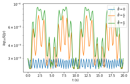
Figure 3: Spectral flux density versus time for e=0. The blue colour represents the rotation axis on the z axis, while orange and green represent the rotation axis at $\tilde{\theta}=\frac{\pi}{4}$ and $\tilde{\theta}=\frac{\pi}{2}$ respectively

In Figure 3, we plot the spectral flux density versus time for three different $\tilde{\theta}$ angles. For $\tilde{\theta}=0$, our results are similar to what was found in Kouvaris et al. [2022] i.e., the signal is modulated by the rotation of the AS around the NS and by the spinning of the NS around its axis. The envelope at the top is approximately flat because the separation between the AS and NS does not change with time. This picture changes if we allow the NS’s rotation axis to be tilted. The position of the AS now plays a more important role in modulating the signal, as we can see from the peaks and troughs in the plot that have a period of 5 seconds. The locations of these maxima and minima can be explained if we remember that the AS starts its orbit on the x axis, where it receives the minimum amount of magnetic field lines from the NS, since the latter’s rotation axis is now on the y-z plane. At 2.5 seconds, the AS has made one quarter of the orbit and it is found on the y-axis, where it now receives the maximum number of magnetic field lines. At 5 seconds, it is on the $x$ axis again, where it receives the minimum amount and so on. We would expect that $S$ would be larger the closer the NS rotation axis is to the x-y plane. This also confirmed by Figure 3, where we see that as $\tilde{\theta}$ increases, $S$ also increases.

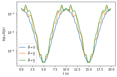
Figure 4: Spectral flux density versus time for e=0.5. The blue color represents the rotation axis on the z axis, while orange and green represent the rotation axis at $\tilde{\theta}=\frac{\pi}{4}$ and $\tilde{\theta}=\frac{\pi}{2}$ respectively

In the case where $e=0.5$, Figure 4, the situation is different, because now the separation between the NS and the AS changes periodically with time. The orbit stars from the perihelion, where the signal is maximum. At 5 seconds, it is on the aphelion, where it is minimum and so on. As it was pointed out in Kouvaris et al. [2022], this is easily explained if we remember that $|\textbf{B}_{NS}|^{2}\sim\frac{1}{r^{6}}$, so there is significant enhancement to the signal if the AS is close to the NS. Hence, the modulation due to the NS spinning is not as important. This is confirmed by our results when we allow the NS’s rotation axis to be tilted. In Figure 4, it is evident that $S$ is slightly enhanced for the cases $\tilde{\theta}=\frac{\pi}{4},\frac{\pi}{2}$, but not by much compared to the $\tilde{\theta}=0$ case.

4.2 AS-NS binary in plasma

We would like to investigate how the plasma surrounding the NS affects the emitted power. To that end, we consider a lower axion mass, of the order $m_{a}=10^{-9}-10^{-8}\text{eV}$. This is outside of the QCD axion range, but it is valid for ALPs, where $f_{a}$ and $m_{a}$ are independent. We will keep the value of $f_{a}=10^{13}\text{GeV}$ for the axion decay constant.

It was shown in Amin et al. [2021] that when $\omega\rightarrow\omega_{p}$, the emitted power per solid angle becomes:

$$\frac{dP}{d\Omega}({\omega\rightarrow\omega_{p}})\approx\frac{(g_{a\gamma}\varphi_{0})^{2}}{128}\frac{(\pi\omega R)^{6}}{\omega^{2}}\left(1-\frac{\omega_{p}^{2}}{\omega^{2}}\right)^{1/2}|\textbf{B}_{NS}|^{2}\sin^{2}\beta$$ (3ak)

There is significant enhancement in power now if $\omega R\gg 1$,due to the factor $(\omega R)^{6}$. Therefore dilute axion stars can radiate much more efficiently than dense axion stars. Inserting in 3k $m_{a}=10^{-9}\text{eV}$, we find for the radius $R_{AS,dilute}=27000\text{km}$ and $M_{AS,dilute}\approx 10^{-6}M_{\odot}$. The Roche limit for this AS is then $R_{Roche}=R_{AS,dilute}\left(\frac{2M_{NS}}{M_{AS.dilute}}\right)^{1/3}\approx 38\times 10^{5}\text{km}$, much larger than the semi-major axis $r_{0}=7.8\times 10^{3}\text{km}$. Hence, even though dilute axion stars could theoretically radiate in the presence of plasma, they will be pulled apart by tidal forces and disintegrate. We tried to avoid this problem by increasing $r_{0}$. However, if we increase $r_{0}$, the plasma frequency, equation 3p, becomes smaller. This means that we have to lower the axion mass too, increasing the AS radius, via equation 3k, leading again to a Roche limit larger than $r_{0}$. It is an open question what happens to the remnants of this disintegrated AS which we leave for future work.

5 Conclusions and Outlook

In this paper, we have derived analytical expressions for the spectral flux density emitted by an AS that is gravitationally bound to a NS. We have used a sech profile to describe the AS that captures its essential characteristics and took into account plasma effects using the Goldreich-Julian model for the NS. We have also allowed the rotation axis of the NS to be tilted towards the plane of the AS-NS, placing it on the y-z plane. If the orbit is circular, we find that there is an order of magnitude increase to the spectral flux density whenever the AS is on the y axis, because of the increased number of magnetic field lines that now pass through the axion star. If, on the other hand, the orbit is an ellipse, there is no significant enhancement to the flux, since now the main modulation comes from the AS’s orbit.

We also considered the effect that the plasma may have on the flux. Given that in the presence of plasma only dilute stars can radiate efficiently, we lowered the axion mass to $m_{a}=10^{-9}\text{eV}$ to investigate this possibility. We found that by lowering the mass, we increase the AS radius, which in turn increases the Roche limit by several orders of magnitude more than the AS-NS distance, meaning that the dilute AS will be torn apart by tidal forces before it interacts with the NS’s magnetic field.

Some interesting venues for future research would be to investigate the effect of back-reaction to the AS profile. This would probably require solving numerically the set of equations 3. Back-reaction could also shed some light to the time scale of disintegration of a dilute AS in the gravitational field of a neutron star or a black hole. Another interesting direction of research would be to include a multi-frequency profile for the dense AS. As it was mentioned in the introduction, given that there have been attempts to explain FRBs with dense axion stars, a more accurate profile for the AS would be a step in that direction.

Appendix A Appendix

We choose the vector perpendicular to $\hat{\Omega}$ to be:

$$\hat{\Omega}_{\perp}=\begin{pmatrix}0\\ -\cos\tilde{\theta}\\ \sin\tilde{\theta}\end{pmatrix}$$ (3al)

The rotation matrix about this vector and by an angle $\gamma$ is given by $R(\hat{\Omega}_{\perp},\gamma)=e^{i\gamma\,\hat{\Omega}_{\perp}\cdot\textbf{L}}$, where L are the generators of SO(3). They are given by:

$$L_{1}=\begin{pmatrix}0&0&0\\ 0&0&-i\\ 0&i&0\\ \end{pmatrix},\ L_{2}=\begin{pmatrix}0&0&i\\ 0&0&0\\ -i&0&0\\ \end{pmatrix},\ L_{3}=\begin{pmatrix}0&-i&0\\ i&0&0\\ 0&0&0\\ \end{pmatrix}$$ (3am)

Using these expressions, we find the rotation matrix to be:

$$R(\hat{\Omega}_{\perp},\gamma)=\begin{pmatrix}\cos\gamma&\sin\tilde{\theta}\sin\gamma&\cos\tilde{\theta}\sin\gamma\\ -\sin\tilde{\theta}\sin\gamma&\cos^{2}\tilde{\theta}+\sin^{2}\tilde{\theta}\cos\gamma&-\sin 2\tilde{\theta}\sin^{2}(\frac{\gamma}{2})\\ -\cos\tilde{\theta}\sin\gamma&-\sin(2\tilde{\theta})\sin^{2}(\frac{\gamma}{2})&\sin^{2}\tilde{\theta}+\cos^{2}\tilde{\theta}\cos\gamma\\ \end{pmatrix}$$ (3an)

As it was mentioned in the text, we now perform a second rotation around $\hat{\Omega}$ by an angle $\Omega t$. The matrix is $R(\hat{\Omega},\Omega t)=e^{-i\,(\Omega t)\,\hat{\Omega}\cdot\textbf{L}}$ and using the generators 3am, we get:

$$R(\hat{\Omega},\Omega t)=\begin{pmatrix}\cos\Omega t&-\cos\tilde{\theta}\sin\Omega t&\sin\tilde{\theta}\sin\Omega t\\ \cos\tilde{\theta}\sin\Omega t&\sin^{2}\tilde{\theta}+\cos^{2}\tilde{\theta}\cos\Omega t&\sin 2\tilde{\theta}\sin^{2}(\frac{\Omega t}{2})\\ -\sin\tilde{\theta}\sin\Omega t&\sin(2\tilde{\theta})\sin^{2}(\frac{\Omega t}{2})&\cos^{2}\tilde{\theta}+\sin^{2}\tilde{\theta}\cos\Omega t\\ \end{pmatrix}$$ (3ao)

Applying these two rotations successively, we obtain the magnetic moment unit vector in equation 3r.

Appendix B Appendix

The integral of equation 3ae is:

$$\mathcal{I}=\int d^{3}r^{\prime}e^{ik|\textbf{r}_{e}-\textbf{r}^{\prime}|}f(|\textbf{r}^{\prime}-\textbf{r}_{a}|)$$ (3ap)

The easiest way to do it is to shift the coordinate system and place in the centre of the AS, $\textbf{r}^{\prime}\rightarrow\textbf{r}_{a}+\textbf{s}$. The exponential can be written as $|\textbf{r}_{e}-\textbf{r}_{a}-\textbf{s}|\approx|\textbf{r}_{e}-\textbf{r}_{a}|-\frac{(\textbf{r}_{e}-\textbf{r}_{a})\cdot\tilde{\textbf{r}}}{|\textbf{r}_{e}-\textbf{r}_{a}|}\approx|\textbf{r}_{e}-\textbf{r}_{a}|-\hat{r}_{e}\cdot\textbf{s}$, where we have assumed that $r_{e}\gg r_{a}$. Of course, $\omega_{p}(r^{\prime})\sim\frac{1}{(r^{\prime})^{3/2}}=\frac{1}{|\textbf{s}+\textbf{r}_{a}|^{3/2}}$. But, because of the exponentially decaying profile $\text{sech}(r/R)$ that we are using for the axion star, the main contribution to the integral 3ap will come from $0<s\lesssim 5R$, much smaller than $r_{a}$. We therefore set $\omega_{p}(r^{\prime})=\omega_{p}(r_{a})$.The angular part of the integral is:

$$2\pi\int^{\pi}_{0}d\theta_{s}\sin\theta_{s}e^{-iks\cos\theta_{s}}=\frac{4\pi\sin(ks)}{ks}$$ (3aq)

while, using the profile $f(r)=\text{sech}(r/R)$, the radial part becomes:

$$\int^{\infty}_{0}ds\,s\,\sin(ks)\,\text{sech}(s/R)=\frac{\pi^{2}R^{2}}{4}\,\frac{\tanh\left(\frac{\pi kR}{2}\right)}{\cosh\left(\frac{kR\pi}{2}\right)}$$ (3ar)

Plugging equations 3aq and 3ar back into 3ap, we get:

$$\mathcal{I}=\frac{\left(\pi R\right)^{3}}{kR}\frac{\tanh\left(\frac{kR\pi}{2}\right)}{\cosh\left(\frac{kR\pi}{2}\right)}e^{ik|\textbf{r}_{e}-\textbf{r}_{a}|}$$ (3as)

which gives equation 3af.

References

- Peccei and Quinn [1977] R. D. Peccei and Helen R. Quinn. conservation in the presence of pseudoparticles. Phys. Rev. Lett., 38:1440–1443, Jun 1977. doi: 10.1103/PhysRevLett.38.1440. URL https://link.aps.org/doi/10.1103/PhysRevLett.38.1440.
- Weinberg [1978] Steven Weinberg. A new light boson? Phys. Rev. Lett., 40:223–226, Jan 1978. doi: 10.1103/PhysRevLett.40.223. URL https://link.aps.org/doi/10.1103/PhysRevLett.40.223.
- Preskill et al. [1983] John Preskill, Mark B. Wise, and Frank Wilczek. Cosmology of the invisible axion. Physics Letters B, 120(1):127–132, 1983. ISSN 0370-2693. doi: https://doi.org/10.1016/0370-2693(83)90637-8. URL https://www.sciencedirect.com/science/article/pii/0370269383906378.
- Abbott and Sikivie [1983] L.F. Abbott and P. Sikivie. A cosmological bound on the invisible axion. Physics Letters B, 120(1):133–136, 1983. ISSN 0370-2693. doi: https://doi.org/10.1016/0370-2693(83)90638-X. URL https://www.sciencedirect.com/science/article/pii/037026938390638X.
- Dine and Fischler [1983] Michael Dine and Willy Fischler. The Not So Harmless Axion. Phys. Lett. B, 120:137–141, 1983. doi: 10.1016/0370-2693(83)90639-1.
- Sikivie and Yang [2009] P. Sikivie and Q. Yang. Bose-einstein condensation of dark matter axions. Physical Review Letters, 103(11), sep 2009. doi: 10.1103/physrevlett.103.111301. URL https://doi.org/10.1103%2Fphysrevlett.103.111301.
- Erken et al. [2012] O. Erken, P. Sikivie, H. Tam, and Q. Yang. Axion dark matter and cosmological parameters. Physical Review Letters, 108(6), feb 2012. doi: 10.1103/physrevlett.108.061304. URL https://doi.org/10.1103%2Fphysrevlett.108.061304.
- Braaten et al. [2016] Eric Braaten, Abhishek Mohapatra, and Hong Zhang. Dense axion stars. Phys. Rev. Lett., 117:121801, Sep 2016. doi: 10.1103/PhysRevLett.117.121801. URL https://link.aps.org/doi/10.1103/PhysRevLett.117.121801.
- Eby et al. [2016a] Joshua Eby, Peter Suranyi, and L. C. R. Wijewardhana. The lifetime of axion stars. Modern Physics Letters A, 31(15):1650090, may 2016a. doi: 10.1142/s0217732316500905. URL https://doi.org/10.1142%2Fs0217732316500905.
- Eby et al. [2016b] Joshua Eby, Madelyn Leembruggen, Peter Suranyi, and L. C. R. Wijewardhana. Collapse of axion stars. Journal of High Energy Physics, 2016(12), dec 2016b. doi: 10.1007/jhep12(2016)066. URL https://doi.org/10.1007%2Fjhep12%282016%29066.
- Levkov et al. [2017] D. G. Levkov, A. G. Panin, and I. I. Tkachev. Relativistic axions from collapsing bose stars. Phys. Rev. Lett., 118:011301, Jan 2017. doi: 10.1103/PhysRevLett.118.011301. URL https://link.aps.org/doi/10.1103/PhysRevLett.118.011301.
- Feinblum and McKinley [1968] David A. Feinblum and William A. McKinley. Stable states of a scalar particle in its own gravational field. Phys. Rev., 168:1445–1450, Apr 1968. doi: 10.1103/PhysRev.168.1445. URL https://link.aps.org/doi/10.1103/PhysRev.168.1445.
- Chavanis [2018] Pierre-Henri Chavanis. Phase transitions between dilute and dense axion stars. Physical Review D, 98(2), jul 2018. doi: 10.1103/physrevd.98.023009. URL https://doi.org/10.1103%2Fphysrevd.98.023009.
- Visinelli et al. [2018] Luca Visinelli, Sebastian Baum, Javier Redondo, Katherine Freese, and Frank Wilczek. Dilute and dense axion stars. Physics Letters B, 777:64–72, 2018. ISSN 0370-2693. doi: https://doi.org/10.1016/j.physletb.2017.12.010. URL https://www.sciencedirect.com/science/article/pii/S0370269317309875.
- Sikivie [1983] P. Sikivie. Experimental tests of the "invisible" axion. Phys. Rev. Lett., 51:1415–1417, Oct 1983. doi: 10.1103/PhysRevLett.51.1415. URL https://link.aps.org/doi/10.1103/PhysRevLett.51.1415.
- Primakoff [1951] H. Primakoff. Photo-production of neutral mesons in nuclear electric fields and the mean life of the neutral meson. Phys. Rev., 81:899–899, Mar 1951. doi: 10.1103/PhysRev.81.899. URL https://link.aps.org/doi/10.1103/PhysRev.81.899.
- Pshirkov and Popov [2009] M. S. Pshirkov and S. B. Popov. Conversion of dark matter axions to photons in magnetospheres of neutron stars. Journal of Experimental and Theoretical Physics, 108(3):384–388, mar 2009. doi: 10.1134/s1063776109030030. URL https://doi.org/10.1134%2Fs1063776109030030.
- Lorimer et al. [2007] D. R. Lorimer, M. Bailes, M. A. McLaughlin, D. J. Narkevic, and F. Crawford. A Bright Millisecond Radio Burst of Extragalactic Origin. Science, 318(5851):777, November 2007. doi: 10.1126/science.1147532.
- Keane et al. [2010] E. F. Keane, D. A. Ludovici, R. P. Eatough, M. Kramer, A. G. Lyne, M. A. McLaughlin, and B. W. Stappers. Further searches for Rotating Radio Transients in the Parkes Multi-beam Pulsar Survey. Monthly Notices of the Royal Astronomical Society, 401(2):1057–1068, 01 2010. ISSN 0035-8711. doi: 10.1111/j.1365-2966.2009.15693.x. URL https://doi.org/10.1111/j.1365-2966.2009.15693.x.
- Thornton et al. [2013] D. Thornton, B. Stappers, M. Bailes, B. Barsdell, S. Bates, N. D. R. Bhat, M. Burgay, S. Burke-Spolaor, D. J. Champion, P. Coster, N. D’Amico, A. Jameson, S. Johnston, M. Keith, M. Kramer, L. Levin, S. Milia, C. Ng, A. Possenti, and W. van Straten. A Population of Fast Radio Bursts at Cosmological Distances. Science, 341(6141):53–56, July 2013. doi: 10.1126/science.1236789.
- Spitler et al. [2014] L. G. Spitler, J. M. Cordes, J. W. T. Hessels, D. R. Lorimer, M. A. McLaughlin, S. Chatterjee, F. Crawford, J. S. Deneva, V. M. Kaspi, R. S. Wharton, B. Allen, S. Bogdanov, A. Brazier, F. Camilo, P. C. C. Freire, F. A. Jenet, C. Karako-Argaman, B. Knispel, P. Lazarus, K. J. Lee, J. van Leeuwen, R. Lynch, S. M. Ransom, P. Scholz, X. Siemens, I. H. Stairs, K. Stovall, J. K. Swiggum, A. Venkataraman, W. W. Zhu, C. Aulbert, and H. Fehrmann. Fast Radio Burst Discovered in the Arecibo Pulsar ALFA Survey. jhep, 790(2):101, August 2014. doi: 10.1088/0004-637X/790/2/101.
- Iwazaki [2015] Aiichi Iwazaki. Axion stars and fast radio bursts. Physical Review D, 91(2), jan 2015. doi: 10.1103/physrevd.91.023008. URL https://doi.org/10.1103%2Fphysrevd.91.023008.
- Raby [2016] Stuart Raby. Axion star collisions with neutron stars and fast radio bursts. Phys. Rev. D, 94:103004, Nov 2016. doi: 10.1103/PhysRevD.94.103004. URL https://link.aps.org/doi/10.1103/PhysRevD.94.103004.
- Pshirkov [2017] M. S. Pshirkov. May axion clusters be sources of fast radio bursts? International Journal of Modern Physics D, 26(07):1750068, jan 2017. doi: 10.1142/s0218271817500687. URL https://doi.org/10.1142%2Fs0218271817500687.
- Buckley et al. [2021] James H. Buckley, P. S. Bhupal Dev, Francesc Ferrer, and Fa Peng Huang. Fast radio bursts from axion stars moving through pulsar magnetospheres. Phys. Rev. D, 103:043015, Feb 2021. doi: 10.1103/PhysRevD.103.043015. URL https://link.aps.org/doi/10.1103/PhysRevD.103.043015.
- Bai and Hamada [2018] Yang Bai and Yuta Hamada. Detecting axion stars with radio telescopes. Physics Letters B, 781:187–194, jun 2018. doi: 10.1016/j.physletb.2018.03.070. URL https://doi.org/10.1016%2Fj.physletb.2018.03.070.
- Kouvaris et al. [2022] Chris Kouvaris, Tao Liu, and Kun-Feng Lyu. Radio signals from axion star-neutron star binaries, 2022. URL https://arxiv.org/abs/2202.11096.
- Eby et al. [2018] Joshua Eby, Madelyn Leembruggen, Lauren Street, Peter Suranyi, and L. C. R. Wijewardhana. Approximation methods in the study of boson stars. Physical Review D, 98(12), dec 2018. doi: 10.1103/physrevd.98.123013. URL https://doi.org/10.1103%2Fphysrevd.98.123013.
- Amin et al. [2021] Mustafa A. Amin, Andrew J. Long, Zong-Gang Mou, and Paul M. Saffin. Dipole radiation and beyond from axion stars in electromagnetic fields. Journal of High Energy Physics, 2021(6):182, 2021. ISSN 1029-8479. doi: 10.1007/JHEP06(2021)182. URL https://doi.org/10.1007/JHEP06(2021)182.
- Schiappacasse and Hertzberg [2018] Enrico D. Schiappacasse and Mark P. Hertzberg. Analysis of dark matter axion clumps with spherical symmetry. Journal of Cosmology and Astroparticle Physics, 2018(01):037–037, jan 2018. doi: 10.1088/1475-7516/2018/01/037. URL https://doi.org/10.1088/1475-7516/2018/01/037.
- Zhang et al. [2020] Hong-Yi Zhang, Mustafa A. Amin, Edmund J. Copeland, Paul M. Saffin, and Kaloian D. Lozanov. Classical decay rates of oscillons. Journal of Cosmology and Astroparticle Physics, 2020(07):055–055, jul 2020. doi: 10.1088/1475-7516/2020/07/055. URL https://doi.org/10.1088/1475-7516/2020/07/055.
- Ollé et al. [2020] Jan Ollé, Oriol Pujolàs, and Fabrizio Rompineve. Oscillons and dark matter. Journal of Cosmology and Astroparticle Physics, 2020(02):006–006, feb 2020. doi: 10.1088/1475-7516/2020/02/006. URL https://doi.org/10.1088/1475-7516/2020/02/006.
- Cyncynates and Giurgica-Tiron [2021] David Cyncynates and Tudor Giurgica-Tiron. Structure of the oscillon: The dynamics of attractive self-interaction. Phys. Rev. D, 103:116011, Jun 2021. doi: 10.1103/PhysRevD.103.116011. URL https://link.aps.org/doi/10.1103/PhysRevD.103.116011.
- Goldreich and Julian [1969] Peter Goldreich and William H. Julian. Pulsar Electrodynamics. jhep, 157:869, August 1969. doi: 10.1086/150119.
- Herbert Goldstein [2001] John Safko Herbert Goldstein, Charles Poole. Classical Mechanics. Pearson; 3rd edition, 2001.
- Sikivie [2021] Pierre Sikivie. Invisible axion search methods. Reviews of Modern Physics, 93(1), feb 2021. doi: 10.1103/revmodphys.93.015004. URL https://doi.org/10.1103%2Frevmodphys.93.015004.