Exponential Convergence of $hp$ FEM for the
Integral Fractional Laplacian in Polygons

Abstract

We prove exponential convergence in the energy norm of $hp$ finite element discretizations for the integral fractional diffusion operator of order $2s\in(0,2)$ subject to homogeneous Dirichlet boundary conditions in bounded polygonal domains $\Omega\subset{\mathbb{R}}^{2}$. Key ingredient in the analysis are the weighted analytic regularity from FMMS21_983 and meshes that feature anisotropic geometric refinement towards $\partial\Omega$.

1 Introduction

In recent years, mathematical and computational modelling in engineering and natural sciences has witnessed the emergence of nonlocal boundary value problems and their mathematical and numerical analysis. For applications of fractional models, we refer to the surveys GunzbActa ; BBNOS18 ; RosOton2016Surv ; AinsworthEtAl_FracSurv2018 and the references therein.

A typical nonlocal, elliptic equation is the so-called fractional Laplacian. In a bounded domain $\Omega\subset{\mathbb{R}}^{d}$, and for $s\in(0,1)$, the Dirichlet problem of the fractional Laplacian reads, informally, for given $f:\Omega\to{\mathbb{R}}$, to find $u:{\mathbb{R}}^{d}\to{\mathbb{R}}$ such that

$$(-\Delta)^{s}u=f\quad\mbox{in}\quad\Omega,\qquad u=0\quad\mbox{in}\;\;\Omega^{c}:={\mathbb{R}}^{d}\backslash\overline{\Omega}.$$ (1.1)

Nonlocality manifests here in that the operator $(-\Delta)^{s}$ acts on $u$ globally (see (1.2) ahead), and that the Dirichlet “boundary” condition is, in fact, a condition on the unknown on the whole exterior of $\Omega$.

1.1 Integral Fractional Diffusion

We consider a bounded, open polygon $\Omega\subset{\mathbb{R}}^{2}$ with Lipschitz boundary $\partial\Omega$ consisting of a finite number of straight sides (the edges of the polygon) and vertices. For $s\in(0,1)$, there are various different possible definitions of the fractional Laplacian $(-\Delta)^{s}$ (cf. Kwasnicki ), which are equivalent on the full-space, but may differ on bounded domains. Here, we study the integral (Dirichlet) fractional Laplacian $(-\Delta)^{s}$ that, acting on a sufficiently regular function $u$ in $\Omega$, reads

$$(-\Delta)^{s}u(x):=C(s,d)\mbox{P.V.}\int_{{\mathbb{R}}^{2}}\frac{u(x)-u(z)}{|x-z|^{2+2s}}dz\;,\quad C(s,d)\coloneqq-2^{2s}\frac{\Gamma(s+d/2)}{\pi^{d/2}\Gamma(-s)}.$$ (1.2)

Here, P.V. denotes the Cauchy principal value integral.

In order to state a variational formulation of (1.1), fractional order Sobolev spaces are required. For integer order $t\in{\mathbb{N}}_{0}$ and domain $\omega\subset\mathbb{R}^{d}$, we denote by $H^{t}(\omega)$ the Hilbertian Sobolev spaces. Fractional order Sobolev spaces for $t\in(0,1)$ are defined through the Slobodeckij seminorm $|\cdot|_{H^{t}(\omega)}$, and the corresponding norm $\|\cdot\|_{H^{t}(\omega)}$, given by

$$|v|^{2}_{H^{t}(\omega)}=\int_{\omega}\int_{\omega}\frac{|v(x)-v(z)|^{2}}{\lvert x-z\rvert^{2+2t}}\,dz\,dx,\;\;\|v\|^{2}_{H^{t}(\omega)}=\|v\|^{2}_{L^{2}(\omega)}+|v|^{2}_{H^{t}(\omega)}.$$ (1.3)

For $t\in(0,1)$, we employ the spaces

$$\widetilde{H}^{t}(\Omega):=\left\{u\in H^{t}(\mathbb{R}^{d}):u\equiv 0\;\text{on}\;\mathbb{R}^{d}\backslash\overline{\Omega}\right\},\;\left\|v\right\|_{\widetilde{H}^{t}(\Omega)}^{2}:=\left\|v\right\|_{H^{t}(\Omega)}^{2}+\left\|v/r^{t}\right\|_{L^{2}(\Omega)}^{2}.$$ (1.4)

Here and throughout, $r(x):=\operatorname{dist}(x,\partial\Omega)$ denotes the Euclidean distance of a point $x\in\Omega$ from the boundary $\partial\Omega$. For $t>0$, the space $H^{-t}(\Omega)$ denotes the dual space of $\widetilde{H}^{t}(\Omega)$, and $\left<\cdot,\cdot\right>_{L^{2}(\Omega)}$ denotes the duality pairing that extends the $L^{2}(\Omega)$-inner product.

The variational form of (1.1) reads: find $u\in\widetilde{H}^{s}(\Omega)$ such that, for all $v\in\widetilde{H}^{s}(\Omega)$,

$$a(u,v):=\frac{C(s,d)}{2}\int_{\mathbb{R}^{2}}\int_{\mathbb{R}^{2}}\frac{(u(x)-u(z))(v(x)-v(z))}{\lvert x-z\rvert^{2+2s}}\,dz\,dx=\left<f,v\right>_{L^{2}(\Omega)}$$ (1.5)

Existence and uniqueness of $u\in\widetilde{H}^{s}(\Omega)$ follow from the Lax–Milgram Lemma for any $f\in H^{-s}(\Omega)$, upon the observation that the bilinear form $a(\cdot,\cdot):\widetilde{H}^{s}(\Omega)\times\widetilde{H}^{s}(\Omega)\to\mathbb{R}$ is continuous and coercive, see, e.g., (acosta-borthagaray17, , Sec. 2.1).

This observation implies that for any subspace $V_{N}\subset\widetilde{H}^{s}(\Omega)$ of finite dimension $N$, the Galerkin discretization:

$$u_{N}\in V_{N}:\quad a(u_{N},v)=\left<f,v\right>_{L^{2}(\Omega)}\quad\forall v\in V_{N}$$ (1.6)

admits a unique solution $u_{N}\in V_{N}$. Whence

$$\forall v_{N}\in V_{N}:\quad\|u-u_{N}\|_{\widetilde{H}^{s}(\Omega)}\leq C\|u-v_{N}\|_{\widetilde{H}^{s}(\Omega)}\;.$$ (1.7)

Convergence rates depend on the regularity of $u$ and on the structure of $\{V_{N}\}_{N\in{\mathbb{N}}}$. We establish exponential convergence rate bounds for the right hand side of (1.7) under weighted, analytic regularity of $u$ in vertex- and edge-weighted spaces in $\Omega$. This requires $\{V_{N}\}_{N\in{\mathbb{N}}}$ to be a family of finite-dimensional subspaces of $hp$-type. In particular, we construct a family $\{\Pi_{N}\}_{N\in\mathbb{N}}$ of spectral element approximation operators such that exponential convergence rate bounds are attained in (1.7) with $v_{N}=\Pi_{N}u_{N}$.

1.2 Existing Results

In the recent work BN21 , the regularity of the solution $u$ of (1.1) in a certain (isotropic) Besov space on Lipschitz domains $\Omega$ was shown. This was subsequently used in borthagaray2021constructive to infer algebraic convergence rates of Galerkin FEM in (1.7), where, in borthagaray2021constructive , the spaces $\{V_{N}\}_{N\in{\mathbb{N}}}$ are a family of continuous, piecewise affine Lagrangian first order Finite Elements, on a sequence of shape-regular triangulations in $\Omega$ with judicious, isotropic boundary refinement. The necessity of such refinement can be expected by the boundary asymptotics of the solution shown, e.g., in ros-oton-serra14 , where $u(x)\sim\operatorname{dist}(x,\partial\Omega)^{s}$ was established.

The anisotropic nature of the edge-singularities of the solution $u$ in $\Omega$ precludes high convergence rates (in terms of error versus number of degrees of freedom) for FE discretizations based on shape-regular mesh families: anisotropic boundary refinement is necessary to this end.

The regularity of solutions to (1.1) has been studied intensively in recent years. ros-oton-serra14 ; Abels2020 established Hölder regularity of solutions in $\overline{\Omega}$, when $\partial\Omega$ is $C^{1}$, with asymptotic behavior as $\operatorname{dist}(x,\partial\Omega)^{s}$ for $x\in\Omega$ (corner domains $\Omega\subset{\mathbb{R}}^{2}$ as considered here are not covered by these results). In GiEPSSt ; stocek vertex- and edge-singularities of solutions to (1.1) have been investigated formally, and the dominant singular terms of weak solutions $u\in\widetilde{H}^{s}(\Omega)$ of (1.5) have been calculated, under provision of sufficiently high (finite) regularity of $f$ in (1.1).

In FMMS21_983 , we studied elliptic regularity for (1.1) in the case that a) $\Omega\subset{\mathbb{R}}^{2}$ is a polygon, with (a finite number of) straight sides, and b) the data $f$ in (1.1) is analytic in $\overline{\Omega}$. We detail the results of FMMS21_983 in Section 2 ahead; they constitute the basis of the proof of the main result of the present paper, the exponential convergence rate bound (1.8).

There are are several constructions of fractional powers of the (Dirichlet) Laplacian. Besides the integral fractional Laplacian considered here and, e.g., in ros-oton-serra14 ; BN21 ; GiEPSSt , we mention the related, so-called spectral fractional Laplacian, for which regularity and FE analysis was considered, e.g., in NOS ; AG17 ; BMNOSS17_732 ; BMS20_2880 . In BMNOSS17_732 ; BMS20_2880 , exponential convergence of $hp$-FEM for the spectral fractional diffusion in so-called curvilinear polygonal domains, subject to analytic data, was proved. The mathematical analysis and the numerical method in these references leveraged the reformulation of the nonlocal boundary value problem in terms of a degenerate, elliptic local boundary value problem, which can be approximated by a collection of (still local) elliptic singular perturbation problems, for which $hp$-FEM have been shown to deliver exponential convergence rates in melenk02 ; banjai-melenk-schwab19-RD .

Numerical analysis for the integral fractional Laplacian was developed also in recent contributions BLP19 ; acosta-borthagaray17 ; faustmann-karkulik-melenk20 ; KarMel19 . We refer to the surveys BBNOS18 ; AinsworthEtAl_FracSurv2018 and the references there for a comprehensive presentation and references. None of these references establishes, in space dimension $d>1$, exponential rates of convergence.

1.3 Contributions

We prove exponential rate of convergence of solutions for the homogeneous Dirichlet problem of the integral fractional Laplacian of order $2s\in(0,2)$ in polygonal domains $\Omega\subset{\mathbb{R}}^{2}$, subject to a source term $f$ that is analytic in $\overline{\Omega}$.

We resolve the vertex- and edge-singularities, which are well-known to occur due to the singular support of the solution $u$ being all of $\partial\Omega$ (see, e.g., Grubb15 ; Abels2020 ; GiEPSSt ) by anisotropic, geometric mesh refinement towards $\partial\Omega$. The class of admissible geometric meshes in $\Omega$ will consist of a finite union of patchwise structured geometric partitions that are images of partitions from a finite catalog ${\mathfrak{P}}$, as depicted in Fig. 2 below, similar to the construction in banjai-melenk-schwab19-RD ; BMS20_2880 . The structured, anisotropic geometric partitions in the patches are assumed to be obtained by a finite number $L$ of bisections. On the corresponding global geometric partition in $\Omega$, the $hp$-approximation space $V_{N}$ in (1.6), (1.7) consists of continuous, piecewise polynomials of degree $q\sim L\geq 1$.

The principal result of the present paper can be stated as follows.

Theorem 1.1

Let $\Omega\subset{\mathbb{R}}^{2}$ be a polygon. There is a sequence $\{V_{N}\}_{N\geq 1}$ of $hp$-Finite Element spaces, with dimension not exceeding $N$, such that for $f$ that is analytic in $\overline{\Omega}$ and the solution $u$ of (1.5), the Galerkin approximations $u_{N}\in V_{N}$ of (1.6) converge exponentially to $u$, i.e., there are constants $b$, $C>0$ (depending on $s$, $\Omega$, and $f$) such that

$$\|u-u_{N}\|_{\widetilde{H}^{s}(\Omega)}\leq C\exp(-b\sqrt[4]{N}).$$ (1.8)

The spaces $V_{N}$ can be taken as the spaces $W^{L}_{q}$ (see (5.1) for the precise definition), which are spaces of globally continuous, piecewise mapped polynomials of degree $q$ on boundary-refined meshes $\mathcal{T}^{L}_{\mathrm{geo},\sigma}$ (see Def. 2) with $L$ layers of geometric refinement, for $L\sim q\sim N^{1/4}$.

1.4 Layout

In Section 2, we recapitulate the weighted, analytic regularity results of FMMS21_983 , which form the basis of the proofs of the exponential convergence. In Section 3, we state an embedding result of weighted, integer order spaces $H^{1}_{\beta}(\Omega)$ into fractional ones, which will be instrumental in the following analysis as local constructions can easily be done in those spaces. Section 4 contains the definition of the $hp$-FE spaces, in particular of the structured geometric meshes on the reference patches, which are simplifications of the constructions used in banjai-melenk-schwab19-RD ; BMS20_2880 . Section 5 has the key exponential approximation error bounds in the weighted, local $H^{1}_{\beta}(\Omega)$-norm for the $hp$-FE spaces on the geometric, boundary-refined meshes in the patches. This is followed by the proof of Theorem 1.1.

Appendix A recapitulates the Gauss-Lobatto interpolants in the reference elements together with their basic approximation and stability properties from melenk02 ; banjai-melenk-schwab19-RD . In Appendix B, we show some technical lemmas used in the proof of the main result.

1.5 Notation

Constants $C$ may be different in each occurence, but are independent of critical parameters of the discretization such as $N,p,L$. We denote by $\widehat{S}\coloneqq(0,1)^{2}$ the reference square and by $\widehat{T}\coloneqq\{(x,y)\in(0,1)^{2}:y<x\}$ the reference triangle. Sets of the form $\{x=y\}$, $\{x=0\}$, $\{x=y\}$, etc. refer to edges and diagonals of $\widehat{S}$ or $\widehat{T}$ and analogously $\{y\leq x\}=\{(x,y)\in\widehat{S}:y\leq x\}$.

For $q\in\mathbb{N}$, ${\mathbb{P}}_{q}=\operatorname{span}\{x^{i}y^{j}\,|\,i,j\geq 0,i+j\leq q\}$ denotes the space of polynomials of total degree $q$ and ${\mathbb{Q}}_{q}=\operatorname{span}\{x^{i}y^{j}\,|\,0\leq i,j\leq q\}$ denotes the tensor product space of polynomial of maximum degree $q$ in each variable separately.

For $x\in\Omega$, we recall $r(x)=\operatorname{dist}(x,\partial\Omega)$. Finally, for $t>0$, we denote a $t$-neighborhood of $\partial\Omega$ by

$$S_{t}=\{x\in\Omega:r(x)<t\}.$$

2 Analytic Regularity in Polygons with Straight Sides

We start by recapitulating the weighted spaces from FMMS21_983 used to describe the analytic regularity.

Recall that $\Omega\subset\mathbb{R}^{2}$ is a bounded polygon with a finite number of straight sides, whose boundary $\partial\Omega$ is Lipschitz. By $\mathcal{V}$, we denote the set of vertices of the polygon $\Omega\subset\mathbb{R}^{2}$ and by $\mathcal{E}$ the set of its (open) edges. For $\mathbf{v}\in\mathcal{V}$ and $\mathbf{e}\in\mathcal{E}$, we define the distance functions

$$r_{\mathbf{v}}(x)\coloneqq|x-\mathbf{v}|,\qquad r_{\mathbf{e}}(x)\coloneqq\inf_{y\in\mathbf{e}}|x-y|,\qquad\rho_{\mathbf{v}\mathbf{e}}(x)\coloneqq r_{\mathbf{e}}(x)/r_{\mathbf{v}}(x).$$

For each vertex $\mathbf{v}\in\mathcal{V}$, we denote by $\mathcal{E}_{\mathbf{v}}\coloneqq\{\mathbf{e}\in\mathcal{E}\,:\,\mathbf{v}\in\overline{\mathbf{e}}\}$ the set of all edges that meet at $\mathbf{v}$. For any $\mathbf{e}\in\mathcal{E}$, we define $\mathcal{V}_{\mathbf{e}}\coloneqq\{\mathbf{v}\in\mathcal{V}\,:\,\mathbf{v}\in\overline{\mathbf{e}}\}$ as set of endpoints of $\mathbf{e}$. For fixed, sufficiently small $\xi>0$ and for $\mathbf{v}\in\mathcal{V}$, $\mathbf{e}\in\mathcal{E}$, we define vertex, vertex-edge and edge neighborhoods by

$$\omega_{\mathbf{v}}^{\xi} \coloneqq\{x\in\Omega\,:\,r_{\mathbf{v}}(x)<\xi\quad\wedge\quad\rho_{\mathbf{v}\mathbf{e}}(x)\geq\xi\quad\forall\mathbf{e}\in\mathcal{E}_{\mathbf{v}}\},$$ (2.1)

$$\omega_{\mathbf{ve}}^{\xi} \coloneqq\{x\in\Omega\,:\,r_{\mathbf{v}}(x)<\xi\quad\wedge\quad\rho_{\mathbf{v}\mathbf{e}}(x)<\xi\},$$ (2.2)

$$\omega_{\mathbf{e}}^{\xi} \coloneqq\{x\in\Omega\,:\,r_{\mathbf{v}}(x)\geq\xi\quad\wedge\quad r_{\mathbf{e}}(x)<\xi^{2}\quad\forall\mathbf{v}\in\mathcal{V}_{\mathbf{e}}\}.$$ (2.3)

Fig. 1, taken from FMMS21_983 , illustrates this notation near a vertex $\mathbf{v}\in\mathcal{V}$ of the polygon. Throughout the paper, we will assume that $\xi$ is small enough so that $\omega_{\mathbf{v}}^{\xi}\cap\omega_{\mathbf{v^{\prime}}}^{\xi}=\emptyset$ for all $\mathbf{v}\neq\mathbf{v}^{\prime}$, that $\omega_{\mathbf{e}}^{\xi}\cap\omega_{\mathbf{e^{\prime}}}^{\xi}=\emptyset$ for all $\mathbf{e}\neq\mathbf{e}^{\prime}$ and $\omega_{\mathbf{ve}}^{\xi}\cap\omega_{\mathbf{v^{\prime}e^{\prime}}}^{\xi}=\emptyset$ for all $\mathbf{v}\neq\mathbf{v}^{\prime}$ and all $\mathbf{e}\neq\mathbf{e}^{\prime}$. We will also drop the superscripts $\xi$ unless strictly necessary.

Figure 1: Notation near vertex $\mathbf{v}\in\mathcal{V}$.

The polygon $\Omega$ may be decomposed into sectoral neighborhoods of vertices $\mathbf{v}$, which are unions of vertex-neighborhoods $\omega_{\mathbf{v}}$ and vertex-edge neighborhoods $\omega_{\mathbf{ve}}$ (as depicted in Fig. 1), edge neighborhoods $\omega_{\mathbf{e}}$ (that are properly separated from vertices $\mathbf{v}$), and an interior part $\Omega_{\rm int}$, i.e., we may write

$$\Omega=\bigcup_{\mathbf{v}\in\mathcal{V}}\left(\omega_{\mathbf{v}}\cup\bigcup_{\mathbf{e}\in\mathcal{E}_{\mathbf{v}}}\omega_{\mathbf{ve}}\right)\cup\bigcup_{\mathbf{e}\in\mathcal{E}}\omega_{\mathbf{e}}\cup\Omega_{\rm int}.$$

Each sectoral and edge neighborhood may have a different value $\xi$, but we shall work with one common (positive) value for all neighborhoods. The set $\Omega_{\rm int}\subset\Omega$ has a positive distance from the boundary $\partial\Omega$.

In a neighborhood $\omega_{\mathbf{e}}$ or $\omega_{\mathbf{v}\mathbf{e}}$, we denote by $\mathbf{e}_{\parallel}$ and $\mathbf{e}_{\perp}$ unit vectors such that $\mathbf{e}_{\parallel}$ is tangential to $\mathbf{e}$ and $\mathbf{e}_{\perp}$ is normal to $\mathbf{e}$. We introduce the differential operators

$$D_{x_{\parallel}}v \coloneqq\mathbf{e}_{\parallel}\cdot\nabla_{x}v, D_{x_{\perp}}v \coloneqq\mathbf{e}_{\perp}\cdot\nabla_{x}v$$

corresponding to differentiation in the tangential and normal direction. Higher order tangential and normal derivatives in $\omega_{\mathbf{e}}$ or $\omega_{\mathbf{v}\mathbf{e}}$ are defined by $D_{x_{\parallel}}^{j}v\coloneqq D_{x_{\parallel}}(D_{x_{\parallel}}^{j-1}v)$ and $D_{x_{\perp}}^{j}v\coloneqq D_{x_{\perp}}(D_{x_{\perp}}^{j-1}v)$ for $j>1$.

The analytic regularity result in weighted local norms is (FMMS21_983, , Thm. 2.1).

Theorem 2.1

Let $\Omega\subset\mathbb{R}^{2}$ be a bounded polygonal Lipschitz domain. Let the data $f\in C^{\infty}(\overline{\Omega})$ satisfy with a constant $\gamma_{f}>0$

$$\forall j\in\mathbb{N}_{0}\colon\quad\sum_{|\alpha|=j}\|\partial_{x}^{\alpha}f\|_{L^{2}(\Omega)}\leq\gamma_{f}^{j+1}j^{j}.$$ (2.4)

Let $u$ be the solution of (1.5). Let $\mathbf{v}\in\mathcal{V}$, $\mathbf{e}\in\mathcal{E}$ and $\omega_{\mathbf{v}}$, $\omega_{\mathbf{ve}}$, $\omega_{\mathbf{e}}$ be fixed vertex, vertex-edge and edge-neighborhoods. Then, there is $\gamma>0$ depending only on $\gamma_{f}$, $s$, and $\Omega$ such that for every $\varepsilon>0$ there exists $C_{\varepsilon}>0$ (depending only on $\varepsilon$ and $\Omega$) such that the following holds:

1. For all $\alpha\in\mathbb{N}^{2}_{0}$

   $$\left\|r_{\mathbf{v}}^{p-1/2-s+\varepsilon}\partial_{x}^{\alpha}u\right\|_{L^{2}(\omega_{\mathbf{v}})}\leq C_{\varepsilon}\gamma^{{|\alpha|}+1}{|\alpha|}^{|\alpha|}.$$ (2.5)

2. For all $(p_{\perp},p_{\parallel})\in\mathbb{N}^{2}_{0}$ it holds, with $p=p_{\perp}+p_{\parallel}$, that

   $$\left\|r_{\mathbf{e}}^{p_{\perp}-1/2-s+\varepsilon}D^{p_{\perp}}_{x_{\perp}}D^{p_{\parallel}}_{x_{\parallel}}u\right\|_{L^{2}(\omega_{\mathbf{e}})} \leq C_{\varepsilon}\gamma^{p+1}p^{p},$$ (2.6)

   $$\left\|r_{\mathbf{e}}^{p_{\perp}-1/2-s+\varepsilon}r_{\mathbf{v}}^{p_{\parallel}+\varepsilon}D^{p_{\perp}}_{x_{\perp}}D^{p_{\parallel}}_{x_{\parallel}}u\right\|_{L^{2}(\omega_{\mathbf{ve}})} \leq C_{\varepsilon}\gamma^{p+1}p^{p}.$$ (2.7)

3. In the interior $\Omega_{\rm int}$, for all $\alpha\in\mathbb{N}_{0}^{2}$,

   $$\left\|{\partial_{x}^{\alpha}}u\right\|_{L^{2}(\Omega_{\rm int})}\leq\gamma^{|\alpha|+1}|\alpha|^{|\alpha|}.$$ (2.8)

3 Embedding into weighted integer order space

The nonlocal nature of the $\widetilde{H}^{s}(\Omega)$-norm (1.3) is well-known to obstruct the common FE-approximation strategy to obtain global error bounds by adding scaled, local error estimates on subdomains. Accordingly, as proposed in (FMMS-hp1d, , Sec. 3.4), we localize this norm via an embedding into a weighted integer order space. While such embeddings are known (e.g. (triebel95, , Sec. 3.4)), we provide a short proof to render the exposition self-contained.

Recall $r(x):=\operatorname{dist}(x,\partial\Omega)$ for $x\in\Omega$. For $\beta\in[0,1)$, and an open set $\omega\subseteq\Omega$ denote by $H^{1}_{\beta}(\omega)$ the local Sobolev space defined via the weighted norm $\|\cdot\|_{H^{1}_{\beta}(\omega)}$ given by

$$\|v\|^{2}_{H^{1}_{\beta}(\omega)}:=\|r^{\beta}\nabla v\|_{L^{2}(\omega)}^{2}+\|r^{\beta-1}v\|_{L^{2}(\omega)}^{2}.$$ (3.1)

Proposition 1 ((FMMS-hp1d, , Lem. 8))

Let $\Omega\subset\mathbb{R}^{d}$ denote a bounded domain with Lipschitz boundary $\partial\Omega$, and assume $\sigma\in(0,1]$. Denote by $H^{1}_{\beta}(\Omega)$ the closure of $C_{0}^{\infty}(\Omega)$ with respect to the norm $\|\cdot\|_{H^{1}_{\beta}(\Omega)}$ in (3.1).
Then, for all $\beta\in[0,1-\sigma)$, $H^{1}_{\beta}(\Omega)$ is continuously embedded into $\widetilde{H}^{\sigma}(\Omega)$, and there exists a constant $C_{\beta,\sigma}(\Omega)>0$ such that

$$\forall v\in H^{1}_{\beta}(\Omega):\quad\|v\|_{\widetilde{H}^{\sigma}(\Omega)}\leq C_{\beta,\sigma}\|v\|_{H^{1}_{\beta}(\Omega)}\;.$$ (3.2)

The estimate (3.2) remains valid in the limit case $(\sigma,\beta)=(1,0)$.

Proof

We present the argument from the univariate case (FMMS-hp1d, , Lem.8), with the minor adaptations to the present setting. For Banach spaces $X_{1}\subset X_{0}$ with continuous injection, and for $v\in X_{0}$, $t>0$, the $K$-functional is given by $K(v,t;X_{0},X_{1}):=\inf_{w\in X_{1}}\|v-w\|_{X_{0}}+t\|w\|_{X_{1}}$. For $\theta\in(0,1)$ and $q\in[1,\infty)$, the interpolation spaces (e.g. (triebel95, , Chap.1.3)) $X_{\theta,q}:=(X_{0},X_{1})_{\theta,q}$ are given by the norm

$$\|v\|^{q}_{X_{\theta,q}}:=\int_{t=0}^{\infty}\left(t^{-\theta}K(v,t;X_{0},X_{1})\right)^{q}\frac{dt}{t}.$$ (3.3)

We now choose $X_{0}=L^{2}(\Omega)$ and $X_{1}=H^{1}_{0}(\Omega)$ and fix $\beta\in(0,1-\sigma)$. We note that the function $r$ is Lipschitz. For each $t>0$ sufficiently small, we may choose $\chi_{t}\in C^{\infty}(\mathbb{R})$ such that $\chi_{t}\circ r\equiv 0$ on the strip $S_{t/2}$ and $\chi_{t}\circ r\equiv 1$ on $\Omega\setminus S_{t}$ as well as $\|\nabla^{j}(\chi_{t}\circ r)\|_{L^{\infty}(\mathbb{R}^{2})}\leq Ct^{-j}$, $j\in\{0,1\}$. Decomposing $v=(\chi_{t}\circ r)v+(1-(\chi_{t}\circ r))v$, we have $(\chi_{t}\circ r)v\in H^{1}_{0}(\Omega)$ and $(1-(\chi_{t}\circ r))v\in L^{2}(\Omega)$ for $v\in H^{1}_{\beta}(\Omega)$.

A calculation shows that there exists a constant $C>0$ such that

$$\forall v\in C^{\infty}_{0}(\Omega):\quad\|\nabla((\chi_{t}\circ r)v)\|_{L^{2}(\Omega)} \leq Ct^{-\beta}\|v\|_{H^{1}_{\beta}(\Omega)},$$

$$\|(1-(\chi_{t}\circ r))v\|_{L^{2}(\Omega)} \leq Ct^{1-\beta}\|r^{\beta-1}v\|_{L^{2}(\Omega)}.$$

This implies that $K(v,t;X_{0},X_{1})\leq Ct^{1-\beta}\|v\|_{H^{1}_{\beta}(\Omega)}$ for small $t>0$. Since $X_{1}\subset X_{0}$, replacing the integration limit $\infty$ in (3.3) by a finite number $T$ leads to an equivalent norm (devore93, , Chap. 6, Sec. 7). Hence,

$$\|v\|_{X_{\sigma,2}}^{2}\simeq\int_{0}^{T}\left[t^{-\sigma}K(v,t;X_{0},X_{1})\right]^{2}\frac{dt}{t}\leq C\|v\|_{H^{1}_{\beta}(\Omega)}^{2}\int_{0}^{T}t^{1-2\beta-2\sigma}dt,$$

and the latter integral is bounded for all $\beta<1-\sigma$. We conclude by remarking that $\widetilde{H}^{\sigma}(\Omega)=X_{\sigma,2}$ with equivalent norms (Brasco2019, , Prop. 4.1 and Thm. 4.10).

The validity of the assertion in the limiting case $(\sigma,\beta)=(1,0)$ follows from (Grisvard, , Thm. 1.4.4.3). ∎

4 Geometrically refined meshes

We review here briefly the patch-wise construction of geometrically refined meshes from banjai-melenk-schwab19-RD ; BMS20_2880 . We admit both triangular and quadrilateral elements $K\in{\mathcal{T}}$, but do not assume shape regularity: anisotropic, geometric mesh refinement towards $\partial\Omega$ is essential to resolve edge singularities that are generically present in solutions of fractional PDEs.

4.1 Macro triangulation. Mesh patches

\begin{overpic}[width=108.405pt]{bdylayer_patch_bdy_marked.eps} \put(45.0,70.0){$\check{{\mathcal{T}}}^{{\sf E},L}_{{\mathrm{geo}},\sigma}$} \put(100.0,-5.0){\small${\widetilde{x}}$} \put(-7.0,95.0){\small${\widetilde{y}}$} \end{overpic}

\begin{overpic}[width=108.405pt]{tria_corner_patch_bdy_marked.pdf} \put(60.0,50.0){$\check{{\mathcal{T}}}^{{\sf V},L}_{geo,\sigma}$} \put(100.0,-5.0){\small${\widetilde{x}}$} \put(-7.0,95.0){\small${\widetilde{y}}$} \end{overpic}

\begin{overpic}[width=108.405pt]{tria_tensor_patch_without_inset.pdf} \put(60.0,30.0){$\check{{\mathcal{T}}}^{{\sf VE},L}_{{\mathrm{geo}},\sigma}$} \put(-7.0,95.0){\small${\widetilde{y}}$} \put(100.0,-5.0){\small${\widetilde{x}}$} \end{overpic}

\begin{overpic}[width=108.405pt]{trivial_patch.eps} \put(25.0,70.0){trivial patch} \put(100.0,-5.0){\small${\widetilde{x}}$} \put(-7.0,95.0){\small${\widetilde{y}}$} \end{overpic}

Figure 2: Catalog ${\mathfrak{P}}$ of reference refinement patterns. Top row: reference edge patch $\check{{\mathcal{T}}}^{{\sf E},L}_{{\mathrm{geo}},\sigma}$ with $L$ layers of geometric refinement towards $\{{\widetilde{y}}=0\}$; reference vertex patch $\check{{\mathcal{T}}}^{{\sf V},L}_{\mathrm{geo},\sigma}$ with $L$ layers of geometric refinement towards $(0,0)$; vertex-edge patch $\check{{\mathcal{T}}}^{{\sf VE},L}_{{\mathrm{geo}},\sigma}$ with $L$ layers of refinement towards $(0,0)$ and $L$ layers of refinement towards $\{{\widetilde{y}}=0\}$. Bottom row: trivial patch. Geometric entities shown in boldface indicate parts of $\partial\widehat{S}$ that are mapped to $\partial\Omega$. These patch meshes are transported into the polygon $\Omega$ via patch maps $F_{K^{\mathcal{M}}}$.

Figure 3: Patch arrangement in $\Omega$. Left panel: example of L-shaped domain decomposed into patches (${\sf V}$, $\mathsf{E}$, ${\sf VE}$ indicate Vertex, Edge, Vertex-Edge patches, empty squares signify trivial patches). Right panel: Zoom-in near the reentrant corner $\mathbf{v}$. Solid lines indicate patch boundaries, dashed lines mesh lines.

We recapitulate the $hp$-FE approximation theory on geometrically refined meshes generated as push-forwards of a small number of so-called mesh patches, similar to those introduced (for the $hp$-approximation of singularly perturbed, linear elliptic boundary value problems) in (melenk02, , Sec. 3.3.3) and FstmnMM_hpBalNrm2017 . These mesh families are based on a fixed macro-triangulation ${\mathcal{T}}^{\mathcal{M}}$ of the domain $\Omega$. The macro-triangulation ${\mathcal{T}}^{\mathcal{M}}$ consists of mapped triangles and quadrilaterals $K^{\mathcal{M}}$ which are endowed with patch maps (to be distinguished from the actual element maps) $F_{K^{\mathcal{M}}}:\widehat{S}\rightarrow K^{\mathcal{M}}$, for quadrilateral patches, and $F_{K^{\mathcal{M}}}:\widehat{T}\rightarrow K^{\mathcal{M}}$, for triangular patches, that satisfy the usual compatibility conditions. Each element of the fixed macro-triangulation ${\mathcal{T}}^{\mathcal{M}}$ is further subdivided according to one of the refinement patterns in Definition 1 below (see also (melenk02, , Sec. 3.3.3) or FstmnMM_hpBalNrm2017 ). The actual triangulation is then obtained by transplanting refinement patterns on the reference patch into the physical domain $\Omega$ by means of the patch maps $F_{K^{\mathcal{M}}}$ of the macro-triangulation. That is, for any element $K\in{\mathcal{T}}$, at refinement level $L\in\mathbb{N}$, the element map $F^{L}_{K}$ is the concatenation of an affine map—which realizes the mapping from the reference square or triangle to the elements in the patch refinement pattern and will be denoted by $A_{K}^{L}$— and the patch map (denoted by $F_{K^{\mathcal{M}}}$), i.e., $F^{L}_{K}=F_{K^{\mathcal{M}}}\circ A^{L}_{K}:\hat{K}\rightarrow K$. We introduce the refinement patterns, see also Holm2008 and (banjai-melenk-schwab19-RD, , Def. 2.1).

Definition 1 (Catalog ${\mathfrak{P}}$ of refinement patterns)

Given $\sigma\in(0,1)$, $L\in{\mathbb{N}}_{0}$ the catalog ${\mathfrak{P}}$ consists of the following patterns:

1. The trivial patch: The reference square $\widehat{S}=(0,1)^{2}$ is not further refined. The corresponding triangulation of $\widehat{S}$ consists of the single element: $\check{\mathcal{T}}^{\mathrm{trivial}}=\{\widehat{S}\}$.

2. The geometric edge patch $\check{{\mathcal{T}}}^{{\sf E},L}_{{\mathrm{geo}},\sigma}$: $\widehat{S}$ is refined anisotropically towards $\{{\widehat{y}}=0\}$ into $L$ elements as depicted in Fig. 2 (top left). The mesh $\check{{\mathcal{T}}}^{{\sf E},L}_{{\mathrm{geo}},\sigma}$ is characterized by the nodes $(0,0)$, $(0,\sigma^{i})$, $(1,0)$, $(1,\sigma^{i})$, $i=0,\ldots,L$ and the corresponding rectangular elements generated by these nodes.

3. The geometric vertex patch $\check{{\mathcal{T}}}^{{\sf V},L}_{\mathrm{geo},\sigma}$: $\widehat{T}$ is refined isotropically towards $(0,0)$ as depicted in Fig. 2 (top middle). The reference geometric vertex patch mesh $\check{{\mathcal{T}}}^{{\sf V},L}_{\mathrm{geo},\sigma}$ in $\widehat{T}$ with geometric refinement towards $(0,0)$ and $L$ layers is given by triangles determined by the nodes $(0,0)$, $(\sigma^{i},0)$, and $(\sigma^{i},\sigma^{i})$, $i=0,\ldots,L$.

4. The vertex-edge patch $\check{{\mathcal{T}}}^{{\sf VE},L}_{{\mathrm{geo}},\sigma}$: The triangulation, depicted in Fig. 2 (top right), consists of both anisotropic elements and isotropic elements. It is given by the nodes $(0,0)$, $(\sigma^{i},0)$, $(\sigma^{i},\sigma^{j})$, $0\leq i\leq L$, $i\leq j\leq L$ and consists of anisotropic rectangles and uniformly shape-regular triangles.

4.2 Geometric boundary-refined mesh $\mathcal{T}^{L}_{\mathrm{geo},\sigma}$

We now define the global, boundary-refined meshes $\mathcal{T}^{L}_{\mathrm{geo},\sigma}$, which will be used in the definition of the FE space (5.1). These meshes are built by assembling possibly anisotropic, geometric patch partitions from the catalog ${\mathfrak{P}}$ in Definition 1. To ensure inter-patch compatibility, all partitions from ${\mathfrak{P}}$ are taken with the same values of $\sigma$ and $L$. The resulting partitions of $\Omega$ are regular, and feature anisotropic, geometric refinement towards the edges $\mathbf{e}\subset\partial\Omega$ and isotropic geometric refinement towards the vertices $\mathbf{v}\subset\partial\Omega$.

Definition 2 (geometric boundary-refined mesh, (banjai-melenk-schwab19-RD, , Def. 2.3))

Let ${\mathcal{T}}^{\mathcal{M}}$ be a fixed macro-triangulation consisting of quadrilateral or triangular patches with bilinear and affine patch maps. Patch-refinement patterns are specified in terms of parameters $\sigma$ and $L$.

Given $\sigma\in(0,1)$, $L\in{\mathbb{N}}_{0}$, $\mathcal{T}^{L}_{\mathrm{geo},\sigma}$ is called a geometric boundary-refined mesh, if the following conditions hold:

1. $\mathcal{T}^{L}_{\mathrm{geo},\sigma}$ is obtained by refining each element $K^{\mathcal{M}}\in{\mathcal{T}}^{\mathcal{M}}$ according to the finite catalog ${\mathfrak{P}}$ of patch-refinement patterns as specified in Definition 1.

2. $\mathcal{T}^{L}_{\mathrm{geo},\sigma}$ is a regular partition of $\Omega$. i.e., it does not have hanging nodes. Since the element maps for the refinement patterns are assumed to be affine or bilinear, this requirement ensures that the resulting triangulation satisfies (melenk02, , Def. 2.4.1).

For each macro-patch $K^{\mathcal{M}}\in{\mathcal{T}}^{\mathcal{M}}$, exactly one of the following cases is possible:

1. $\overline{K^{\mathcal{M}}}\cap\partial\Omega=\emptyset$. Then, the trivial patch is selected as the reference patch. We denote $\mathcal{T}^{\mathcal{M}}_{\mathrm{int}}$ the set of such macro-elements.

2. $\overline{K^{\mathcal{M}}}\cap\partial\Omega=\{{\mathbf{P}}\}$ is a single point, where ${\mathbf{P}}$ can be a vertex of $\Omega$ or a point on the boundary. The refinement pattern is the vertex patch $\check{{\mathcal{T}}}^{{\sf V},L}_{\mathrm{geo},\sigma}$ with $L$ layers of geometric mesh refinement towards the origin ${\mathbf{O}}$; it is assumed that $F_{K^{\mathcal{M}}}({\mathbf{O}})={\mathbf{P}}\in\partial\Omega$. We denote $\mathcal{T}^{\mathcal{M}}_{{\sf V}}$ the set of such macro-elements.

3. $\overline{K^{\mathcal{M}}}\cap\partial\Omega=\overline{e}$ for an edge $e$ of $K^{\mathcal{M}}$ and neither endpoint of $e$ is a vertex of $\Omega$. Then, the refinement pattern is the edge patch $\check{{\mathcal{T}}}^{{\sf E},L}_{{\mathrm{geo}},\sigma}$ and additionally $F_{K^{\mathcal{M}}}(\{{\widetilde{y}}=0\})\subset\partial\Omega$. We denote $\mathcal{T}^{\mathcal{M}}_{{\sf E}}$ the set of such macro-elements.

4. $\overline{K^{\mathcal{M}}}\cap\partial\Omega=\overline{\mathbf{e}}$ for an edge $\mathbf{e}$ of $K^{\mathcal{M}}$ and exactly one endpoint of $\mathbf{e}$ is a vertex $\mathbf{v}$ of $\Omega$. The refinement pattern is the vertex-edge patch $\check{{\mathcal{T}}}^{{\sf VE},L}_{{\mathrm{geo}},\sigma}$ and additionally $F_{K^{\mathcal{M}}}(\{{\widetilde{y}}=0\})\subset\partial\Omega$ as well as $F_{K^{\mathcal{M}}}({\mathbf{O}})=\mathbf{v}$. We denote $\mathcal{T}^{\mathcal{M}}_{{\sf VE}}$ the set of such macro-elements.

We assume that $F_{K^{\mathcal{M}}}$ is bilinear for all $K^{\mathcal{M}}\in\mathcal{T}^{\mathcal{M}}_{\mathrm{int}}$, and that it is affine for all $K^{\mathcal{M}}\in\mathcal{T}^{\mathcal{M}}_{{\sf E}}\cup\mathcal{T}^{\mathcal{M}}_{{\sf V}}\cup\mathcal{T}^{\mathcal{M}}_{{\sf VE}}$.

Example 1

Fig. 3 shows a so-called “$L$-shaped domain” with macro triangulation and patch-refinement patterns in the vicinity of a re-entrant corner $\mathbf{v}$.  

5 $hp$-Approximation on geometric boundary-refined meshes

The exponential convergence of $hp$ approximations for functions $u\in\widetilde{H}^{s}(\Omega)$ that satisfy the weighted analytic regularity (2.5)–(2.8) will be developed in several steps. As is customary in proofs of FE error bounds, we shall obtain exponential convergence from the quasioptimality (1.7) by constructing $v_{N}=\Pi_{N}u$ in a subspace $V_{N}\subset\widetilde{H}^{s}(\Omega)$ which is designed to exploit (2.5)–(2.8). Specifically, we shall use an $hp$-patch framework similar to the one developed in banjai-melenk-schwab19-RD ; BMS20_2880 for exponentially convergent approximations of solutions to singular perturbation problems and of spectral fractional diffusion in $\Omega$. We recapitulate in Section 5.1 this $hp$-approximation framework.

5.1 $hp$-FE Spaces in $\Omega$

On the geometric partitions $\mathcal{T}^{L}_{\mathrm{geo},\sigma}$ introduced in Section 4, we consider Lagrangian finite elements of uniform polynomial degree $q\geq 1$, i.e., we choose the global finite element space $W^{L}_{q}$ in (1.7) as

$$W^{L}_{q}\coloneqq\mathcal{S}^{q}_{0}(\Omega,\mathcal{T}^{L}_{\mathrm{geo},\sigma})\coloneqq\left\{v\in C(\overline{\Omega}):v|_{K}\circ F^{L}_{K}\in\mathbb{V}_{q}(\widehat{K})\quad\forall K\in\mathcal{T}^{L}_{\mathrm{geo},\sigma},\ v|_{\partial\Omega}=0\right\}.$$ (5.1)

Here, for $q\geq 1$, the local polynomial space is

$$\mathbb{V}_{q}(\widehat{K})=\begin{cases}{\mathbb{P}}_{q}&\text{if }\widehat{K}=\widehat{T},\\ {\mathbb{Q}}_{q}&\text{if }\widehat{K}=\widehat{S}.\end{cases}$$

5.2 Definition of the $hp$-interpolation operator $\Pi_{q}^{L}$

The global $hp$-interpolator $\Pi^{L}_{q}:H^{1}_{\beta}(\Omega)\to W^{L}_{q}$ will be obtained by assembling local Gauss-Lobatto-Legendre (GLL) interpolants in the reference patches. The global error estimate will follow from addition of patchwise error bounds in $H^{1}_{\beta}$ in the reference patches. Addition of element-wise and patch-wise error bounds is possible due to the locality of the $H^{1}_{\beta}$-norm. In possibly anisotropic quadrilateral elements, the GLL interpolants are generated by tensorization of univariate GLL interpolants. We review their definition and properties briefly in Appendix A. Recall that all triangular elements are shape-regular. Only quadrilateral elements may be anisotropic.

5.2.1 Definition of the $hp$-interpolator $\widetilde{\Pi}^{L}_{q}$ on reference patches

The $hp$-approximation operators on reference patches are obtained by assembling elementwise GLL-interpolants (cf. (banjai-melenk-schwab19-RD, , Eqn.(3.6))). Recalling $A^{L}_{\widetilde{K}}:\widehat{K}\rightarrow{\widetilde{K}}=A^{L}_{\widetilde{K}}(\widehat{K})\in\check{{\mathcal{T}}}^{\bullet,L}_{\mathrm{geo},\sigma}\cup\check{{\mathcal{T}}}^{\mathrm{trivial}}$ with $\bullet\in\{{\sf V},{\sf E},{\sf VE}\}$ the affine bijection between the reference element $\widehat{K}$ and the corresponding element ${\widetilde{K}}$ on the reference patch, we set

$$(\widetilde{\Pi}^{L}_{q})|_{{\widetilde{K}}}v:=\begin{cases}\widehat{\Pi}_{q}^{\triangle}(v\circ A^{L}_{\widetilde{K}})&\text{ if ${\widetilde{K}}$ is a triangle,}\\ \widehat{\Pi}_{q}^{\Box}(v\circ A^{L}_{\widetilde{K}})&\text{ if ${\widetilde{K}}$ is a rectangle}.\end{cases}$$ (5.2)

The elemental GLL interpolators $\widehat{\Pi}_{q}^{\triangle}$ and $\widehat{\Pi}_{q}^{\Box}$ defined in Lemmata 5, 6 commute with trace operators on the edges of ${\widehat{K}}$. This ensures global $H^{1}_{\beta}$-conformity of the reference patch interpolator $\widetilde{\Pi}^{L}_{q}$.

5.2.2 Definition of the global $hp$-interpolator $\Pi_{q}^{L}$

With the $hp$ patch-interpolants in (5.2) in place, the global $hp$-interpolator $\Pi^{L}_{q}$ is assembled from elementwise projectors on an element $K$ via

$$(\Pi^{L}_{q}u)|_{K}\circ F^{L}_{K} :=\begin{cases}\widehat{\Pi}^{\triangle}_{q}(u\circ F^{L}_{K})&\mbox{ if $K$ is a triangle},\\ \widehat{\Pi}^{\Box}_{q}(u\circ F^{L}_{K})&\mbox{ if $K$ is a rectangle},\end{cases}$$

where $\widehat{\Pi}^{\triangle}_{q}$ is defined in Lemma 5 and $\widehat{\Pi}^{\Box}_{q}$ in Lemma 6. Since $\widehat{\Pi}^{\triangle}_{q}$ and $\widehat{\Pi}^{\Box}_{q}$ reduce to the Gauss-Lobatto interpolation operator on the edges of the reference element, the operator $\Pi^{L}_{q}$ indeed maps into $S^{q}_{0}(\Omega,\mathcal{T}^{L}_{\mathrm{geo},\sigma})$. We recall that the element maps $F_{K}^{L}$ have the form

$$F^{L}_{K}=F_{K^{\mathcal{M}}}\circ A^{L}_{K},$$

where $A^{L}_{K}:{\widehat{K}}\rightarrow{\widetilde{K}}:=A^{L}_{K}({\widehat{K}})=F_{K^{\mathcal{M}}}^{-1}(K)\in\check{{\mathcal{T}}}^{\bullet,L}_{\mathrm{geo},\sigma}\cup\check{{\mathcal{T}}}^{\mathrm{trivial}}$ is an affine bijection, and $F_{K^{\mathcal{M}}}$ is the patch map.

Furthermore, $\widehat{u}$ denotes the pull-back of $u$ to the reference element, i.e.,

$$\widehat{u}:=u|_{K}\circ F^{L}_{K}$$ (5.3)

whereas

$$\widetilde{u}:=(u\circ F_{K^{\mathcal{M}}})|_{{\widetilde{K}}}=\widehat{u}\circ(A^{L}_{K})^{-1}$$ (5.4)

is the corresponding function on ${\widetilde{K}}$. With the patch-interpolant $\widetilde{\Pi}^{L}_{q}$ from (5.2), we obtain on a macro-element $K^{\mathcal{M}}\in{\mathcal{T}}^{\mathcal{M}}$

$$(\Pi^{L}_{q}u)\circ F_{K^{\mathcal{M}}}=\widetilde{\Pi}^{L}_{q}{\widetilde{u}}.$$ (5.5)

For $k\in{\mathbb{N}}_{0}$, we have for all elements $K\subset K^{\mathcal{M}}$ with ${\widetilde{K}}=F_{K^{\mathcal{M}}}^{-1}(K)$

$$\forall v\in H^{k}(K)\colon\;\;\|v\circ F_{K^{\mathcal{M}}}\|_{H^{k}({\widetilde{K}})} \sim\|v\|_{H^{k}(K)},$$ (5.6a)

$$\forall v\in W^{k,\infty}(K)\colon\;\;\|v\circ F_{K^{\mathcal{M}}}\|_{W^{k,\infty}({\widetilde{K}})} \sim\|v\|_{W^{k,\infty}(K)},$$ (5.6b)

where in both cases the constants implied in $\sim$ depend solely on $k$, the patch maps $F_{K^{\mathcal{M}}}$ and the macro-element $K^{\mathcal{M}}$.

The equivalences (5.6) show that the approximation error $v-\Pi^{L}_{q}v$ on $K$ is equivalent to the corresponding error $\widetilde{v}-\widetilde{\Pi}^{L}_{q}\widetilde{v}$ on ${\widetilde{K}}$.

5.3 Mesh layers and cutoff function

For $L\in\mathbb{N}$, we subdivide the mesh $\mathcal{T}^{L}_{\mathrm{geo},\sigma}$ into boundary layer $\mathcal{L}^{L}_{0}$, transition layer $\mathcal{L}^{L}_{1}$, and internal mesh elements $\mathcal{L}^{L}_{\mathrm{int}}$. Specifically, we let

$$\mathcal{L}^{L}_{0} :=\left\{K\in\mathcal{T}^{L}_{\mathrm{geo},\sigma}:\overline{K}\cap\partial\Omega\neq\emptyset\right\},$$

$$\mathcal{L}^{L}_{1} :=\left\{K\in\mathcal{T}^{L}_{\mathrm{geo},\sigma}\setminus\mathcal{L}^{L}_{0}:\exists\,J\in\mathcal{L}^{L}_{0}\text{ such that }\overline{K}\cap\overline{J}\neq\emptyset\right\},$$

$$\mathcal{L}^{L}_{\mathrm{int}} :=\mathcal{T}^{L}_{\mathrm{geo},\sigma}\setminus\left(\mathcal{L}^{L}_{0}\cup\mathcal{L}^{L}_{1}\right).$$

Furthermore, we introduce the continuous, piecewise linear, cutoff function $g^{L}:\Omega\to[0,1]$ satisfying

$$g^{L}\in\mathcal{S}^{1}_{0}(\Omega,\mathcal{T}^{L}_{\mathrm{geo},\sigma}),\qquad g^{L}\equiv 0\text{ on all }K\in\mathcal{L}^{L}_{0},\qquad g^{L}\equiv 1\text{ on all }K\in\mathcal{L}^{L}_{\mathrm{int}}.$$ (5.7)

Finally, the subdomain comprising the union of all mesh elements touching the boundary is

$$\Omega^{L}_{0}=\bigcup_{K\in\mathcal{L}^{L}_{0}}\overline{K}\;.$$ (5.8)

5.4 Exponential convergence of the $hp$ approximation

We aim to construct an approximation $v\in W^{L}_{q}$, with $W^{L}_{q}$ as defined in (5.1), to the weak solution $u$ of the fractional PDE (1.1) that converges exponentially in the $\widetilde{H}^{s}(\Omega)$-norm. By Proposition 1, we fix $\beta\in[0,1-s)$ and apply the triangle inequality to obtain

$$\inf_{v\in W^{L}_{q}}\|u-v\|_{\widetilde{H}^{s}(\Omega)} \leq\inf_{v\in W^{L}_{q}}\|g^{L}u-v\|_{\widetilde{H}^{s}(\Omega)}+\|(1-g^{L})u\|_{\widetilde{H}^{s}(\Omega)}$$ (5.9)

$$\leq C_{\beta,s}\|g^{L}(u-\Pi^{L}_{q-1})u\|_{H^{1}_{\beta}(\Omega)}+\|(1-g^{L})u\|_{\widetilde{H}^{s}(\Omega)},$$

where we have used $g^{L}\in\mathcal{S}^{1}_{0}(\Omega,\mathcal{T}^{L}_{\mathrm{geo},\sigma})$ so that $g^{L}\Pi^{L}_{q-1}u\in W^{L}_{q}$ for $q\geq 2$. In the next section, we estimate the second term in the right-hand side of the above inequality. Then, in the following sections, we proceed with an estimate of the first term in the right-hand side of (5.9). We will consider separately the reference vertex (Sec. 5.4.2), edge (Sec. 5.4.3), and vertex-edge (Sec. 5.4.4) patches. Finally, in Section 5.4.5 we bring all estimates together in $\Omega$.

5.4.1 Estimate of the term $(1-g^{L})u$

The following statement is an estimate of the $\widetilde{H}^{s}(\Omega)$-norm of the term $u-g^{L}u$.

Lemma 1

Let $u$ be the solution to (1.5) for $s\in(0,1)$. Let $L\in\mathbb{N}$ and $g^{L}$ be defined as in (5.7). Then, there exist $C,b>0$ independent of $L$ such that

$$\|u-g^{L}u\|_{\widetilde{H}^{s}(\Omega)}\leq C\exp(-bL).$$ (5.10)

Proof

We fix $\beta\in[0,1)$ additionally satisfying $\beta\in(1/2-s,1-s)$ and estimate the $H^{1}_{\beta}(\Omega)$-norm of $u-g^{L}u$. From Lemma 8 it follows that there exist constants $c,C>0$ independent of $L$ such that

$$\|(1-g^{L})u\|_{H^{1}_{\beta}(\Omega)}\leq C\|u\|_{H^{1}_{\beta}(S_{c\sigma^{L}})}.$$

We now decompose $S_{c\sigma^{L}}$ into its components belonging to vertex, edge, vertex-edge, and internal neighborhoods:

$$S_{c\sigma^{L}}=\bigcup_{\mathbf{v}\in\mathcal{V}}\left((\omega_{\mathbf{v}}\cap S_{c\sigma^{L}})\cup\bigcup_{\mathbf{e}\in\mathcal{E_{\mathbf{v}}}}(\omega_{\mathbf{ve}}\cap S_{c\sigma^{L}})\right)\cup\bigcup_{\mathbf{e}\in\mathcal{E}}(\omega_{\mathbf{e}}\cap S_{c\sigma^{L}})\cup(\Omega_{\mathrm{int}}\cap S_{c\sigma^{L}}).$$

We start with vertex neighborhoods $\omega_{\mathbf{v}}$: Since $\beta>1/2-s$, we may choose $\varepsilon$ sufficiently small such that $\beta-1/2+s-\varepsilon>0$. For any $\mathbf{v}\in\mathcal{V}$, we obtain using the weighted regularity estimate (2.5) for $p=0,1$

$$\|u\|_{H^{1}_{\beta}(\omega_{\mathbf{v}}\cap S_{c\sigma^{L}})} \lesssim\|r_{\mathbf{v}}^{-1/2-s+\varepsilon+\beta-1+1/2+s-\varepsilon}u\|_{L^{2}(\omega_{\mathbf{v}}\cap S_{c\sigma^{L}})}$$

$$\qquad+\|r_{\mathbf{v}}^{1/2-s+\varepsilon+\beta-1/2+s-\varepsilon}\nabla u\|_{L^{2}(\omega_{\mathbf{v}}\cap S_{c\sigma^{L}})}$$

$$\leq(c\sigma^{L})^{\beta-1/2+s-\varepsilon}\|u\|_{H^{1}_{1/2-s+\varepsilon}(\omega_{\mathbf{v}}\cap S_{c\sigma^{L}})}$$

$$\stackrel{{\scriptstyle\eqref{eq:analytic-u-c-all}}}{{\lesssim}}(c\sigma^{L})^{\beta-1/2+s-\varepsilon}.$$

We next estimate the $H^{1}_{\beta}$-norm of the interpolation error on edge neighborhoods $\omega_{\mathbf{e}}$: for any $\mathbf{e}\in\mathcal{E}$, we use the weighted regularity (2.6) with $p_{\parallel}=0$ and $p_{\perp}=0,1$ to bound

$$\|u\|_{H^{1}_{\beta}(\omega_{\mathbf{e}}\cap S_{c\sigma^{L}})}$$

$$\qquad\simeq\|r_{\mathbf{e}}^{\beta-1}u\|_{L^{2}(\omega_{\mathbf{e}}\cap S_{c\sigma^{L}})}+\|r_{\mathbf{e}}^{\beta}D_{x_{\parallel}}u\|_{L^{2}(\omega_{\mathbf{e}}\cap S_{c\sigma^{L}})}+\|r_{\mathbf{e}}^{\beta}D_{x_{\perp}}u\|_{L^{2}(\omega_{\mathbf{e}}\cap S_{c\sigma^{L}})}$$

$$\qquad\leq\|r_{\mathbf{e}}^{-1/2-s+\varepsilon+\beta-1+1/2+s-\varepsilon}u\|_{L^{2}(\omega_{\mathbf{e}}\cap S_{c\sigma^{L}})}$$

$$\qquad\qquad+\|r_{\mathbf{e}}^{-1/2-s+\varepsilon+\beta+1/2+s-\varepsilon}D_{x_{\parallel}}u\|_{L^{2}(\omega_{\mathbf{e}}\cap S_{c\sigma^{L}})}$$

$$\qquad\qquad+\|r_{\mathbf{e}}^{1/2-s+\varepsilon+\beta-1/2+s-\varepsilon}D_{x_{\perp}}u\|_{L^{2}(\omega_{\mathbf{e}}\cap S_{c\sigma^{L}})}$$

$$\qquad\leq(c\sigma^{L})^{\beta+1/2+s-\varepsilon}\|r_{\mathbf{e}}^{-1/2-s+\varepsilon}D_{x_{\parallel}}u\|_{L^{2}(\omega_{\mathbf{e}}\cap S_{c\sigma^{L}})}$$

$$\qquad\qquad+(c\sigma^{L})^{\beta-1/2+s-\varepsilon}\bigg{(}\|r_{\mathbf{e}}^{-1/2-s+\varepsilon}u\|_{L^{2}(\omega_{\mathbf{e}}\cap S_{c\sigma^{L}})}$$

$$\qquad\qquad+\|r_{\mathbf{e}}^{1/2-s+\varepsilon}D_{x_{\perp}}u\|_{L^{2}(\omega_{\mathbf{e}}\cap S_{c\sigma^{L}})}\bigg{)}$$

$$\qquad\stackrel{{\scriptstyle\eqref{eq:analytic-u-e-all}}}{{\lesssim}}(c\sigma^{L})^{\beta-1/2+s-\varepsilon}.$$

The error on the vertex-edge neighborhood $\omega_{\mathbf{ve}}$ can be bounded for any $\mathbf{v}\in\mathcal{V}$ and any $\mathbf{e}\in\mathcal{E}_{\mathbf{v}}$ using $r_{\mathbf{v}}(x)\gtrsim r_{\mathbf{e}}(x)$ for all $x\in\omega_{\mathbf{ve}}$ as well as the weighted regularity (2.7) with $p_{\parallel},p_{\perp}$ satisfying $p_{\parallel}+p_{\perp}\leq 1$

$$\|u\|_{H^{1}_{\beta}(\omega_{\mathbf{ve}}\cap S_{c\sigma^{L}})}$$

$$\qquad\simeq\|r_{\mathbf{e}}^{\beta-1}u\|_{L^{2}(\omega_{\mathbf{ve}}\cap S_{c\sigma^{L}})}+\|r_{\mathbf{e}}^{\beta}D_{x_{\parallel}}u\|_{L^{2}(\omega_{\mathbf{ve}}\cap S_{c\sigma^{L}})}+\|r_{\mathbf{e}}^{\beta}D_{x_{\perp}}u\|_{L^{2}(\omega_{\mathbf{ve}}\cap S_{c\sigma^{L}})}$$

$$\qquad\leq\|r_{\mathbf{e}}^{-1/2-s+\varepsilon+\beta-1+s+1/2-\varepsilon}r_{\mathbf{v}}^{\varepsilon-\varepsilon}u\|_{L^{2}(\omega_{\mathbf{ve}}\cap S_{c\sigma^{L}})}$$

$$\qquad\qquad+\|r_{\mathbf{e}}^{-1/2-s+\varepsilon+\beta+s+1/2-\varepsilon}r_{\mathbf{v}}^{1+\varepsilon-1-\varepsilon}D_{x_{\parallel}}u\|_{L^{2}(\omega_{\mathbf{ve}}\cap S_{c\sigma^{L}})}$$

$$\qquad\qquad+\|r_{\mathbf{e}}^{1/2-s+\varepsilon+\beta-1/2+s-\varepsilon}r_{\mathbf{v}}^{\varepsilon-\varepsilon}D_{x_{\perp}}u\|_{L^{2}(\omega_{\mathbf{ve}}\cap S_{c\sigma^{L}})}$$

$$\qquad\stackrel{{\scriptstyle\eqref{eq:analytic-u-ce-all}}}{{\lesssim}}(c\sigma^{L})^{\beta-1/2+s-2\varepsilon},$$

where we assumed $\varepsilon$ to be chosen small enough such that $\beta-1/2+s-2\varepsilon>0$. Finally, as $c,\sigma$ are fixed, we may assume that $\Omega_{\mathrm{int}}\cap S_{c\sigma^{L}}=\emptyset$ by replacing $L$ by $L+L_{0}$ with a fixed $L_{0}\in\mathbb{N}$ large enough and independent of $L$, which only changes the constant $b$ in the exponential estimate. We have thus obtained that

$$\|(1-g^{L})u\|_{H^{1}_{\beta}(\Omega)}\leq\|u\|_{H^{1}_{\beta}(S_{c\sigma^{L}})}\leq C^{\prime}\exp(-bL).$$

Applying Proposition 1 concludes the proof. ∎

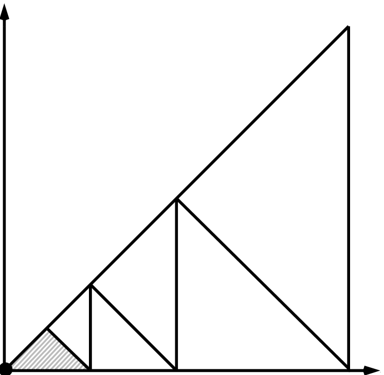
(a)

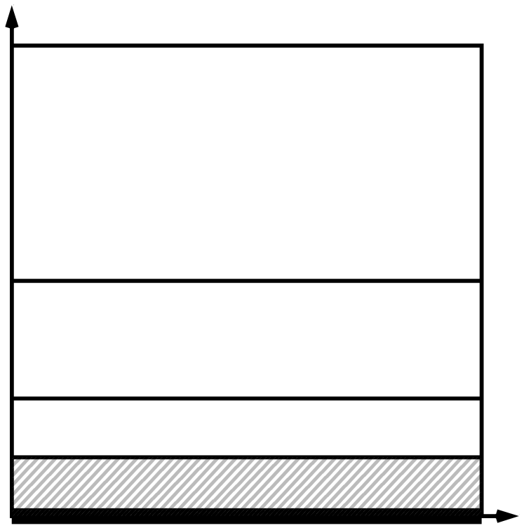
(b)

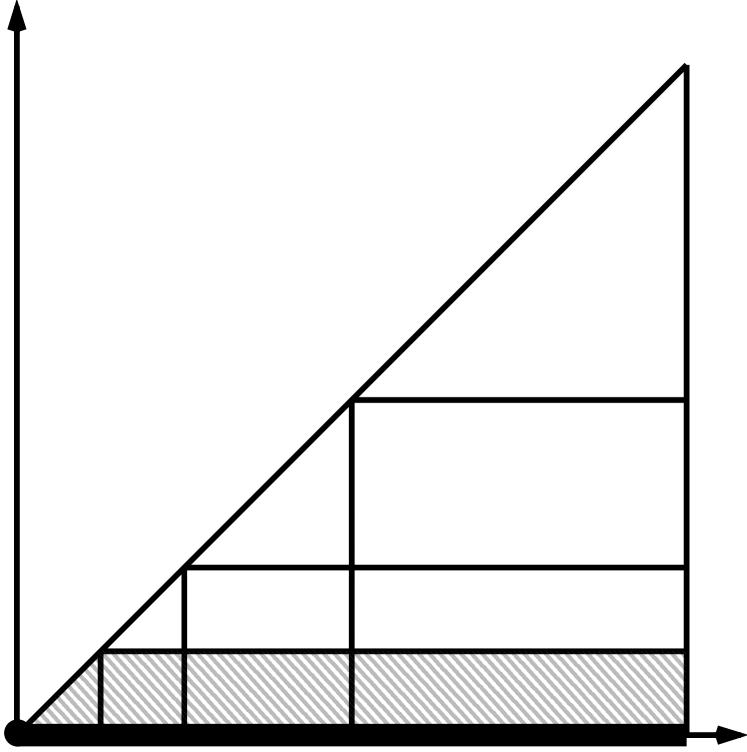
(c)

Figure 4: Boundary elements (displayed shaded) $\widetilde{\mathcal{L}}^{{\sf V},L}_{0}$, $\widetilde{\mathcal{L}}^{{\sf E},L}_{0}$, and $\widetilde{\mathcal{L}}^{{\sf VE},L}_{0}$ in the (4(a)) vertex, (4(b)) edge, and (4(c)) vertex-edge reference patches.

5.4.2 $hp$-FE approximation in reference vertex patch $\check{{\mathcal{T}}}^{{\sf V},L}_{\mathrm{geo},\sigma}$

We denote $\mathbf{v}=(0,0)$ and $\widetilde{r}_{\mathbf{v}}=\operatorname{dist}(\mathbf{v},\cdot)$. Furthermore, let

$$\widetilde{\mathcal{L}}^{{\sf V},L}_{0}=\{K\in\check{{\mathcal{T}}}^{{\sf V},L}_{\mathrm{geo},\sigma}:\overline{K}\cap\mathbf{v}\neq\emptyset\},\qquad\widetilde{T}^{{\sf V},L}_{\mathrm{int}}=\widehat{T}\setminus\bigcup_{K\in\widetilde{\mathcal{L}}^{{\sf V},L}_{0}}\overline{K},$$

be, respectively, the elements abutting the singular vertex and the interior part of the vertex reference patch, see Fig. 4(a).

Lemma 2 ($hp$-FE approximation in reference vertex patch $\check{{\mathcal{T}}}^{{\sf V},L}_{\mathrm{geo},\sigma}$)

For fixed $s\in(0,1)$ and $\gamma>0$, let $\widetilde{u}$ satisfy the following: for all $\varepsilon>0$ there exist a constant $C_{\varepsilon}>0$ such that for all $\alpha\in{\mathbb{N}}^{2}_{0}$ it holds, with $|\alpha|=p$, that

$$\left\|\tilde{r}_{\mathbf{v}}^{p-1/2-s+\varepsilon}\partial^{\alpha}\widetilde{u}\right\|_{L^{2}(\widehat{T})}\leq C_{\varepsilon}\gamma^{p+1}p^{p}.$$ (5.11)

Then, for all $\beta>1/2-s$ and all $0<\varepsilon<\beta+s-1/2$, there exist constants $b_{{\sf V}}>0$ (depending only on $\gamma$, $\beta$, $s$, $\sigma$) and $C_{{\sf V}}>0$ (depending additionally on $\varepsilon$) such that for every $L$, $q\in{\mathbb{N}}$

$$\|\widetilde{r}_{\mathbf{v}}^{\beta-1}(\widetilde{u}-\widetilde{\Pi}^{L}_{q}\widetilde{u})\|_{L^{2}(\widetilde{T}^{{\sf V},L}_{\mathrm{int}})}+\|\widetilde{r}_{\mathbf{v}}^{\beta}\nabla(\widetilde{u}-\widetilde{\Pi}^{L}_{q}\widetilde{u})\|_{L^{2}(\widetilde{T}^{{\sf V},L}_{\mathrm{int}})}\leq C_{{\sf V}}C_{\varepsilon}\exp(-b_{{\sf V}}q).$$ (5.12)

Proof

All elements ${\widetilde{K}}\in\check{{\mathcal{T}}}^{{\sf V},L}_{\mathrm{geo},\sigma}$ are shape regular: we denote by $h_{{\widetilde{K}}}$ their diameter. For all ${\widetilde{K}}\in\check{{\mathcal{T}}}^{{\sf V},L}_{\mathrm{geo},\sigma}\setminus\widetilde{\mathcal{L}}^{{\sf V},L}_{0}$, we have $\widetilde{r}_{\mathbf{v}}|_{{\widetilde{K}}}\simeq h_{{\widetilde{K}}}$ with equivalence constant uniform over $\check{{\mathcal{T}}}^{{\sf V},L}_{\mathrm{geo},\sigma}\setminus\widetilde{\mathcal{L}}^{{\sf V},L}_{0}$. From this equivalence and (5.11) it follows that, for all ${\widetilde{K}}\in\check{{\mathcal{T}}}^{{\sf V},L}_{\mathrm{geo},\sigma}\setminus\widetilde{\mathcal{L}}^{{\sf V},L}_{0}$ and all $\alpha\in\mathbb{N}^{2}_{0}$, there exists a constant $C_{1}>0$ such that

$$\left\|\widetilde{r}_{\mathbf{v}}^{|\alpha|}\partial^{\alpha}\widetilde{u}\right\|_{L^{2}({\widetilde{K}})}\leq C_{1}C_{\varepsilon}h_{{\widetilde{K}}}^{1/2+s-\varepsilon}\gamma^{|\alpha|+1}|\alpha|^{|\alpha|}.$$

By a scaling argument, then, there exists a constant $\gamma_{1}>0$ such that for all $\alpha\in\mathbb{N}^{2}_{0}$ and all ${\widetilde{K}}\in\check{{\mathcal{T}}}^{{\sf V},L}_{\mathrm{geo},\sigma}\setminus\widetilde{\mathcal{L}}^{{\sf V},L}_{0}$,

$$\left\|\widehat{\partial}^{\alpha}\left(\widetilde{u}\circ A^{L}_{{\widetilde{K}}}\right)\right\|_{L^{2}({\widehat{K}})}\leq C_{1}C_{\varepsilon}h_{{\widetilde{K}}}^{-1/2+s-\varepsilon}\gamma_{1}^{|\alpha|+1}\gamma^{|\alpha|+1}|\alpha|^{|\alpha|}$$

with ${\widehat{K}}=\widehat{T}=(A^{L}_{{{\widetilde{K}}}})^{-1}({\widetilde{K}})$. Recalling $\widehat{u}=\widetilde{u}\circ A^{L}_{{\widetilde{K}}}$, we can now exploit the embedding of $H^{2}({\widehat{K}})$ into $L^{\infty}({\widehat{K}})$ to obtain the existence of constants $C_{2},\gamma_{2}>0$ such that

$$\forall\alpha\in\mathbb{N}^{2}_{0}\colon\quad\|\widehat{\partial}^{\alpha}\widehat{u}\|_{L^{\infty}({\widehat{K}})}\leq C_{2}h_{{\widetilde{K}}}^{s-1/2-\varepsilon}\gamma_{2}^{|\alpha|+3}(|\alpha|+2)^{|\alpha|+2}.$$

It follows that there exists $C_{3}$, $\gamma_{3}>0$ such that

$$\forall{\widetilde{K}}\in\check{{\mathcal{T}}}^{{\sf V},L}_{\mathrm{geo},\sigma}\setminus\widetilde{\mathcal{L}}^{{\sf V},L}_{0}\quad\forall\alpha\in{\mathbb{N}}^{2}_{0}\colon\quad\|\widehat{\partial}^{\alpha}\widehat{u}\|_{L^{\infty}({\widehat{K}})}\leq C_{3}h_{{\widetilde{K}}}^{s-1/2-\varepsilon}\gamma_{3}^{|\alpha|+1}|\alpha|^{|\alpha|}.$$ (5.13)

From Lemma 5 and a scaling argument, it then follows that, for all $L,q\in{\mathbb{N}}$,

$$\|\widetilde{r}_{\mathbf{v}}^{\beta-1}(\widetilde{u}-\widetilde{\Pi}^{L}_{q}\widetilde{u})\|^{2}_{L^{2}({\widetilde{K}})}+\|\widetilde{r}_{\mathbf{v}}^{\beta}\nabla(\widetilde{u}-\widetilde{\Pi}^{L}_{q}\widetilde{u})\|^{2}_{L^{2}({\widetilde{K}})}\lesssim h_{{\widetilde{K}}}^{2\beta+{2}s-1-2\varepsilon}e^{-2bq}.$$

Since $\beta>1/2-s$, the power of $h_{{\widetilde{K}}}$ is non-negative for every $\varepsilon<\beta+s-1/2$ and summing the bound over all elements ${\widetilde{K}}\in\check{{\mathcal{T}}}^{{\sf V},L}_{\mathrm{geo},\sigma}\setminus\widetilde{\mathcal{L}}^{{\sf V},L}_{0}$ concludes the proof by a geometric series argument. ∎

5.4.3 $hp$-FE approximation in the reference edge patch $\check{{\mathcal{T}}}^{{\sf E},L}_{{\mathrm{geo}},\sigma}$

In this section, we denote $\mathbf{e}=\{y=0\}$ and $\widetilde{r}_{\mathbf{e}}=\operatorname{dist}(\mathbf{e},\cdot)$. Let $\widetilde{D}_{x_{\parallel}}=\partial_{x}$ and $\widetilde{D}_{x_{\perp}}=\partial_{y}$. Furthermore, let

$$\widetilde{\mathcal{L}}^{{\sf E},L}_{0}=\{K\in\check{{\mathcal{T}}}^{{\sf E},L}_{{\mathrm{geo}},\sigma}:\overline{K}\cap\mathbf{e}\neq\emptyset\},\qquad\widetilde{S}^{{\sf E},L}_{\mathrm{int}}=\widehat{S}\setminus\bigcup_{K\in\widetilde{\mathcal{L}}^{{\sf E},L}_{0}}\overline{K}$$

be, respectively, the elements abutting the singular boundary and the interior part of the edge reference patch, see Fig. 4(b).

Lemma 3 ($hp$-FE approximation in reference edge patch $\check{{\mathcal{T}}}^{{\sf E},L}_{{\mathrm{geo}},\sigma}$)

Let $s\in(0,1)$ and $\gamma>0$ be fixed, and let $\widetilde{u}$ be such that for all $\varepsilon>0$ there exists $C_{\varepsilon}>0$ such htat

$$\forall(p_{\perp},p_{\parallel})\in{\mathbb{N}}_{0}^{2}\colon\quad\left\|\tilde{r}_{\mathbf{e}}^{p_{\perp}-1/2-s+\varepsilon}\widetilde{D}^{p_{\perp}}_{x_{\perp}}\widetilde{D}^{p_{\parallel}}_{x_{\parallel}}\tilde{u}\right\|_{L^{2}(\widehat{S})}\leq C_{\varepsilon}\gamma^{p+1}p^{p},$$ (5.14)

with $p=p_{\perp}+p_{\parallel}$. Then, for all $\beta>1/2-s$ and all $0<\varepsilon<\beta+s-1/2$, there exist constants $b_{\sf E}>0$ (depending only on $\gamma$, $\beta$, $s$, $\sigma$) and $C_{{\sf E}}>0$ (depending additionally on $\varepsilon$) such that for every $L$, $q\in{\mathbb{N}}$

$$\|\widetilde{r}_{\mathbf{e}}^{\beta-1}(\tilde{u}-\widetilde{\Pi}^{L}_{q}\tilde{u})\|_{L^{2}(\widetilde{S}^{{\sf E},L}_{\mathrm{int}})}+\|\widetilde{r}_{\mathbf{e}}^{\beta}\nabla(\tilde{u}-\widetilde{\Pi}^{L}_{q}\tilde{u})\|_{L^{2}(\widetilde{S}^{{\sf E},L}_{\mathrm{int}})}\leq C_{{\sf E}}C_{\varepsilon}\exp(-b_{{\sf E}}q).$$ (5.15)

Proof

We denote by $h_{\parallel,{\widetilde{K}}}$ and $h_{\perp,{\widetilde{K}}}$ the edge-lengths of the rectangle ${\widetilde{K}}\in\check{{\mathcal{T}}}^{{\sf E},L}_{{\mathrm{geo}},\sigma}$ in, respectively, parallel and perpendicular directions to $\mathbf{e}$. For all ${\widetilde{K}}\in\check{{\mathcal{T}}}^{{\sf E},L}_{{\mathrm{geo}},\sigma}\setminus\widetilde{\mathcal{L}}^{{\sf E},L}_{0}$, we have $\widetilde{r}_{\mathbf{e}}|_{{\widetilde{K}}}\simeq h_{\perp,{\widetilde{K}}}$ with equivalence constant uniform over $\check{{\mathcal{T}}}^{{\sf E},L}_{{\mathrm{geo}},\sigma}\setminus\widetilde{\mathcal{L}}^{{\sf E},L}_{0}$. From (5.14), an anisotropic scaling argument, and a Sobolev embedding it follows that there exist $\widetilde{C},\widetilde{\gamma}>0$ such that

$$\forall{\widetilde{K}}\in\check{{\mathcal{T}}}^{{\sf E},L}_{{\mathrm{geo}},\sigma}\setminus\widetilde{\mathcal{L}}^{{\sf E},L}_{0},\,\forall(p_{\perp},p_{\parallel})\in{\mathbb{N}}_{0}^{2}:\qquad\|\widehat{\partial}^{(p_{\parallel},p_{\perp})}\widehat{u}\|_{L^{\infty}({\widehat{K}})}\leq\widetilde{C}h_{\perp,{\widetilde{K}}}^{s-\varepsilon}\widetilde{\gamma}^{p+1}p^{p}$$ (5.16)

with ${\widehat{K}}=\widehat{S}=(A^{L}_{{{\widetilde{K}}}})^{-1}({\widetilde{K}})$ and $p=p_{\parallel}+p_{\perp}$ (see the derivation of (5.13) for the detailed steps). From Lemma 6 and a scaling argument, it then follows that

$$\|\widetilde{r}_{\mathbf{e}}^{\beta-1}(\tilde{u}-\widetilde{\Pi}^{L}_{q}\tilde{u})\|^{2}_{L^{2}({\widetilde{K}})}+\|\widetilde{r}_{\mathbf{e}}^{\beta}\nabla(\tilde{u}-\widetilde{\Pi}^{L}_{q}\tilde{u})\|^{2}_{L^{2}({\widetilde{K}})}\lesssim h_{\perp,{\widetilde{K}}}^{2\beta+2s-1-2\varepsilon}e^{-2bq}.$$

Summing this bound over all ${\widetilde{K}}\in\check{{\mathcal{T}}}^{{\sf E},L}_{{\mathrm{geo}},\sigma}\setminus\widetilde{\mathcal{L}}^{{\sf E},L}_{0}$ using a geometric series argument concludes the proof since $\beta+s-1/2-\varepsilon>0$. ∎

5.4.4 $hp$-FE approximation in the reference vertex-edge patch $\check{{\mathcal{T}}}^{{\sf VE},L}_{{\mathrm{geo}},\sigma}$

In this section, we denote $\mathbf{v}=(0,0)$, $\mathbf{e}=\{y=0\}$, $\widetilde{r}_{\mathbf{v}}=\operatorname{dist}(\mathbf{v},\cdot)$, and $\widetilde{r}_{\mathbf{e}}=\operatorname{dist}(\mathbf{e},\cdot)$. Let $\widetilde{D}_{x_{\parallel}}=\partial_{x}$ and $\widetilde{D}_{x_{\perp}}=\partial_{y}$. Furthermore, let

$$\widetilde{\mathcal{L}}^{{\sf VE},L}_{0}=\{K\in\check{{\mathcal{T}}}^{{\sf VE},L}_{{\mathrm{geo}},\sigma}:\overline{K}\cap(\mathbf{e}\cup\mathbf{v})\neq\emptyset\},\qquad\widetilde{T}^{{\sf VE},L}_{\mathrm{int}}=\widehat{T}\setminus\bigcup_{K\in\widetilde{\mathcal{L}}^{{\sf VE},L}_{0}}\overline{K}$$

be, respectively, the elements abutting the singular boundary and the interior part of the vertex-edge reference patch, see Fig. 4(c).

Lemma 4 ($hp$-FE approximation in reference vertex-edge patch $\check{{\mathcal{T}}}^{{\sf VE},L}_{{\mathrm{geo}},\sigma}$)

Let $s\in(0,1)$ and $\gamma>0$ be fixed, and let $\widetilde{u}$ be such that for all $\varepsilon>0$ and there exists $C(\varepsilon)>0$ such that for all $(p_{\parallel},p_{\perp})\in{\mathbb{N}}_{0}^{2}$ with $p_{\parallel}+p_{\perp}=p$

$$\left\|\tilde{r}_{\mathbf{e}}^{p_{\perp}-1/2-s+\varepsilon}\widetilde{r}_{\mathbf{v}}^{p_{\parallel}+\varepsilon}\widetilde{D}^{p_{\perp}}_{x_{\perp}}\widetilde{D}^{p_{\parallel}}_{x_{\parallel}}u\right\|_{L^{2}(\widehat{T})}\leq C_{\varepsilon}\gamma^{p+1}p^{p}.$$ (5.17)

Then, for all $\beta>1/2-s$ and all $0<\varepsilon<\beta/2+s/2-1/4$, there exist constants $b_{\sf VE}>0$ (depending only on $\gamma$, $\beta$, $s$, $\sigma$) and $C_{{\sf VE}}>0$ (depending additionally on $\varepsilon$) such that for every $L$, $q\in{\mathbb{N}}$

$$\|\widetilde{r}_{\mathbf{e}}^{\beta-1}(\tilde{u}-\widetilde{\Pi}^{L}_{q}\tilde{u})\|_{L^{2}(\widetilde{T}^{{\sf VE},L}_{\mathrm{int}})}+\|\widetilde{r}_{\mathbf{e}}^{\beta}\nabla(\tilde{u}-\widetilde{\Pi}^{L}_{q}\tilde{u})\|_{L^{2}(\widetilde{T}^{{\sf VE},L}_{\mathrm{int}})}\leq C_{{\sf VE}}{C_{\varepsilon}}\exp(-b_{{\sf VE}}q).$$ (5.18)

Proof

Let ${\widetilde{K}}$ be an element not belonging to $\widetilde{\mathcal{L}}^{{\sf VE},L}_{0}$. We denote by $h_{\parallel,{\widetilde{K}}}$ and $h_{\perp,{\widetilde{K}}}$ the size of the rectangle ${\widetilde{K}}$ in, respectively, parallel and perpendicular directions to $\mathbf{e}$. We have $\widetilde{r}_{\mathbf{e}}|_{{\widetilde{K}}}\simeq h_{\perp,{\widetilde{K}}}$ and $\widetilde{r}_{\mathbf{v}}|_{{\widetilde{K}}}\simeq h_{\parallel,{\widetilde{K}}}$ with uniform equivalence constants. From (5.17), a scaling argument, and a Sobolev imbedding, it follows that there exist $\widetilde{C},\widetilde{\gamma}>0$ such that for all $(p_{\perp},p_{\parallel})\in{\mathbb{N}}_{0}^{2}$ with $p=p_{\parallel}+p_{\perp}$

$$\forall{\widetilde{K}}\in\check{{\mathcal{T}}}^{{\sf VE},L}_{{\mathrm{geo}},\sigma}\setminus\widetilde{\mathcal{L}}^{{\sf VE},L}_{0}\colon\quad\|\widehat{D}^{p_{\parallel}}_{x_{\parallel}}\widehat{D}^{p_{\perp}}_{x_{\perp}}\widehat{u}\|_{L^{\infty}({\widehat{K}})}\leq\widetilde{C}h_{\perp,{\widetilde{K}}}^{s-\varepsilon}h_{\parallel,{\widetilde{K}}}^{-1/2-\varepsilon}\widetilde{\gamma}^{p+1}p^{p}.$$ (5.19)

By a scaling argument (dropping temporarily the subscript $\cdot_{,{\widetilde{K}}}$)

$$\|\widetilde{r}_{\mathbf{e}}^{\beta-1}(\tilde{u}-\widetilde{\Pi}^{L}_{q}\tilde{u})\|^{2}_{L^{2}({\widetilde{K}})}+\|\widetilde{r}_{\mathbf{e}}^{\beta}\nabla(\tilde{u}-\widetilde{\Pi}^{L}_{q}\tilde{u})\|^{2}_{L^{2}({\widetilde{K}})}$$

$$\qquad\lesssim\begin{multlined}h_{\perp}^{2\beta}\bigg{(}\frac{h_{\parallel}}{h_{\perp}}\left(\|\widehat{u}-\widehat{\Pi}_{q}\widehat{u}\|^{2}_{L^{2}({\widehat{K}})}+\|\widehat{D}_{\perp}(\widehat{u}-\widehat{\Pi}_{q}\widehat{u})\|^{2}_{L^{2}({\widehat{K}})}\right)\\ +\frac{h_{\perp}}{h_{\parallel}}\|\widehat{D}_{\parallel}(\widehat{u}-\widehat{\Pi}_{q}\widehat{u})\|^{2}_{L^{2}({\widehat{K}})}\bigg{)}\end{multlined}h_{\perp}^{2\beta}\bigg{(}\frac{h_{\parallel}}{h_{\perp}}\left(\|\widehat{u}-\widehat{\Pi}_{q}\widehat{u}\|^{2}_{L^{2}({\widehat{K}})}+\|\widehat{D}_{\perp}(\widehat{u}-\widehat{\Pi}_{q}\widehat{u})\|^{2}_{L^{2}({\widehat{K}})}\right)\\ +\frac{h_{\perp}}{h_{\parallel}}\|\widehat{D}_{\parallel}(\widehat{u}-\widehat{\Pi}_{q}\widehat{u})\|^{2}_{L^{2}({\widehat{K}})}\bigg{)}$$

$$\qquad\leq h_{\perp}^{2\beta-1}h_{\parallel}\|\widehat{u}-\widehat{\Pi}_{q}\widehat{u}\|^{2}_{W^{1,\infty}({\widehat{K}})},$$

where the penultimate estimate follows from $h_{\perp}\simeq\widetilde{r}_{\mathbf{e}}\lesssim\widetilde{r}_{\mathbf{v}}\simeq h_{\parallel}$ in $\check{{\mathcal{T}}}^{{\sf VE},L}_{{\mathrm{geo}},\sigma}\backslash\widetilde{\mathcal{L}}^{{\sf VE},L}_{0}$. From Lemmas 5 and 6, using (5.19) then gives

$$\|\widetilde{r}_{\mathbf{e}}^{\beta-1}(\tilde{u}-\widetilde{\Pi}^{L}_{q}\tilde{u})\|^{2}_{L^{2}({\widetilde{K}})}+\|\widetilde{r}_{\mathbf{e}}^{\beta}\nabla(\tilde{u}-\widetilde{\Pi}^{L}_{q}\tilde{u})\|^{2}_{L^{2}({\widetilde{K}})}\lesssim h_{\perp,{\widetilde{K}}}^{2\beta+2s-1-2\varepsilon}h_{\parallel,{\widetilde{K}}}^{-2\varepsilon}e^{-2bq}.$$ (5.20)

From $\beta>1/2-s$ it follows that $\varepsilon>0$ can be chosen so that $2\beta+2s-1>4\varepsilon$. In addition, $h_{\perp,{\widetilde{K}}}\leq h_{\parallel,{\widetilde{K}}}$. Hence, there exists $\delta>0$ such that, for all $\varepsilon$ as specified above, $h_{\perp,{\widetilde{K}}}^{2\beta+2s-1-2\varepsilon}h_{\parallel,{\widetilde{K}}}^{-2\varepsilon}\leq h_{\perp,{\widetilde{K}}}^{\delta}$. Then,

$$\sum_{{\widetilde{K}}\in\check{{\mathcal{T}}}^{{\sf VE},L}_{{\mathrm{geo}},\sigma}\setminus\widetilde{\mathcal{L}}^{{\sf VE},L}_{0}}h_{\perp,{\widetilde{K}}}^{\delta} =(1-\sigma)^{\delta}\sum_{i=0}^{L-1}\sum_{j=i}^{L-1}\sigma^{\delta j}=\frac{(1-\sigma)^{\delta}}{1-\sigma^{\delta}}\sum_{i=0}^{L-1}\left(\sigma^{\delta i}-\sigma^{\delta L}\right)$$

$$\leq\frac{(1-\sigma)^{\delta}}{(1-\sigma^{\delta})^{2}}.$$

Summing (5.20) over all elements in $\check{{\mathcal{T}}}^{{\sf VE},L}_{{\mathrm{geo}},\sigma}\setminus\widetilde{\mathcal{L}}^{{\sf VE},L}_{0}$ concludes the proof. ∎

Remark 1

The dependence on $\varepsilon$ of the constants $C_{{\sf V}}$, $C_{{\sf E}}$, $C_{{\sf VE}}$ of Lemmas 2, 3, and 4 can be dropped if, for $\bullet\in\{{\sf V},{\sf E},{\sf VE}\}$, the constant $C_{\bullet}$ is replaced by $\widetilde{C}_{{\sf V}}L$ in (5.12), by $\widetilde{C}_{{\sf E}}L$ in (5.15), and by $\widetilde{C}_{{\sf VE}}L^{2}$ in (5.18). The newly introduced constants $\widetilde{C}_{\bullet}$ are independent of the choice of $\varepsilon$.

This has no effect on the final result. Considering the dependence of $C_{\bullet}$ on $\varepsilon$, a fixed value of $\varepsilon$ is chosen in the proof of Theorem 1.1, independently of $\beta$ and $s$. If one were to use instead the results with the constants $\widetilde{C}_{\bullet}$, the terms in $L$ and $L^{2}$ can be absorbed in the exponential $e^{-b_{\bullet}q}$ after having set $q\sim L$.  

5.4.5 Global error bound (Proof of Theorem 1.1)

Proof (Proof of Theorem 1.1)

Recall that $W^{L}_{q}=\mathcal{S}^{q}_{0}(\Omega,\mathcal{T}^{L}_{\mathrm{geo},\sigma})$ is the space of continuous, piecewise polynomials of maximum degree $q$ on a mesh with $L$ levels of refinement. From (5.9), Lemma 1, and Lemma 7 it follows that for all $\beta\in[0,1-s)$

$$\inf_{v\in W^{L}_{q}}\|u-v\|_{\widetilde{H}^{s}(\Omega)}\lesssim\|u-\Pi^{L}_{q-1}u\|_{H^{1}_{\beta}(\Omega\setminus\Omega^{L}_{0})}+\exp(-b_{1}L).$$ (5.21)

Remark that we can choose (potentially overlapping) $\omega_{\mathbf{v}}$, $\omega_{\mathbf{e}}$, and $\omega_{\mathbf{ve}}$ so that for all $K^{\mathcal{M}}\in\mathcal{T}^{\mathcal{M}}_{{\sf E}}$, $K^{\mathcal{M}}\subset\omega_{\mathbf{e}}$; for all $K^{\mathcal{M}}\in\mathcal{T}^{\mathcal{M}}_{{\sf VE}}$, $K^{\mathcal{M}}\subset\omega_{\mathbf{ve}}$; for all $K^{\mathcal{M}}\in\mathcal{T}^{\mathcal{M}}_{{\sf V}}$, either $K^{\mathcal{M}}\subset\omega_{\mathbf{v}}$ or $K^{\mathcal{M}}\subset\omega_{\mathbf{e}}$. In other words, the edge and vertex-edge patches in the domain $\Omega$ are, respectively, contained in $\omega_{\mathbf{e}}$ and $\omega_{\mathbf{ve}}$; the vertex patch is either contained in $\omega_{\mathbf{v}}$ or $\omega_{\mathbf{e}}$, with origin mapped to a point on a vertex or along an edge.

Suppose now that $u$ satisfies (2.5)–(2.8). Consider a patch $K^{\mathcal{M}}\in\mathcal{T}^{\mathcal{M}}$ and denote $\widetilde{u}=u\circ F_{K^{\mathcal{M}}}$. Let $\partial_{{\widetilde{x}}}$ be differentiation with respect to the variable ${\widetilde{x}}=F_{K^{\mathcal{M}}}^{-1}(x)$ and let $D_{{\widetilde{x}}_{\perp}}$ and $D_{{\widetilde{x}}_{\parallel}}$ be differentiation in directions respectively perpendicular and parallel to an edge pulled back to the reference patch. Let also $\widetilde{\mathbf{v}}=(0,0)$, $\widetilde{\mathbf{e}}=(0,1)\times\{0\}$ and denote $\widetilde{r}_{\mathbf{v}}({\widetilde{x}})=|{\widetilde{x}}-\widetilde{\mathbf{v}}|$, and $\widetilde{r}_{\mathbf{e}}({\widetilde{x}})=\operatorname{dist}({\widetilde{x}},\widetilde{\mathbf{e}})$, for all ${\widetilde{x}}\in F_{K^{\mathcal{M}}}^{-1}(K^{\mathcal{M}})$.

Case $K^{\mathcal{M}}\in\mathcal{T}^{\mathcal{M}}_{{\sf E}}$.

Since $F_{K^{\mathcal{M}}}$ is affine and since it maps the closure of $\{(x_{1},x_{2})\in\widehat{S}:x_{2}=0\}$ to $\partial\Omega\cap\partial K^{\mathcal{M}}$, its Jacobian $J_{F_{K^{\mathcal{M}}}}$ can be written as the composition of an upper triangular matrix $U_{K^{\mathcal{M}}}$ and a rotation $R_{K^{\mathcal{M}}}$:

$$J_{F_{K^{\mathcal{M}}}}=R_{K^{\mathcal{M}}}U_{K^{\mathcal{M}}}.$$

Without loss of generality, we may assume the coordinate systems oriented such that the vector $(1,0)^{\top}$, parallel to the singular edge in $\widehat{S}$, is mapped to $\mathbf{e}_{\parallel}=R_{K^{\mathcal{M}}}(1,0)^{\top}$. We remark that, since $U_{K^{\mathcal{M}}}$ is upper triangular, there exists $\eta_{K^{\mathcal{M}}}\in\mathbb{R}$ such that

$$U_{K^{\mathcal{M}}}(1,0)^{\top}=\eta_{K^{\mathcal{M}}}(1,0)^{\top}.$$

Hence,

$$D_{{\widetilde{x}}_{\parallel}}=\begin{pmatrix}1\\ 0\end{pmatrix}\cdot\nabla_{{\widetilde{x}}}=\begin{pmatrix}1\\ 0\end{pmatrix}\cdot(J_{F_{K^{\mathcal{M}}}}^{\top}\nabla_{x})=\eta_{K^{\mathcal{M}}}\begin{pmatrix}1\\ 0\end{pmatrix}\cdot(R_{K^{\mathcal{M}}}^{\top}\nabla_{x})=\eta_{K^{\mathcal{M}}}\mathbf{e}_{\parallel}\cdot\nabla_{x}=\eta_{K^{\mathcal{M}}}D_{x_{\parallel}}.$$

By a similar argument, there exist $\beta_{1},\beta_{2}\in\mathbb{R}$ such that

$$D_{{\widetilde{x}}_{\perp}}=\beta_{1}D_{x_{\parallel}}+\beta_{2}D_{x_{\perp}}.$$

Finally, there exists $c_{K_{M}}>0$ such that for all $x\in\widehat{S}$,

$$\frac{1}{c_{K^{\mathcal{M}}}}\widetilde{r}_{\mathbf{e}}(x)\leq r_{\mathbf{e}}(F_{K^{\mathcal{M}}}(x))\leq c_{K^{\mathcal{M}}}\widetilde{r}_{\mathbf{e}}(x).$$

Hence,

$$\left\|\tilde{r}_{\mathbf{e}}^{p_{\perp}-1/2-s+\varepsilon}D^{p_{\perp}}_{{\widetilde{x}}_{\perp}}D^{p_{\parallel}}_{{\widetilde{x}}_{\parallel}}\tilde{u}\right\|_{L^{2}(F_{K^{\mathcal{M}}}^{-1}(K^{\mathcal{M}}))}$$

$$\qquad\leq Cc_{K^{\mathcal{M}}}^{p_{\perp}-1/2-s+\varepsilon}\eta_{K^{\mathcal{M}}}^{p_{\parallel}}\|r_{\mathbf{e}}^{p_{\perp}-1/2-s+\varepsilon}(\beta_{1}D_{x_{\parallel}}+\beta_{2}D_{x_{\perp}})^{p_{\perp}}D_{x_{\parallel}}^{p_{\parallel}}u\|_{L^{2}(K^{\mathcal{M}})}$$

$$\qquad\leq Cc_{K^{\mathcal{M}}}^{p_{\perp}-1/2-s+\varepsilon}\eta_{K^{\mathcal{M}}}^{p_{\parallel}}(\beta_{1}+\beta_{2})^{p_{\perp}}\max_{j=0,\dots,p_{\perp}}\|r_{\mathbf{e}}^{p_{\perp}-1/2-s+\varepsilon}D_{x_{\perp}}^{j}D_{x_{\parallel}}^{p_{\parallel}+p_{\perp}-j}u\|_{L^{2}(K^{\mathcal{M}})}.$$

It follows then from (2.6) that there exist $\widetilde{C}_{\varepsilon},\widetilde{\gamma}>0$ such that, for all $(p_{\perp},p_{\parallel})\in{\mathbb{N}}_{0}^{2}$ with $p=p_{\perp}+p_{\parallel}$ and for all $K^{\mathcal{M}}\in\mathcal{T}^{\mathcal{M}}_{{\sf E}}$, we obtain

$$\left\|\tilde{r}_{\mathbf{e}}^{p_{\perp}-1/2-s+\varepsilon}D^{p_{\perp}}_{{\widetilde{x}}_{\perp}}D^{p_{\parallel}}_{{\widetilde{x}}_{\parallel}}\tilde{u}\right\|_{L^{2}(F_{K^{\mathcal{M}}}^{-1}(K^{\mathcal{M}}))}\leq\widetilde{C}_{\varepsilon}\widetilde{\gamma}^{p+1}p^{p}.$$

Case $K^{\mathcal{M}}\in\mathcal{T}^{\mathcal{M}}_{{\sf VE}}$.

This case is treated as the previous one, noting that in addition

$$\frac{1}{c_{K^{\mathcal{M}}}}\widetilde{r}_{\mathbf{v}}(x)\leq r_{\mathbf{v}}(F_{K^{\mathcal{M}}}(x))\leq c_{K^{\mathcal{M}}}\widetilde{r}_{\mathbf{v}}(x).$$ (5.22)

We obtain from (2.7) that there exist $\widetilde{C}_{\varepsilon},\widetilde{\gamma}>0$ such that, for all $(p_{\perp},p_{\parallel})\in{\mathbb{N}}_{0}^{2}$ with $p=p_{\perp}+p_{\parallel}$ and for all $K^{\mathcal{M}}\in\mathcal{T}^{\mathcal{M}}_{{\sf VE}}$,

$$\left\|\tilde{r}_{\mathbf{e}}^{p_{\perp}-1/2-s+\varepsilon}\widetilde{r}_{\mathbf{v}}^{p_{\parallel}+\varepsilon}D^{p_{\perp}}_{{\widetilde{x}}_{\perp}}D^{p_{\parallel}}_{{\widetilde{x}}_{\parallel}}\tilde{u}\right\|_{L^{2}(F_{K^{\mathcal{M}}}^{-1}(K^{\mathcal{M}}))}\leq\widetilde{C}_{\varepsilon}\widetilde{\gamma}^{p+1}p^{p}.$$

Case $K^{\mathcal{M}}\in\mathcal{T}^{\mathcal{M}}_{{\sf V}}$.

If $K^{\mathcal{M}}\subset\omega_{\mathbf{v}}$, then (5.22) holds. In addition, there exists a constant $\tilde{c}$ such that, for all $\alpha\in\mathbb{N}^{2}_{0}$,

$$\|\widetilde{r}_{\mathbf{v}}^{|\alpha|-1/2-s+\varepsilon}\partial_{{\widetilde{x}}}^{\alpha}\widetilde{u}\|_{L^{2}(F_{K^{\mathcal{M}}}^{-1}(K^{\mathcal{M}}))}\leq c_{K^{\mathcal{M}}}^{|\alpha|-1/2-s+\varepsilon}\tilde{c}^{|\alpha|}\max_{\beta\leq\alpha}\|r_{\mathbf{v}}^{|\alpha|-1/2-s+\varepsilon}\partial_{x}^{\beta}u\|_{L^{2}(K^{\mathcal{M}})}.$$ (5.23)

Therefore, (2.5) implies

$$\left\|\tilde{r}_{\mathbf{v}}^{|\alpha|-1/2-s+\varepsilon}\partial_{{\widetilde{x}}}^{\alpha}\tilde{u}\right\|_{L^{2}(F_{K^{\mathcal{M}}}^{-1}(K^{\mathcal{M}}))}\leq\widetilde{C}_{\varepsilon}\widetilde{\gamma}^{|\alpha|+1}|\alpha|^{|\alpha|}.$$

If instead $K^{\mathcal{M}}\subset\omega_{\mathbf{e}}$, there exists $c_{K^{\mathcal{M}}}$ such that

$$\frac{1}{c_{K^{\mathcal{M}}}}\widetilde{r}_{\mathbf{v}}(x)\leq r_{\mathbf{e}}(F_{K^{\mathcal{M}}}(x))\leq c_{K^{\mathcal{M}}}\widetilde{r}_{\mathbf{v}}(x)$$

for all $x\in K^{\mathcal{M}}$, with $\mathbf{e}$ being the edge such that $\mathbf{e}\cap\partial K^{\mathcal{M}}\neq\emptyset$. It follows from (5.23) and (2.6) that, for all $\alpha\in\mathbb{N}^{2}_{0}$,

$$\left\|\tilde{r}_{\mathbf{v}}^{|\alpha|-1/2-s+\varepsilon}\partial_{{\widetilde{x}}}^{\alpha}\tilde{u}\right\|_{L^{2}(F_{K^{\mathcal{M}}}^{-1}(K^{\mathcal{M}}))}\leq\widetilde{C}_{\varepsilon}\widetilde{\gamma}^{|\alpha|+1}|\alpha|^{|\alpha|}.$$

Case $K^{\mathcal{M}}\in\mathcal{T}^{\mathcal{M}}_{\mathrm{int}}$.

If $K^{\mathcal{M}}\in\mathcal{T}^{\mathcal{M}}_{\mathrm{int}}$, then $\widetilde{u}|_{F_{K^{\mathcal{M}}}^{-1}(K^{\mathcal{M}})}$ is analytic.

Since the macro triangulation $\mathcal{T}^{\mathcal{M}}$ is fixed, all constants depending on $K^{\mathcal{M}}$ can be taken uniformly over the macro triangulation. We have obtained that for all $K^{\mathcal{M}}\in\mathcal{T}^{\mathcal{M}}$, the restriction of $\widetilde{u}$ to $F^{-1}_{K^{\mathcal{M}}}(K^{\mathcal{M}})$ satisfies the hypotheses of Lemmas 2 to 4.

Restricting $\beta\in(1/2-s,1-s)$ in (5.21) and using Lemmas 2 to 4 gives therefore

$$\inf_{v\in W_{q}^{L}}\|u-v\|_{\widetilde{H}^{s}(\Omega)}\leq C\left(\exp(-b_{2}q)+\exp(-b_{1}L)\right).$$

Choosing $q\simeq L$, $V_{N}\coloneqq W^{L}_{q}$, and remarking that $\dim(W^{L}_{q})\simeq q^{2}L^{2}$ concludes the proof. ∎

6 Conclusions

We proved exponential rates of approximation for a class of $hp$-Finite Element approximations of the Dirichlet problem for the integral fractional Laplacian in a bounded, polygonal domain $\Omega\subset\mathbb{R}^{2}$, with analytic source term $f$, based on anisotropic, geometric boundary-refined meshes. The realization of corresponding $hp$-FE algorithms will incur significant issues of numerical quadrature for stable numerical evaluation of the bilinear form $a(\cdot,\cdot)$ in (1.5) on pairs of large aspect ratio rectangles in the geometric boundary mesh patches shown in Fig. 2. While being in princple known (see, e.g., SS97_317 for a related discussion in $hp$ Galerkin boundary element methods on polyhedral domains), the corresponding consistency analysis for the form $a(\cdot,\cdot)$ in (1.5) in the space $\widetilde{H}^{s}(\Omega)$ in (1.4) will be the topic of a forthcoming work.

Here, we analyzed only the convergence rate of the $hp$-Galerkin discretization (1.6) based on the subspaces $W^{L}_{q}$ in (5.1) with geometric, boundary-refined triangulations $\mathcal{T}^{L}_{\mathrm{geo},\sigma}$. Similar techniques, based again on the anisotropic, weighted high-order Sobolev regularity of the solution $u$ of (1.1) proved in FMMS21_983 , allow to infer optimal algebraic rates of convergence $O(h^{q+1-s})=O(N^{-(q+1-s)/2})$ in the $\widetilde{H}^{s}(\Omega)$-norm for continuous, piecewise polynomial Lagrangian Finite Elements of order $q\geq 1$. To this end, however, the geometric boundary-refined partitions $\mathcal{T}^{L}_{\mathrm{geo},\sigma}$ in the design of the spaces $W^{L}_{q}$ in (5.1) must be replaced by boundary-refined graded partitions. Details shall be reported elsewhere.

Appendix A Polynomial approximation operators on the reference element

The following two lemmas are consequences of (banjai-melenk-schwab19-RD, , Lemma 3.1, 3.2).

Lemma 5 (approximation on triangles)

Let $\widehat{T}$ be the reference triangle. Then, for every $q\in{\mathbb{N}}$, there exists a linear operator $\widehat{\Pi}^{\triangle}_{q}:C^{0}(\overline{\widehat{T}})\rightarrow{{\mathbb{P}}}_{q}$ with the following properties:

1. For each edge $e$ of $\widehat{T}$, $(\widehat{\Pi}^{\triangle}_{q}u)|_{e}$ coincides with the Gauss-Lobatto interpolant $i_{q}(u|_{e})$ of degree $q$ on the edge $e$.

2. (projection property) $\widehat{\Pi}^{\triangle}_{q}v=v$ for all $v\in{{\mathbb{P}}}_{q}$.

3. Let $u\in C^{\infty}(\widehat{T})$ satisfy, for some $C_{u}$, $\gamma>0$

   $$\forall n\in{\mathbb{N}}_{0}\colon\;\;\|\nabla^{n}u\|_{L^{\infty}(\widehat{T})}\leq C_{u}\gamma^{n}(n+1)^{n}.$$

   Then, there exist $C,b>0$ such that for all $q\geq 1$

   $$\|u-\widehat{\Pi}^{\triangle}_{q}u\|_{W^{1,\infty}(\widehat{T})}\leq CC_{u}e^{-bq}.$$

Lemma 6 (approximation on quadrilaterals)

Let $\widehat{S}$ be the reference square. For each $q\in{\mathbb{N}}$, the tensor-product Gauss-Lobatto interpolation operator $\widehat{\Pi}^{\Box}_{q}:C^{0}(\overline{\widehat{S}})\rightarrow{{\mathbb{Q}}}_{q}$ satisfies the following:

1. For each edge $e\subset\partial\widehat{S}$, $(\widehat{\Pi}^{\Box}_{q}u)|_{e}$ coincides with the univariate Gauss-Lobatto interpolant $i_{q}(u|_{e})$ on $e$.

2. (projection property) $\widehat{\Pi}^{\Box}_{q}v=v$ for all $v\in{{\mathbb{Q}}}_{q}$.

3. Let $u\in C^{\infty}(\widehat{S})$ satisfy for some $C_{u}$, $\gamma>0$, and all $(n,m)\in{\mathbb{N}}_{0}^{2}$

   $$\|\partial_{\widehat{x}}^{m}\partial_{\widehat{y}}^{n}u\|_{L^{\infty}(\widehat{S})}\leq C_{u}\gamma^{n+m}(n+1)^{n}(m+1)^{m}.$$ (A.1)

   Then, there exist $C,b>0$ such that for all $q\geq 1$

   $$\|u-\widehat{\Pi}^{\Box}_{q}u\|_{W^{1,\infty}(\widehat{S})}\leq CC_{u}e^{-bq}.$$

Appendix B Estimates of norms with cutoff function

We introduce two technical lemmas.

Lemma 7

Let $g^{L}$ be defined as in (5.7) and let $\beta\in[0,1)$. Then, there exists $C>0$ such that with $\Omega^{L}_{0}$ defined in (5.8), it holds, for all $w\in H^{1}_{\beta}(\Omega)$ and all $L\in\mathbb{N}$, that

$$\|g^{L}w\|_{H^{1}_{\beta}(\Omega)}\leq C\|w\|_{H^{1}_{\beta}(\Omega\setminus\Omega^{L}_{0})}.$$

Proof

By definition of $g^{L}$ we have for all $L\geq 1$

$$\|g^{L}\|_{L^{\infty}(\Omega)}=1,\qquad\|\nabla g^{L}\|_{L^{\infty}(\Omega)}\simeq\sigma^{-L}.$$

In addition, there exists $c>0$ such that for all $L\geq 1$

$$\operatorname*{supp}(\nabla g^{L})\subset S_{c\sigma^{L}}\setminus\Omega^{L}_{0},\qquad\operatorname*{supp}(1-g^{L})\subset S_{c\sigma^{L}},\qquad\operatorname*{supp}(g^{L})\subset\Omega\setminus\Omega_{0}^{L}.$$

Hence, for all $L\geq 1$,

$$\|r^{\beta-1}g^{L}w\|^{2}_{L^{2}(\Omega)}+\|r^{\beta}\nabla(g^{L}w)\|^{2}_{L^{2}(\Omega)}$$

$$\quad\leq\|r^{\beta-1}w\|^{2}_{L^{2}(\Omega\setminus\Omega_{0}^{L})}+\|\nabla g^{L}\|^{2}_{L^{\infty}(\Omega)}\|r^{\beta}w\|^{2}_{L^{2}(S_{c\sigma^{L}}\setminus\Omega_{0}^{L})}+\|r^{\beta}\nabla w\|^{2}_{L^{2}(\Omega\setminus\Omega_{0}^{L})}$$

$$\quad\lesssim\|w\|^{2}_{H^{1}_{\beta}(\Omega\setminus\Omega_{0}^{L})}+\sigma^{-2L}\|r^{\beta}w\|^{2}_{L^{2}(S_{c\sigma^{L}}\setminus\Omega_{0}^{L})}$$

$$\quad\lesssim\|w\|^{2}_{H^{1}_{\beta}(\Omega\setminus\Omega_{0}^{L})}+c^{2}\|r^{\beta-1}w\|^{2}_{L^{2}(S_{c\sigma^{L}}\setminus\Omega_{0}^{L})},$$

with constants hidden in $\lesssim$ independent of $L$. ∎

Lemma 8

Let $g^{L}$ be defined as in (5.7) and let $\beta\in[0,1)$. Then, there exist $C,c>0$ independent of $L$ such that, for all $w\in H^{1}_{\beta}(\Omega)$ and all $L\in\mathbb{N}$,

$$\|(1-g^{L})w\|_{H^{1}_{\beta}(\Omega)}\leq C\|w\|_{H^{1}_{\beta}(S_{c\sigma^{L}})}.$$

Proof

The proof proceeds along the same lines as the proof of the previous lemma. We have

$$\|r^{\beta-1}(1-g^{L})w\|_{L^{2}(\Omega)}\leq\|r^{\beta-1}w\|_{L^{2}(S_{c\sigma^{L}})},$$

where $c$ is defined as in the preceding proof such that $r(x)\leq c\sigma^{L}$ holds for all $x\in\operatorname*{supp}(1-g^{L})$. Similarly, we obtain

$$\|r^{\beta}\nabla((1-g^{L})w)\|^{2}_{L^{2}(\Omega)}\lesssim\|r^{\beta}\nabla w\|^{2}_{L^{2}(S_{c\sigma^{L}})}+c^{2}\|r^{\beta-1}w\|^{2}_{L^{2}(S_{c\sigma^{L}})},$$

which finishes the proof.∎

References

- [1] H. Abels and G. Grubb. Fractional-Order Operators on Nonsmooth Domains. arXiv e-prints, page arXiv:2004.10134, April 2020.
- [2] G. Acosta and J.P. Borthagaray. A fractional Laplace equation: regularity of solutions and finite element approximations. SIAM J. Numer. Anal., 55(2):472–495, 2017.
- [3] M. Ainsworth and C. Glusa. Aspects of an adaptive finite element method for the fractional Laplacian: a priori and a posteriori error estimates, efficient implementation and multigrid solver. Comput. Methods Appl. Mech. Engrg., 327:4–35, 2017.
- [4] L. Banjai, J.M. Melenk, R.H. Nochetto, E. Otárola, A.J. Salgado, and Ch. Schwab. Tensor FEM for spectral fractional diffusion. Found. Comput. Math., 19(4):901–962, 2019.
- [5] L. Banjai, J.M. Melenk, and Ch. Schwab. Exponential Convergence of -FEM for Spectral Fractional Diffusion in Polygons. Technical Report 2020-67, Seminar for Applied Mathematics, ETH Zürich, 2020.
- [6] L. Banjai, J.M. Melenk, and Ch. Schwab. -FEM for reaction-diffusion equations. II: Robust exponential convergence for multiple length scales in corner domains. Technical Report 2020-28, Seminar for Applied Mathematics, ETH Zürich, Switzerland, 2020.
- [7] A. Bonito, J.P. Borthagaray, R.H. Nochetto, E. Otárola, and A.J. Salgado. Numerical methods for fractional diffusion. Comput. Vis. Sci., 19(5-6):19–46, 2018.
- [8] A. Bonito, W. Lei, and J.E. Pasciak. Numerical approximation of the integral fractional Laplacian. Numer. Math., 142(2):235–278, 2019.
- [9] J.P. Borthagaray and R.H. Nochetto. Besov regularity for the Dirichlet integral fractional Laplacian in Lipschitz domains. arXiv e-prints, page arXiv:2110.02801, 2021.
- [10] J.P. Borthagaray and R.H. Nochetto. Constructive approximation on graded meshes for the integral fractional Laplacian. arXiv e-prints, 2021. arXiv:2109.00451.
- [11] L. Brasco and A. Salort. A note on homogeneous Sobolev spaces of fractional order. Ann. Mat. Pura Appl. (4), 198(4):1295–1330, 2019.
- [12] M. D’Elia, Q. Du, C. Glusa, M. Gunzburger, X. Tian, and Z. Zhou. Numerical methods for nonlocal and fractional models. Acta Numer., 29:1–124, 2020.
- [13] R.A. DeVore and G.G. Lorentz. Constructive Approximation. Springer Verlag, 1993.
- [14] M. Faustmann, M. Karkulik, and J.M. Melenk. Local convergence of the FEM for the integral fractional Laplacian. SIAM J. Numer. Anal., 60(3):1055–1082, 2022.
- [15] M. Faustmann, C. Marcati, J.M. Melenk, and Ch. Schwab. Weighted analytic regularity for the integral fractional Laplacian in polygons. Technical Report 2021-41, Seminar for Applied Mathematics, ETH Zürich, Switzerland, 2021. (to appear in SIAM Journ. Math. Analysis (2022).).
- [16] M. Faustmann, C. Marcati, J.M. Melenk, and Ch. Schwab. Exponential convergence of -FEM for the integral fractional Laplacian in 1d. Technical Report 2022-11, Seminar for Applied Mathematics, ETH Zürich, Switzerland, 2022.
- [17] M. Faustmann and J.M. Melenk. Robust exponential convergence of -FEM in balanced norms for singularly perturbed reaction-diffusion problems: corner domains. Comput. Math. Appl., 74(7):1576–1589, 2017.
- [18] H. Gimperlein, E.P. Stephan, and J. Štoček. Corner singularities for the fractional Laplacian and finite element approximation. preprint, 2021. http://www.macs.hw.ac.uk/hg94/corners.pdf.
- [19] P. Grisvard. Elliptic problems in nonsmooth domains, volume 69 of Classics in Applied Mathematics. Society for Industrial and Applied Mathematics (SIAM), Philadelphia, PA, 2011. Reprint of the 1985 original [ MR0775683], With a foreword by Susanne C. Brenner.
- [20] G. Grubb. Fractional Laplacians on domains, a development of Hörmander’s theory of -transmission pseudodifferential operators. Adv. Math., 268:478–528, 2015.
- [21] H. Holm, M. Maischak, and E. P. Stephan. Exponential convergence of the - version BEM for mixed boundary value problems on polyhedrons. Math. Methods Appl. Sci., 31(17):2069–2093, 2008.
- [22] M. Karkulik and J.M. Melenk. -matrix approximability of inverses of discretizations of the fractional Laplacian. Adv. Comput. Math., 45(5-6):2893–2919, 2019.
- [23] M. Kwaśnicki. Ten equivalent definitions of the fractional Laplace operator. Fract. Calc. Appl. Anal., 20(1):7–51, 2017.
- [24] A. Lischke, G. Pang, M. Gulian, F. Song, C. Glusa, X. Zheng, Z. Mao, W. Cai, M. M. Meerschaert, M. Ainsworth, and G. E. Karniadakis. What is the fractional Laplacian? A comparative review with new results. J. Comput. Phys., 404:109009, 62, 2020.
- [25] J.M. Melenk. -finite element methods for singular perturbations, volume 1796 of Lecture Notes in Mathematics. Springer-Verlag, Berlin, 2002.
- [26] R.H. Nochetto, E. Otárola, and A.J. Salgado. A PDE approach to fractional diffusion in general domains: a priori error analysis. Found. Comput. Math., 15(3):733–791, 2015.
- [27] X. Ros-Oton. Nonlocal elliptic equations in bounded domains: a survey. Publ. Mat., 60(1):3–26, 2016.
- [28] X. Ros-Oton and J. Serra. The Dirichlet problem for the fractional Laplacian: regularity up to the boundary. J. Math. Pures Appl. (9), 101(3):275–302, 2014.
- [29] S. Sauter and Ch. Schwab. Quadrature for -Galerkin BEM in . Numerische Mathematik, 78(2):211–258, 1997.
- [30] J. Štoček. Efficient finite element methods for the integral fractional Laplacian and applications. PhD thesis, Heriot-Watt University, 2020.
- [31] H. Triebel. Interpolation theory, function spaces, differential operators. Johann Ambrosius Barth, Heidelberg, second edition, 1995.