Microphase separation in neutral homopolymer blends induced by salt-doping

Abstract

Microphase separation in polymeric systems provides a bottom-up strategy to fabricate nanostructures. ^{1, 2, 3, 4} Polymers that are reported to undergo microphase separation usually include block copolymers or polyelectrolytes. Neutral homopolymers, which are comparatively easy to synthesize, are thought to be incapable of microphase separation. Here, using a minimal model that accounts for ion solvation, we show that microphase separation is possible in neutral homopolymer blends with sufficient dielectric contrast, upon a tiny amount of salt-doping. The driving force for the microphase separation is the competition between selective ion solvation, that places smaller ions in domains with higher dielectric constant, and the propensity for local charge neutrality to decrease the electrostatic energy. The compromise is an emergent length over which microphase separation occurs and ions are selectively solvated. The factors affecting such competitions are explored, including ion solvation radii, dielectric contrast, and polymer fraction, which point to directions for observing this behavior experimentally. These findings suggest a low-cost and facile alternative to produce microphase separation which may be exploited in advanced material design and preparation.

1 Background

Microphase separation results from the competition among multiple length-dependent interactions.⁵ A well-known example is block polymer, which is formed by chemically linking thermodynamically incompatible components.⁶ The incompatible blocks tend to separate from each other while the chemical linkages between blocks prevent macroscopic separation, giving rise to microphase separation.⁷ In the past, polymeric systems consisting of charged homopolymers (or polyelectrolytes, PE) are also shown to be capable of microphase separation. One example is weakly charged PEs in poor solvent. ^{8, 9, 10, 11, 12} The incompatibility between PE and solvent promotes a phase separation into two macroscopic phases with high and low PE concentrations. However, this leads to the loss in the translational entropy of counter ions, which mostly reside in the concentrated phase. The competition between the incompatibility-induced demixing and translational entropy loss of counter ions, leads finally to the microphase separation. Recently, it is suggested that microphase separation is also possible in polyelectrolytes blends, ^{13, 14} where the macroscopic phase separation between immiscible polyelectroytes is suppressed by the need to minimize coulombic interaction.

The analogy between the microphase separation of polyelectrolytes and diblock copolymer melts highlights the role of electrostatic interactions. Indeed, it has been found that electrostatic interaction can be leveraged to manipulate the phase behavior of polyelectrolytes solutions, ^{15, 16, 17} ionic polymer blends, ^{18, 19, 20} neutral diblock copolymer melts, ^{21, 22} or charged polymer blends ^{23, 24}. For example, selective solvation of doped salts in dielectrically heterogeneous copolymers has been shown to enhance the effective Flory-Huggins parameter between two blocks of diblock copolymer, ^{25, 26} favoring the formation of ordered microscopic phases. Remarkably, a “chimney” region was predicted where the solvation effects and electrostatic correlations of ions can promote microphase formation in an otherwise fully compatible diblock copolymer blends, that is, when the two blocks are fully miscible.²¹ Similarly in polyelectrolyte, counterions of PEs are predicted to be important in determining phase behavior, including enhancing the compatibility between two PEs, ^{27, 28} narrowing the parameter space for microphase separation, and allowing the competition between microphase and macrophase separation, etc. ²⁴

In this work, we show that selective ion solvation can be used not only to tune the microphase separation of neutral block copolymers or polyelectrolytes, but also to induce such transitions in neutral homopolymer blends. We develop a mean-field theory for salt-doped neutral homopolymer blends. The theory includes the Born solvation and electrostatic interactions of doping salt ions in addition to a free energy for neat homopolymer blends. ^{29, 22} A key feature of the theory is the heterogeneous dielectric constant, which depends on the local polymer fraction. With this theory, we find that under favorable conditions, the selective solvation of doped ions in domains with high dielectric constant causes a microscopic phase transition, in order to reduce the loss of translational entropy of ions.

2 Model and Theory

We consider binary blends of homopolymers A and B doped with salts. The degree of polymerization of the two polymers are $N_{\rm A}$ and $N_{\rm B}$. For simplicity, we only consider the case with one type of salt containing one cation species ($+$) and one anion species ($-$). The valencies of the cation and anion are $z_{+}$ and $z_{-}$, respectively. In a system containing $n_{\rm A}$ chains of polymer A, $n_{\rm B}$ chains of polymer B, $n_{+}$ cations, and $n_{-}$ anions, we can define the microscopic volume fraction $\hat{\phi}_{i}$ (and number density $\hat{\rho}_{i}$) of each component as,

$$\hat{\phi}_{\rm A}(\bf{r}) =v_{\rm A}\hat{\rho}_{\rm A}({\bf{r}})=v_{\rm A}\sum_{j=1}^{n_{\rm A}}\int_{0}^{N_{\rm A}}{\rm d}s\,\delta\left({\bf{r}}-{\bf{r}}_{j}^{\rm A}(s)\right),$$ (1)

$$\hat{\phi}_{\rm B}(\bf{r}) =v_{\rm B}\hat{\rho}_{\rm B}({\bf{r}})=v_{\rm B}\sum_{j=1}^{n_{\rm B}}\int_{0}^{N_{\rm B}}{\rm d}s\,\delta\left({\bf{r}}-{\bf{r}}_{j}^{\rm B}(s)\right),$$ (2)

$$\hat{\phi}_{\rm+}(\bf{r}) =v_{\rm+}\hat{\rho}_{\rm+}({\bf{r}})=v_{+}\sum_{j=1}^{n_{+}}\delta\left({\bf{r}}-{\bf{r}}_{j}^{+}\right),$$ (3)

$$\hat{\phi}_{\rm-}(\bf{r}) =v_{\rm-}\hat{\rho}_{\rm-}({\bf{r}})=v_{-}\sum_{j=1}^{n_{-}}\delta\left({\bf{r}}-{\bf{r}}_{j}^{-}\right).$$ (4)

Here, $v_{\alpha}$ with $\alpha\in\{{\rm A},{\rm B},+,-\}$ are the reference volume s for each component. The contour curves ${\bf{r}}_{j}^{p}(s)$, with $p\in\{{\rm A},{\rm B}\}$, represent the conformation of chain $j$, in which $s$ is the contour variable for monomers. By writing this, we treat the polymer as a continuous Gaussian chain. The positions of cation and anion are denoted as ${\bf{r}}_{j}^{+}$ and ${\bf{r}}_{j}^{-}$, respectively. The microscopic density is evaluated using the Dirac delta function $\delta(\bf{r})$, which is normalized and vanishes unless the argument equals $0$. In addition, the salt-doping level is conventionally quantified by the ratio between the number of cations and that of monomers of polymer with high dielectric constant, $r=n_{+}/(n_{\rm A}N_{\rm A})$.

To describe interaction in the blends, we use a minimal Hamiltonian that is capable of reproducing experimental phase diagrams of salt-doped diblock copolymer. ^{29, 30, 22} The Hamiltonian is composed of four terms and written explicitly as,

$$\beta\cal H= \beta({\cal H}^{\rm id}+U^{\rm FH}+U^{\rm B}+U^{\rm C})$$

$$= \sum_{j=1}^{n_{\rm A}}\int_{0}^{N_{\rm A}}\frac{3}{2b_{\rm A}^{2}}\left(\frac{{\rm d}{{\bf{r}}}_{j}^{\rm A}(s)}{{\rm d}s}\right)^{2}{\rm d}s$$

$$+\sum_{j=1}^{n_{\rm B}}\int_{0}^{N_{\rm B}}\frac{3}{2b_{\rm B}^{2}}\left(\frac{{\rm d}{{\bf{r}}}_{j}^{\rm B}(s)}{{\rm d}s}\right)^{2}{\rm d}s$$

$$+\frac{1}{v_{0}}\int{\rm d}{{\bf{r}}}\chi_{\rm AB}\hat{\phi}_{\rm A}({{\bf{r}}})\hat{\phi}_{\rm B}({{\bf{r}}})$$

$$+\int{\rm d}{{\bf{r}}}\frac{l_{0}}{2\hat{\epsilon}_{\rm r}(\bf{r})}\left(\frac{\hat{\phi}_{+}({{\bf{r}}})}{v_{+}a_{+}}+\frac{\hat{\phi}_{-}({{\bf{r}}})}{v_{-}a_{-}}\right)$$

$$+\frac{1}{2}\iint{\rm d}{{\bf{r}}}\,{\rm d}{{\bf{r}}}^{\prime}\,\hat{\rho}_{\rm q}({{\bf{r}}})g({{\bf{r}}},{{\bf{r}}}^{\prime})\hat{\rho}_{\rm q}({{\bf{r}}}^{\prime}).$$ (5)

Here, $\cal H^{\rm id}$ is the Hamiltonian of ideal Gaussian chains that accounts for the conformational statistics ³¹. $U^{\rm FH}$ is the Flory-Huggins interaction between two types of monomers, and $\chi_{\rm AB}$ is defined on a per-reference volume ($v_{0}$) basis.

The third term is for ion solvation. The interaction between ions and polymers is included in solvation free energy $U^{\rm B}$ approximated using the Born solvation model,³² and no dispersion interaction among ions is considered. The terms $l_{0}\equiv e^{2}/4\pi\epsilon_{0}k_{\rm B}T$, $v_{i}$, and $a_{i}$ are the vacuum Bjerrum length, ion volume, and ion diameter, respectively. The dielectric constant $\hat{\epsilon}_{\rm r}(\bf{r})$ is inhomogeneous and depends on the polymer composition at $\bf{r}$. In this work, we use a volumetric mixing rule for local dielectric constant, $\hat{\epsilon}_{\rm r}(\bf{r})=(\hat{\phi}_{\rm A}({{\bf{r}}})\epsilon_{\rm r,A}+\hat{\phi}_{\rm B}({{\bf{r}}}))\epsilon_{\rm r,B})/(\hat{\phi}_{\rm A}({{\bf{r}}})+\hat{\phi}_{\rm B}({{\bf{r}}}))$, where $\epsilon_{\rm r,A}$ and $\epsilon_{\rm r,B}$ are dielectric constant in pure homopolymer A and B. The ionic contributions to the dielectric constant are neglected, as we only consider situations with dilute salt contents.

The last term $U^{\rm C}$ is the Coulombic interaction of the net charge distribution, $\hat{\rho}_{\rm q}({\bf{r}})\equiv z_{+}\hat{\rho}_{+}({\bf{r}})+z_{-}\hat{\rho}_{-}({\bf{r}})=z_{+}\hat{\phi}_{+}({\bf{r}})/v_{+}+z_{-}\hat{\phi}_{-}({\bf{r}})/v_{-}$, in which $g({{\bf{r}}},{{\bf{r}}}^{\prime})$ is the Green’s function for Poisson’s equation with an inhomogeneous dielectric constant profile,

$$-\frac{1}{4\pi l_{0}}\nabla\cdot\epsilon_{\rm r}({\bf{r}})\nabla g({{\bf{r}}},{{\bf{r}}}^{\prime})=\delta^{3}({{\bf{r}}}-{{\bf{r}}}^{\prime}).$$ (6)

A key feature of our model related to Born and Coulomb terms is that the dielectric constant is inhomogeneous and depends on local polymer compositions $\phi_{\alpha}({\bf{r}})$, $\epsilon_{\rm r}({\bf{r}})=f[\phi_{\rm A}(\bf{r}),\phi_{\rm B}(\bf{r}))]$. As will become clear in the following, the selective ion solvation drives the microphase separation. It is therefore necessary to point out that the Born solvation free energy of an ion of species $\alpha$, $\sim 1/(a_{\alpha}\epsilon_{\rm r}({\bf{r}}))$, is inversely proportional to ion radius $a_{\alpha}$ and local dielectric constant $\epsilon_{\rm r}({\bf{r}})$. By this term alone, we may deduce that ions prefer to stay in domains with high dielectric constant and that the behavior of smaller ion is more susceptible to the solvation effects.

Following the standard field theory procedures, ^{7, 31, 22} which are detailed in Supplementary Information, we obtain the free energy as functionals of composition fields of all components, $\phi_{\alpha}({{\bf{r}}})$ with $\alpha~{}\in~{}\{\rm A,B,+,-\}$. In the disordered phase, the system is uniform and the composition fields are constant, $\phi_{\alpha}({{\bf{r}}})=\bar{\phi}_{\alpha}$. Therefore the free energy of the disordered phase can be written explicitly and we choose it as a reference state. For any composition fluctuations around the disordered phase, we can express the free energy change as Taylor expansion in terms of composition differences, ${\rm\delta}\phi_{\alpha}({{\bf{r}}})\equiv\phi_{\alpha}({{\bf{r}}})-\bar{\phi}_{\alpha}$. The expansion in Fourier space is written formally as,

$$\Delta{\cal F}= \ \Delta{\cal F}^{(2)}+\Delta{\cal F}^{(3)}+\Delta{\cal F}^{(4)}$$

$$= \ \frac{1}{2V^{2}}\sum_{{{\bf{q}}}}\sum_{\alpha,\beta}\Gamma^{(2)}_{\alpha\beta}({{\bf{q}}},-{{\bf{q}}})\delta\phi_{\alpha}({{\bf{q}}})\delta\phi_{\beta}(-{{\bf{q}}})$$ (7)

$$+\frac{1}{3!V^{3}}\!\sum_{{{\bf{q}}}_{1},{{\bf{q}}}_{2}}\sum_{\alpha,\beta,\gamma}\Gamma^{(3)}_{\alpha\beta\gamma}({{\bf{q}}}_{1},{{\bf{q}}}_{2},-{{\bf{q}}}_{1}-{{\bf{q}}}_{2})\delta\phi_{\alpha}({{\bf{q}}}_{1})\delta\phi_{\beta}({{\bf{q}}}_{2})\delta\phi_{\gamma}(-{{\bf{q}}}_{1}-{{\bf{q}}}_{2})+\cdots,$$

where $\alpha,\beta,\gamma,...$ denote species and ${{\bf{q}}}$ is wavevector. In our convention of Fourier transform, $f({{\bf{q}}})=\int{\rm d}{{\bf{r}}}f({{\bf{r}}})\exp(-{\rm i}{{\bf{q}}}\cdot{{\bf{r}}}).$ The vertex function, $\Gamma^{(n)}$, is $n$-th order functional derivatives of free energy change with respect to density deviations, evaluated at $\phi({{\bf{r}}})=\bar{\phi}$, or equivalently $\phi({{\bf{q}}})=\bar{\phi}\delta({{\bf{q}}})$.

The secondary expansion coefficient $\Gamma^{(2)}$ is a $4{\times}4$ matrix and its inverse is the structure factor measured in scattering experiments. It contains information about the nature of phase separation. Because of the isotropy of the homogeneous phase, the elements of $\Gamma^{(2)}$ are functions of $q=|{{\bf{q}}}|$, the wavenumber of density fluctuations. If we assume the blends are incompressible, the composition fluctuations should sum to zero, $\sum_{\alpha}\delta\phi_{\alpha}({{\bf{q}}})=0$. This means the composition fluctuation vector $\delta\phi=[\delta\phi_{\rm A},\delta\phi_{\rm B},\delta\phi_{\rm+},\delta\phi_{\rm-}]^{\rm T}$ is orthogonal to a compression mode ${\bf{\varepsilon}}=\frac{1}{2}[1,1,1,1]^{\rm T}$ and only exist in the orthogonal complement of the subspace of ${\bf{\varepsilon}}$. We therefore span the incompressible subspace by choosing an orthonormal basis set consisting of the following modes, ${\bf{e}}^{(1)}=\frac{1}{2}[1,1,-1,-1]^{\rm T}$, ${\bf{e}}^{(2)}=\frac{1}{2}[1,-1,1,-1]^{\rm T}$, and ${\bf{e}}^{(3)}=\frac{1}{2}[1,-1,-1,1]^{\rm T}$. After contracting the composition fluctuations to the incompressible subspace, we reduce the $4{\times}4$ matrix of $\Gamma^{(2)}(q)$ to a $3{\times}3$ matrix of $\gamma^{(2)}(q)$.

$\gamma^{(2)}(q)$ should have three eigenvalues $\lambda_{1}\leq\lambda_{2}\leq\lambda_{3}$. In the disordered phase, $\lambda_{1}(q)>0$, meaning that the free energy is concave up with respect to any composition fluctuation. The stability limit (i.e. the spinodal limit) of the disordered phase is given by the condition $\lambda_{1}(q^{*})=0$, where $q^{*}$ is a critical wavenumber that minimizes $\lambda_{1}$. The nature of the phase separation is indicated by the value of $q^{*}$. If $q^{*}>0$, the phase transition is microscopic and the ordered phase has a characteristic domain size of $D=2\pi/q^{*}$. If $q^{*}=0$, the characteristic domain size diverges and the phase separation is macroscopic.

3 Results and Discussions

3.1 Macrophase vs microphase separation

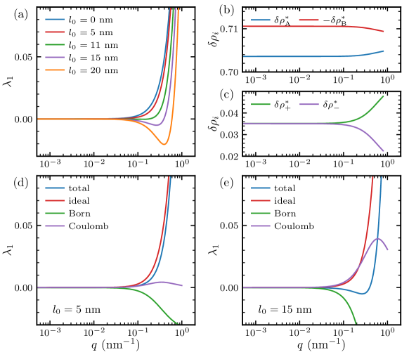
Figure 1: Spectral analysis of the quadratic vertex function of salt-doped homopolymer blends, with $\chi_{\rm AB}=0$ and $r=0.01$. (a) Minimum eigenvalue of quadratic coefficients ($\lambda_{1}$) as function of wavevector magnitude ($q$). The critical wavevector magnitude ($q^{*}$) corresponds to the location of the minimum of $\lambda_{1}$. The curves were shifted vertically so that the limit values at low $q$ were 0. (b) Polymeric components of eigenvector corresponding to $\lambda_{1}$, with $l_{0}=15.0\,{\rm nm}$. (c) Ionic components of eigenvector corresponding to $\lambda_{1}$, with $l_{0}=15.0\,{\rm nm}$. (d-e) Decomposition of $\lambda_{1}$ into contributions of ideal entropy, Born solvation, and Coulomb interaction for $l_{0}=5.0\,{\rm nm}$ (d) and $l_{0}=15.0\,{\rm nm}$ (e).

The competition between macroscopic and microscopic phase separation is governed by the strength of electrostatic interaction. We control the electrostatic contributions by tuning the vacuum Bjerrum length $l_{0}$. The Bjerrum length at room temperature is about 56 nm in vacuum and 0.7 nm in water. The (relative) dielectric constant for polymers is usually small, between 2 to 10, which corresponds to Bjerrum length of about 1.5 to 30 nm. A small Bjerrum length indicates strong electrostatic screening and weak electrostatic interactions.

We first consider a symmetric case with $v_{\rm A}=v_{\rm B}=v_{0}$ and $N_{\rm A}=N_{\rm B}=N$. Fig. 1a shows the minimum eigenvalue $\lambda_{1}$ of $\gamma^{(2)}$ versus $q$ for different Bjerrum lengths. When $l_{0}$ is small ($l_{0}=0{\text{ or }}5.0\,{\rm nm}$), $\lambda_{1}$ increases monotonically from $q=0$. The minimum of $\lambda_{1}(q)$ locates at $q^{*}=0$. Therefore only macrophase separation is possible in this regime. The limiting case of low electrostatic interaction is $l_{0}=0\,{\rm nm}$, where the electrostatic contribution to the free energy is essentially zero. This can also be seen from the expressions of the Born solvation energy, and Coulomb interaction energy (eq. 2). In this limit, the ions act as non-selective neutral solvents and it is well-known that only macroscopic separation can occur.

As the value of $l_{0}$ increases, $\lambda_{1}$ starts to change non-monotonically with $q$ (Fig. 1a). For $q<0.02\,{\rm nm}^{-1}$, $\lambda_{1}$ remains flat, resembling the cases with $l_{0}\leq 5\,{\rm nm}^{-1}$. However, beyond $q=0.02\,{\rm nm}^{-1}$, the value of $\lambda_{1}$ first decreases before finally increasing unboundedly. This non-monotonic behavior results in a finite critical wavevector $q^{*}>0$, signifying a microscopic phase separation. The value of $q^{*}$ increases and the non-monotonic shape becomes more pronounced as $l_{0}$ increases.

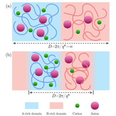
Figure 2: Schematic illustration of the competition between macrophase separation (a) and microphase separation (b).

To understand the nature of the instability at nonzero $q^{*}$, we examine the components of the critical mode, i.e., the eigenvector corresponding to the eigenvalue $\lambda_{1}$. The polymeric and ionic components of the critical modes are plotted in Fig. 1b and c, respectively. To evaluate the volume fractions for different components, we have used $\delta\phi^{*}=\sum_{i=1,2,3}\varphi_{i}^{*}{\bf{e}}^{(i)}$. The results shown in Fig. 1b are calculated from $\delta\phi^{*}$ by re-scaling each components with corresponding bead volume, i.e., $\delta\rho^{*}_{\alpha}=\delta\phi^{*}_{\alpha}/v_{i}$ for $\alpha\in\{{\rm A,B,+,-}\}$.

When $q$ is small ($q<0.02\,{\rm nm}^{-1}$), $\delta\rho^{*}_{\alpha}$ remain approximately constant. $\delta\rho^{*}_{\rm A}$ and $\delta\rho^{*}_{\rm B}$ have different signs as they tend to separate from each other. The amplitude $\delta\rho^{*}_{\rm A}$ is lower than $\delta\rho^{*}_{\rm B}$, which is compensated by the enrichment of ions in the A domain. The difference between cation and anion number density fluctuation mode ($\delta\rho_{\rm q}=\delta\rho^{*}_{+}-\delta\rho^{*}_{-}$) measures the degree of net charge separation. In the regime of $q<0.02\,{\rm nm}^{-1}$, $\delta\rho^{*}_{+}$ and $\delta\rho^{*}_{-}$ are essentially identical, implying the absence of charge separation. This is consistent with the expectation that charge separation at large length scale requires high energy cost.

In the high-$q$ regime, the magnitudes of $\delta\rho^{*}_{\rm A}$ and $\delta\rho^{*}_{+}$ increase, whereas those of $\delta\rho^{*}_{\rm B}$ and $\delta\rho^{*}_{-}$ decrease. This suggests that more cations are distributed in the A-rich domain while fewer anions reside in the A-rich domain. It is energetically favorable as the small diameter of cation affords a high (absolute value) Born solvation energy that overcompensates the loss of Born solvation energy from the anions that transferred to the B-rich domain. As $\delta\rho^{*}_{+}$ and $\delta\rho^{*}_{-}$ split, a net charge distribution also develops. The length scale at which charge separation begins to appear is about $\rm 60\,nm$, calculated from $2\pi/q^{*}$ by setting $q^{*}=0.1\,{\rm nm}^{-1}$, which is well within the range of Coulomb interaction.

To gain more insights into the origin of charge separation, we decompose $\lambda_{1}$ into contributions from the ideal, Born and Coulomb parts (Figs. 1d, e). The Flory-Huggins term is irrelevant because it is $q$-independent and we set $\chi_{\rm AB}=0$. All these terms remain constant in the small $q$ regime. The ideal part is similar for cases with $l_{0}=5\,{\rm nm}$ and $l_{0}=15\,{\rm nm}$. (Note that they are not identical, as their critical composition fluctuations differ slightly.) In the high-$q$ regime where charge separation takes place (Fig. 1c), we find that the decrease in the free energy is dominated by the decrease in the Born term (Figs. 1d,e). Furthermore, the Coulomb energy increases as the net charge developed. At even higher $q$ values, the Coulomb contributions decrease. This is because the total Coulomb energy decreases as the length scale of charge separation decreases.

The competition between the Born term and the ideal term contributes to the non-monotonic trend in $\lambda_{1}$ at large $q$ values. The value of $l_{0}$ controls the magnitude of Born and Coulomb terms. Only for sufficiently large $l_{0}$ values, can the Born solvation term dwarfs the ideal term that causes $\lambda_{1}$ to increase, resulting in a well-defined minimum.

The above discussions demonstrate that strong electrostatic interaction can trigger the microphase separation in homopolymer blends, as a result of the competition among multiple factors. The Born solvation promotes the localization of ions inside domains with higher dielectric permittivity, which drives phase separation so that the high permittivity domains can be formed. When this happens, both cations and anions tend to reside inside the high-permittivity phase, at the cost of the loss in translational entropy. One way to alleviate this frustration is to have smaller cations reside inside the high-permittivity domain, while allowing the anions to leak into the low-permittivity domains. However, this scenario implies macroscopic charge separation, which is energetically unfavorable: let the length scale for charge separation be $D$, then the magnitude of net charge $Q$ is proportional to $D$, and the Coulomb energy is of order $Q^{2}l_{0}/D\propto l_{0}D$, which blows up as $D\to\infty$. The compromise leads to the emergence of a finite domain size $D$, or $q^{*}$ value, when electrostatic interaction is sufficiently strong. The argument is illustrated in Fig. 2. The crossover from macrophase separation to microphase separation is identified as the Lifshitz point. ¹² The variation of the Lifshitz point and its dependence on model parameters are explored below.

3.2 Lifshitz point

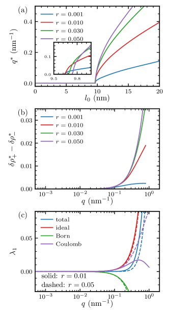
Figure 3: Dependence of critical $l_{0}$ on salt-doping amounts. (a) Critical wavevector magnitude ($q^{*}$) versus $l_{0}$ for different $r$ values. $q^{*}$ corresponds to the location of the minimum of $\lambda_{1}$ in Fig. 1a. (b) Salt-exchange degree as quantified by $\delta\rho^{*}_{+}-\delta\rho^{*}_{-}$ versus wavevector magnitude for different $r$ values. (c) Decomposition of $\lambda_{1}$ into contributions of ideal entropy, Born solvation, and Coulomb interaction for two $r$ values with $l_{0}=9.8\,{\rm nm}$.

When the dielectric ratio $\epsilon_{\rm A}/\epsilon_{\rm B}$ is fixed, the vacuum Bjerrum length $l_{0}$ is the primary factor determining the transition from macrophase to microphase separation. This is demonstrated in Fig. 3a, which shows how $l_{0}$ influences $q^{*}$, the wave number where the minimum of $\lambda_{1}$ locates (Fig. 1a), for different salt-doping levels $r$. The Lifshitz points, where $q^{*}$ first becomes nonzero, are located near $l_{0}=\rm 9.7nm$. With the range of salt doping levels explored, from 0.001 to 0.05, the location of Lifshitz point barely moves, as shown by the inset of Fig. 3a.

The weak dependence of the Lifshitz point on the doping level $r$ stems from the insensitivity of the degree of charge separation to $r$. Fig. 3b compares the degree of charge separation, quantified by the difference between the cationic and anionic components of the critical mode, for different doping levels. The results for different doping levels are nearly identical when $q<0.1\,{\rm nm^{-1}}$, which results in nearly identical contributions from the Born solvation term. In fact, for $q<0.1\,{\rm nm^{-1}}$, the contribution of the Born term to $\lambda_{1}$ are almost indistinguishable for $r=0.01$ and $r=0.05$ (Fig. 3c). This is precisely the range at which $q^{*}$ rises from 0 to finite values, which rationalizes why the location of the Lifshitz point is insensitive to the value of $r$.

The magnitude of $q^{*}$, i.e., the characteristic domain size, does depend on the doping level $r$ for $l_{0}>10\,{\rm nm}$. The higher the doping level, the greater the $q^{*}$ value, as seen from Fig. 3a. Such difference is also related to the progressively greater difference in the degree of charge separation for larger $q^{*}$ values, shown in Fig. 3b.

3.3 Spinodal curves

The above sections address the conditions for microphase separation. Here we examine the stability limit of the homogeneous phase, by evaluating the spinodal curves, which is found by requiring that $\lambda_{1}(q^{*})=0$. Here we recall that $\lambda_{1}$ is the minimum eigenvalue of the quadratic expansion coefficient $\gamma^{(2)}$ and $q^{*}$ is the critical wavevector that gives the minimum of $\lambda_{1}(q)$. The Flory-Huggins term, which was ignored in above sections by setting $\chi_{\rm AB}=0$, contributes $\delta\phi_{\rm A}\delta\phi_{\rm B}\chi_{\rm AB}$ to $\lambda_{1}$ for all $q$ ²², where $\delta\phi_{\alpha}$ is the $\alpha$-component of the eigenvector corresponding to $\lambda_{1}$. Therefore, changing $\chi_{\rm AB}$ effectively shifts the curves of $\lambda_{1}(q)$ vertically, and the spinodal can be readily found by requiring that the minimum of $\lambda_{1}(q)$ vanishes.

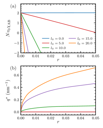
Figure 4: Spinodal behavior of salt-doped homopolymer blends. (a) Spinodal $\chi_{\rm AB}$ values versus doping degree ($r$) for different $l_{0}$ values. (b) Critical wavevector magnitude ($q^{*}$) versus $r$ for different $l_{0}$ values on the spinodal line.

The spinodal values of $\chi_{\rm AB}$ versus $r$, for several $l_{0}$ values, are plotted in Fig. 4a. All the spinodal curves converge to $Nv_{0}\chi_{\rm AB}=2.0$ at $r=0$, the well-known limit for symmetric binary homopolymer blends ³³. When $l_{0}=0\,{\rm nm}$, the ions became essentially non-selective solvents. The critical composition fluctuation is proportional to $[1,-1,0,0]^{\rm T}$ (data not shown), the same as neat symmetric homopolymer blends. The value of $\chi_{\rm AB}$ at the spinodal increases slightly with $r$, because of the dilution effects of non-selective solvents (the increment is minor for the range of $r$ is narrow). For nonzero $l_{0}$ values, the value of $\chi_{\rm AB}$ decreases with $r$, and the change is more substantial for larger $l_{0}$. This corroborates the notion that salt-doping can increase the effective $\chi$ parameter, as was first proposed by Wang ²⁵. However, Wang mainly considered the macrophase separation, whereas our focus is the emergence of microphase separation.

This point is highlighted by the critical wavenumber at the spinodal shown in Fig. 4b. Because the Flory-Huggins term does not alter the $q$-dependence of $\gamma_{2}$, the information contained in Fig. 4c is the same as that in Fig. 3b. Taken together, these results suggest that the crossover between macro- and micro-phase separation occurs slightly above $l_{0}=5\,\rm nm$.

3.4 Other factors

Using symmetric homopolymer blends as a model system, we have demonstrated the possibility of microphase separation upon salt-doping and studied the influence of salt content ($r$) and electrostatic interaction strength ($l_{0}$) in the above. In the following, we explore the influences of three key molecular properties: ion solvation radius, dielectric contrast, and polymer composition.

3.4.1 Ion solvation radius

The driving force for microphase separation in the system of interests is the need to simultaneously lower the Born solvation free energy, reduce the entropy loss of localized ions, and minimize the Coulomb energy. The Born solvation energy, eq. (2), is inverse to the ion solvation radius. Accordingly, we expect that the difference in ion solvation radii of cations and anions to be important. The parameterization for ion radii follows our recent study ³⁰, in which ionic volumes $v_{+}$ and $v_{-}$ are kept constant and ion radii $a_{+}$ and $a_{-}$ are varied.

Several combinations of ion solvation radii are explored, and the critical wavenumbers are plotted vs $l_{0}$ in Fig. 5a. The symmetric case with $a_{+}=a_{-}=0.1\,{\rm nm}$ is indifferent to the selective cation or anion solvation and charge separation cannot occur, so there is no microphase separation for all $l_{0}$ values. As $a_{-}$ increases, the discrepancy between cation and anion size grows, and the selective solvation of cations in the high-permittivity domain is stronger. We found that the value of $l_{0}$ at the Lifshitz point decreases from $\sim$20 nm to $\sim$7 nm as $a_{-}$ increases from $\rm 0.2\,nm$ to $\rm 0.8\,nm$, which supports our argument that a large difference between ion radii promotes microphase separation.

Additionally, when the solvation radii are doubled while the ratio $a_{+}/a_{-}$ is kept constant, the microphase separation is found to disappear. Doubling both ion solvation size act effectively halves the Born term. This reduction cannot be offset by simply doubling $l_{0}$, as doubling $l_{0}$ also increases energy cost from the Coulomb term, which weakens the energy gained from the Born term, making microphase separation impossible.

Fig. 5b presents the spinodal curves for different combinations of ion solvation radii. The trends of these curves are similar: the value of $\chi_{\rm AB}$ decreases as $l_{0}$ increases. There is, however, a weak increment when $l_{0}$ is small. This is the entropy regime of salt-doping, where adding ions stabilizes the homogeneous phase in order to achieve higher translational entropy ²². Because no microphase separation is expected in the entropy regime, we shall focus on the solvation regime below, where adding ions de-stabilizes the homogeneous phase. The decrease of $\chi_{\rm AB}$ with increasing $l_{0}$ depends only on the solvation size of ions and is insensitive to the ratio of the ion solvation radii. Smaller ions decreases $\chi_{\rm AB}$ more effectively, which is consistent with the findings of Nakamura et al. ²⁶. We note that such dependence is irrespective of the nature of phase separation, macroscopic or microscopic, consistent with the findings in Fig. 4.

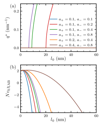
Figure 5: Effects of ionic solvation radii on the phase behavior of salt-doped homopolymer blends. Dependence of critical wavevector magnitude $q^{*}$ (a) and spinodal $\chi_{\rm AB}$ on $l_{0}$ (b) on $l_{0}$ for different combinations of ionic solvation radii ($a_{+}$ and $a_{-}$). Doping degree is $r=0.01$. The unit of ion solvation radius is nm.

3.4.2 Dielectric contrast

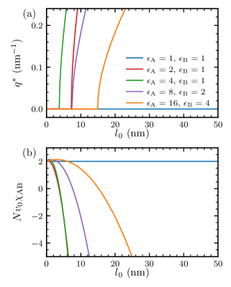
Figure 6: Effects of dielectric constant of polymer on the phase behavior of salt-doped homopolymer blends. Dependence of critical wavevector magnitude $q^{*}$ (a) and spinodal $\chi_{\rm AB}$ on $l_{0}$ (b) on $l_{0}$ for different combinations of polymer dielectric constant ($\epsilon_{\rm A}$ and $\epsilon_{\rm B}$). Doping degree is $r=0.01$.

The effects of dielectric contrast is analogous to that of the difference in ion solvation radii. The values of $q^{*}$ and the spinodal curves are shown in Fig. 6a, for different sets of dielectric permittivities. In the absence of dielectric contrast ($\epsilon_{\rm A}=\epsilon_{\rm B}=1$ in Fig. 6a), no microscopic separation is found. Because the net charge density vanishes, the ions act effectively as neutral solvents.

The microphase separation is possible with sufficient dielectric contrast. When we fix the dielectric constant of one polymer ($\epsilon_{\rm B}=1$), and increase $\epsilon_{\rm A}$ from 2 to 4, the value of $l_{0}$ at the Lifshitz point decreases from $\sim$7.5 nm to $\sim$3.7 nm (Fig. 6a). However, the spinodal $\chi_{\rm AB}$ does not change significantly from $\epsilon_{\rm A}=2$ to $\epsilon_{\rm B}=4$ (Fig. 6b). The quantitative dependence should be sensitive to the average rule chosen for the dielectric permittivity of mixtures²².

With a constant $\epsilon_{\rm A}/\epsilon_{\rm B}$, increasing both dielectric constants shifts the value of $l_{0}$ at the Lifshitz point to larger values. Both Born and Coulomb terms scale inversely with local dielectric constant. Doubling both dielectric constants reduces both terms by a factor of two. This is equivalent to reducing the Bjerrum length by a factor of two. As shown in Fig. 6a, when we change the dielectric constant from $(\epsilon_{\rm A},\epsilon_{\rm B})=(4,1)$ to $(8,2)$, the critical $l_{0}$ changes from $\sim$3.7 nm to $\sim$7.5 nm. Further change to $(16,4)$ gives a critical $l_{0}$ of $\sim$15.0 nm.

3.4.3 Polymer composition

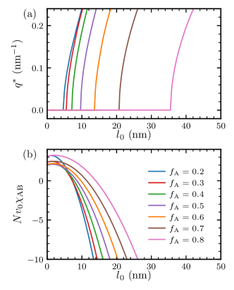
Figure 7: Effects of polymer fraction on the phase behavior of salt-doped homopolymer blends. Dependence of critical wavevector magnitude $q^{*}$ (a) and spinodal $\chi_{\rm AB}$ on $l_{0}$ (b) on $l_{0}$ for different fractions of A-polymer $f_{\rm A}$. Doping degree is $r=0.01$.

Fig. 7a shows that a higher fraction of high-permittivity component ($f_{\rm A}$) requires a larger $l_{0}$ to attain microphase separation. This is related to the translational entropy of ions. When macroscopic phase separation occurs, ions are distributed more preferably in the A-rich phase. A small $f_{\rm A}$ means the space available for ions is more restricted and hence a large loss of ionic translational entropy. The free energy gain is then more likely to drive a transition from macrophase separation to microphase separation.

A similar trend is found for how $f_{\rm A}$ affects the spinodal curves (Fig. 7b). When $l_{0}=0\,{\rm nm}$, spinodal $\chi_{\rm AB}$ values are the same as neat polymer blends, ³³ which is symmetric from $f_{\rm A}=0.5$. As $l_{0}$ increases, the value of $\chi_{\rm AB}$ at the spinodal decreases as expected but the changing rate is steeper for smaller $f_{\rm A}$ values. When $f_{\rm A}$ is large, the average dielectric constant in homogeneous phase is closer to $\epsilon_{\rm A}$, and the gain in the Born energy from ion localization is smaller, weakening the driving force for phase separation (either macroscopic or microscopic).

3.5 Why microphase separation induced by salt-doping seldom seen experimentally?

The region of microphase separation identified in our theory is rather broad (Fig. 4). However, such salt-doping-induced microphase separation in neutral homopolymer blends has not been reported. This may be attributed to the over-estimation of the solvation free energy by the simple Born expression. In reality, many factors can mitigate ion solvation free energy such as ion-paring, ion-clustering, and composition fluctuations ²². Other treatments of ion solvation such as dipolar SCFT, ^{34, 35, 36} liquid state theory corrected SCFT, ^{19, 21, 18} or classical density functional theory ^{37, 38, 39, 40} may help improve the accuracy of theoretical predictions but will not change our conclusions qualitatively. Formally weakening the Born solvation term implies that a higher $l_{0}$ value is required to induce microphase separation. To fulfill this condition, working with low-permittivity polymers is desirable. It remains to be seen, if tuning the ion solvation raii, dielectric contrast, and blending composition, as we explored above, can lead to experimental realization of microphase separation in doped polymer blends.

4 Conclusions

We developed a weak segregation theory for salt-doped neutral homopolymer blends. The model contains terms that describe the solvation free energy of ions and Coulombic interaction in addition to standard terms for neutral polymer blends, which has previously been used to analyze experimental phase diagrams ^{29, 30}. Our main result is that microphase separation may be induced when selective solvation is sufficiently strong.

The microphase separation permits local charge separation, with cations preferentially residing in the high-permittivity domains, whereas anions resides in the low-permittivity domains. The net result is that the Born solvation free energy is lower, ion entropy loss is reduced, and the Coulomb energy is minimal. The threshold value of $l_{0}$ at the crossover from the macro- to micro-phase separation is not sensitive to the amount of salt added. However, the doping level changes the critical $q^{*}$ significantly, which provides a facile means to tune the domain size of microphases.

We further probed how three key material properties, i.e., ion solvation radius, dielectric contrast, polymer fraction affect our results on microphase separation. It is found that larger solvation radius difference, larger dielectric contrast, and lower high-permittivity polymer composition, all favor the formation of microphases. Such observations may facilitate the experimental exploration of salt-induced microphase separation in polymer blends.

This work focused on the competition of microphase and macrophase separation and the stability limit of the homogeneous phase. The complete phase diagrams for salt-doped polymer blends, including the standard set of microphases (BCC, hexagonal, gyroid, etc.) ^{7, 29, 22} will be presented in the future.

This research has been supported by the Recruitment Program of Guangdong (grant no. 2016ZT06C322). J.Q. is supported by the National Science Foundation CAREER Award through DMR-1846547.

References

- Ouk Kim et al. 2003 Ouk Kim, S.; Solak, H. H.; Stoykovich, M. P.; Ferrier, N. J.; De Pablo, J. J.; Nealey, P. F. Epitaxial self-assembly of block copolymers on lithographically defined nanopatterned substrates. Nature 2003, 424, 411–414
- G. et al. 2012 G., A. T. K.; Gotrik, K. W.; Hannon, A. F.; Alexander-Katz, A.; Ross, C. A.; Berggren, K. K. Templating Three-Dimensional Self-Assembled Structures in Bilayer Block Copolymer Films. Science 2012, 336, 1294–1298
- Suh et al. 2017 Suh, H. S.; Kim, D. H.; Moni, P.; Xiong, S.; Ocola, L. E.; Zaluzec, N. J.; Gleason, K. K.; Nealey, P. F. Sub-10-nm patterning via directed self-assembly of block copolymer films with a vapour-phase deposited topcoat. Nature nanotechnology 2017, 12, 575–581
- Liu et al. 2018 Liu, C.-C.; Franke, E.; Mignot, Y.; Xie, R.; Yeung, C. W.; Zhang, J.; Chi, C.; Zhang, C.; Farrell, R.; Lai, K., et al. Directed self-assembly of block copolymers for 7 nanometre FinFET technology and beyond. Nature Electronics 2018, 1, 562–569
- Shi 2021 Shi, A.-C. Frustration in block copolymer assemblies. Journal of Physics: Condensed Matter 2021, 33, 253001
- Bates and Bates 2017 Bates, C. M.; Bates, F. S. 50th Anniversary Perspective: Block Polymers—Pure Potential. Macromolecules 2017, 50, 3–22
- Leibler 1980 Leibler, L. Theory of Microphase Separation in Block Copolymers. Macromolecules 1980, 13, 1602–1617
- Dormidontova et al. 1994 Dormidontova, E. E.; Erukhimovich, I.; Khokhlov, A. R. Microphase separation in poor‐solvent polyelectrolyte solutions: Phase diagram. Macromolecular Theory and Simulations 1994, 3, 661–675
- Borue and Erukhimovich 1988 Borue, V. Y.; Erukhimovich, I. Y. A statistical theory of weakly charged polyelectrolytes: fluctuations, equation of state and microphase separation. Macromolecules 1988, 21, 3240–3249
- Joanny, J.F. and Leibler, L. 1990 Joanny, J.F.,; Leibler, L., Weakly charged polyelectrolytes in a poor solvent. J. Phys. France 1990, 51, 545–557
- Gritsevich 2008 Gritsevich, A. V. Phase diagrams of polyelectrolyte solutions in poor solvents and of polyelectrolyte globules with allowance for microphase separation and fluctuation effects. Polymer Science Series A 2008, 50, 58–67
- Rumyantsev and Kramarenko 2017 Rumyantsev, A. M.; Kramarenko, E. Y. Two regions of microphase separation in ion-containing polymer solutions. Soft Matter 2017, 13, 6831–6844
- Rumyantsev and de Pablo 2020 Rumyantsev, A. M.; de Pablo, J. J. Microphase Separation in Polyelectrolyte Blends: Weak Segregation Theory and Relation to Nuclear “Pasta”. Macromolecules 2020, 53, 1281–1292
- Rumyantsev et al. 2019 Rumyantsev, A. M.; Gavrilov, A. A.; Kramarenko, E. Y. Electrostatically Stabilized Microphase Separation in Blends of Oppositely Charged Polyelectrolytes. Macromolecules 2019, 52, 7167–7174
- Sing and Perry 2020 Sing, C. E.; Perry, S. L. Recent progress in the science of complex coacervation. Soft Matter 2020, 16, 2885–2914
- Nakamura and Shi 2010 Nakamura, I.; Shi, A.-C. Self-consistent field theory of polymer-ionic molecule complexation. The Journal of Chemical Physics 2010, 132, 194103
- Nakamura 2016 Nakamura, I. Spinodal Decomposition of a Polymer and Ionic Liquid Mixture: Effects of Electrostatic Interactions and Hydrogen Bonds on Phase Instability. Macromolecules 2016, 49, 690–699
- Sing et al. 2013 Sing, C. E.; Zwanikken, J. W.; de la Cruz, M. O. Interfacial Behavior in Polyelectrolyte Blends: Hybrid Liquid-State Integral Equation and Self-Consistent Field Theory Study. Phys. Rev. Lett. 2013, 111, 168303
- Sing et al. 2013 Sing, C. E.; Zwanikken, J. W.; Olvera de la Cruz, M. Ion Correlation-Induced Phase Separation in Polyelectrolyte Blends. ACS Macro Letters 2013, 2, 1042–1046, PMID: 35581876
- Pryamitsyn et al. 2017 Pryamitsyn, V. A.; Kwon, H.-K.; Zwanikken, J. W.; Olvera de la Cruz, M. Anomalous Phase Behavior of Ionic Polymer Blends and Ionic Copolymers. Macromolecules 2017, 50, 5194–5207
- Sing et al. 2014 Sing, C. E.; Zwanikken, J. W.; Olvera de La Cruz, M. Electrostatic control of block copolymer morphology. Nature Materials 2014, 13, 694–698
- Kong et al. 2021 Kong, X.; Hou, K. J.-Y.; Qin, J. Weakening of Solvation-Induced Ordering by Composition Fluctuation in Salt-Doped Block Polymers. ACS Macro Letters 2021, 10, 545–550
- Grzetic et al. 2021 Grzetic, D. J.; Delaney, K. T.; Fredrickson, G. H. Electrostatic Manipulation of Phase Behavior in Immiscible Charged Polymer Blends. Macromolecules 2021, 54, 2604–2616
- Fredrickson et al. 0 Fredrickson, G. H.; Xie, S.; Edmund, J.; Le, M. L.; Sun, D.; Grzetic, D. J.; Vigil, D. L.; Delaney, K. T.; Chabinyc, M. L.; Segalman, R. A. Ionic Compatibilization of Polymers. ACS Polymers Au 0, 0, null
- Wang 2008 Wang, Z.-G. Effects of Ion Solvation on the Miscibility of Binary Polymer Blends. The Journal of Physical Chemistry B 2008, 112, 16205–16213, PMID: 19007274
- Nakamura et al. 2011 Nakamura, I.; Balsara, N. P.; Wang, Z.-G. Thermodynamics of Ion-Containing Polymer Blends and Block Copolymers. Phys. Rev. Lett. 2011, 107, 198301
- Zhang et al. 1990 Zhang, X.; Natansohn, A.; Eisenberg, A. Intermolecular cross-polarization studies of the miscibility enhancement of PS/PMMA blends through ionic interactions. Macromolecules 1990, 23, 412–416
- Zhang and Eisenberg 1990 Zhang, X.; Eisenberg, A. NMR and dynamic mechanical studies of miscibility enhancement via ionic interactions in polystyrene/poly (ethyl acrylate) blends. Journal of Polymer Science Part B: Polymer Physics 1990, 28, 1841–1857
- Hou and Qin 2018 Hou, K. J.; Qin, J. Solvation and Entropic Regimes in Ion-Containing Block Copolymers. Macromolecules 2018, 51, 7463–7475
- Hou et al. 2020 Hou, K. J.; Loo, W. S.; Balsara, N. P.; Qin, J. Comparing Experimental Phase Behavior of Ion-Doped Block Copolymers with Theoretical Predictions Based on Selective Ion Solvation. Macromolecules 2020, 53, 3956–3966
- Fredrickson 2013 Fredrickson, G. The Equilibrium Theory of Inhomogeneous Polymers; International Series of Monographs on Physics; OUP Oxford, 2013
- Wang 2010 Wang, Z.-G. Fluctuation in electrolyte solutions: The self energy. Phys. Rev. E 2010, 81, 021501
- de Gennes 1979 de Gennes, P. Scaling Concepts in Polymer Physics; Cornell University Press, 1979
- Nakamura 2014 Nakamura, I. Ion Solvation in Polymer Blends and Block Copolymer Melts: Effects of Chain Length and Connectivity on the Reorganization of Dipoles. The Journal of Physical Chemistry B 2014, 118, 5787–5796, PMID: 24806716
- Nakamura et al. 2012 Nakamura, I.; Shi, A.-C.; Wang, Z.-G. Ion Solvation in Liquid Mixtures: Effects of Solvent Reorganization. Phys. Rev. Lett. 2012, 109, 257802
- Nakamura 2015 Nakamura, I. Dipolar Self-Consistent Field Theory for Ionic Liquids: Effects of Dielectric Inhomogeneity in Ionic Liquids between Charged Plates. The Journal of Physical Chemistry C 2015, 119, 7086–7094
- Brown et al. 2018 Brown, J. R.; Seo, Y.; Hall, L. M. Ion correlation effects in salt-doped block copolymers. Phys. Rev. Lett. 2018, 120, 127801–1–127801–7
- Li and Wu 2006 Li, Z.; Wu, J. Density Functional Theory for Polyelectrolytes near Oppositely Charged Surfaces. Phys. Rev. Lett. 2006, 96, 048302
- Wu and Li 2007 Wu, J.; Li, Z. Density-Functional Theory for Complex Fluids. Annual Review of Physical Chemistry 2007, 58, 85–112, PMID: 17052165
- Kong et al. 2017 Kong, X.; Lu, D.; Wu, J.; Liu, Z. A theoretical study on the morphological phase diagram of supported lipid bilayers. Phys. Chem. Chem. Phys. 2017, 19, 16897–16903