Designing Autonomous Maxwell’s Demon via Stochastic Resetting

Abstract

Autonomous Maxwell’s demon is a new type of information engine proposed by Mandal and Jarzynski [Proc. Natl. Acad. Sci. U.S.A. 109, 11641 (2012)], which can produce work by exploiting an information tape. Here, we show that a stochastic resetting mechanism can be used to improve the performance of autonomous Maxwell’s demons notably. Generally, the performance is composed of two important features, the time cost for an autonomous demon to reach its functional state and its efficacious working region in its functional state. Here, we provide a set of design principles for the system, which are capable of improving the two important features. On the one hand, one can drive any autonomous demon system to its functional periodic steady state at a fastest pace for any initial distribution through resetting the demon for a predetermined critical time and closing the reset after that. On the other hand, the system can reach a new functional state when the resetting is always on, in which case the efficacious region of the demon could be extended significantly. Moreover, a dual-function region in a new phase diagram of the demon with resetting has been found. Remarkably, in this dual-function region the demon with resetting can realize anomalous output of work and erasure of information on the tape simultaneously, violating the second law of thermodynamics apparently. To this question, we derive a new modified Clausius inequality to restore the second law by taking the cost of resetting into account.

I Introduction

In 1867 Maxwell and Pesic (1871), James C. Maxwell conceived an intelligent creature to challenge the second law of thermodynamics, which usually refers to as “Maxwell’s demon” nowadays. The demon is capable of doing work only through harvesting information, which seems to violate the second law. This puzzle was finally clarified by Landauer and Bennet Landauer (1961); Bennett (1982). What the crucial point is that information needs to be stored in a physical memory, so that during each thermodynamic cycle an amount of energy should be cost to reset the memory, which promises the validity of second law. Maxwell’s thought experiment led to a series of interdisciplinary studies focusing on the interrelation between information theory and small-system thermodynamics. Recent years have witnessed great progress in this field named as information thermodynamics, including fruitful experimental works Rex (2017) and theoretical studies Parrondo et al. (2015).

Over the past 150 years, Maxwell’s-demon-like models have been subjected to extensive theoretical study Szilard (1929); Feynman et al. (2011); Mandal and Jarzynski (2012); Parrondo et al. (2015). Most of these models can be roughly divided into two classifications, one is measurement-feedback-controlled demon and another is autonomous demon. On the one hand, T. Sagawa and M. Ueda have developed the theoretical formalism of the first class of measurement-feedback demon Sagawa and Ueda (2012). On the other hand, Mandal and Jarzynski have constructed two analytically solvable autonomous demon models Mandal and Jarzynski (2012); Mandal et al. (2013), both consist of a memory-tape and a demon. These memory-tape autonomous demons can realize processes that are forbidden by the second law of thermodynamics by exploiting information. There are many subsequent works about these two kinds of Maxwell’s demon models Strasberg et al. (2014); Koski et al. (2015); Jurgens and Crutchfield (2020); Joseph and V. (2021); Debankur Bhattacharyya (2022); He et al. (2022); Sandberg et al. (2014); Manzano et al. (2021); Nahuel Freitas (2022). For instance, both of these two demon models are further generalized to quantum system Ryu et al. (2022); Deffner (2013); Poulsen et al. (2022).

Stochastic resetting, a rather common driving mechanism that stops a dynamical process randomly and starts it anew, has recently been of great interest in the field of statistical physics Evans and Majumdar (2011); Gupta et al. (2014); Reuveni (2016); Pal and Reuveni (2017); Belan (2018); Chechkin and Sokolov (2018); Pal et al. (2019); Miron and Reuveni (2021); De Bruyne et al. (2022, 2020). It has been shown that restarting a dynamical process stochastically may accelerate the process on average, which is counterintuitive. For instance, Evans and Majumdar Evans and Majumdar (2011) studied stochastic resetting theoretically for the first time,  claiming that the mean time for a freely diffusive Brownian particle to find a fixed target turns to be finite under constant rate Poisson resetting, while the mean time diverges without resetting. From then on, the resetting mechanism has been demonstrated to be advantageous to plenty of different stochastic processes such as animal foraging, RNA polymerases backtrack recovery Roldán et al. (2016) and relaxation processes Busiello et al. (2021). Furthermore, the effect of stochastic resetting on thermodynamics is also of interest Gupta et al. (2020); Busiello et al. (2020); Gupta and Busiello (2020); Pal et al. (2021); Fuchs et al. (2016); Pal and Rahav (2017). For more discussions of stochastic resetting see two recent reviews Evans et al. (2020); Gupta and Jayannavar (2022). Generally, this stochastic resetting mechanism could be used to optimize controlling protocols in small systems.

There are two important features of autonomous demons, which are main issues pertinent to the evaluation of their performances. The first feature is the relaxation time scale for the demon to reach its functional periodic steady state Cao et al. . It would be more accessible to initially prepare the demon in an equilibrium state which is generally not the periodic steady state, so there is some time cost for the demon to enter its working state and start transforming information resource into work. Certainly, the less time cost due to demon’s initial deviation from the functional state is more preferable. Another crucial feature is the demon’s efficacious working regions, including the region where positive work can be produced by exploiting information resources (information engine region) and the region in which the demon serve as a eraser that can replenish information resources (information eraser region, where the information entropy of the memory tape decreases on average). One would expect to extend those two working regions of the demon for better performance.

Here in the present work, we utilize the discrete-time stochastic resetting mechanism to provide designing principles of the autonomous Maxwell’s demon, improving demon’s performance in the two aspects of relaxation time-scale and efficacious working regions. To regulate those two main features of the autonomous demon, we introduce two kinds of resetting strategies leading to the reduction of time cost and the extension of the useful working regions respectively. The first type of strategy is to reset the demon to a given state with constant probability in discrete time (at the beginning of each cycle) for a fixed amount of time $t_{c}$, then turn off the reset and let the demon evolves according to the original dynamics. Strikingly, this can drive the demon to reach its functional periodic steady state at the fastest pace whatever its initial distribution is. This significant acceleration strategy is inspired by the so-called “strong” Mpemba effect, which recently received a lot of attention Gal and Raz (2020); Klich et al. (2019); Kumar and Bechhoefer (2020); Lu and Raz (2017); Santos and Prados (2020); Baity-Jesi et al. (2019). The second type of strategy is to keep resetting the demon to a given state, then the demon system will finally arrive at a new periodic steady state depending on the resetting rate. The new periodic steady state with resetting shows properties different to the original autonomous demon. In the phase diagram of this new autonomous demon with resetting, the information engine region is extended and the information eraser region is almost unchanged meanwhile. Remarkably, we find that there is an overlapping part of the information engine region and the information eraser region in the new phase diagram. We call this region the ’dual-function region’, where the second law of thermodynamics is apparently violated. To restore the second law, we derive a new Clausius inequality containing an extra term from the effect of stochastic resetting, which restores the second law of thermodynamics in the presence of resetting.

This article is organized as follows. In section II, we describe the methods to analyze autonomous Maxwell’s demon models introduced by Mandal and Jarzynski. Moreover, the formalism of discrete time stochastic resetting is introduced. In section III, we discuss the approach to induce significantly faster relaxations of the autonomous demon to functional periodic steady states via stochastic resetting strategy. New phase diagrams of an autonomous demon with the resetting mechanism always on is shown in section IV, where the anomalous work region is extended and the remarkably interesting ’dual-function’ region appears. In section V, we make some discussions and conclude the paper.

II Model and framework

Setup and analysis of the model

An autonomous Maxwell’s demon consists of a demon with $k$ states and an infinitely long memory tape (a stream of bits) encoding information with bit $0$ and $1$. In our setup, the $k$ - state demon is initially in equilibrium with a thermal reservoir at temperature $T_{\text{in}}$, then it would be coupled to a memory tape to constitute a $2k$ states combined system. This memory tape plays the roles of measurement and feedback as in the conventional Maxwell’s demon system. It moves through the demon at a constant speed to a given direction, with the bit sequence in the tape being written in advance (e.g. $0$11100…). The bit sequence is described by a probability distribution $\bm{p}_{\text{in}}^{B}=(p_{0},p_{1})^{\text{T}},$ where $p_{1}$ and $p_{0}$ are the probabilities of the incoming bit to be in states $1$ and $0$. For later use, we define $\delta\equiv p_{0}-p_{1}$ as the proportional excess of $0$’s among all incoming bits in the tape. The demon interacts with the incoming bits one by one as they pass by, i.e., it only interacts with the nearest bit for a fixed time $\tau$, after that the current bit leaves and a new bit comes in. During each interaction interval, there are intrinsic transitions between some pair of states of the demon. Moreover, the bit can transit between state $0$ and $1$ with the demon transiting between a state and another state meanwhile, and these type of cooperative transitions are not allowed to happen in the absence of either demon or bit. These cooperative transitions could bring about anomalous work production because the disordered transitions (just like fluctuations) of the $k$-state demon may be rectified by the incoming bits, which is the key idea of the autonomous demon. If the outgoing bit stream becomes more disordered than the incoming bit stream (the information entropy of the bit increase), then the transition of the demon is rectified to a given “direction” on average. The transition of demon to the given “direction” can produce work at the cost of information resources, while the opposite “direction” is useless. Which “direction” of transition can bring about positive work depends on the setup of the combined system. Throughout this paper, we set the bit transition from $0$ to $1$ as the right direction which can rectify the demon’s transitions , producing positive output work consequently.

Before proceeding, we list some notations for after use. Importantly, $t_{N}:=N\tau$ is the beginning time of the $N^{th}$ interaction interval, with $\tau$ being the interaction time of each interval. $\bm{p}^{D}(t)$ is a column vector with $k$ entries, which describes the probability distribution of the demon at time $t$. Similarly, $\bm{p}^{B}(t)$ is a vector with 2 entries, denoting the state of the bit at time $t$. $\bm{p}_{\tau}^{D}(t_{N})$ and $\bm{p}_{\tau}^{B}(t_{N})$ are the distributions of the demon and bit at the end of the $N^{th}$ interval, compared to $\bm{p}_{\text{in}}^{D}(t_{N})$ and $\bm{p}_{\text{in}}^{B}(t_{N})$ who are the distributions at the start of the $N^{th}$ interval. $\bm{p}(t)$ is the statistical state of the combined system with $2k$ entries. Finally, $\bm{p}_{\text{in}}^{D,ps}$, $\bm{p}_{\text{$\tau$}}^{D,ps}$and $\bm{p}_{\tau}^{B,ps}$ are the periodic steady state distributions at the beginning of intervals of the demon, and at the end of the intervals of the demon and the bit. The statistical state of the combined system comprised of the $k$ - state demon and the current bit (with two states $0$ or $1$) of the tape at the beginning time of the $N^{th}$ interval is given by the $2k$ dimensional vector

$$\bm{p}_{\text{in}}(t_{N})=\mathcal{M}\bm{p}_{\text{in}}^{D}(t_{N}),\ \ \text{$\mathcal{M}=$}\left(\begin{array}[]{c}p_{0}\mathbb{I}\\ p_{1}\mathbb{I}\end{array}\right),$$

where $\mathbb{I}$ is a $k\times k$ identity matrix and $\mathcal{M}$ is a $2k\times k$ matrix denoting a mapping from the demon subspace ($k\times 1$) to the total combined space ($2k\times 1$).What’s more, through defining some projectors, it would be also easy to extract the distributions in demon subspace and bit subspace from the distributions in the combined space at any time $t$, as follow:

$$\bm{p}^{D}(t) =\mathcal{P}^{D}\bm{p}(t),$$

$$\mathcal{P}^{D} =(\mathbb{I},\mathbb{I})$$ (1)

$$\bm{p}^{B}(t) =\mathcal{P}^{B}\bm{p}(t),$$

$$\mathcal{P}^{B} \equiv\left(\begin{array}[]{cccccc}1&...&1&0&...&0\\ 0&...&0&1&...&1\end{array}\right)_{2\times 2k},$$ (4)

with $\mathcal{P}^{D}$ and $\mathcal{P}^{B}$ denoting the projectors from the combined space to the demon subspace and to the bit subspace respectively. The combined system of the demon and the tape evolves under the master equation

$$\frac{d}{dt}\bm{p}(t)=\bm{R}\bm{p}(t)$$ (5)

during an interval from $t=N\tau$ to $t=(N+1)\tau$, where $\bm{R}$ is a $2k\times 2k$ transition matrix whose diagonal elements are $R_{ii}=-\sum_{i\neq j}R_{ji}$, and off-diagonal elements $R_{ji}$ are the transition rates from state $i$ to state $j$. As a result of the evolution equation (5), the probability distribution of the combined system at the end of the current interval reads $\bm{p}_{\tau}(t_{N})=e^{\bm{R}\tau}\bm{p}(t_{N})=\bm{e^{\bm{R}\tau}}\mathcal{M}\bm{p}^{D}(t_{N}).$ Then the corresponding statistical state of the demon can be written as

$$\bm{p}_{\text{in}}^{D}(t_{N+1})=\mathcal{T}\bm{p}_{\text{in}}^{D}(t_{N}),\ \ \mathcal{T}\equiv\mathcal{P}^{D}e^{\bm{R}\tau}\mathcal{M}$$

. According to the Perron-Frobenius theorem Meyer (2000), any initial distribution $\bm{p}_{\text{in},0}^{D}$ at the start of the first interval will evolve asymptotically to a unique periodic steady state

$$\bm{p}_{\text{in}}^{D,ps}=\lim_{n\rightarrow\infty}\mathcal{T}^{n}\bm{p}_{\text{\text{in},0}}^{D},$$ (6)

which can be obtained by solving the eigenvalue problem

$$\mathcal{T}\bm{p}_{\text{in}}^{D,ps}=\bm{p}_{\text{in}}^{D,ps}.$$ (7)

This unique periodic steady state is just the functional state of the autonomous Maxwell’s demon which can produce anomalous work stably. To calculate the work produced by the information engine through exploiting the memory tape, Mandal and Jarzynski have defined a quantity named as average production:

$$\Phi(\tau)\equiv p_{1}^{f}-p_{1}=p_{0}-p_{0}^{f},$$ (8)

where $p_{1}^{f}$ and $p_{0}^{f}$ are probabilities of the outgoing bit to be in states $1$ and $0$ (in the periodic steady state). The values of $p_{1}^{f}$ and $p_{0}^{f}$ are determined by

$$\bm{p}_{\tau}^{B,ps}\equiv\left(\begin{array}[]{c}p_{0}^{f}\\ p_{1}^{f}\end{array}\right)=\mathcal{P}^{B}e^{\bm{R}\tau}\mathcal{M}\bm{p}_{\text{in}}^{D,ps}.$$ (9)

then the average output work per interaction interval can be computed as (in the unit of $k_{B}T$)

$$\langle W\rangle=\Phi(\tau)\cdot w,$$

with $w$ being the work done by the combined system when a single jump of the bit from $0$ to $1$ happens. A positive value of $\langle W\rangle$ implies that the autonomous demon is converting information resources into work.

We take the simplest two-state demon model (named as information refrigerator) as an illustrative example, which is our main focus in this work. A demon with two energy states (up state $u$ with energy $E_{u}$ and down state $d$ with energy $E_{d}$) is coupled with a memory tape to comprise a four-state combined system (Fig. 1), with two heat baths at different temperatures being the environment. During each interaction interval, the combined system interacts with the heat bath at high temperature $T_{h}$ when the demon is jumping randomly between up state and down state by itself, with the current bit being unchanged. These intrinsic transitions of the demon is irrelevant to bits. Moreover, another kind of cooperative transitions $0d\leftrightarrow 1u$ are allowed , i.e., demon’s transitions from down state to up state shall only occur if the current bit makes a transition from $0$ to $1$ meanwhile, and from up state to down state only when the bit transit from $1$ to $0.$ These cooperative transitions happen in contact with the heat bath at low temperature $T_{c}$, being accompanied by exchanging energy with the cold heat bath. All transition rates of intrinsic transitions ($R_{d\rightarrow u},\ R_{u\rightarrow d}$) and cooperative transitions ($R_{0d\rightarrow 1u},\ R_{1u\rightarrow 0d}$) satisfy the detailed balance conditions as follow:

$$\text{$\frac{R_{d\to u}}{R_{u\to d}}=$}e^{-\beta_{h}\Delta E},\ \text{$\frac{R_{0d\to 1u}}{R_{1u\to 0d}}=$}e^{-\beta_{c}\Delta E}$$

where $\beta_{h,c}=1/(k_{B}T_{h,c})$. For later convenience, we parameterize them as : $R_{d\to u}=\Gamma(1-\sigma),R_{u\to d}=\Gamma(1+\sigma),\ R_{0d\to 1u}=1-\omega,R_{u\to d}=1+\omega$. The characteristic transition rate $\Gamma$ is set to be $1$ in the rest of the text. Here, $0<\sigma=\tanh\left(\beta_{h}\Delta E/2\right)<1$ and $0<\omega=\tanh\left(\beta_{c}\Delta E/2\right)<1$. We also define

$$\epsilon=\frac{\omega-\sigma}{1-\omega\sigma}=\tanh\frac{\left(\beta_{c}-\beta_{h}\right)\Delta E}{2},$$

with $0<\epsilon<1$ quantifying the temperature difference between the two reservoirs.

For each interaction interval, if a single bit turns from $0$ to $1$ due to the cooperative transition, then a fixed amount of energy $\Delta E=E_{u}-E_{d}$ is extracted from the cold reservoir, which can be identified as the anomalous work done by the demon. Consequently, the average output work due to the two-state demon in this model reads $\langle W\rangle\equiv Q_{c\rightarrow h}=\Phi(\tau)\cdot w=\Phi(\tau)(E_{u}-E_{d})$, where the average production $\Phi(\tau)$ can be computed using equations (3) - (5). More details about this model are described in the Appendix B.

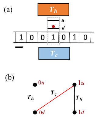
Figure 1: The information refrigerator model. (a) The two-state demon interacts with a sequence of bits and two reservoir at different temperature. (b) Graph depiction of the composite $4$-state system. Nodes denote the combined states and edges denote the allowed transitions, and each pair of transitions satisfies detailed balance conditions. The red edge represents the transition under the low temperature $T_{c}$, the other edges correspond to the transition at temperature $T_{h}$.

Formalism of discrete-time stochastic resetting

Here we would like to introduce a discrete-time resetting mechanism, which is randomly imposed on the $k$-state demon at the end of each interaction interval with a probability $\gamma=1-e^{-r\tau}$. Under this setting, larger the resetting rate $r$ and the time interval $\tau,$ more possible a resetting event will happen at the end of an interval. When a resetting event takes place, the demon would be taken to a given state $\vec{\Delta}$ instantaneously. This discrete-time resetting process may be realized as follow: resetting events happen according to a continuous-time Poisson process with rate $r_{0}$, and all events would only occur very near the end point of each interval, bringing the demon to the given resetting state $\vec{\Delta}$. Denoting $\delta t$ as the time window that resetting events can happen near the end of each interval, the probability that there is at least one such event is given by $\gamma=1-e^{-r_{0}\delta t}$. We assume that $\delta t\ll\tau$ and $\delta t\propto\tau$, and define a (modified) resetting rate $r:=r_{0}\delta t/\tau$. Then the effect of resetting events near the end of an interval is approximately equal to the effect of a single resetting event exactly at the end of the interval with probability $\gamma=1-e^{-r\tau}.$ $\bm{p}_{\text{in,0}}^{D}$ denotes the initial distribution of demon, which is prepared as an equilibrium state by letting the demon be in contact with a thermal reservoir whose temperature is $T_{\text{in}}$ . As mentioned above, in the absence of resetting, the evolution of the state of demon at the beginning of each interval can be described as

$$\bm{p}_{\text{in}}^{D}(t_{N})=\mathcal{T}^{N}\bm{p}_{\text{in,0}}^{D}.$$ (10)

With fixed-rate resetting events all happening at the end of interaction intervals, the demon’s evolution reads

$$\bm{p}_{\text{in}}^{D}(r,t_{N})=e^{-r\tau}\mathcal{T}\bm{p}_{\text{in}}^{D}(r,t_{N-1})+(1-e^{-r\tau})\vec{\Delta}.$$ (11)

Thus the demon’s initial distribution at time $t=N\tau$ is formally determined by

$$\bm{p}_{\text{in}}^{D}(r,t_{N})=e^{-rN\tau}\bm{p}_{\text{in}}^{D}(t_{N})+\left(1-e^{-r\tau}\right)\sum_{n=0}^{N-1}\left[e^{-rn\tau}\vec{\Delta}_{n\tau}\right],$$ (12)

where $\vec{\Delta}_{n\tau}\equiv\mathcal{T}^{n}\vec{\Delta}$ refers to the state $\vec{\Delta}$ evolves to after $n$ intervals. This is a renewal equation connecting the distribution at the beginning of each interval under discrete-time resetting with the distribution under the reset-free dynamics. On the right hand side of Eq. 12, the first term $e^{-rN\tau}\bm{p}_{\text{in}}^{D}(t_{N})$ accounts for the situation when there is no resetting events until time $t=N\tau$, the corresponding probability of which is $e^{-rN\tau}$. The $n^{th}$ term in the summation denotes the case in which the last restart happened at time $t=(N-n)\tau$, whose probability is $\left(1-e^{-r\tau}\right)e^{-rn\tau}$. The summation of the probabilities of all possible events mentioned above is

$$p_{\text{tot}} =e^{-rN\tau}+\left(1-e^{-r\tau}\right)\sum_{n=0}^{N-1}e^{-rn\tau}$$

$$=e^{-rN\tau}+1-e^{-rN\tau}=1,$$

satisfying the normalization condition. Note that when $\tau\rightarrow 0$, our renewal equation for discrete-time-resetting distribution reduces to the continuous time counterpart as in Busiello et al. (2021).:

$$\bm{p}^{D}(r,t)=e^{-rt}\bm{p}^{D}(t)+r\int_{0}^{t}dt^{\prime}e^{-rt^{\prime}}\vec{\Delta}_{t^{\prime}},$$ (13)

because when $\tau\rightarrow 0$, one has $\left(1-e^{-r\tau}\right)\rightarrow r\tau\equiv rdt^{\prime}$.

To obtain the whole dynamics with resetting, it would be helpful to utilize the spectral analysis method, solving the eigenvalues problem of the evolution matrix $\mathcal{T}$. The matrix $\mathcal{T}$ has right eigenvectors $\left\{\bm{R}_{i}\right\}$ and left eigenvectors $\left\{\bm{L}_{i}\right\}$ satisfy $\mathcal{T}\bm{R}_{i}=\lambda_{i}\bm{R}_{i}$ and $\bm{L}_{i}^{\text{T}}\mathcal{\mathcal{T}}=\lambda_{i}\bm{L}_{i}^{\text{T}}$, with $\lambda_{i}$ the eigenvalues, which are sorted as $1=\lambda_{1}>\left|\lambda_{2}\right|\geq\left|\lambda_{3}\right|\geq...$ (we assume that $\text{$\lambda$}_{2}$ is non-degenerate). Then according to completeness relation the initial state $\bm{p}_{\text{in},0}^{D}$ and resetting state $\vec{\Delta}$ can be expanded separately as

$$\begin{cases}\bm{p}_{\text{in,0}}^{D}&=\bm{p}_{\text{in}}^{D,ps}+\sum_{i\geq 2}a_{i}\bm{R}_{i},\\ \vec{\Delta}&=\bm{p}_{\text{in}}^{D,ps}+\sum_{i\geq 2}d_{i}\bm{R}_{i}\text{.}\end{cases}$$ (14)

where $a_{i}=\frac{\bm{L}_{i}^{\text{T}}\cdot\bm{p}_{\text{in,0}}^{D}}{\bm{L}_{i}^{\text{T}}\cdot\bm{R}_{i}}$ and $d_{i}=\frac{\bm{L}_{i}^{\text{T}}\cdot\vec{\Delta}}{\bm{L}_{i}^{\text{T}}\cdot\bm{R}_{i}}$ are coefficients. Thus the state of the demon at the beginning of the $N^{th}$ time interval can be written as

$$\bm{p}_{\text{in}}^{D}(t_{N})=\mathcal{T}^{N}\bm{p}_{\text{in,0}}^{D}\bm{=p}_{\text{in}}^{D,ps}+\sum_{i\geq 2}a_{i}\lambda_{i}^{n}\bm{R}_{i},$$ (15)

and

$$\vec{\Delta}_{n\tau}\equiv\mathcal{T}^{n}\vec{\Delta}=\bm{p}_{\text{in}}^{D,ps}+\sum_{i\geq 2}d_{i}\lambda_{i}^{n}\bm{R}_{i}\text{.}$$ (16)

One can identify the second term on the right hand side of Eq. (15) as a slowest decaying mode dominating the relaxation time scale, once the second coefficient $a_{2}$ is not equal to zero. In this case, the relaxation timescale is typically characterized by $\tau_{\text{rel}}=-1/\ln\left|\lambda_{2}\right|$.

Next, we gives some detailed descriptions of the two resetting strategies we would use to devise the autonomous demon. The first resetting strategy is randomly resetting the demon to the reset state and then switching off the resetting after a given time $t_{c}=N_{c}\tau$, causing the system to evolve according to the original dynamics without resetting. The whole dynamics of the first strategy can be formulated as

$$\bm{p}_{\text{in}}^{D}(r,t_{N})= \left[\gamma\mathcal{T}\bm{p}_{\text{in}}^{D}(r,t_{N-1})+(1-\gamma)\vec{\Delta}\right]\Theta(N_{c}-N)$$

$$+ \mathcal{T}\bm{p}_{\text{in}}^{D}(r,t_{N-1})\Theta(N-N_{c})\text{,}$$ (17)

where $\Theta$ is the Heaviside step function. The first strategy may used to eliminate the slowest decaying mode (making $a_{2}=0$) so that the demon would reach its functional state at a greatly faster pace. The second strategy is simply to keep the stochastic resetting mechanism always on so that the combined system will eventually reach a new periodic steady state, whose properties depend on the resetting rate $r$. For an illustration of the two resetting strategies, see Fig. 2.

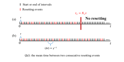
Figure 2: An illustration of two resetting strategies. (a) The first resetting strategy: closing the reset after a critical time $t_{c}$ (b) The second resetting strategy: always keeping the reset on.

Note that the resetting state is chosen to be a single state [e.g., $(0,1)^{\text{T}}$ for the two-state demon] instead of a mixed state in this work. Physically, resetting the demon to a mixture of distinct states effectively equals to resetting it to different single states randomly with different probabilities, which may be more technical for experimental realizations. Equipped with these discrete-time resetting formalism and the eigenvector-expansion formula, the designing principles for autonomous Maxwell’s demons are provided in the next two sections.

III Inducing Faster Relaxation

In this section, we show that how the first resetting strategy can accelerate the relaxation from an arbitrary initial distribution to demon’s functional steady state significantly. This significantly fast relaxation phenomenon induced by the stochastic resetting is similar to the Markovian Mpemba effect Lu and Raz (2017); Klich et al. (2019); Santos and Prados (2020); Baity-Jesi et al. (2019). We just turn off the resetting mechanism at a critical time $t_{c}=N_{c}\tau$, after which the demon system obeys the original evolutionary dynamics (10) with the coefficient of the relaxation mode ($i^{th}$ coefficient of the eigenvector expansion) $\bm{R}_{i}$ being $a_{i}(r,N_{c})$. Plugging (15) and (16) into equation (12) one can obtain (see Appendix A for details)

$$\bm{p}_{\text{\text{in}}}^{D}(r,t_{N})=\bm{p}_{\text{in}}^{D,ps}+\sum_{i\geq 2}a_{i}(r,N)\lambda_{i}^{N}\bm{R}_{i},$$ (18)

where the modified $i^{th}$ coefficient at $N^{th}$ interaction interval $a_{i}(r,N)$ reads

$$a_{i}(r,N)=\left[a_{i}-\frac{d_{i}\left(1-e^{-r\tau}\right)}{1-\lambda_{i}e^{-r\tau}}\right]e^{-rN\tau}+\frac{d_{i}\left(1-e^{-r\tau}\right)}{1-\lambda_{i}e^{-r\tau}}\cdot\lambda_{i}^{-N}.$$ (19)

Here $d_{i}$ is the $i^{th}$ coefficient of the expanded form of the $\vec{\Delta}$, depending on the choice of the reset state. Therefore, the whole dynamics under the first resetting strategy obeys

$$\begin{cases}\bm{p}_{\text{\text{in}}}^{D}(r,t_{N})=\bm{p}_{\text{in}}^{D,ps}+\sum_{i\geq 2}a_{i}(r,N)\lambda_{i}^{N}\bm{R}_{i}&N\leq N_{c}\\ \bm{p}_{\text{\text{in}}}^{D}(r,t_{N})=\bm{p}_{\text{in}}^{D,ps}+\sum_{i\geq 2}a_{i}(r,N_{c})\lambda_{i}^{N}\bm{R}_{i}&N>N_{c}\end{cases}.$$ (20)

By closing the reset at an appropriate critical time $t_{c}$, one can make the second coefficient being zero so that the relaxation gets significantly faster, corresponding to the so-called “strong” Mpemba effect. Combining $a_{2}(r,N)=0$ with Eq. (19) one gets the appropriate critical number of interaction intervals if the second eigenvalue $\lambda_{2}>0$ ($\lambda_{2}$ is demonstrated to be always positive in the models we study):

$$N_{c}=\frac{1}{r\tau-\ln\lambda_{2}}\ln\left[1-\frac{a_{2}}{d_{2}}\frac{1-\lambda_{2}e^{-r\tau}}{1-e^{-r\tau}}\right],$$ (21)

which is our first main result. From the expression of $N_{c}$ we clearly see that the condition for the existence of a physical critical number $N_{c}\geq 1$ is just $a_{2}/d_{2}\leq 0$. Furthermore, we are able to let $N_{c}$ be a small number like one through modifying the resetting rate $r$ whenever the condition $a_{2}/d_{2}\leq 0$ is fulfilled, thus the resetting strategy could always significantly reduce the total time cost to demon’s functional state compared to the reset-free dynamics. To show how this can be utilized to improve the performance of autonomous Maxwell’s demon, we focus on a specific model, the two-state information refrigerator mentioned above.

For the two-state information refrigerator, the resetting state could be $\vec{\Delta}_{d}=(0,1)^{\text{T}}$ or $\vec{\Delta}_{u}=(1,0)^{\text{T}}$, we choose the former one. Initially, we let the two-state demon be in contact with a heat bath whose temperature is $T_{\text{in}}$ for long enough time so that the demon reaches the thermal equilibrium. Then the initial distribution of the two-state demon is just

$$\bm{p}_{\text{in,0}}^{D}=\left(\frac{e^{-\Delta E/T_{\text{in}}}}{1+e^{-\Delta E/T_{\text{in}}}},\frac{1}{1+e^{-\Delta E/T_{\text{in}}}}\right)^{\text{T}},$$ (22)

which makes the second coefficient $a_{2}(T_{\text{in}})$ be a function of the initial temperature, so is the modified second coefficient $a_{2}(r,N,T_{\text{in}})$. It is clear from Eq. (21) that once the initial temperature allows the critical interaction number to be positive, then one can always make $N_{c}$ the smallest positive integer $1$ by virtue of adjusting the resetting constant $r$, whatever the dynamical details (i.e. values of $\delta=p_{0}-p_{1}$ and the temperature difference quantifier $\epsilon$ of the two heat baths) of the system is. Note that for the information refrigerator system, there is only one right eigenvector $\bm{R}_{2}$ as the relaxation mode, i.e.

$$\bm{p}^{D}(r,t_{N})=\bm{p}_{\text{in}}^{D,ps}+a_{2}(r,N,T_{\text{in}})\lambda_{2}^{N}\bm{R}_{2}.$$

In result, $a_{2}(r,N_{c},T_{\text{in}})=0$ signifies the arrival of the functional periodic steady state $\bm{p}_{\text{in}}^{D,ps}$. Thus for the two-state demon one can invariably expect the shortest time $t_{c}=\tau$ to enter the functional state through controlling the resetting parameter $r.$ In Fig. 3 we build a phase diagram for the dynamical behavior of the information engine before reaching its functional state. The blue area of the phase diagram corresponds to the fast relaxation ($a_{2}/d_{2}\leq 0$) region, where an optimal resetting rate that can lead to the smallest time cost $t_{c}=\tau$ always exists. This diagram provides guidance to prepare the initial state of the demon to be in an appropriate temperature. What’s more, if we set the up state as the reset state, the yellow area in the current diagram would turn to be the efficacious region of resetting. The asymmetry of the efficacious region corresponding to up state and down state arises from the energy difference between two states.

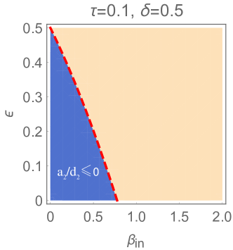
Figure 3: The phase diagram for the relaxation behavior of the information refrigerator. The parameter is set as $\tau=0.1,\$$\delta=0.5,$ $\Delta E=1$ and the reset state is the down state. The blue are is the fast relaxation region ($a_{2}/d_{2}\leq 0$), where the demon can reach the functional state significantly faster by stochastic resetting with appropriate rate. The yellow part is the dub region where resetting cannot take effect. However, if the reset state is set to be the up state, the yellow region would turn to be the useful region instead.

Then, to illustrate the accelerating effect of stochastic resetting, we further fix the dynamical parameters as $\delta=0.5,\ \epsilon=0.2$ and prepare the demon initially at $\beta_{\text{in}}=0.1$, then numerically gives several dynamical trajectories of the probability of the up state $p_{u}(t)$ under different resetting rates, as plotted in Fig. 4. Note that the resetting dynamics is switched off after a given critical time $t_{c}(r)=N_{c}(r)\tau$, depending on the resetting rate $r$. The optimal value of $r$ which can make $t_{c}=\tau$ is also a threshold value. It is shown in Fig. 4 that when the resetting rate $r$ is below this threshold value, the larger the $r$ is, the sooner the refrigerator could get to its functional periodic steady state. However, when the resetting rate is made to be larger than the optimal value, the time cost would become greater than $\tau.$ In the limiting case of $r\rightarrow\infty$, the demon would be reset to the down state (which can never be the functional state) with probability $1$ at the end of each interval, making the critical time $t_{c}$ go to zero, which is the same as the reset-free dynamics. In this given specific case, the threshold value of $r$ (or the optimal $r$) turns to be $1.82.$ To make it clearer, we plot the relation between the critical number $N_{c}$ and resetting rate $r$ in the inset of Fig.4, with the parameters being fixed at the same values as above.

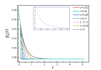
Figure 4: The evolution of the demon’s state under different resetting dynamics. For each dynamics with different resetting rate $r$, the resetting is closed right after the critical time $t_{c}(r)=N_{c}(r)\tau.$ We take the dynamics of probability of the up state as an illustration. The dynamical parameters are given by $\tau=0.1,\ \delta=0.5,\ \epsilon=0.2$ and $\beta_{\text{in}}=0.1$. The inset shows the relation between the critical number $N_{c}$ and the resetting rate $r$.

IV Autonomous Demon with Resetting

In this section, the second resetting strategy is taken into consideration, and the second features of the demon’s performance, i.e., the efficacious working region, is studied. To study the efficacious working region of demon, we first need to analyze the functional state performance of the autonomous demon with the second strategy being imposed on it. There are two crucial aspects of the functional state performance of the autonomous demon, including the average work production $\Phi$ per cycle and the information erasing capability quantified by the decrease of Shannon entropy of bit per cycle. If the autonomous demon is always under resetting, it will finally reach a new periodic steady state in the large time limit (the number of interactions $N\rightarrow\infty$), which is given by (see Appendix A for derivations)

$$\bm{p}_{\text{in}}^{D,ps}(r)=\bm{p}_{\text{in}}^{D,ps}+\sum_{i\geq 2}\frac{1-e^{-r\tau}}{1-\lambda_{i}e^{-r\tau}}d_{i}\bm{R}_{i}.$$ (23)

As a consequence, the marginal distribution of the outgoing bit in the new periodic steady state can be written as

$$\mathcal{P}_{\tau}^{B,ps}(r)=\mathcal{P}^{B}e^{\mathcal{R}\tau}\mathcal{M}\bm{p}_{\text{in}}^{D,ps}(r)=(p_{0}^{r},p_{1}^{r})^{\text{T}}.$$ (24)

Then, we would like to quantify the two important properties mentioned above in this new functional state, i.e., the average work production and the information erasing capability of the demon, so that the efficacious region could be analyzed in detail. Therefore, in the remaining part of this section, we assume the demon has reached its new functional periodic steady state. For simplicity, we take the two-state Maxwell’s refrigerator model as an illustrative example. The distribution of demon at the start of each interval is

$$\bm{p}_{\text{in}}^{D,ps}(r)=\bm{p}_{\text{in}}^{D,ps}+\frac{1-e^{-r\tau}}{1-\lambda_{2}e^{-r\tau}}d_{2}\bm{R}_{2}.$$

The performance of the information refrigerator with resetting can be evaluated by the average production of 1’s per interaction interval, recalling that the initial distribution of bit is given by $\bm{p}_{\text{\text{in}}}^{B}=(p_{0},p_{1})^{T}$:

$$\Phi_{\text{tot}}(r,\tau)\equiv p_{1}^{r}-p_{1}=p_{0}-p_{0}^{r}.$$ (25)

The average transfer of energy from the cold to the hot reservoir is $Q_{c\rightarrow h}=\Phi_{r}\Delta E=\Phi_{r}(E_{u}-E_{d}).$ The total average production per interaction interval is given by

$$\Phi_{\text{tot}} =\left(\left[\mathcal{T}^{{}^{\prime}}\bm{p}_{\text{in}}^{D,ps}\right]_{2}-p_{1}\right)+\frac{1-e^{-r\tau}}{1-\lambda_{2}e^{-r\tau}}d_{2}\left[\mathcal{T}^{{}^{\prime}}\bm{R}_{2}\right]_{2},$$

$$\equiv\Phi_{0}+\Phi_{r}$$ (26)

where $\mathcal{T}^{{}^{\prime}}=\mathcal{P}^{B}e^{\mathcal{R}\tau}\mathcal{M}$. It has been shown that (see Appendix B for details)

$$\Phi\equiv\left[\mathcal{T}^{{}^{\prime}}\bm{p}_{\text{in}}^{D,ps}\right]_{2}-p_{1}=\frac{\delta-\epsilon}{2}\eta(\Lambda),$$ (27)

thus we just need to compute the contribution $\Phi_{r}$ arising from stochastic reset. The second right eigenvector is obtained as $\bm{R}_{2}=(1,-1)^{T}$. We set the resetting state as $\vec{\Delta}=(0,1)^{T}$(down state) or $\vec{\Delta}=(1,0)^{T}$ (up state), and study their contributions respectively. When the demon is reset to the up state, we find that the contribution $\Phi_{r}$ always takes negative value whatever the value of $r$ is. This implies that the up state is not a good choice for the reset state because resetting the demon to up state only has negative impact on the engine’s performance, i.e., shrinking the refrigerator region. We will see that the down state $\vec{\Delta}=(0,1)^{T}$ would be an appropriate option for the demon to be reset to, even might be optimal.

Now consider another important feature of performance of the refrigerator in the new functional state, the information-processing capability of the demon. To quantify the capability, the Shannon entropy difference between the outgoing be and the incoming bit is introduced as

$$\Delta S_{B}= S(\bm{p}_{\text{$\tau$}}^{B,ps})-S(\bm{p}^{B,ps})=S(\delta-2\Phi_{\text{tot}})-S(\delta),$$

$$S(\delta)\equiv -\sum_{i=1}^{1}p_{i}\ln p_{i}$$

$$= -\frac{1-\delta}{2}\ln\frac{1-\delta}{2}-\frac{1+\delta}{2}\ln\frac{1+\delta}{2},$$ (28)

which is a measure of how much information content contained in the memory tape is changed due to the demon during each interaction interval.

At the end of the day, to illustrate the extended efficacious region of the refrigerator, we fix $\Gamma=1,\ \omega=1/2$ and construct a phase diagram for the refrigerator, traversing the parameter space of $(\delta,\epsilon)$ (Fig. 5). Note that to assure $\beta_{c}>\beta_{h}>0$, parameter $\epsilon$ can only range from $0$ to $1/2$, since we have set $\omega=\tanh(\beta_{c}\Delta E/2)=1/2>\epsilon=\tanh[(\beta_{c}-\beta_{h})\Delta E/2]$. The new phase diagram is comprised of four different regions, and it’s our second main result. The purple part turns to be the information refrigerator region, which is obviously extended compared to the original reset-free demon case because of the positive contribution $\Phi_{r}$ from resetting. The green part is the information eraser region, where the information encoded in the memory tape could be wiped out, restoring the low-information-entropy state as a source for anomalous work. Strikingly, the blue part is a dual-function region in which the information machine can produce anomalous work and supplement some information resource meanwhile.

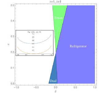
Figure 5: The new phase diagram. resetting rate $r=1$, interaction interval $\tau=1$. The green region is the information-eraser region, in which the demon is able to reduce the information entropy of the memory tape. The purple region is the refrigerator region, where the demon can help to produce anomalous work by exploiting information. The blue region is a dual-function region, both of the information erasing and anomalous work production functions could be realized in this region. The white part is the dub region. The inset shows a demonstration of the generalized second law, where the dynamical parameter $\epsilon$ is fixed to be $0.06$. The yellow line corresponds to the line of original second law without considering the contribution from resetting, the blue line corresponds to the generalized second law including the resetting work term $W_{r}$.

Generalized second law in the presence of resetting

The dual-function region in the new phase diagram shows that the autonomous demon with resetting seems to be against the second law of thermodynamics. To address this issue, a generalized second law is derived by constructing a Lyapunov function, or by using the integral fluctuation theorem for stochastic entropy production (see Appendix E for details).

As a result, the generalized second law of thermodynamics of the system with resetting in the periodic steady state is demonstrated to be

$$Q_{c\rightarrow h}(\beta_{h}-\beta_{c})+\Delta S_{B}+\beta_{h}W_{\tau}^{r}\geq 0,$$ (29)

where the $W_{\tau}^{r}$ is the ’resetting work’ during an interval $[n\tau,(n+1)\tau]$ due to stochastic resetting. This generalized second law is our third main result. The new term $W_{\tau}^{r}$ is the cost for resetting, and for the information refrigerator it is given by

$$W_{\tau}^{r}=k_{B}T_{h}\Delta S_{D}+\Delta p^{D,ps}\Delta E.$$ (30)

Here, $\Delta p^{D,ps}\equiv p_{\tau,u}^{D,ps}-p_{\text{in},u}^{D,ps}$ denotes the difference between the steady state probability of the demon in up state at the final moment and at the initial moment within an interval. From the expression, we can see that this new term contributed by resetting consists of two parts. The first part is the Shannon entropy difference between the initial distribution and the final distribution in each interaction interval, which is an extra entropic cost. The second part $\beta_{h}\Delta p^{D,ps}\Delta E$ can be interpreted as the energy cost needed to maintain this distribution difference between the demon at the final moment and at the initial moment, or say, to maintain the new periodic steady state. To demonstrate the generalized second law, we further fix $\epsilon$ to be $0.06$ and plot the $Q_{c\rightarrow h}(\beta_{h}-\beta_{c})+\Delta S_{B}$ and $Q_{c\rightarrow h}(\beta_{h}-\beta_{c})+\Delta S_{B}+\beta_{h}W_{\tau}^{r}$ respectively as functions of $\epsilon$ in the inset of Fig. 5. The yellow line corresponds to the original second law without considering the effect of resetting, and the blue line corresponds to the generalized second law. It can be seen that part of the yellow line is below zero, which means the original second law is violated. What’s more, using the so-called thermodynamic uncertainty relation (TUR) Barato and Seifert (2015); Gingrich et al. (2016); Polettini et al. (2016); Liu et al. (2020); Koyuk and Seifert (2020), a relation stronger than the generalized second law (29) may be obtained.

From this expression (30) we may explain physically why the down state $\vec{\Delta}=(0,1)^{\text{T}}$ should be chosen as the resetting state to improve the engine’s performance, instead of the up state $\vec{\Delta}=(1,0)^{\text{T}}$ or any mixed state. Actually the down state may be the best selection that can optimize the performance of the information refrigerator. To better the comprehensive performance of the information refrigerator, larger cost from resetting $W_{\tau}^{r}$ is preferred, because the larger the cost is, the bigger the anomalous energy transfer $Q_{c\rightarrow h}$ and the smaller the entropy difference $\Delta S_{B}$ can be. Therefore, the optimal resetting mechanism should maximize the $\Delta p^{D,ps}$ and the $\Delta S_{D}$ simultaneously. If the demon is reset to a given mixed state like $(1/2,1/2)^{\text{T}}$, the initial Shannon entropy $S_{D,0}$ would take the maximal value, making $\Delta S_{D}<0$. Compared to this, reset the demon to a single state like $(0,1)^{\text{T}}$ or $(1,0)^{\text{T}}$ would make the Shannon entropy of the demon at the initial moment of an interval being zero, always following with $\Delta S_{D}>0$. Thus resetting the demon to a single state could be superior to resetting it to a mixed state. On the other hand, if the demon is reset to the up state at the start of each interval, the probability of it being in up state initially turns to be $1$, leading $\Delta p^{D,ps}$ to equals $p_{\tau,u}^{D,ps}-1<0$, which have negative impact in the refrigerator’s performance. Contrarily, the down-state reset still bring about the positive effect for this term as $\Delta p^{D,ps}=p_{\tau,u}^{D,ps}>0$. In consequence, picking the down state $(0,1)^{\text{T}}$ as the reset state rather than other states seems to be the optimal strategy.

V Discussion

Autonomous Maxwell’s demons have been paid much attention to in the field of small-system thermodynamics since Mandal and Jarzynski declared their exactly solvable model in 2012. It should be noted that the evolution of the memory tape is under some kind of resetting mechanism, i.e. the state of the tape is always being reset to a given initial statistical state after a fixed time $\tau$. Therefore, it would be intriguing to let the demon exposed to stochastic resetting as the bit does, which may serve as a strategy improving the demon’s performances. It has been shown that resetting protocol can be devised to optimize some dynamical processes Evans et al. (2020); Gupta and Jayannavar (2022); Busiello et al. (2021), thus it might be a promising idea to reset the demon randomly. However, most existing frameworks of stochastic resetting only deal with the continuous-time Markov process, which aren’t applicable to our case. Because the reset of the demon is only wanted to happen at the end of some interaction intervals.

In this article, we generalize the stochastic resetting formalism to discrete-time Markov process, so that this mechanism can be introduced to the autonomous Maxwell’s demon system, providing some novel designing principles and strategies. The time cost for the autonomous demon to relax to its working state (the periodic steady state) hasn’t been taken into account in the previous works. In reality, minimizing this time cost for the relaxation processes before the working state would be preferred. Using stochastic resetting mechanism, we provide some designing principles to optimize this relaxation process, minimizing the time cost to enter the working state through a protocol inspired by the strong Mpemba effect. Furthermore, we construct new functional states with remarkable features by keeping resetting the demon, and derive a generalized second law of thermodynamics including the contribution from discrete-time stochastic reset. We have illustrated our designing strategies in two autonomous demon models, the two-state Maxwell’s refrigerator and the three-state information heat engine.

An interesting open problem is the generalization of our framework to the case of time-dependent resetting rate, where the waiting time distribution of two consecutive resetting events is not an exponential distribution. To find other waiting time distributions which can improve the performance of the autonomous demon, it is really worthy of further study. Moreover, the stochastic resetting in quantum system is recently of wide interest Ruoyu Yin (2022); Perfetto et al. (2021), thus it would be promising to develop a framework as the quantum counterpart of our discrete-time resetting framework, which may further serve as a useful tool to analyze resetting mechanism in quantum systems.

Appendix

Appendix A Modified dynamics under stochastic resetting

Here we provide some details for the derivation of the equation (19) and (23) in the main text.

Plugging the expansion formula

$$\bm{p}_{\text{\text{in}}}^{D}(t_{N})=p_{\text{in}}^{D,ps}+\sum_{i\geq 2}a_{i}\lambda_{i}^{n}\bm{R}_{i}$$

and

$$\vec{\Delta}_{n\tau}=\bm{p}_{\text{in}}^{D,ps}+\sum_{i\geq 2}d_{i}\lambda_{i}^{n}\bm{R}_{i}$$

into the renewal equation (12) for the demon’s initial distribution:

$$\bm{p}_{\text{in}}^{D}(r,t_{N})=e^{-rN\tau}\bm{p}_{\text{in}}^{D}(t_{N})+\left(1-e^{-r\tau}\right)\sum_{n=0}^{N-1}\left[e^{-rn\tau}\vec{\Delta}_{n\tau}\right],$$

we reach that

$$\bm{p}^{D}(r,t_{N})= e^{-rN\tau}\left[\bm{p}_{\text{in}}^{D,ps}+\sum_{i\geq 2}a_{i}\lambda_{i}^{n}\bm{R}_{i}\right]+\left(1-e^{-r\tau}\right)\sum_{n=0}^{N-1}e^{-rn\tau}\left[\bm{p}_{\text{in}}^{D,ps}+\sum_{i\geq 2}d_{i}\lambda_{i}^{n}\bm{R}_{i}\right]$$ (31)

$$= \left[\bm{p}_{\text{in}}^{D,ps}+\sum_{i\geq 2}\frac{1-e^{-r\tau}}{1-\lambda_{i}e^{-r\tau}}d_{i}\bm{R}_{i}\right]+\sum_{i\geq 2}\left[a_{i}-\frac{1-e^{-r\tau}}{1-\lambda_{i}e^{-r\tau}}d_{i}\right]e^{-rN\tau}\lambda_{i}^{N}\bm{R}_{i}$$ (32)

$$= \bm{p}_{\text{in}}^{D,ps}+\sum_{i\geq 2}\left\{\left[a_{i}-\frac{d_{i}\left(1-e^{-r\tau}\right)}{1-\lambda_{i}e^{-r\tau}}\right]e^{-rN\tau}+\frac{d_{i}\left(1-e^{-r\tau}\right)}{1-\lambda_{i}e^{-r\tau}}\cdot\lambda_{i}^{-N}\right\}\lambda_{i}^{N}\bm{R}_{i}$$ (33)

$$\equiv \bm{p}_{\text{in}}^{D,ps}+\sum_{i\geq 2}a_{i}(r,N)\lambda_{i}^{N}\bm{R}_{i}.$$ (34)

Here, the modified coefficients $a_{i}(r,N)$ is obtained as

$$a_{i}(r,N)=\left[a_{i}-\frac{d_{i}\left(1-e^{-r\tau}\right)}{1-\lambda_{i}e^{-r\tau}}\right]e^{-rN\tau}+\frac{d_{i}\left(1-e^{-r\tau}\right)}{1-\lambda_{i}e^{-r\tau}}\cdot\lambda_{i}^{-N},$$

and the Eq. (32) gives rise to the initial distribution of demon’s new periodic steady state as

$$\bm{p}_{\text{in}}^{D,ps}(r)=\lim_{N\rightarrow\infty}\bm{p}^{D}(r,t_{N})=\bm{p}_{\text{in}}^{D,ps}+\sum_{i\geq 2}\frac{1-e^{-r\tau}}{1-\lambda_{i}e^{-r\tau}}d_{i}\bm{R}_{i},$$ (35)

which is the Eq. (23) in the main text.

Appendix B Details of information refrigerator

Extra details of the original information refrigerator

The transition matrix of the four-state combined system in this model is given by

$$\bm{R}=\begin{pmatrix}-\Gamma(1+\sigma)&\Gamma(1-\sigma)&0&0\\ \Gamma(1+\sigma)&-\left[1-\omega+\Gamma(1-\sigma)\right]&1+\omega&0\\ 0&1-\omega&-\left[1+\omega+\Gamma(1+\sigma)\right]&\Gamma(1-\sigma)\\ 0&0&\Gamma(1+\sigma)&-\Gamma(1-\sigma)\end{pmatrix}$$

Solution to the periodic steady state the expression of average production is as follow: the evolution matrix for initial distribution of the demon is given by

$$\mathcal{T}=\mathcal{P}^{D}e^{\mathcal{R}\tau}\mathcal{M},\mathcal{\ P}^{D}=\begin{pmatrix}1&0&1&0\\ 0&1&0&1\end{pmatrix},\ \mathcal{M}=\begin{pmatrix}p_{0}&0\\ 0&p_{0}\\ p_{1}&0\\ 0&p_{1}\end{pmatrix}$$

Then the periodic steady state $\bm{p}_{\text{in}}^{D,ps}$ for demon can be obtained by solving the linear equation

$$\mathcal{T}\bm{p}_{\text{in}}^{D,ps}=\bm{p}_{\text{in}}^{D,ps}.$$

In the periodic steady state, the joint distribution of the demon and the interacting bit, at the end of the interaction interval, is given by $\bm{p}_{\tau}^{ps}=e^{\mathcal{R}\tau}\mathcal{M}\bm{p}_{\text{in}}^{D,ps}$. The marginal distribution of the outgoing bit is then given by projecting out the state of the demon:

$$\bm{p}_{\tau}^{B,ps}=(p_{0}^{f},p_{1}^{f})=\mathcal{P}^{B}e^{\mathcal{R}\tau}\mathcal{M}\bm{p}_{\text{in}}^{D},\mathcal{P}^{B}=\begin{pmatrix}1&1&0&0\\ 0&0&1&1\end{pmatrix}.$$ (36)

Notice that $\bm{p}_{\text{in}}^{D,ps}$ is the first right eigenvector of $\mathcal{T}$, $\bm{p}_{\tau}^{B,ps}=(p_{0}^{f},p_{1}^{f})$ then can be solved, which determines the value of average production as $\Phi=p_{1}^{f}-p_{1}$. By performing these calculations using Mathematica,

$$\Phi=\frac{\delta-\epsilon}{2}\eta(\Lambda),\eta(\Lambda)=\frac{\nu_{2}P+\nu_{3}Q}{P+Q},$$ (37)

$$P=\mu_{2}(\mu_{4}\nu_{3}+\mu_{1}\nu_{1}),Q=\mu_{3}(\mu_{4}\nu_{2}+\mu_{1}\nu_{1}),$$ (38)

where

$$\nu_{1}=1-e^{-2\Gamma\tau},\nu_{2}=1-e^{-(1+\Gamma-\alpha)\tau},\nu_{2}=1-e^{-(1+\Gamma+\alpha)\tau},$$ (39)

$$\mu_{1}=(\delta+\sigma)\omega,\mu_{2}=\alpha+\Gamma+\sigma\omega,\mu_{3}=\alpha-\Gamma-\sigma\omega,\mu_{4}=1-\delta\omega$$ (40)

with $\alpha=\sqrt{1+\Gamma^{2}+2\Gamma\sigma\omega}$.

Appendix C Spectral analysis of the matrix $\mathcal{T}$

In this appendix, we gives some descriptions of the eigenvector expansion method used in the main text,i.e., doing spectral analysis of the evolution matrix $\mathcal{T}$ for the demon. $\mathcal{T}$ has right eigenvectors $\bm{R}_{i}$

$$\mathcal{T}\bm{R}_{i}=\lambda_{i}\bm{R}_{i}$$ (41)

and left eigenvectors $\bm{L}_{i}$ as

$$\bm{L}_{i}^{\text{T}}\mathcal{\mathcal{T}}=\lambda_{i}\bm{L}_{i}^{\text{T}}$$ (42)

with $\lambda_{i}$ the eigenvalues, which are sorted as $1=\lambda_{1}>\left|\lambda_{2}\right|\geq\left|\lambda_{3}\right|\geq...$ (we assume that $\lambda_{1}$ is not degenerate). The right eigenvector $\bm{R}_{1}$ with $1=\lambda_{1}$ corresponds to the periodic steady state, so we write $\bm{R}_{1}=\bm{p}_{\text{\text{in}}}^{D,ps}$. According to the completeness relation, the initial state $\bm{p}_{\text{\text{in}}}^{D}$ can be expanded as

$$\bm{p}_{\text{in,}0}=\bm{p}_{\text{in}}^{D,ps}+\sum_{i>1}d_{i}\bm{R}_{i},$$ (43) where $$d_{i}=\frac{\bm{L}_{i}^{\text{T}}\cdot\bm{p}_{\text{in,0}}^{D}}{\bm{L}_{i}^{\text{T}}\cdot\bm{R}_{i}}.$$ (44) Calculation of the $i^{th}$ coefficient $d_{i}$

For an arbitrary matrix $T$, it can be demonstrated that any pair of left eigenvector and right eigenvector corresponding to different eigenvalues of the matrix are mutually orthogonal. Here is the proof (no degeneracy):

$$T\bm{R}_{i} =\lambda_{i}\bm{R}_{i}\Rightarrow\begin{cases}\bm{L}_{j}^{\text{T}}T\bm{R}_{i}&=\lambda_{i}\bm{L}_{j}^{\text{T}}\bm{R}_{i}\\ \bm{L}_{j}^{\text{T}}T\bm{R}_{i}&=\lambda_{j}\bm{L}_{j}^{\text{T}}\bm{R}_{i}\end{cases}$$

$$\Rightarrow (\lambda_{i}-\lambda_{j})\bm{L}_{j}^{\text{T}}\bm{R}_{i}=0$$

$$\Rightarrow \bm{L}_{j}^{\text{T}}\bm{R}_{i}=(\bm{L}_{i}^{\text{T}}\cdot\bm{R}_{i})\delta_{ij}.$$

Therefore, for an evolution starting at a given initial distribution $\bm{p}_{\text{in}}^{D}$, we have that $d_{i}$ is the corresponding overlap coefficient between the initial probability and the $i^{th}$ left eigenvector $\bm{L}_{i}^{\text{T}}$. During the relaxation process, the initial distribution of the demon of the $n^{th}$ time interval, $\mathcal{T}^{n}\bm{p}_{\text{in,}0}^{D}$, can be written as

$$\mathcal{T}^{n}\bm{p}_{\text{\text{in,0}}}^{D}=\bm{p}_{\text{in}}^{D,ps}+\sum_{i>1}d_{i}\lambda_{i}^{n}\bm{R}_{i}.$$ (45)

Then,

$$\left\|\mathcal{T}^{n}\bm{p}_{\text{\text{in},0}}^{D}-\bm{p}_{\text{\text{in}}}^{D,ps}\right\|_{q}=\sum_{i>1}d_{i}\left\|\lambda_{i}\right\|_{q}^{n}\left\|R_{i}\right\|_{q}.$$ (46)

The relaxation timescale is typically characterized by

$$\tau_{\text{rel}}=-\frac{1}{\ln\left|\lambda_{2}\right|}.$$ (47)

It is then can be observed that a stronger effect (even shorter relaxation time) can occur: a process where there exists a specific initial distribution $\bm{\pi}_{\text{\text{in,0}}}^{D}$, such that

$$d_{2}|_{\bm{p}_{\text{\text{in},0}}^{D}=\bm{\pi}_{\text{\text{in,0}}}^{D}}=\frac{\bm{L}_{2}^{\text{T}}\cdot\bm{\pi}_{\text{in,0}}^{D}}{\bm{L}_{2}^{\text{T}}\cdot\bm{R}_{2}}=0.$$

Appendix D Eigenvalues of the information refrigerator model

Here we provide the expressions for the eigenvalues of the transition matrices for the two-state demon model.

For the two-state demon, in the case of $\Gamma=1,\ \omega=1/2$ the eigenvalues for $\mathcal{T}_{2\times 2}$ reads

$$\lambda_{1} =1,$$

$$\lambda_{2} =\frac{e^{-2\tau}\left[-4+e^{s\tau}\left(-2+s\right)\left(-2+\delta\right)\left(-2+\epsilon\right)-e^{-s\tau}\left(2+\delta\right)\left(-2+\epsilon\right)+4\delta\left(-2+\epsilon\right)+8\epsilon\right]}{4(4\epsilon-5)},$$ (48)

$$s \equiv\sqrt{2+\frac{1-2\epsilon}{2-\epsilon}}$$ (49)

We draw the contour plot (which is not shown here) for $\lambda_{2}$ with $\tau=1$ and show that $\lambda_{2}$ is positive for any value of $\epsilon\in[0,1/2]$ and $\delta\in[-1,1]$. It’s obvious that the sign of $\lambda_{2}$ is irrelevant to the value of $\tau$, thus the necessary condition for the existence of $N_{c}>0$, i.e. $\lambda_{2}>0$ can always be satisfied in this model.

Appendix E Derivation of the generalized second law of thermodynamics

During any interaction interval, the joint distribution of the interacting bit and the demon evolves according to the master equation

$$\frac{d\bm{p}}{dt}=\mathcal{R}\bm{p}.$$

Imagine that the interaction time $\tau$ is long enough ($\tau\rightarrow\infty$), then the combined system will finally reach a steady state (the entries of transition matrix $\mathcal{R}$ satisfy detailed balance condition, so it’s an equilibrium state)

$$\bm{p}^{ss}=\frac{(1,\mu,\mu\nu,\mu^{2}\nu)^{T}}{1+\mu+\mu\nu+\mu^{2}\nu},\mu=\frac{1+\sigma}{1-\sigma},\nu=\frac{1-\omega}{1+\omega},$$ (50)

which makes $\mathcal{R}\bm{p}^{ss}=\bm{0}.$ When $\tau\rightarrow\infty$, the steady state joint distribution $\bm{p}_{ss}$ is factorized as the product of marginal distributions $\bm{p}^{D,ss}$ and $\bm{p}^{B,ss}$, because the demon and bit are uncorrelated at the beginning of each interval by construction. And in this case distribution of bits can be regarded as an ’effective initial distribution’. That is,

$$p_{ij}^{ss}=p_{i}^{D,ss}p_{j}^{B,ss},\ \ i\in\{u,d\},\ \ j\in\{0,1\},$$ (51)

where $\bm{p^{D,ss}}=(1,\mu)^{T}/(1+\mu)$ and $\bm{p^{B,ss}}=(1,\mu\nu)^{T}/(1+\mu\nu).$ When interaction time $\tau$ is finite, the combined system always relaxes towards this final steady state, though being interrupted by the advent of new bits and stochastic resetting events (one should note the similarity between resetting events for the demon and comings of new bits). Therefore, the distribution of combined system will get closer to the steady state $\bm{p}_{ss}$ at the end of an interval, compared to its distribution at the start of the same interval. That is, the relative entropy between any state $\bm{p}$ of the combined system and the steady state $\bm{p}_{ss}$

$$D(\bm{p}||\bm{p}_{ss}) =\sum_{k}p_{k}\ln\frac{p_{k}}{p_{k}^{ss}}\geq 0,$$ (52)

$$k\in \{0u,0d,1u,1d\}$$ (53)

as a distance function is a Lyapunov function, satisfying

$$\frac{d}{dt}D(\bm{p}||\bm{p}_{ss})\leq 0\text{.}$$ (54)

Let $\bm{p}_{\text{in}}$ and $\bm{p}_{\tau}$ denote the joint distribution at the start and at the end of a given interval respectively, and similarly define $\bm{p}_{\text{in}}^{D}$, $\bm{p}_{\tau}^{D}$, $\bm{p}_{\text{in}}^{B}$ and $\bm{p}_{\tau}^{B}$ for the marginal distributions of the demon and the bit. Then equation (54) tells that

$$D(\bm{p}_{\text{in}}||\bm{p}_{ss})-D(\bm{p}_{\tau}||\bm{p}_{ss})\geq 0,$$ (55)

whose physical interpretation is the initial joint state is farther from steady state than the final state at the end of the given interval is. Note that the left hand side of the above equation is a standard expression of conventional entropy production during a period of time $\tau$ Shiraishi and Saito (2019):

$$\text{$\Sigma{}_{[0,\tau]}^{\textrm{tot}}\equiv$}D(\bm{p}_{\text{in}}||\bm{p}_{ss})-D(\bm{p}_{\tau}||\bm{p}_{ss})\geq 0.$$

Using (50) and (52) one can rewrite the above equation as

$$S_{\tau}-S_{0}+\sum_{i\in\{u,d\}}\left(p_{\tau,i}^{D}-p_{\text{in},i}^{D}\right)\ln p_{i}^{D,ss}$$

$$+\sum_{i\in\{0,1\}}\left(p_{\tau,i}^{B}-p_{\text{in},i}^{B}\right)\ln p_{i}^{B,ss} \geq 0,$$ (56)

where $S_{0}$ and $S_{\tau}$ refer to the information entropies of the joint distribution at the start and at the end of the current interval. What we need to consider is just the new periodic steady state in the presence of resetting. In this case, from the definition of the average production with resetting $\phi_{r}$, $p_{\tau,1}^{B}-p_{\text{in},1}^{B}=-(p_{\tau,0}^{B}-p_{\text{in},0}^{B})=\phi_{r}$, the last term of (56) can be rewritten as

$$\sum_{i\in\{0,1\}}\left(p_{\tau,i}^{B}-p_{\text{in},i}^{B}\right)\ln p_{i}^{B,ss} =\phi_{r}\ln\mu\nu$$ (57)

$$=Q_{c\rightarrow h}(\beta_{h}-\beta_{c})\text{.}$$ (58)

The joint information entropy $S$ can be decomposed as

$$S=S_{D}+S_{B}+I(D;B),\ \ \ I(D;B)\geq 0,$$ (59)

where $S_{D}$ and $S_{B}$ are marginal information entropy of the demon and the bit. Thus in our NPSS with resetting, equation (56) gives (note that $I_{0}(D;B)=0$ due to the uncorrelated initial distribution)

$$Q_{c\rightarrow h}(\beta_{h}-\beta_{c})+\Delta S_{B}+\beta_{h}W_{\tau}^{r}\geq I_{\tau}(D;B)\geq 0,$$ (60)

where

$$\Delta S_{B}= S_{B,\tau}-S_{B,0}$$ (61)

$$= S_{B}(\delta^{\prime})-S_{B}(\delta)=S_{B}(\delta-2\phi_{\text{tot}})-S_{B}(\delta),$$

$$S_{B}(\delta)= -\sum_{i=0}^{1}p_{i}\ln p_{i}$$

$$= -\frac{1-\delta}{2}\ln\frac{1-\delta}{2}-\frac{1+\delta}{2}\ln\frac{1+\delta}{2},$$ (62)

$$(\delta =p_{0}-p_{1},\ \delta^{{}^{\prime}}=p_{0}^{{}^{\prime}}-p_{1}^{{}^{\prime}})$$ (63)

and

$$W_{\tau}^{r} \equiv\Delta S_{D}+\sum_{i\in\{u,d\}}\left(p_{\tau,i}^{D,ps}-p_{\text{in},i}^{D,ps}\right)\ln p_{i}^{D,ss},$$ (64)

$$\Delta S_{D} =-\sum_{i=d}^{u}p_{\tau,i}^{D,ps}\ln p_{\tau,i}^{D,ps}+\sum_{i=d}^{u}p_{\text{in},i}^{D,ps}\ln p_{\text{in},i}^{D,ps}$$ (65)

is the ’resetting work’ during a whole interval $[n\tau,(n+1)\tau]$ due to stochastic resetting. In the original periodic steady state without resetting, one has $\bm{p}_{\tau}^{D,ps}=\mathcal{T}\bm{p}_{\text{in}}^{D,ps}=\bm{p}_{\text{in}}^{D,ps}$ from definition of this state, so that the dissipated work (64) vanishes. However, in the NPSS $\bm{p}_{\tau}^{D,ps}(r)=\mathcal{T}\bm{p}_{\text{in}}^{D,ps}(r)\neq\bm{p}_{\text{in}}^{D,ps}(r)$ according to the definition (23). In the NPSS, one can obtain

$$\bm{p}_{\tau}^{D,ps}(r)-\bm{p}_{\text{in}}^{D,ps}(r)=\mathcal{T}\bm{p}_{\text{in}}^{D,ps}(r)-\bm{p}_{\text{in}}^{D,ps}(r)$$ (66)

$$=\frac{1-e^{-r\tau}}{1-\lambda_{2}e^{-r\tau}}d_{2}\left(\mathcal{T}\bm{R}_{2}-\bm{R}_{2}\right)$$ . (67)

Because $p_{\tau,u}^{D,ps}-p_{\text{in},u}^{D,ps}=-(p_{\tau,d}^{D,ps}-p_{\text{in},d}^{D,ps})\equiv\Delta p^{D,ps}$, the second contribution of resetting work can be written as

$$\sum_{i=d}^{u}\left(p_{\tau,i}^{D,ps}-p_{0,i}^{D,ps}\right)\ln p_{i}^{D,ss} =\Delta p^{D,ps}\ln\mu$$

$$=\beta_{h}\Delta p^{D,ps}\Delta E,$$ (68)

thus the resetting work during each interval in the NPSS is given by

$$W_{\tau}^{r}=\Delta S_{D}+\beta_{h}\Delta p^{D,ps}\Delta E.$$ (69)

The above modified second law can also be derived from an integral fluctuation theorem for the stochastic entropy production. Following Seifert’s spirit, the total stochastic entropy production in an interaction interval for a single trajectory $\Gamma_{i\rightarrow j}$ starting in state $i$ at initial time and ending in state $j$ at time $\tau$ is defined as ($i,j\in\{0u,0d,1u,1d\}$)

$$\sigma(\Gamma_{i\rightarrow j})= \ln\frac{p_{i}(0)p(\Gamma_{i\rightarrow j})}{p_{j}(\tau)p(\Gamma_{j\rightarrow i}^{\dagger})},$$ (70)

$$= \ln\left[\frac{p_{i}(0)}{p_{j}(\tau)}\prod_{k,l\in\Gamma_{i\rightarrow j}}\left(\frac{R_{kl}}{R_{lk}}\right)^{n_{kl}}\right],$$ (71)

which naturally gives rise to an integral fluctuation theorem

$$\langle e^{-\sigma(\Gamma_{i\rightarrow j})}\rangle= \sum_{i,j}\int d\Gamma_{i\rightarrow j}p_{i}(0)p(\Gamma_{i\rightarrow j})e^{-\sigma(\Gamma_{i\rightarrow j})}$$

$$= \sum_{i,j}\int d\Gamma_{i\rightarrow j}p_{j}(\tau)p(\Gamma_{j\rightarrow i}^{\dagger})$$

$$= \sum_{i,j}\int d\Gamma_{j\rightarrow i}^{\dagger}p_{j}(\tau)p(\Gamma_{j\rightarrow i}^{\dagger})=1.$$ (72)

Then using Jensen equality, it follows that

$$\Sigma{}_{[0,\tau]}^{\textrm{tot}}\equiv\langle\sigma(\Gamma_{i\rightarrow j})\rangle\geq 0.$$

It has been proven that Seifert (2012)

$$\langle\frac{d}{dt}\sigma(\Gamma_{i\rightarrow j})\rangle=\left[R_{ij}p_{j}(t)-R_{ji}p_{i}(t)\right]\ln\frac{R_{ij}p_{j}(t)}{R_{ji}p_{i}(t)}$$ (73)

Then we have

$$\langle\sigma(\Gamma_{i\rightarrow j})\rangle= \int_{0}^{\tau}\sum_{i>j}\left[R_{ij}p_{j}(t)-R_{ji}p_{i}(t)\right]\ln\frac{R_{ij}p_{j}(t)}{R_{ji}p_{i}(t)}$$

$$= -\int_{0}^{\tau}\frac{d}{dt}D(\bm{p}(t)||\bm{p}_{ss})$$

$$= Q_{c\rightarrow h}(\beta_{h}-\beta_{c})+\Delta S_{B}+\beta_{h}W_{\tau}^{r}-I_{\tau}(D;B)\geq 0,$$

where in the second line the detailed balance condition $R_{ij}p_{j}^{ss}=R_{ji}p_{i}^{ss}$ has been used Horowitz and England (2017).

References

- Maxwell and Pesic (1871) J. C. Maxwell and P. Pesic, Theory of heat (Courier Corporation, 1871).
- Landauer (1961) R. Landauer, IBM journal of research and development 5, 183 (1961).
- Bennett (1982) C. H. Bennett, International Journal of Theoretical Physics 21, 905 (1982).
- Rex (2017) A. Rex, Entropy 19, 240 (2017).
- Parrondo et al. (2015) J. Parrondo, J. M. Horowitz, and T. Sagawa, Nature Physics 11, 131 (2015).
- Szilard (1929) L. Szilard, Zeitschrift für Physik 53, 840 (1929).
- Feynman et al. (2011) R. P. Feynman, R. B. Leighton, and M. Sands, The Feynman lectures on physics, Vol. I: The new millennium edition: mainly mechanics, radiation, and heat, vol. 1 (Basic books, 2011).
- Mandal and Jarzynski (2012) D. Mandal and C. Jarzynski, Proceedings of the National Academy of Sciences 109, 11641 (2012).
- Sagawa and Ueda (2012) T. Sagawa and M. Ueda, Physical Review E 85, 021104 (2012).
- Mandal et al. (2013) D. Mandal, H. T. Quan, and C. Jarzynski, Physical review letters 111, 030602 (2013).
- Strasberg et al. (2014) P. Strasberg, G. Schaller, T. Brandes, and C. Jarzynski, Phys. Rev. E 90, 062107 (2014), URL https://link.aps.org/doi/10.1103/PhysRevE.90.062107.
- Koski et al. (2015) J. V. Koski, A. Kutvonen, I. M. Khaymovich, T. Ala-Nissila, and J. P. Pekola, Phys. Rev. Lett. 115, 260602 (2015), URL https://link.aps.org/doi/10.1103/PhysRevLett.115.260602.
- Jurgens and Crutchfield (2020) A. M. Jurgens and J. P. Crutchfield, Phys. Rev. Research 2, 033334 (2020), URL https://link.aps.org/doi/10.1103/PhysRevResearch.2.033334.
- Joseph and V. (2021) T. Joseph and K. V., Phys. Rev. E 103, 022131 (2021), URL https://link.aps.org/doi/10.1103/PhysRevE.103.022131.
- Debankur Bhattacharyya (2022) C. J. Debankur Bhattacharyya, arXiv preprint arXiv:2205.13304 (2022).
- He et al. (2022) L. He, A. Pradana, J. W. Cheong, and L. Y. Chew, Phys. Rev. E 105, 054131 (2022), URL https://link.aps.org/doi/10.1103/PhysRevE.105.054131.
- Sandberg et al. (2014) H. Sandberg, J.-C. Delvenne, N. J. Newton, and S. K. Mitter, Phys. Rev. E 90, 042119 (2014), URL https://link.aps.org/doi/10.1103/PhysRevE.90.042119.
- Manzano et al. (2021) G. Manzano, D. Subero, O. Maillet, R. Fazio, J. P. Pekola, and E. Roldán, Phys. Rev. Lett. 126, 080603 (2021), URL https://link.aps.org/doi/10.1103/PhysRevLett.126.080603.
- Nahuel Freitas (2022) M. E. Nahuel Freitas, arXiv preprint arXiv:2204.09466 (2022).
- Ryu et al. (2022) S. Ryu, R. López, and R. Toral, New Journal of Physics 24, 033028 (2022), URL https://doi.org/10.1088/1367-2630/ac57ea.
- Deffner (2013) S. Deffner, Phys. Rev. E 88, 062128 (2013), URL https://link.aps.org/doi/10.1103/PhysRevE.88.062128.
- Poulsen et al. (2022) K. Poulsen, M. Majland, S. Lloyd, M. Kjaergaard, and N. T. Zinner, Phys. Rev. E 105, 044141 (2022), URL https://link.aps.org/doi/10.1103/PhysRevE.105.044141.
- Evans and Majumdar (2011) M. R. Evans and S. N. Majumdar, Phys. Rev. Lett. 106, 160601 (2011), URL https://link.aps.org/doi/10.1103/PhysRevLett.106.160601.
- Gupta et al. (2014) S. Gupta, S. N. Majumdar, and G. Schehr, Phys. Rev. Lett. 112, 220601 (2014), URL https://link.aps.org/doi/10.1103/PhysRevLett.112.220601.
- Reuveni (2016) S. Reuveni, Phys. Rev. Lett. 116, 170601 (2016), URL https://link.aps.org/doi/10.1103/PhysRevLett.116.170601.
- Pal and Reuveni (2017) A. Pal and S. Reuveni, Phys. Rev. Lett. 118, 030603 (2017), URL https://link.aps.org/doi/10.1103/PhysRevLett.118.030603.
- Belan (2018) S. Belan, Phys. Rev. Lett. 120, 080601 (2018), URL https://link.aps.org/doi/10.1103/PhysRevLett.120.080601.
- Chechkin and Sokolov (2018) A. Chechkin and I. M. Sokolov, Phys. Rev. Lett. 121, 050601 (2018), URL https://link.aps.org/doi/10.1103/PhysRevLett.121.050601.
- Pal et al. (2019) A. Pal, I. Eliazar, and S. Reuveni, Phys. Rev. Lett. 122, 020602 (2019), URL https://link.aps.org/doi/10.1103/PhysRevLett.122.020602.
- Miron and Reuveni (2021) A. Miron and S. Reuveni, Phys. Rev. Research 3, L012023 (2021), URL https://link.aps.org/doi/10.1103/PhysRevResearch.3.L012023.
- De Bruyne et al. (2022) B. De Bruyne, S. N. Majumdar, and G. Schehr, Phys. Rev. Lett. 128, 200603 (2022), URL https://link.aps.org/doi/10.1103/PhysRevLett.128.200603.
- De Bruyne et al. (2020) B. De Bruyne, J. Randon-Furling, and S. Redner, Phys. Rev. Lett. 125, 050602 (2020), URL https://link.aps.org/doi/10.1103/PhysRevLett.125.050602.
- Roldán et al. (2016) E. Roldán, A. Lisica, D. Sánchez-Taltavull, and S. W. Grill, Phys. Rev. E 93, 062411 (2016), URL https://link.aps.org/doi/10.1103/PhysRevE.93.062411.
- Busiello et al. (2021) D. M. Busiello, D. Gupta, and A. Maritan, New Journal of Physics 23, 103012 (2021), URL https://doi.org/10.1088/1367-2630/ac2922.
- Gupta et al. (2020) D. Gupta, C. A. Plata, and A. Pal, Phys. Rev. Lett. 124, 110608 (2020), URL https://link.aps.org/doi/10.1103/PhysRevLett.124.110608.
- Busiello et al. (2020) D. M. Busiello, D. Gupta, and A. Maritan, Phys. Rev. Research 2, 023011 (2020), URL https://link.aps.org/doi/10.1103/PhysRevResearch.2.023011.
- Gupta and Busiello (2020) D. Gupta and D. M. Busiello, Phys. Rev. E 102, 062121 (2020), URL https://link.aps.org/doi/10.1103/PhysRevE.102.062121.
- Pal et al. (2021) A. Pal, S. Reuveni, and S. Rahav, Phys. Rev. Research 3, 013273 (2021), URL https://link.aps.org/doi/10.1103/PhysRevResearch.3.013273.
- Fuchs et al. (2016) J. Fuchs, S. Goldt, and U. Seifert, EPL (Europhysics Letters) 113, 60009 (2016).
- Pal and Rahav (2017) A. Pal and S. Rahav, Phys. Rev. E 96, 062135 (2017), URL https://link.aps.org/doi/10.1103/PhysRevE.96.062135.
- Evans et al. (2020) M. R. Evans, S. N. Majumdar, and G. Schehr, J. Phys. A: Math. Theor 53, 193001 (2020).
- Gupta and Jayannavar (2022) S. Gupta and A. M. Jayannavar, Frontiers in Physics 10, 789097 (2022).
- (43) Z. Cao, R. Bao, J. Zheng, and Z. Hou, to be published.
- Gal and Raz (2020) A. Gal and O. Raz, Physical review letters 124, 060602 (2020).
- Klich et al. (2019) I. Klich, O. Raz, O. Hirschberg, and M. Vucelja, Physical Review X 9, 021060 (2019).
- Kumar and Bechhoefer (2020) A. Kumar and J. Bechhoefer, Nature 584, 64 (2020).
- Lu and Raz (2017) Z. Lu and O. Raz, Proceedings of the National Academy of Sciences 114, 5083 (2017).
- Santos and Prados (2020) A. Santos and A. Prados, Physics of Fluids 32, 072010 (2020).
- Baity-Jesi et al. (2019) M. Baity-Jesi, E. Calore, A. Cruz, L. A. Fernandez, J. M. Gil-Narvión, A. Gordillo-Guerrero, D. Iñiguez, A. Lasanta, A. Maiorano, E. Marinari, et al., Proceedings of the National Academy of Sciences 116, 15350 (2019).
- Meyer (2000) C. D. Meyer, Matrix analysis and applied linear algebra, vol. 71 (Siam, 2000).
- Barato and Seifert (2015) A. C. Barato and U. Seifert, Phys. Rev. Lett. 114, 158101 (2015), URL https://link.aps.org/doi/10.1103/PhysRevLett.114.158101.
- Gingrich et al. (2016) T. R. Gingrich, J. M. Horowitz, N. Perunov, and J. L. England, Phys. Rev. Lett. 116, 120601 (2016), URL https://link.aps.org/doi/10.1103/PhysRevLett.116.120601.
- Polettini et al. (2016) M. Polettini, A. Lazarescu, and M. Esposito, Phys. Rev. E 94, 052104 (2016), URL https://link.aps.org/doi/10.1103/PhysRevE.94.052104.
- Liu et al. (2020) K. Liu, Z. Gong, and M. Ueda, Phys. Rev. Lett. 125, 140602 (2020), URL https://link.aps.org/doi/10.1103/PhysRevLett.125.140602.
- Koyuk and Seifert (2020) T. Koyuk and U. Seifert, Phys. Rev. Lett. 125, 260604 (2020), URL https://link.aps.org/doi/10.1103/PhysRevLett.125.260604.
- Ruoyu Yin (2022) E. B. Ruoyu Yin, arXiv preprint arXiv:2205.01974 (2022).
- Perfetto et al. (2021) G. Perfetto, F. Carollo, M. Magoni, and I. Lesanovsky, Phys. Rev. B 104, L180302 (2021), URL https://link.aps.org/doi/10.1103/PhysRevB.104.L180302.
- Shiraishi and Saito (2019) N. Shiraishi and K. Saito, Phys. Rev. Lett. 123, 110603 (2019), URL https://link.aps.org/doi/10.1103/PhysRevLett.123.110603.
- Seifert (2012) U. Seifert, Reports on Progress in Physics 75, 126001 (2012).
- Horowitz and England (2017) J. M. Horowitz and J. L. England, Entropy 19, 333 (2017).