Guaranteed Privacy of Distributed Nonconvex Optimization via Mixed-Monotone Functional Perturbations

Abstract

In this paper, we introduce a new notion of guaranteed privacy that requires that the change of the range of the corresponding inclusion function to the true function is small. In particular, leveraging mixed-monotone inclusion functions, we propose a privacy-preserving mechanism for nonconvex distributed optimization, which is based on deterministic, but unknown, affine perturbation of the local objective functions, which is stronger than probabilistic differential privacy. The design requires a robust optimization method to characterize the best accuracy that can be achieved by an optimal perturbation. Subsequently, this is used to guide the refinement of a guaranteed-private perturbation mechanism that can achieve a quantifiable accuracy via a theoretical upper bound that is shown to be independent of the chosen optimization algorithm.

I Introduction

Data privacy and protection have become a critical concern in the management of cyber-physical systems (CPS) and their public trustworthiness. In such applications, malicious agents can expand their attack surface by extracting valuable information from the many physical, control, and communication components of the system, inflicting damage on the CPS and its users. Hence, a great effort is being devoted to design robust data-security control strategies for these systems [1]. Motivated by this, we aim to investigate an alternative design of privacy-preserving mechanisms, which can make the quantification of privacy, as well as the associated performance loss, both tractable and reasonable.

Literature Review. Among the many approaches to data security, one can distinguish privacy-aware methods that protect sensitive data from worst-case data breaches by adding random perturbations to it. However, this high data-resiliency can come at the cost of high performance loss, which either be hard to quantify in practice, or theoretically bounded by indices that are too large to be useful. A main approach to characterize this trade-off while preserving privacy in the literature is that of differential privacy [2].

This method was originally proposed for the protection of databases of individual records subject to public queries. In particular, a system processing sensitive inputs is made differentially private by randomizing its answers in such a way that the distribution over published outputs is not too sensitive to the data provided by any single participant. This notion has been extended to several areas in machine learning and regression  [3, 4, 5], control (estimation, verification) [6, 7], multi-agent systems (consensus, message passing) [8, 9, 10], and optimization and games [11, 12, 13], thereafter. In particular, a notable privacy-preserving mechanism design approach in the literature is based on the idea of message perturbation, i.e., modifying an original non-private algorithm by having agents perturb the messages/outputs to their neighbors or a central coordinator with Laplace or Gaussian noise [8, 9, 10]. This approach benefits from working with the original objective functions, however suffers from a steady-state accuracy error, since for fixed design parameters, the algorithm’s output does not correspond the true optimizer in the absence of noise [14].

Another notable approach to privacy relies on functional perturbation, with the idea of having agent(s) independently perturb their objective function(s) in a differentially private way and then participating in a centralized (distributed) algorithm [4, 3, 14]. The work in [3] proposed a differentially private classifier by perturbing the objective function with a linear finite-dimensional function. However, only the privacy of the underlying finite-dimensional parameter set–and not the entire objective functions–is preserved. A sensitivity-based differentially private algorithm was designed in [4] by perturbing the Taylor expansion of the cost function, where, unfortunately, the functional space had to be restricted to the space of quadratic functions. Similar perturbations proposed in [5] but without ensuring the smoothness and convexity of the perturbed function. In addition, none of  [3, 4, 5] provided a systematic way to study the effect of added noise on the global optimizer. To address this issue,  [14] suggested specific functional perturbations such that the difference between the probabilities of events corresponding to any pair of data sets is bounded by a function of the distance between the data sets, at the expense of a trade-off between the privacy and the accuracy of the mechanism. Further, the works in [7, 15] provided theoretically proven numerical methods to quantify differential privacy in high probability in estimation and verification, respectively. However, differential privacy inherently requires the slight change of the statistics of the output of the perturbed function or message if the objective function or the message sent from one agent changes. This, satisfies privacy only in a probabilistic, and not a guaranteed sense. To bridge this gap, we aim to investigate an alternative deterministic approach to privacy-preserving mechanism design, and also to relax the convexity assumption needed in most of the existing works.

Contributions. We start by introducing a novel notion of guaranteed privacy. This notion applies to deterministic, but unknown, functional perturbations of an optimization problem, and characterizes privacy in terms of how close the ranges of two sets of functions in a vicinity are. This notion of privacy is stronger than that of differential privacy in the sense that it guarantees that the change of the inclusion of the true function ranges is small, as opposed to looking at perturbed function statistics. By exploiting the differentiability and local Lipschitzness of the objective functions, we propose a novel perturbation mechanism that relies on the mixed-monotone inclusion functions of the problem objectives. We then characterize the best accuracy that can be achieved by an optimal perturbation, and use this to guide the refinement of a guaranteed-private, perturbation mechanism that can achieve a quantifiable accuracy via a theoretical upper bound. The design requires a robust optimization approach, and restricts privacy to functions in a given vicinity. Simulations are used to illustrate the level of the tightness of this bound for different nonconvex optimization algorithms, illustrating the accuracy-privacy compromise.

II Preliminaries

In this section, we introduce basic notation, as well as preliminary concepts and results used in the sequel.

Notation. $\mathbb{R}^{n},\mathbb{R}^{n\times p},\mathbb{D}_{n},{\color[rgb]{0,0,0}\mathbb{R}^{n}_{\geq 0}}$, and $\mathbb{R}^{n}_{>0}$ denote the $n$-dimensional Euclidean space, and the sets of $n$ by $p$ matrices, diagonal $n$ by $n$ matrices, and nonnegative and positive vectors in $\mathbb{R}^{n}$, respectively. Also, $\mathbf{0}_{n\times p},I_{n}$ and $\mathbf{0}_{n}$ denote the zero matrix in $\mathbb{R}^{n\times p}$, the identity matrix in $\mathbb{R}^{n\times n}$, and the zero vector in $\mathbb{R}^{n}$, respectively. Further, for $D\subseteq\mathbb{R}^{n}$, $L_{2}(D)$ denotes the set of square-integrable measurable functions over $D$. Given $M\in\mathbb{R}^{n\times p}$, $M^{\top}$ represents its transpose, $M_{ij}$ denotes $M$’s entry in the $i^{\textup{th}}$ row and the $j^{\textup{th}}$ column, $M^{\oplus}\triangleq\max(M,\mathbf{0}_{n\times p})$, $M^{\ominus}=M^{\oplus}-M$ and $|M|\triangleq M^{\oplus}+M^{\ominus}$. Finally, for $a,b\in\mathbb{R}^{n},a\leq b$ means $a_{i}\leq b_{i},\forall i\in\{1,\dots,n\}$.

Definition 1 (Hyper-intervals).

A (hyper-)interval $\mathcal{I}\triangleq[\underline{{\color[rgb]{0,0,0}z}},\overline{{\color[rgb]{0,0,0}z}}]\subset\mathbb{R}^{n}$, or an $n$-dimensional interval, is the set of all real vectors ${\color[rgb]{0,0,0}z\in\mathbb{R}^{n}}$ that satisfy $\underline{{\color[rgb]{0,0,0}z}}\leq{\color[rgb]{0,0,0}z}\leq\overline{{\color[rgb]{0,0,0}z}}$. Moreover, we call $\textstyle{\mathrm{diam}}(\mathcal{I})\triangleq\|\overline{{\color[rgb]{0,0,0}z}}-\underline{{\color[rgb]{0,0,0}z}}\|{\color[rgb]{0,0,0}_{\infty}\triangleq\max_{i\in\{1,\cdots,{\color[rgb]{0,0,0}n}\}}{\color[rgb]{0,0,0}|\overline{z}_{i}-\underline{z}_{i}|}}$ the diameter or interval width of $\mathcal{I}$. Finally, $\mathbb{IR}^{n}$ denotes the space of all $n$-dimensional intervals, i.e., interval vectors.

Definition 2 ($\mathcal{V}$-Adjacent Sets of Functions).

Given any normed vector space $(\mathcal{V};\|\cdot\|_{\mathcal{V}})$ with $\mathcal{V}\subseteq L_{2}(D)$, two sets of functions $F\triangleq\{f_{1},\dots,f_{n}\},F^{\prime}\triangleq\{f^{\prime}_{1},\dots,f^{\prime}_{n}\}\subset L_{2}(D)$ are called $\mathcal{V}$-adjacent if there exists $i_{0}\in\{1,\dots,n\}$ such that

$$f_{i_{0}}-f^{\prime}_{i_{0}}\in\mathcal{V},\quad\text{and}\quad f_{i}=f^{\prime}_{i},\text{ for all other }i\neq i_{0}\,.$$

III Problem Formulation

Consider a group of $N$ agents communicating over a network. Each agent $i\in\{1,\dots,{\color[rgb]{0,0,0}N}\}$ has a local objective function $\hat{f}_{i}:D\to\mathbb{R}$, where $D\subset\mathbb{R}^{n}$ has a nonempty interior. Consider the problem

$$\min_{x\in\mathcal{X}_{0}}\hat{f}(x)\triangleq\sum_{i=1}^{N}\hat{f}_{i}(x)\ \operatorname{s.t.}\ G(x)\leq 0,H(x)=b,x\in\mathcal{X}_{0},$$ (1)

where the mappings $G:D\to\mathbb{R}^{m},H:D\to\mathbb{R}^{s}$ are convex, the vector $b\in\mathbb{R}^{s}$ are known to all agents and $\mathcal{X}_{0}\triangleq[\underline{x}_{0},\overline{x}_{0}]$ is assumed to be an interval in $\mathbb{R}^{n}$. By applying a penalty method [16, Ch.5], the problem in (1) is equivalent to

$$\min_{x\in\mathcal{X}_{0}}f(x)\triangleq\sum_{i=1}^{N}f_{i}(x),$$ (2)

where, we assume the following:

Assumption 1 ( Locally Lipschitz, Differentiable and Private Objective Functions).

Each $f_{i}$ is differentiable, locally Lipschitz in its domain and only known to agent $i$. Moreover, upper and lower uniform bounds for its Jacobian matrix, $\overline{J}_{i}^{f},\underline{J}_{i}^{f}\in\mathbb{R}^{1\times{\color[rgb]{0,0,0}n}}$ are only known to agent $i$.

Note that we do not restrict any $f_{i},i\in\{1,\dots,n\}$, to be convex, nor twice-continuously differentiable. It is assumed that the problem constraint set $\mathcal{X}_{0}$ is globally known to each agent. The problem objective is to define a mechanism so that agents can solve (2) via a distributed, private algorithm.

It is known that even if $f_{i}$ and/or its gradient may not be directly shared among agents, an adversary may be able to infer it by compounding side information with network communications. This problem has been addressed via the notion of differential privacy and the design of differentially-private algorithms, e.g., in [14, 11, 12, 13], for convex objective functions (cf. Section I for a thorough review of the relevant work). Differential privacy applies a random, additive perturbation to either the algorithm input data or its output, so that the result becomes very close to that of the same process when applied to data in a vicinity. Here, our problem data refers to the problem objective functions, and the novel to-be-designed privacy mechanism consists of applying deterministic additive perturbations characterized by intervals—but unknown to the adversary. By doing so, the approximated range of the objective functions is also an interval, and privacy can be measured by how close these intervals are for functions in a vicinity. We formalize this via a mapping $\mathcal{M}$, as follows, and provide one such mapping in the next section.

Definition 3 (Guaranteed Privacy).

Let $\mathcal{M}:L_{2}(D)^{N}\times\mathbb{IR}^{n}\to\mathbb{IR}^{N}$ be a deterministic interval-valued map from the function space $L_{2}(D)^{N}$ to the space of intervals in $\mathbb{R}^{N}$. Given $\mathcal{X}\triangleq[\underline{x},\overline{x}]\in\mathbb{IR}^{n}$ and a “privacy gap” $\epsilon\in\mathbb{R}_{>0}$, the map $\mathcal{M}$ is $\epsilon$-guaranteed private with respect to the vicinity $\mathcal{V}$, if for any two $\mathcal{V}$-adjacent sets of functions $F\triangleq\{f_{i}\}_{i=1}^{N}$ and $F^{\prime}\triangleq\{f^{\prime}_{i}\}_{i=1}^{N}$ that (at most) differ in their $i_{0}^{\textup{th}}$ element and any interval $\mathcal{I}\in\mathbb{IR}^{N}$ such that $\mathcal{M}(F,{\color[rgb]{0,0,0}\mathcal{X}})\subseteq\mathcal{I}$, one has

$$\textstyle{\mathrm{diam}}{(\mathcal{M}(F^{\prime},{\color[rgb]{0,0,0}\mathcal{X}})\cap\mathcal{I})}\leq e^{\epsilon\|f_{i_{0}}-f^{\prime}_{i_{0}}\|_{\mathcal{V}}}\textstyle{\mathrm{diam}}{(\mathcal{M}(F,{\color[rgb]{0,0,0}\mathcal{X}}))}.$$ (3)

It is worth to reemphasize the difference between the notions of guaranteed privacy (introduced above) and differential privacy utilized in most of the work in the literature, e.g., [14, 11, 12]. When differential privacy is considered, the statistics of the output of $\mathcal{M}$, i.e., the probability of the value of $\mathcal{M}$ belonging to some set changes only relatively slightly if the objective function of one agent changes, and the change is in $\mathcal{V}$ (cf. [14, Definition III.1] for more details). On the other hand, when guaranteed privacy is considered, instead of introducing randomness to disguise the objective function, we implement a range perturbation of $\mathcal{V}$-adjacent functions as defined above, with the end goal of robustifying the optimization problem (2) in a controlled manner by an $\epsilon$ gap. This being said, note that our goal is to design a new mechanism (or mapping) $\mathcal{M}$ that preserves the $\epsilon$-guaranteed privacy of the objective functions with respect to the problem solution, regardless of the distributed (nonconvex) optimization algorithm chosen to arrive at it. In this case, $\mathcal{M}$ can be interpreted as a preventive action on the set of local functions $F$, which will guarantee the privacy of any distributed non-convex optimization algorithm applied to solve (2). So, our problem can be cast as follows:

Problem 1 (Guaranteed Privacy-Preserving Distributed Optimization).

Given the program in (2), design a mechanism (map) $\mathcal{M}$ that maintains the privacy of any convergent distributed nonconvex optimization algorithm in the sense of Definition 3. In other words, $\mathcal{M}$ is an $\epsilon$-guaranteed privacy-preserving map with some desired $\epsilon>0$. Moreover, the mechanism’s guarantee on accuracy improves as the level of privacy decreases.

IV Guaranteed Privacy-preserving Functional Perturbation

In this section, we introduce our proposed strategy to design a guaranteed privacy-preserving mechanism (or mapping) for distributed nonconvex optimization. The main idea is to perturb the true objective function by deterministic but unknown linear additive perturbation functions in a distributed manner, such that the privacy is preserved, regardless of the utilized optimization algorithm. Then, we show that the level of privacy can be estimated by computing the over-approximation of the range of the true and perturbed functions using mixed-monotone inclusion functions. For the sake of completeness, we start by briefly recapping the notions of inclusion and decomposition functions and mixed-monotonicity that will be used throughout our main results.

Definition 4 (Inclusion Functions).

[17, Chapter 2.4] Consider a function ${g}:\mathbb{R}^{n}\to\mathbb{R}^{N}$. The interval function $[{g}]:\mathbb{IR}^{n}\to\mathbb{IR}^{N}$ is an inclusion function for ${g}$, if

$$\forall\mathcal{X}\in\mathbb{IR}^{n},{g}(\mathcal{X})\subseteq[{g}](\mathcal{X}),$$

where ${g}(\mathcal{X})$ denotes the true image set (or range) of ${g}$ for the domain $\mathcal{X}\in\mathbb{IR}^{n}$.

Proposition 1 (JSS Decomposition).

[18, Corollary 2] Let ${\color[rgb]{0,0,0}g}:\mathcal{X}\triangleq[\underline{x},\overline{x}]\in\mathbb{IR}^{n}\to\mathbb{R}$ and suppose $\forall x\in\mathcal{X},J^{g}(x)\in[\underline{J}^{g},\overline{J}^{g}]$, where $J^{g}(x)$ is the gradient of ${\color[rgb]{0,0,0}g}$ at $x$ and $\underline{J}^{g},\overline{J}^{g}$ are known row vectors in $\mathbb{R}^{1\times n}$. Then, $g$ can be decomposed into the sum of an affine mapping, parameterized by a row vector $m\in^{1\times m}\in\mathbf{M}_{g}$ ,and a remainder mapping $h:\mathcal{X}\rightarrow$:

$${\color[rgb]{0,0,0}g}(x)=h(x)+mx,\quad\forall x\in\mathcal{X},\ \text{where}$$ (4)

$$\mathbf{M}_{g}\triangleq\{m{\color[rgb]{0,0,0}\in\mathbb{R}^{1\times m}}|m_{j}=\overline{J}^{g}_{j}\ \text{ or }\ m_{j}=\underline{J}^{g}_{j},\;1\leq j\leq n\}.$$ (5)

Further, $h$ is a Jacobian sign-stable (JSS) [19] mapping in $\mathcal{X}$ by construction, i.e., its Jacobian vector entries have constant sign over $\mathcal{X}$. Therefore, for each $j\in\{1,\dots,n\}$, either of the following hold:

$$J^{h}_{j}({\color[rgb]{0,0,0}x})\geq 0,\quad\forall{\color[rgb]{0,0,0}x\in\mathcal{X}},\;\;\text{or}\ J^{h}_{j}({\color[rgb]{0,0,0}x})\leq 0,\quad\forall{\color[rgb]{0,0,0}x\in\mathcal{X}},$$

where $J^{h}({\color[rgb]{0,0,0}x})$ denotes the Jacobian vector of $h$ at ${\color[rgb]{0,0,0}x\in\mathcal{X}}$.

Proposition 2 (Mixed-Monotone Inclusion Functions).

[20, Proposition 4] Given the assumptions in Proposition 1,

$$[{\color[rgb]{0,0,0}g}](\mathcal{X})=[h_{d}(\underline{x},\overline{x})+m^{\oplus}\underline{x}-m^{\ominus}\overline{x},h_{d}(\overline{x},\underline{x})+m^{\oplus}\overline{x}-m^{\ominus}\underline{x}],$$ (6)

with $h_{d}({x}_{1},{x}_{2})\triangleq h({\color[rgb]{0,0,0}B}{x}_{1}+(I_{n}-{\color[rgb]{0,0,0}B}){x}_{2})$, for any ordered ${x_{1},x_{2}\in\mathcal{X}}$, i.e., $x_{1}\leq x_{2}$ or $x_{2}\leq x_{1}$, is an inclusion function for ${\color[rgb]{0,0,0}g}$. We refer to this inclusion as the mixed-monotone inclusion function of $g$. Furthermore, ${\color[rgb]{0,0,0}B}\in\mathbb{D}_{n}$ is a binary diagonal matrix that identifies the vertex of the interval $[x_{1},x_{2}]$ (or $[x_{2},x_{1}]$) that minimizes (or maximizes) the JSS function $h$ in the case that $x_{1}\leq x_{2}$ (or $x_{2}\leq x_{1}$), and can be computed as follows: ${\color[rgb]{0,0,0}B}=\textstyle{\mathrm{diag}}(\max(\textstyle{\mathrm{sgn}}({\overline{J}^{{\color[rgb]{0,0,0}g}}}),\mathbf{0}_{1,{n}}))$. Finally, $h_{d}$ is tight, i.e.,

$$\overline{h}_{\mathcal{X}}\triangleq h_{d}(\underline{x},\overline{x})=\min_{x\in\mathcal{X}}h(x),\ \underline{h}_{\mathcal{X}}\triangleq h_{d}(\overline{x},\underline{x})=\max_{x\in\mathcal{X}}h(x).$$

From now on, $[g](\mathcal{X})$ denotes the mixed-monotone inclusion function of $g$ on $\mathcal{X}$, unless otherwise specified.

IV-A Guaranteed Privacy-Preserving Mechanism

We are ready to introduce a guaranteed privacy-preserving map (or mechanism) through the following theorem.

Theorem 1 (Guaranteed Privacy of Functional Perturbation).

Let $F=\{f_{i}(x)\}_{i=1}^{N}=\{h_{i}(x)+m_{i}x\}_{i=1}^{N}$ be the JSS decompositions of the set of functions $f_{i}:\mathcal{X}_{0}\triangleq[\underline{x}_{0},\overline{x}_{0}]\in\mathbb{IR}^{n}\to\mathbb{R},i\in\{1,\dots,n\}$, based on Proposition 1. Suppose Assumption 1 holds, $\mathcal{X}_{0}$ is not a singleton, $\tilde{m}_{i}^{\top}\in\mathbb{R}^{n}$, and

$$\epsilon_{i}\triangleq\beta(f_{i},\tilde{m}_{i},\mathcal{X}_{0},\delta_{i})\triangleq\min_{m\in\mathbf{M}_{f_{i}}}\frac{\ln{(\frac{\Delta^{h_{i}}_{\mathcal{X}_{0}}+|\hat{m}_{i}|\Delta+2\delta_{i}}{\Delta^{h_{i}}_{\mathcal{X}_{0}}+|\hat{m}_{i}|\Delta})}}{\delta_{i}},$$ (7)

where $\Delta\triangleq\overline{x}_{0}-\underline{x}_{0},\hat{m}_{i}\triangleq m_{i}+\tilde{m}_{i}$, $\Delta^{h_{i}}_{{\mathcal{X}_{0}}}\triangleq\overline{h}_{i}-\underline{h}_{i}$ and $\mathbf{M}_{f_{i}},\overline{h}_{i},\underline{h}_{i}$ are given in Propositions 1 and 2. Then, the mapping $\mathcal{M}:L_{2}(D)^{N}\times\mathcal{X}_{0}\to\mathbb{IR}^{N}$ defined as

$$\begin{array}[]{c}\mathcal{M}(F,\mathcal{X}_{0})=[\mathcal{G}](\mathcal{X}_{0}),[\mathcal{G}]\triangleq[[g_{1}]^{\top},\dots,[g_{N}]^{\top}]^{\top},\\ g_{i}(x)\triangleq f_{i}(x)+\tilde{m}_{i}x,\;\forall x\in\mathcal{X}_{0},\forall i\in\{1,\dots,n\}\end{array}$$ (10)

satisfies $\epsilon$-guaranteed privacy where $\epsilon=\max_{i\in\{1,\dots,n\}}\epsilon_{i}$, with respect to the vicinity:

$$\mathcal{V}\triangleq\{f^{\prime}_{i}\in L_{2}(D)|\forall i\in\{1,\dots,N\},|{f}^{\prime}_{i}(x)-{f}_{i}(x)|\leq\delta_{{i}},\forall x\in\mathcal{X}_{0}\}.$$ (11)

We call $\{\tilde{m}_{i}\}_{i=1}^{N}$ the “perturbation slopes” of the mechanism throughout the paper.

From Theorem 1, the privacy gap $\epsilon_{i}=\beta(f_{i},\tilde{m}_{i},\mathcal{X}_{0},\delta_{i})$ is a decreasing function of $\delta_{i}$, i.e., the smaller $\epsilon$ is, the harder it will be to distinguish the solution to problems with functions in a vicinity $\mathcal{V}$. Note that, this result shows that by making $\delta_{i}$ large, i.e., by allowing the distance between the perturbed and the true function become larger, we can make $\epsilon_{i}$ small and thus increase privacy. However, this will directly impact the distance between the optimizers of the corresponding problems, which results in a loss of the quality of the solution—in the sense of being close to the original one. This intuitively characterizes a trade-off between privacy and accuracy, which will be discussed later.

Proof.

With a slight abuse of notation, let $\mathcal{M}(f_{i},\mathcal{X}_{0})$ denote the $i^{\textup{th}}$ argument of the interval vector $\mathcal{M}(F,\mathcal{X}_{0})$. It follows from (10) and Propositions 1 and 2 that

$$\mathcal{M}(f_{i},\mathcal{X}_{0})=[\underline{h}_{i}+m_{i}^{\oplus}\underline{x}_{0}-m_{i}^{\ominus}\overline{x}_{0},\overline{h}_{i}+m_{i}^{\oplus}\overline{x}_{0}-m_{i}^{\ominus}\underline{x}_{0}].$$

Consequently,

$$\text{diam}{(\mathcal{M}(f_{i},\mathcal{X}_{0}))}=\Delta^{h_{i}}_{\mathcal{X}_{0}}+|\hat{m}_{i}|\Delta.$$ (12)

On the other hand, (11) implies that for any $f^{\prime}_{i}$ in the vicinity of $f_{i}$, $-\delta_{i}+f_{i}(x)\leq f^{\prime}_{i}(x)\leq\delta_{i}+f_{i}(x),\forall x\in\mathcal{X}_{0}$. By adding the perturbation functions $\tilde{m}_{i}x$ and using the JSS decomposition of $f_{i}$ for an arbitrary $m_{i}\in\mathbf{M}_{f_{i}}$, we obtain $-\delta_{i}+h_{i}(x)+{\color[rgb]{0,0,0}{\color[rgb]{0,0,0}m_{i}}x}+\tilde{m}_{i}x\leq f^{\prime}_{i}(x)+\tilde{m}_{i}x\leq\delta_{i}+h_{i}(x)+m_{i}x+\tilde{m}_{i}x$, which implies:

$$\mathcal{M}(f^{\prime}_{i},\mathcal{X}_{0})\subseteq[-\delta_{i}+\underline{h}_{i}+\hat{m}_{i}^{\oplus}\underline{x}_{0}-\hat{m}_{i}^{\ominus}\overline{x}_{0},\delta_{i}+\overline{h}_{i}+\hat{m}_{i}^{\oplus}\overline{x}_{0}-\hat{m}_{i}^{\ominus}\underline{x}_{0}].$$

This, together with the fact $\text{diam}{(\mathcal{M}(f^{\prime}_{i},\mathcal{X}_{0})\cap{\color[rgb]{0,0,0}\mathcal{I}})}\leq\text{diam}{(\mathcal{M}(f^{\prime}_{i},\mathcal{X}_{0}))}$ for any interval $\mathcal{I}$, results in

$$\text{diam}{(\mathcal{M}(f^{\prime}_{i},\mathcal{X}_{0})\cap{\color[rgb]{0,0,0}\mathcal{I}})}\leq 2\delta_{{i}}+\Delta^{h_{i}}_{\mathcal{X}_{0}}+|\hat{m}_{i}|\Delta.$$ (13)

Finally, it follows from (7) , (12) and (13) that

$$\frac{\text{diam}{(\mathcal{M}(f^{\prime}_{i},{\color[rgb]{0,0,0}\mathcal{X}_{0}})\cap{\color[rgb]{0,0,0}\mathcal{I}})}}{\text{diam}{(\mathcal{M}(f_{i},{\color[rgb]{0,0,0}\mathcal{X}_{0}}))}}\leq\min_{m\in\mathbf{M}_{f_{i}}}\frac{2\delta_{i}+\Delta^{h_{i}}_{\mathcal{X}_{0}}+|\hat{m}_{i}|\Delta}{\Delta^{h_{i}}_{\mathcal{X}_{0}}+|\hat{m}_{i}|\Delta}=e^{\alpha_{i}},$$

with $\alpha_{i}\triangleq\epsilon_{i}\delta_{i}$, which implies $\text{diam}{(\mathcal{M}(f^{\prime}_{i},\mathcal{X}_{0})\cap{\color[rgb]{0,0,0}\mathcal{I}})}\leq e^{\epsilon_{i}\delta_{i}}\text{diam}{(\mathcal{M}(f_{i},\mathcal{X}_{0}))}$. Taking the maximum of both sides on $i$ returns the results in (3). ∎

IV-B Tractable Computation of an Optimal Perturbation

According to (7), an important factor that affects the privacy gap, in addition to $\delta_{i}$, is the choice of the perturbation slope, $\tilde{m}_{i}$. In this subsection, we investigate what the best choice for $\tilde{m}_{i}$ is. In the next section, we further discuss how to leverage the choice of $\delta_{i}$ so that privacy is still ensured for functions in a particular vicinity.

It is reasonable to choose the perturbation slopes in such a way that the difference between the minimum of the perturbed function and the true function is reduced as much as possible. An approximated upper bound of this difference can be obtained by leveraging mixed-monotone inclusion functions (cf.  Proposition 2). Given the common nonlinear terms $h$, this bound can be minimized by reducing the difference of the linear terms for all possible subintervals of the initial interval domain $\mathcal{X}_{0}$. This results into the following robust optimization problem:

$$\begin{array}[]{rl}\tilde{m}^{*}=&\operatornamewithlimits{arg\ min}\limits_{\tilde{m}\in\mathbb{R}^{1\times n}}|(\hat{m}^{\oplus}-m^{\oplus})\underline{x}-(\hat{m}^{\ominus}-m^{\ominus})\overline{x}|\\ &\forall[\underline{x},\overline{x}]\subseteq[\underline{x}_{0},\overline{x}_{0}],\end{array}$$ (16)

where $\hat{m}\triangleq m+\tilde{m}$. Note that the choice of $\tilde{m}$ through (16) is not necessarily optimal in the sense that it minimizes the privacy gap or maximizes the accuracy of the chosen optimization method to solve the problem. However, given that our goal is to choose the perturbation slope independently of the chosen optimization method, it is reasonable to use (16). Moreover, a significant advantage of designing the perturbation slope through (16) is that it provides us with a tractable approach to obtain $\tilde{m}$, which is done via the transformation of (16) into a linear program (LP), discussed in the following lemma.

Lemma 1 (Tractable Computation of Perturbation Slopes).

The robust optimization problem in (16) can be equivalently reformulated to the following linear program:

$$\begin{array}[]{rll}&\min\limits_{\xi\in\mathbb{R}^{2n+1},p_{1},p_{2}\in\mathbb{R}^{3n}}c^{\top}\xi\\ &\operatorname{s.t.}\quad{\color[rgb]{0,0,0}\Lambda}\xi\leq l,\ p_{1}^{\top}d\leq 0,\ p_{2}^{\top}d\leq 0,\\ &\quad{\color[rgb]{0,0,0}\Gamma}^{\top}p_{1}=\xi,\ -{\color[rgb]{0,0,0}\Gamma}^{\top}p_{2}=\xi,p_{1}\geq\mathbf{0}_{3n},\ p_{2}\geq\mathbf{0}_{3n},\end{array}$$ (20)

where $d_{1}=d_{2}\triangleq\begin{bmatrix}\overline{x}_{0}^{\top}&\underline{x}_{0}^{\top}&\mathbf{0}^{\top}_{n}\end{bmatrix}^{\top},l\triangleq\begin{bmatrix}m^{\oplus}&m^{\ominus}&0\end{bmatrix}^{\top},$

$$\Gamma\triangleq\begin{bmatrix}\mathbf{0}_{n\times n}&-I_{n}&\mathbf{0}_{n}\\ -I_{n}&\mathbf{0}_{n\times n}&\mathbf{0}_{n}\\ I_{n}&I_{n}&\mathbf{0}_{n}\end{bmatrix},{\color[rgb]{0,0,0}\Lambda}\triangleq\begin{bmatrix}-I_{n}&\mathbf{0}_{n\times n}&\mathbf{0}_{n}\\ \mathbf{0}_{n\times n}&-I_{n}&\mathbf{0}_{n}\\ \mathbf{0}^{\top}_{n}&\mathbf{0}^{\top}_{n}&-1\end{bmatrix},c\triangleq\begin{bmatrix}\mathbf{0}^{\top}_{2n}&1\end{bmatrix}^{\top}.$$

Moreover,

$$\tilde{m}^{*}=(\xi^{*})^{\top}\begin{bmatrix}I_{n}&-I_{n}&\mathbf{0}^{\top}_{n}\end{bmatrix}^{\top},$$ (21)

where $\tilde{m}^{*}$ and $\xi^{*}$ are solutions to the robust optimization in (16) and the LP in (20), respectively.

Proof.

First, note that the robust program in (16) can be equivalently written as follows, with $\hat{m}\triangleq m+\tilde{m}$:

$$\begin{array}[]{rl}&\min_{\{\tilde{m}\in\mathbb{R}^{1\times n},\theta\geq 0\}}\theta\\ &\text{s.t.}-\theta\leq(\hat{m}^{\oplus}-m^{\oplus})\underline{x}-(\hat{m}^{\ominus}-m^{\ominus})\overline{x}\leq\theta,\forall[\underline{x},\overline{x}]\subseteq[\underline{x}_{0},\overline{x}_{0}].\end{array}$$

In turn, by considering the change of variables $\eta\triangleq\hat{m}^{\oplus}-m^{\oplus},\rho\triangleq\hat{m}^{\ominus}-m^{\ominus},\xi\triangleq[\eta\ \rho\ \theta]^{\top},a_{1}\triangleq[\underline{x}^{\top}-\overline{x}^{\top}-1]^{\top},a_{2}\triangleq[-\underline{x}^{\top}\overline{x}^{\top}-1]^{\top}$, the latter can be reformulated as:

$$\begin{array}[]{rl}&\min_{\{\xi\}}c^{\top}\xi\\ &\operatorname{s.t.}{\color[rgb]{0,0,0}\Lambda}\xi\leq l,[a_{1}\ a_{2}]^{\top}\xi\leq\mathbf{0}_{2},\forall a_{1},a_{2}\ \operatorname{s.t.}{\color[rgb]{0,0,0}\Gamma}a_{1}\leq d,-{\color[rgb]{0,0,0}\Gamma}a_{2}\leq d,\end{array}$$

with $c,{\color[rgb]{0,0,0}\Gamma},{\color[rgb]{0,0,0}\Lambda},d$ and $l$ given under (20). Furthermore, by [21, Section 1.2.1], the above robust LP can be equivalently cast as the regular LP in (20). Finally, with $\xi^{*}=[\eta^{*}\ \rho^{*}\ \theta^{*}]^{\top}$ being a solution to (20), $(\xi^{*})^{\top}\begin{bmatrix}I_{n}&-I_{n}&\mathbf{0}^{\top}_{n}\end{bmatrix}^{\top}=\eta^{*}-\rho^{*}=\hat{m}^{*\oplus}-m^{\oplus}-(\hat{m}^{*\ominus}-m^{\ominus})=\hat{m}^{*}-m=\tilde{m}^{*}$.∎

IV-C Guaranteed Private Mechanism and Accuracy Analysis

In this subsection, and in view of the results of the previous section, we slightly modify our privacy mechanism, and investigate its accuracy when applied to a distributed optimization setting. In particular, we show that, regardless of the distributed and convergent optimization algorithm employed, a perturbation of the problem objective functions via the map of the form of Theorem 1 ensures guaranteed privacy, while remains reasonably accurate. In other words, we show that there is a computable and reasonably tight upper bound for the error caused by perturbations, regardless of the chosen optimization algorithm. To do so, we require that each agent $i\in\{1,\dots,N\}$ computes the function $g_{i}$, where $\forall x\in\mathcal{X}_{0}$, $g(x)\triangleq\sum_{i=1}^{N}g_{i}(x)$,

$$g_{i}(x) =f_{i}(x)+\tilde{m}_{i}x$$ (22)

where, as we explain next, $\tilde{m}_{i}$ is constrained by a mild condition that is characterized by $\tilde{m}_{i}^{*}=(\xi^{*}_{i})^{\top}\begin{bmatrix}I_{n}&-I_{n}&\mathbf{0}^{\top}_{n}\end{bmatrix}^{\top},$ and $\xi^{*}_{i}$ solves (20) after replacing $m$ with $m_{i}$. After this process, agents implement any distributed optimization algorithm with the modified objective functions $\{g_{i}\}_{i=1}^{N}$. Let

$$\begin{array}[]{rl}{\mathbb{X}}_{g}=\displaystyle{\operatornamewithlimits{arg\ min}_{x\in\mathcal{X}_{0}}}\sum_{i=1}^{N}g_{i}(x)\triangleq\{\tilde{x}^{*}\in\mathcal{X}_{0}\,|\,g(\tilde{x}^{*})\leq g(x),\forall x\in\mathcal{X}_{0}\},\\ {\mathbb{X}}_{f}=\displaystyle{\operatornamewithlimits{arg\ min}_{x\in\mathcal{X}_{0}}}\sum_{i=1}^{N}f_{i}(x)\triangleq\{{x}^{*}\in\mathcal{X}_{0}\,|\,f({x}^{*})\leq f(x),\forall x\in\mathcal{X}_{0}\},\end{array}$$ (25)

denote the set of possible outputs of the distributed algorithm, and the set of optimizers of the original problem (1), respectively. The following theorem characterizes the accuracy and privacy of the corresponding perturbation introduced in Section IV-B, in terms of a computably-tractable upper bound for the errors incurred when using them.

Theorem 2 ( Guaranteed-Private Mechanism and Its Accuracy).

Consider a group of $N$ agents that aim to collectively solve the distributed nonconvex optimization (2). Suppose Assumption 1 holds, denote $\Delta\triangleq\overline{x}_{0}-\underline{x}_{0}$, and define

$$\delta^{*}_{i}\triangleq\max(|\tilde{m}^{*\oplus}_{i}\overline{x}_{0}-\tilde{m}^{*\ominus}_{i}\underline{x}_{0}|,|\tilde{m}^{*\oplus}_{i}\underline{x}_{0}-\tilde{m}^{*\ominus}_{i}\overline{x}_{0}|),$$ (26)

with $\tilde{m}^{*}_{i}$ given in (22). Then,

1. For any $\delta_{i}\geq\delta^{*}_{i}$, the family $G=\{g_{i}\}_{i=1}^{N}$ with an arbitrary perturbation $\tilde{m}_{i}$ such that $\tilde{m}_{i}\Delta\leq\delta_{i}^{*}$, belongs to a $\delta\geq\max_{i}\delta_{i}^{*}$ vicinity of the family $F=\{f_{i}\}_{i=1}^{N}$. Moreover, the mapping $\mathcal{M}$ given in Theorem 1 for this class of perturbations, is $\epsilon=\max_{i\in\{1,\dots,N\}}\epsilon_{i}$-guaranteed private, where $\epsilon_{i}=\beta(f_{i},\tilde{m}_{i},\mathcal{X}_{0},\delta_{i})$.

2. The (worst-case) accuracy error, defined as:

   $$e(\{f_{i}\}_{i=1}^{N},\{\tilde{m}_{i}\}_{i=1}^{N},\mathcal{X}_{0})\triangleq\max_{x^{*}\in\mathbb{X}_{f},\tilde{x}^{*}\in\mathbb{X}_{g}}\|x^{*}-\tilde{x}^{*}\|_{\infty}$$ (27)

   satisfies the following upper bound

   $$e(\{f_{i}\}_{i=1}^{N},\{\tilde{m}_{i}\}_{i=1}^{N},\mathcal{X}_{0})\leq\textstyle{\mathrm{UB}},\ \text{ where}\\$$

   $$\begin{array}[]{rl}&\textstyle{\mathrm{UB}}=\max\limits_{\{y\in\mathcal{X}_{0},z\in\mathcal{X}_{0},\theta\in\mathbb{R}_{\geq 0}\}}\theta\\ &\operatorname{s.t.}-\theta\mathbf{1}_{n}\leq y-z\leq\theta\mathbf{1}_{n},\tilde{m}_{i}(y-z)\leq{0},1\leq i\leq N,\end{array}$$ (30)

   and $\mathbb{X}_{f},\mathbb{X}_{g}$ are given in (25).

Proof.

To prove (i), note that by (22) and [22, Lemma 1], $|g_{i}(x)-f_{i}(x)|=\tilde{m}_{i}x\in[\tilde{m}^{\oplus}_{i}\underline{x}_{0}-\tilde{m}^{\ominus}_{i}\overline{x}_{0},\tilde{m}^{\oplus}_{i}\overline{x}_{0}-\tilde{m}^{\ominus}_{i}\underline{x}_{0}]$, $\forall x\in\mathcal{X}_{0}$, implying that $|g_{i}(x)-f_{i}(x)|\leq|\tilde{m}_{i}|\Delta\leq\delta^{*}_{i}\triangleq\max(|\tilde{m}^{*\oplus}_{i}\overline{x}_{0}-\tilde{m}^{*\ominus}_{i}\underline{x}_{0}|,|\tilde{m}^{*\oplus}_{i}\underline{x}_{0}-\tilde{m}^{*\ominus}_{i}\overline{x}_{0}|)$ $\leq\delta_{i}$, $\forall x\in\mathcal{X}_{0}$. Then, (i) follows from applying Theorem 1 on each $f_{i}$.

To prove (ii), first note that for any $(x^{*},\tilde{x}^{*})\in\mathbb{X}_{f}\times\mathbb{X}_{g}$, the following holds:

$$f(x^{*}) =h(x^{*})+mx^{*}\leq f(\tilde{x}^{*})=f(\tilde{x}^{*})+\tilde{m}\tilde{x}^{*}-\tilde{m}\tilde{x}^{*}$$

$$=g(\tilde{x}^{*})-\tilde{m}\tilde{x}^{*}\leq g(x^{*})-\tilde{m}\tilde{x}^{*}=h(x^{*})+mx^{*}+\tilde{m}x^{*}-\tilde{m}\tilde{x}^{*},$$

where the first and second inequalities follow from the fact that $x^{*}$ and $\tilde{x}^{*}$ are minimizers of $f$ and $g$, respectively. Conclusively, given any $(x^{*},\tilde{x}^{*})\in\mathbb{X}_{f}\times\mathbb{X}_{g}$ and any perturbation slope, it is necessary that $\tilde{m}(x^{*}-\tilde{x}^{*})\leq 0$. By this and defining $\theta=\|x^{*}-\tilde{x}^{*}\|_{\infty}$, the program in (27) is equivalent to

$$\begin{array}[]{rl}&e(\{f_{i}\}_{i=1}^{N},\{\tilde{m}_{i}\}_{i=1}^{N},\mathcal{X}_{0})=\max\limits_{\{y\in\mathbb{X}_{f},z\in\mathbb{X}_{g},\theta\in\mathbb{R}_{\geq 0}\}}\theta\\ &\text{s.t.}-\theta\mathbf{1}_{n}\leq y-z\leq\theta\mathbf{1}_{n},\tilde{m}_{i}(y-z)\leq{0},1\leq i\leq N.\end{array}$$ (33)

Finally, comparing (30) and (33) indicates that the optimal value of the former is an upper bound for the optimal value of the latter since the feasible set of the latter is a subset of the one for the former, i.e., $\mathbb{X}_{f}\times\mathbb{X}_{g}\subseteq\mathcal{X}_{0}\times\mathcal{X}_{0}$. ∎

As a consequence of Theorem 2, since the choice of $\tilde{m}_{i}$ is almost arbitrary (constrained by the mild condition $\tilde{m}_{i}\Delta\leq\delta_{i}^{*}$), then, it is very unlikely for an adversary to know/guess $\tilde{m}_{i}$. From this perspective, the process remains private, with the level of privacy given in (7), while the entire process remains accurate with and error less than the upper bound given in (30). Furthermore, $\tilde{m}_{i}\Delta\leq\delta_{i}^{*}$ can be interpreted as a significantly weaker counterpart of the required conditions on the perturbation noise in differential privacy, e.g., in [14]. It is also worth emphasizing that the computed accuracy error upper bound, though might be conservative depending on objective function and constraints, but on the other hand, it provides an upper bound for the accuracy error regardless of the chosen algorithm. This can be interpreted as an additional degree of resiliency or the proposed privacy-preserving mechanism against perturbing the selected optimization algorithms.

V Illustrative Example

To illustrate the effectiveness of our approach, we considered a nonconvex distributed optimization example from [23], which is in the from of (2), with $n=1,N=3$ and $\mathcal{X}_{0}=[-10,10]$, where $f_{1}(x)=(x^{3}-16x)(x+2)$, $f_{2}(x)=(0.5x^{3}+x^{2})(x-4)$ and $f_{3}(x)=(x+2)^{2}(x-4)$, with the global optimizer $x^{*}=[2.62\ 2.62\ 2.62]^{\top}$. We implemented the following 5 algorithms: the nonconvex distributed optimization (NDO) proposed in [23], the nonconvex decentralized gradient descent (NDGD) approach in [24], the distributed nonconvex constrained optimization (DNCO) method introduced in [25], the distributed nonconvex first-order optimization (DNCFO) algorithm in [26], and the distributed zero-order algorithm (DZOA) from [27].

Using Lemma 1, a set of tractable perturbation slopes was obtained as $\tilde{m}^{*}=\{\tilde{m}^{*}_{1},\tilde{m}^{*}_{2},\tilde{m}^{*}_{3}\}=\{0.52,0.73,0.38\}$ through solving the LP in (20). The $\epsilon$-guaranteed privacy gaps of the mechanism defined in Theorem 2 when using $\tilde{m}_{i}^{*}$ are given by $\{\epsilon^{*}_{1},\epsilon^{*}_{2},\epsilon^{*}_{3}\}=\{0.14,0.32,0.68\}$, respectively. Further, to study the compromise between privacy and accuracy, we randomly picked $50$ samples of $\tilde{m}$ chosen from the normal distribution $\mathcal{N}(\tilde{m}^{*},1)$ and applied Theorem 2, aiming to compute the corresponding $\epsilon=\max_{\{i=1,\dots,3\}}\epsilon_{i}$ and the worst-case accuracy error, i.e., $e(\{f_{i}\}_{i=1}^{3},\{\tilde{m}_{i}\}_{i=1}^{3},\mathcal{X}_{0})$ (cf. (27)), as well as the theoretical error upper bound $\textstyle{\mathrm{UB}}$ (cf. (30)) for each sampled $\tilde{m}$. For illustration, in Figure 1 the computed values for the privacy gap ($\epsilon$) are sorted in an ascending order along the horizontal axis, which, as can be observed, resulted in descending (decreasing) corresponding errors, after algorithms converge. As can be observed, at the highest privacy ($\epsilon=0.116$), we obtain the lowest accuracy (i.e., highest accuracy error) which the can be very tightly approximated with the theoretical upper bound for all the optimization algorithms. Moreover, eventually, when privacy is the lowest ($\epsilon=0.155$), all the algorithms converge to the lowest accuracy error ($e=0.01$), which again can be reasonably over-approximated by the corresponding theoretical upper bound ($\textstyle{\mathrm{UB}}=0.025$). Finally, as Figure 1 shows, the theoretical upper bound is independent of the chosen optimization method and is bounding all error sequences, noting that the different convergence results depend on the type of nonconvex method employed.

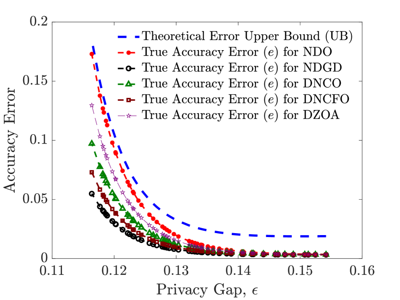
Figure 1: Theoretical accuracy error upper bound ($\textstyle{\mathrm{UB}}$) computed according to (30) in Theorem 2 with the perturbation slope $\tilde{m}^{*}$ obtained by solving the LP in 20, as well as true accuracy error $\|x^{*}-\tilde{x}^{*}\|_{\infty}$ for $50$ randomly sampled perturbations $\tilde{m}$ from the normal distribution $\mathcal{N}(\tilde{m}^{*},1)$ obtained by applying the nonconvex distributed optimization algorithms NDO [23], NDGD [24], DNCO [25], DNCFO [26] and DZOA [27].

VI Conclusion and Future Work

This paper introduced a novel notion of guaranteed privacy for a broad class of differentiable locally Lipschitz nonconvex distributed optimization problems. We showed how this property holds for a deterministic type of perturbation mechanisms, which exploit the Jacobian sign-stability of the problem objective functions. Furthermore, using robust optimization techniques, a tractable approach was provided to further restrict the mechanism in a way that allows for the quantification of the accuracy bounds of the method. In particular, these bounds were shown to be decreasing with respect to the privacy gap, as illustrated through simulations. Future work will consider utilizing the results in Theorem 1 to design privacy-preserving estimation, verification and resource/task allocation algorithms in networked CPS.

References

• [1] J. Cortés, G.E. Dullerud, S. Han, J. Le Ny, S. Mitra, and G.J. Pappas. Differential privacy in control and network systems. In 2016 IEEE 55th Conference on Decision and Control (CDC), pages 4252–4272. IEEE, 2016.
• [2] C. Dwork, F. McSherry, K. Nissim, and A. Smith. Calibrating noise to sensitivity in private data analysis. In Theory of cryptography conference, pages 265–284. Springer, 2006.
• [3] K. Chaudhuri, C. Monteleoni, and A.D. Sarwate. Differentially private empirical risk minimization. Journal of Machine Learning Research, 12(3), 2011.
• [4] J. Zhang, Z. Zhang, X. Xiao, Y. Yang, and M. Winslett. Functional mechanism: regression analysis under differential privacy. arXiv preprint arXiv:1208.0219, 2012.
• [5] R. Hall, A. Rinaldo, and L. Wasserman. Differential privacy for functions and functional data. The Journal of Machine Learning Research, 14(1):703–727, 2013.
• [6] Y. Wang, Z. Huang, S. Mitra, and G.E. Dullerud. Differential privacy in linear distributed control systems: Entropy minimizing mechanisms and performance tradeoffs. IEEE Transactions on Control of Network Systems, 4(1):118–130, 2017.
• [7] Y. Han and S. Martínez. A numerical verification framework for differential privacy in estimation. IEEE Control Systems Letters, 6:1712–1717, 2021.
• [8] Z. Huang, S. Mitra, and N. Vaidya. Differentially private distributed optimization. In Proceedings of the 2015 international conference on distributed computing and networking, pages 1–10, 2015.
• [9] S. Han, U. Topcu, and G.J. Pappas. Differentially private distributed constrained optimization. IEEE Transactions on Automatic Control, 62(1):50–64, 2016.
• [10] M.T. Hale and M. Egerstedty. Differentially private cloud-based multi-agent optimization with constraints. In 2015 American Control Conference (ACC), pages 1235–1240. IEEE, 2015.
• [11] T. Ding, S. Zhu, J. He, C. Chen, and X. Guan. Differentially private distributed optimization via state and direction perturbation in multiagent systems. IEEE Transactions on Automatic Control, 67(2):722–737, 2021.
• [12] Q. Li, R. Heusdens, and M.G. Christensen. Privacy-preserving distributed optimization via subspace perturbation: A general framework. IEEE Transactions on Signal Processing, 68:5983–5996, 2020.
• [13] M. Ye, G. Hu, L. Xie, and S. Xu. Differentially private distributed Nash equilibrium seeking for aggregative games. IEEE Transactions on Automatic Control, 67(5):2451–2458, 2021.
• [14] E. Nozari, P. Tallapragada, and J. Cortés. Differentially private distributed convex optimization via functional perturbation. IEEE Transactions on Control of Network Systems, 5(1):395–408, 2016.
• [15] Y. Wang, H. Sibai, M. Yen, S. Mitra, and Dullerud g.E. Differentially private algorithms for statistical verification of cyber-physical systems. http://128.84.4.18/pdf/2004.00275, 2022.
• [16] D. Bertsekas, A. Nedic, and A. Ozdaglar. Convex analysis and optimization, volume 1. Athena Scientific, 2003.
• [17] L. Jaulin, M. Kieffer, O. Didrit, and E. Walter. Applied interval analysis. ed: Springer, London, 2001.
• [18] M. Khajenejad and S.Z. Yong. Tight remainder-form decomposition functions with applications to constrained reachability and interval observer design. IEEE Transactions on Automatic Control, accepted, arXiv preprint arXiv:2103.08638, 2022.
• [19] L. Yang, O. Mickelin, and N. Ozay. On sufficient conditions for mixed monotonicity. IEEE Transactions on Automatic Control, 64(12):5080–5085, 2019.
• [20] M. Khajenejad, F. Shoaib, and S.Z. Yong. Guaranteed state estimation via indirect polytopic set computation for nonlinear discrete-time systems. In 2021 60th IEEE Conference on Decision and Control (CDC), pages 6167–6174. IEEE, 2021.
• [21] A. Ben-Tal, L. El Ghaoui, and A. Nemirovski. Robust optimization, volume 28. Princeton university press, 2009.
• [22] D. Efimov, T. Raïssi, S. Chebotarev, and A. Zolghadri. Interval state observer for nonlinear time varying systems. Automatica, 49(1):200–205, 2013.
• [23] T. Tatarenko and B. Touri. Non-convex distributed optimization. IEEE Transactions on Automatic Control, 62(8):3744–3757, 2017.
• [24] J. Zeng and W. Yin. On nonconvex decentralized gradient descent. IEEE Transactions on signal processing, 66(11):2834–2848, 2018.
• [25] G. Scutari and Y. Sun. Distributed nonconvex constrained optimization over time-varying digraphs. Mathematical Programming, 176(1):497–544, 2019.
• [26] H. Sun and M. Hong. Distributed non-convex first-order optimization and information processing: Lower complexity bounds and rate optimal algorithms. IEEE Transactions on Signal processing, 67(22):5912–5928, 2019.
• [27] Y. Tang, J. Zhang, and N. Li. Distributed zero-order algorithms for nonconvex multiagent optimization. IEEE Transactions on Control of Network Systems, 8(1):269–281, 2020.