Autocorrelation analysis for cryo-EM with sparsity constraints: Improved sample complexity and projection-based algorithms

Abstract.

The number of noisy images required for molecular reconstruction in single-particle cryo-electron microscopy (cryo-EM) is governed by the autocorrelations of the observed, randomly-oriented, noisy projection images. In this work, we consider the effect of imposing sparsity priors on the molecule. We use techniques from signal processing, optimization, and applied algebraic geometry to obtain new theoretical and computational contributions for this challenging non-linear inverse problem with sparsity constraints. We prove that molecular structures modeled as sums of Gaussians are uniquely determined by the second-order autocorrelation of their projection images, implying that the sample complexity is proportional to the square of the variance of the noise. This theory improves upon the non-sparse case, where the third-order autocorrelation is required for uniformly-oriented particle images and the sample complexity scales with the cube of the noise variance. Furthermore, we build a computational framework to reconstruct molecular structures which are sparse in the wavelet basis. This method combines the sparse representation for the molecule with projection-based techniques used for phase retrieval in X-ray crystallography.

Sparsity is a ubiquitous prior in many linear inverse problems, including regression [92, 43], compressed sensing [27, 19, 30], and various image processing applications [29], to name a few. While sparse priors are also used for non-linear inverse problems, their applicability and theoretical foundations are limited to a few specific (usually linear and quadratic) models, e.g., [17, 23, 33, 96]. Motivated by single-particle cryo-EM—an imaging technology for determining the 3-D structure of biological molecules—this paper uses modern techniques from signal processing, optimization, and applied algebraic geometry to provide new theoretical analysis and computational methods for a challenging non-linear inverse problem with sparsity constraints.

Cryo-EM has garnered increasing interest in the past decade due to a series of technological and algorithmic breakthroughs, driving a striking improvement in the obtainable resolution, up to the level where individual atoms can be distinguished. This has in turn opened new scientific horizons and led to many biological discoveries, e.g., [58, 3, 18].

In a cryo-EM experiment, a solution containing molecules to be imaged is rapidly frozen into a thin ice layer, which is then placed in an electron microscope. Next, the microscope acquires an image, called micrograph, which contains multiple 2-D tomographic projection images of the molecules. The 3-D orientations of individual projection images are unknown and random. To avoid damaging the samples, the electron dose must be kept low, resulting in a low signal-to-noise ratio (SNR). The cryo-EM computational problem is reconstructing the 3-D molecular structure from these projection images [38].

The renewed interest in cryo-EM led to a thorough investigation of its mathematical and statistical foundations [87, 6]. In particular, a crucial challenge from a statistical perspective is understanding the sample complexity of cryo-EM, i.e., the number of images that are required to obtain accurate reconstructions. A remarkable result revealed an intimate connection between the sample complexity of cryo-EM (and related statistical models) and the method of moments in the low SNR regime. If the distribution of the 3-D rotations is uniform, the method of moments reduces to autocorrelation analysis. In particular, it was shown that if $d$ is the lowest degree moment of the observations (i.e., the randomly oriented tomographic projections) that determines the molecular structure uniquely, a necessary condition for recovery is $n=\omega(\sigma^{2d}),$ namely, $n/\sigma^{2d}\to\infty$ as $n\to\infty$) where $\sigma^{2}$ is the variance of the noise [74, 1]. Specifically, if the distribution of rotations is uniform, then the third-order autocorrelation is the lowest order autocorrelation that determines a generic 3-D structure, implying a sample complexity of $n=\omega(\sigma^{6})$ [4]. This agrees with long-standing empirical evidence [86].

Autocorrelation analysis was first introduced to cryo-EM by Zvi Kam more than 40 years ago [52]. Kam showed that the second-order autocorrelation of the projection images (which can be estimated with $n=\omega(\sigma^{4})$ observations) determines the 3-D structure up to a set of orthogonal matrices, under the assumption that the rotations are drawn from a uniform distribution. A few methods have been proposed to resolve the missing orthogonal matrices based on typically unavailable side information, such as homologous models with known structure, or a few clean projections images, in order to construct ab initio models [14, 63, 48]. These ab initio models can then be refined using expectation-maximization: the prevalent algorithmic framework for the cryo-EM reconstruction problem that aims to maximize the non-convex posterior distribution [86, 81, 76]. In addition, it was recently shown that if the distribution of rotations is non-uniform, then there is at most a finite list of structures that agree with the second moment of the observations [83]. Techniques that are inspired by Kam’s method were also proposed as a solution to the molecular reconstruction problem in X-ray free-electron lasers (XFEL), which, akin to the reconstruction problem in cryo-EM, involves recovering a 3-D structure from its randomly oriented diffraction images [78, 59, 26, 60]. In contrast to cryo-EM, in XFEL the rotations are more likely to be uniformly distributed for particles with nearly uniform dimensions and the reconstruction problem is more involved since the measurements consist of the magnitudes of Fourier coefficients without their phases.

The first contribution of this paper is proving that if the sought-for molecular structure can be described as a sparse combination of Gaussian functions, then the structure can be determined uniquely from the second-order autocorrelation of the observations, even if the rotations are distributed uniformly. This eliminates the orthogonal matrix ambiguity in Kam’s original paper [52]. This result is the first theoretical guarantee for unique recovery from the second moment. It combines the sparsity assumption with proof techniques from real algebraic geometry, substantially reducing the sample complexity of the cryo-EM reconstruction problem from $n=\omega(\sigma^{6})$ to $n=\omega(\sigma^{4})$. The argument is constructive in the sense that it provides a polynomial-time recovery algorithm. However, the said algorithm is tailored to the specific model of point mass functions. It is not well-suited to data discretized into pixels or voxels because it hinges on the ability to cluster points in the support of the second moment into certain distinct components, see Remark 12. (Accurate clustering becomes difficult when data is discretized and the components are close to each other.)

The second contribution of this paper is a practical algorithm, fusing the second-order autocorrelation of the projections with a sparse representation of the molecular structure, and requiring only $n=\omega(\sigma^{4})$ observations. The algorithm builds on the realization that a typical 3-D structure can be represented by only a few coefficients in a suitable basis. Similar sparsity assumptions have been leveraged in a wide variety of scientific and engineering applications, including compressed sensing [27, 19, 30], image processing [29], and phase retrieval [17, 23, 49, 33, 96], to name a few. In cryo-EM, there have been several attempts to represent the 3-D structure as either a sparse mixture of Gaussians [95, 51, 50, 54, 97, 21, 77] or using alternative bases [94]. In particular, in settings with sufficiently high SNR where it is possible to identify the Gaussian mixtures within individual projection images, the inverse problem simplifies and can be solved [71, 72]. Yet, the sparsity property has still not been fully harnessed to represent and recover 3-D molecular structures, and it is not part of the standard computational pipeline of cryo-EM.

The technique is based on a new connection between Kam’s theory for cryo-EM and the crystallographic phase retrieval problem—recovering a sparse signal from its Fourier magnitudes. In particular, we adapt projection-based algorithms that were designed for the crystallographic phase retrieval problem to the cryo-EM setting. These algorithms were extensively validated on experimental X-ray crystallography datasets by prior researchers, see for example [36, 31, 64, 34, 33]. Here, we demonstrate on simulated data that they are also useful in constructing ab initio models in cryo-EM. They can be used to mitigate computational and model bias issues associated with the non-convexity of the cryo-EM reconstruction problem [89, 76, 45]. This new computational approach opens the door to merging more aspects of the phase retrieval and cryo-EM fields in future work.

The rest of the paper is organized as follows. In Section 1, we provide background on the reconstruction problem in cryo-EM, the method of moments, Kam’s theory, and the crystallographic phase retrieval problem. In Section 2, we prove that a structure composed of an ensemble of ideal point masses subject to uniform rotations can be recovered from the second order autocorrelation, implying a sample complexity of $n=\omega(\sigma^{4})$. Section 3 outlines the practical computational framework and presents numerical results. Section 4 concludes the paper and discusses potential theoretical and computational extensions.

1. Preliminaries

1.1. The cryo-EM problem

Cryo-EM reconstruction seeks to determine a 3-D molecular structure $\Phi$ from its 2-D noisy tomographic projections, taken at random viewing angles. In this work, we focus on the case of uniformly random rotations. Uniformity is often taken as a baseline model, was the setting in Kam’s paper [52], and is harder than the case of a non-uniform distribution of rotations in the sense that it requires asymptotically more images (without sparsity priors) [4, 83]. Formally, let $\mu$ be the Haar probability measure on the compact group $\operatorname{SO}(3)$ of 3-D rotations, representing the uniform distribution. Assuming that we observe i.i.d. 2-D images of $\Phi$ after it has been randomly rotated according to $\mu$ and then tomographically projected to the plane, each projection image is modeled as:

(1) $$I_{R}(x,y)=\int_{z=-\infty}^{\infty}(R\cdot\Phi)(x,y,z)dz\,+\,\varepsilon(x,y),\quad R\sim\mu,$$

where $\varepsilon(x,y)$ is white Gaussian noise with known variance $\sigma^{2}$, and $R\cdot\Phi$ denotes the action of the rotation $R$ on $\Phi$. Here, typically, the variance of the noise $\sigma^{2}$ is much greater than the magnitude of the clean projection.

The cryo-EM problem is to estimate the molecular structure $\Phi$ from $n$ realizations of (1), i.e., from the 2-D observations $I_{R_{1}},I_{R_{2}},\ldots,I_{R_{n}}$. In Section 4, we discuss how the proposed framework can be extended to account for additional aspects in the generative model for cryo-EM images.

1.2. The method of moments

Our theoretical and computational contributions are based on the method of moments—a basic statistical inference technique tracing back to the seminal paper of Karl Pearson in the end of the 19th century. Specifically, we use the second moment of the observations (1), and relate it to the sought-for 3-D structure.

The (debiased) second observable moment is given by

(2) $$\overline{M_{2}}((x_{1},y_{1}),(x_{2},y_{2}))=\frac{1}{n}\sum_{i=1}^{n}I_{R_{i}}(x_{1},y_{1})I_{R_{i}}(x_{2},y_{2})-B(\sigma^{2}),$$

where $B(\sigma^{2})$ is a bias term that depends only on the noise variance. For large enough $n$, we have

(3) $$\overline{M_{2}}((x_{1},y_{1}),(x_{2},y_{2})) \approx M_{2}((x_{1},y_{1}),(x_{2},y_{2})),$$

where

(4) $$M_{2}((x_{1},y_{1}),(x_{2},y_{2})):=\!\!\!\int_{\operatorname{SO}(3)}\!\!\!\!\!\!\!\!\!\!\!\!I_{R}(x_{1},y_{1})I_{R}(x_{2},y_{2})d\mu(R)-B(\sigma^{2}),$$

denotes the (debiased) population second moment, which is a function of $\Phi$ through Eq. (1). More precisely, for $n=\omega(\sigma^{4})$ it holds $\overline{M_{2}}=M_{2}+o(1)$ with high probability.

The idea of the method of moments is to find a structure $\Phi$ which matches the observable moments. It is an alternative to other standard statistical estimation methods, e.g., maximum likelihood estimation (MLE). That said, a recent paper suggests that in the low SNR regime, the method of moments approximates the MLE [53].

1.3. Kam’s method

We detail a specific approach to autocorrelation analysis in cryo-EM, introduced by Kam [52]. To this end, we need to introduce a convenient basis for representing a 3-D structure $\Phi$, the spherical Bessel basis [2]. An expansion of maximum degree $L$ is defined by first expanding the Fourier transform $\mathcal{F}(\Phi)$ of $\Phi$ in spherical harmonics as

(5) $$\mathcal{F}(\Phi)(k,\theta,\varphi)\approx\sum_{\ell=0}^{L}\sum_{m=-\ell}^{\ell}A_{\ell m}(k)Y^{m}_{\ell}(\theta,\varphi),$$

where $k$ denotes the radial frequency and $Y^{m}_{\ell}(\theta,\varphi)$ are the spherical harmonics. In addition, the spherical harmonics coefficients $A_{\ell m}(k)$ are expanded by spherical Bessel functions, up to degree $S_{\ell}$, as

(6) $$A_{\ell m}(k)\approx\sum_{s=1}^{S_{\ell}}a_{\ell ms}j_{\ell s}(k).$$

The functions $j_{\ell s}(k)$ are the normalized spherical Bessel functions. By allowing $L$ and $S_{\ell}$ to grow unboundedly, any bandlimited function with bandlimit 1 can be represented in this basis. However, when expanding 3-D molecular structures from discretized projection images, the Nyquist criterion applied to the projection images limits the amount of extractable information. This determines bounds on the maximally allowable truncation parameters $L$ and $S_{\ell}$; see the appendix for a detailed description.

We aim to recover the coefficients $a_{\ell ms}$ (up to rotation and reflection in $\mathbb{R}^{3}$). As will be shown next, it is convenient to gather the coefficients into matrices $A_{\ell}$, of size $S_{\ell}\times(2\ell+1)$, via $A_{\ell}(s,m):=a_{\ell ms}$, for each $\ell=0,\ldots,L$.

Provided that the distribution of viewing angles is uniform, Kam [52] showed that the second moment of the Fourier transform of the projection images yields estimates for the following $S_{\ell}\times S_{\ell}$ matrices:

(7) $$C_{\ell}(s_{1},s_{2}):=\sum_{m=-\ell}^{\ell}A_{\ell}(s_{1},m)\overline{A_{\ell}(s_{2},m)}=A_{\ell}A_{\ell}^{*}.$$

Applying the Cholesky decomposition to each $C_{\ell}$ in (7) and imposing $\Phi$ to be real-valued, knowledge of (7) identifies each matrix of coefficient $A_{\ell}$ up to an unknown real, orthogonal transformation, provided $S_{\ell}\geq 2\ell+1$. That is, we can compute $A_{\ell}O_{\ell}$ for some unknown orthogonal matrix $O_{\ell}$ in the group $O(2\ell+1)$. Therefore, the second moment determines $\Phi$ up to a set of orthogonal matrices. To recover these matrices, and thus the 3-D structure, additional information is required. In this paper, we suggest using a sparsity assumption.

1.4. Crystallographic phase retrieval

One of the contributions of this paper is to relate the cryo-EM reconstruction problem to crystallographic phase retrieval. Phase retrieval is the main computational challenge in X-ray crystallography, which is still a leading method for elucidating the atomic structure of molecules. The prevalence of crystallography is witnessed by the remarkable fact that 25 Nobel Prizes have been awarded for work directly or indirectly involving crystallography [40]. Although there exist additional important phase retrieval applications (see for example [84, 26, 7, 5]), X-ray crystallography is by far the most widely investigated application.

The crystallographic phase retrieval problem entails recovering a sparse signal $x$ from its periodic autocorrelation (or, equivalently, from its Fourier transform magnitudes, namely, its power spectrum). While simply stated, and despite its importance, the theoretical foundations of this problem continue to evolve. In particular, it was recently conjectured that a generic sparse signal can be recovered from its periodic autocorrelation if the number of non-zero entries is smaller than half the signal’s length [9]. This conjecture was verified for a few cases. The relation of the crystallographic phase retrieval problem with the beltway problem from combinatorial optimization is explored in [41]. Our theoretical reconstruction guarantees in the following section can be viewed as analogous results in the setting of cryo-EM.

The standard algorithms for crystallographic phase retrieval build on two projection operators: one onto the measured data (the power spectrum) and the second onto the space of sparse signals. While simple algorithms that alternate between these two projections tend to quickly stagnate, a more sophisticated family of algorithms, based on reflections, shows excellent performance, though their running time is exponential in the sparsity level [33, 13]. These algorithms are tightly related to splitting methods, such as Douglas-Rachford and the alternating direction method of multipliers (ADMM), and have been applied to a wide variety of problems [34]. A main contribution of this paper is a modification of these algorithms to autocorrelation analysis for cryo-EM. In particular, we focus on one such algorithm, called relaxed-reflect-reflect (RRR), but alternative algorithms, such as Fienup’s hybrid input-output algorithm [36], the difference map algorithm [31], and the relaxed averaged alternating reflections algorithm [64], can be adapted to cryo-EM by the same strategy. Importantly, if the model is accurate (e.g., no noise and the correct sparsity level is known) RRR iterations halt only when they find a solution that satisfies both constraints (defined by the projection operators). Thus, RRR does not suffer from local minima as gradient-based algorithms do.

2. Superior sample complexity: The second moment suffices for sums of point masses

This section presents our main theoretical result: the second moment suffices to recover an idealized sparse volume, i.e., a volume given as a weighted sum of point masses. We deduce that the second moment also suffices for a pixelated and blurred variant of the model. Our theorems imply an associated sample complexity of $n=\omega(\sigma^{4})$. This stands in contrast to previous results which do not assume sparsity. There, the third moment is required for recovery, and the associated sample complexity is $n=\omega(\sigma^{6})$ [4, 35].

2.1. Models and main theoretical results

We use an atomistic representation of a molecule. In our first idealized model, an atom is specified by a weighted Dirac delta function, and a molecule is a sum of such point masses. In more detail, let $\mathbf{a}_{1},\ldots,\mathbf{a}_{p}\in\mathbb{R}^{3}$ be the 3-D points representing atom locations, and $w_{1},\ldots,w_{p}$ be positive weights corresponding to the scattering potentials of the individual atoms. Then,

(8) $$\Phi:=\sum_{i=1}^{p}w_{i}\delta_{\mathbf{a}_{i}},$$

is the molecule composed of the atoms $(\mathbf{a}_{i},w_{i})$. Relabeling if necessary, we assume that the $\ell^{2}$-norms $\|\mathbf{a}_{i}\|$ are in descending order.

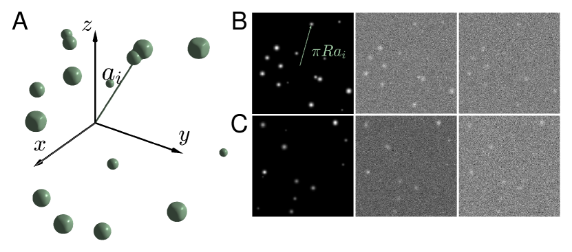
Figure 1. (A) Example of a structure of the form in (8). For this illustration, the size of each dot is proportional to the weight $w_{i}$. (B–C) Two examples of tomographic projections of rotated versions of (A), with no noise (leftmost), signal-to-noise ratio 0.04 (middle) and signal-to-noise ratio 0.01 (rightmost).

We model each projection image $I_{R}$ as a mixture of $p$ Dirac delta functions on $\mathbb{R}^{2}$ plus noise:

(9) $$I_{R}(x,y):=\sum_{i=1}^{p}w_{i}\delta_{\pi R\mathbf{a}_{i}}(x,y)+\varepsilon(x,y).$$

Here $\pi:\mathbb{R}^{3}\rightarrow\mathbb{R}^{2}$ denotes coordinate projection onto the first two coordinates, and $\varepsilon$ is white Gaussian noise with (known) variance $\sigma^{2}$. Given $n$ 2-D images as in (9), the reconstruction problem is to recover the atoms $(\mathbf{a}_{i},w_{i})$ in (8) up to a global rotation and reflection. (The reflection ambiguity exists because a molecule and its reflection in the microscope’s image plane are indistinguishable given cryo-EM data, see e.g. [38].) See Fig. 1 for an illustration of the setup.

Under this model the (debiased) second population moment, obtained by substituting (9) into (4), reads:

(10) $$\begin{split}&M_{2}((x_{1},y_{1}),(x_{2},y_{2}))=\sum_{i=1}^{p}\sum_{j=1}^{p}w_{i}w_{j}\,\times\\ &\qquad\qquad\qquad\quad\int_{\operatorname{SO}(3)}\!\!\!\!\delta_{\pi R\mathbf{a}_{i}}(x_{1},y_{1})\delta_{\pi R\mathbf{a}_{j}}(x_{2},y_{2})d\mu(R),\end{split}$$

where $\mu$ is the uniform distribution. Note that $M_{2}$ is a measure on $\mathbb{R}^{2}\!\times\mathbb{R}^{2}$.

We introduce two assumptions on the atom locations:

1. The vectors $\mathbf{a}_{i}$ are pairwise linearly independent;

2. The norms $\|\mathbf{a}_{i}\|$ are distinct.

We remark that conditions A1 and A2 are quite restrictive, e.g., ruling out molecules with nontrivial point-group symmetries.

Our first main theoretical result is stated as follows.

Theorem 1.

Consider the model given by (8)-(9). Assume that conditions A1-A2 hold. Then, the support of the second moment $M_{2}$ uniquely determines the set of triples $\{(\|\mathbf{a}_{i}\|^{2},\|\mathbf{a}_{j}\|^{2},\langle\mathbf{a}_{i},\mathbf{a}_{j}\rangle):i,j=1,\ldots,p\}$. Therefore, $M_{2}$ (Eq. (10)) uniquely determines the set of atom locations $\{\mathbf{a}_{i}:i=1,\ldots,p\}$ up to a rotation and reflection in $\mathbb{R}^{3}$.

Theorem 1 is proven in Subsection 2.3, after auxiliary results are given in Subsection 2.2.

Building on the uniqueness in Theorem 1, we obtain the following constructive result as well.

Theorem 2.

Consider the model given by (8)-(9). Assume that $p\geq 3$ and conditions A1-A2 hold. Then, Algorithm 1 (described in Subsection 2.4) recovers the set of atoms $\{(\mathbf{a}_{i},w_{i}):i=1,\ldots,p\}$ up to a rotation and reflection of the atom locations in $\mathbb{R}^{3}$ from the second moment $M_{2}$ (Eq. (10)) in $\mathcal{O}(p^{2})$ flops.

Theorem 2 is proven in Subsection 2.4. In fact the model of (8)-(9) can be extended to Gaussians of non-zero width of the form

(11) $$\Phi(\mathbf{x}):=\sum_{i=1}^{p}w_{i}k(\mathbf{x}-\mathbf{a}_{i}),$$

where $k(\mathbf{x})=e^{-\frac{\|\mathbf{x}\|^{2}}{2\kappa^{2}}}$ is an isotropic Gaussian with standard deviation $\kappa>0$. Our results guarantee unique recovery from the second moment also for this model. The proof of the following result is given in the appendix.

Theorem 3.

Consider the model given by (11). Assume that conditions A1-A2 hold. Then the second moment $M_{2}^{G}$ of the projection images formed from the model in (11) uniquely determines the set of atom locations and weights $\{(w_{i},\mathbf{a}_{i}):i=1,\ldots,p\}$ up to a joint rotation and reflection of the atom locations in $\mathbb{R}^{3}$.

We next discuss an additional extension of the model of (8)-(9). Prior works on the sample complexity of cryo-EM [4, 73, 1] do not directly apply to the models above. The principal reason is that the measurement formation defined by (9) is not finite-dimensional. Therefore, we consider a pixelated and blurred variant of the model. The molecule is still specified by a collection of atoms $\{(\mathbf{a}_{i},w_{i}):i=1,\ldots,p\}$. However, each projection image now consists of $2^{m}\!\times 2^{m}$ pixels:

(12) $$I_{R}^{[m]}(j_{1},j_{2}):=\!\int_{j_{2}\tau}^{(j_{2}+1)\tau}\!\!\!\int_{j_{1}\tau}^{(j_{1}+1)\tau}\!\!\!\left(\sum_{i=1}^{p}w_{i}\delta_{\pi R\mathbf{a}_{i}}(x,y)\right)\\ \ast k(x,y)dxdy+\varepsilon(j_{1},j_{2}).$$

Here, we discretized $[-1,1]^{2}$ into equi-sized squares, where $j_{1},j_{2}\in\{-2^{m-1},-2^{m-1}+1,\ldots,2^{m-1}-1\}$ and $\tau=1/2^{m-1}$. Also, $\ast$ denotes convolution and $k(x,y)$ is the isotropic Gaussian kernel with fixed variance $\kappa^{2}$, i.e., $k(x,y)=e^{\frac{-x^{2}-y^{2}}{2\kappa^{2}}}$. Last, the noise satisfies $\varepsilon(j_{1},j_{2})\overset{i.i.d.}{\sim}\mathcal{N}(0,\sigma^{2})$.

In the pixelated model, the (debiased) second population moment equals:

(13) $$M_{2}^{[m]}((j_{1},j_{2}),(j_{3},j_{4}))=\int_{j_{4}\tau}^{(j_{4}+1)\tau}\!\int_{j_{3}\tau}^{(j_{3}+1)\tau}\!\int_{j_{2}\tau}^{(j_{2}+1)\tau}\!\int_{j_{1}\tau}^{(j_{1}+1)\tau}\\ M_{2}((x_{1},y_{1}),(x_{2},y_{2}))\!\ast\!\left(k(x_{1},y_{1})k(x_{2},y_{2})\right)dx_{1}dy_{1}dx_{2}dy_{2}.$$

We now state our main result for the pixelated model. Its proof relies on Theorems 1 and 2.

Theorem 4.

Consider the model given by (12). Fix an integer $p\geq 3$ and real numbers $r>0$ and $w_{+}>w_{-}>0$. Assume that A1-A2 hold, and for each $i=1,\ldots,p$ we have $\|\mathbf{a}_{i}\|\leq r$ and $w_{-}\leq w_{i}\leq w_{+}$. Then, there exists $m^{\prime}=m^{\prime}(p,r,w_{+},w_{-})$ with the following property. Whenever $m\geq m^{\prime}$ and $2^{m}\times 2^{m}$ pixels are used in (12), then the second moment $M_{2}^{[m]}$ (Eq. (13)) uniquely determines the set of atoms $\{(\mathbf{a}_{i},w_{i}):i=1,\ldots,p\}$ up to a rotation and reflection in $\mathbb{R}^{3}$.

As the details are technical, we prove Theorem 4 in the appendix. We only use two properties of the Gaussian kernel $k$: that it is real-analytic and that its Fourier transform does not vanish.

Corollary 5.

Assume the setting of Theorem 4 with $m\geq m^{\prime}$. Then, the sample complexity for generic unique recovery (in the sense of [4]) is $n=\omega(\sigma^{4})$ as $\sigma\rightarrow\infty$.

The rest of the section provides the proofs of Theorems 1 and 2, with Theorem 4, Corollary 5 and supporting results shown in the appendix. We emphasize that Algorithm 1 is a theoretical algorithm, not intended for use in practice due to its noise sensitivity as explained in Remark 12. By contrast, Algorithm 2 in the subsequent section is built for practical situations.

2.2. Support of $M_{2}$

To recover the atoms from $M_{2}$, the main information that we use is actually qualitative. Specifically, we rely on the particular structure of the support of the second moment $M_{2}$ in $\mathbb{R}^{2}\times\mathbb{R}^{2}$. To describe this, we need to first understand the possible images of one pair of atoms.

Definition 6.

For $i,j=1,\ldots,p$, let $\theta_{ij}:\operatorname{SO}(3)\rightarrow\mathbb{R}^{2}\times\mathbb{R}^{2}$ be the map given by $\theta_{ij}(R)=(\pi R\mathbf{a}_{i},\pi R\mathbf{a}_{j})$.

Definition 7.

For $i,j=1,\ldots,p$, let $S_{ij}\subseteq\mathbb{R}^{2}\times\mathbb{R}^{2}$ be the image of $\theta_{ij}$, i.e., $S_{ij}=\{(\mathbf{x}_{1},\mathbf{x}_{2})\in\mathbb{R}^{2}\times\mathbb{R}^{2}:\exists R\in\operatorname{SO}(3)\textup{ s.t. }\pi R\mathbf{a}_{i}=\mathbf{x}_{1},\pi R\mathbf{a}_{j}=\mathbf{x}_{2}\}$.

The next lemma characterizes $S_{ij}\subseteq\mathbb{R}^{2}\times\mathbb{R}^{2}$ as the solution set to a system of polynomial equations and inequalities. This will enable proof techniques from real algebraic geometry.

Lemma 8.

Assume $i\neq j$. Then the set $S_{ij}$ is connected, compact and semialgebraic. Letting $((x_{1},y_{1}),(x_{2},y_{2}))$ be variables on $\mathbb{R}^{2}\times\mathbb{R}^{2}$, $S_{ij}$ is cut out by one quartic equation and two quadratic inequalities:

$$\left(\|\mathbf{a}_{i}\|^{2}\!-x_{1}^{2}\!-y_{1}^{2}\right)\!\!\left(\|\mathbf{a}_{j}\|^{2}\!-x_{2}^{2}\!-y_{2}^{2}\right)\!=\!\left(\langle\mathbf{a}_{i},\mathbf{a}_{j}\rangle\!-x_{1}x_{2}\!-y_{1}y_{2}\right)^{2}\!\!,$$

(14) $$\,x_{1}^{2}+y_{1}^{2}\leq\|\mathbf{a}_{i}\|^{2}\quad\quad\quad\text{and}\quad\quad\quad x_{2}^{2}+y_{2}^{2}\leq\|\mathbf{a}_{j}\|^{2}.$$

It has dimension $3$ as a semialgebraic set if condition A1 holds.

A few different examples of the sets $S_{ij}$ are illustrated in Fig. 2, for varying values of $\langle\mathbf{a}_{i},\mathbf{a}_{j}\rangle$ and $\|\mathbf{a}_{i}\|,\|\mathbf{a}_{j}\|$. There we show the projection of $S_{ij}$ to $\mathbb{R}^{3}$ when $y_{2}$ is dropped.

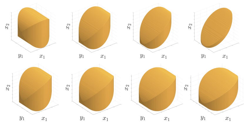
Figure 2. Illustration of the semialgebraic sets $S_{ij}$ described in Lemma 8, projected onto $(x_{1},y_{1},x_{2})$-space. Upper row from left to right: $\|\mathbf{a}_{i}\|=\|\mathbf{a}_{j}\|=1$ and $\langle\mathbf{a}_{i},\mathbf{a}_{j}\rangle=\cos{\frac{\pi}{2}},\cos{\frac{\pi}{4}},\cos{\frac{\pi}{6}},\cos{\frac{\pi}{20}}$, respectively. Lower row from left to right: $\langle\mathbf{a}_{i},\mathbf{a}_{j}\rangle=\|\mathbf{a}_{j}\|\cos{\frac{\pi}{3}}$, $\|\mathbf{a}_{i}\|=1$ and $\|\mathbf{a}_{j}\|=1,0.9,0.8,0.7$, respectively. By Lemma 9, these sets make up the support of $M_{2}$, which is the basis of our theory.

The next result is immediate from Definitions 6 and 7.

Lemma 9.

The second moment is

(15) $$M_{2}=\sum_{i,j=1}^{k}w_{i}w_{j}(\theta_{ij})_{*}(\mu),$$

where the subscripts indicate the pushforward measure defined by $(\theta_{ij})_{*}(\mu)(\cdot)=\mu\left(\theta_{ij}^{-1}(\cdot)\right)$. In particular, the support of $M_{2}$ is $\cup_{i,j=1}^{p}S_{ij}$.

2.3. Information-theoretic uniqueness: Proof of Theorem 1

We begin by proving Theorem 1. The key is a converse to Lemma 8. While Lemma 8 implies the quartic equation in (8) (plus the quadratic inequalities there) determine the set $S_{ij}$, we need that $S_{ij}$ determines the quartic. The proof of this converse uses results from real algebraic geometry [16].

Lemma 10.

Assume that condition A1 holds. Let $i\neq j$. Then, the ideal of the real Zariski closure of $S_{ij}$ in $\mathbb{R}^{2}\times\mathbb{R}^{2}$ is principal and generated by the quartic polynomial $q_{ij}$:

$$\left(\|\mathbf{a}_{i}\|^{2}\!-x_{1}^{2}\!-y_{1}^{2}\right)\!\!\left(\|\mathbf{a}_{j}\|^{2}\!-x_{2}^{2}\!-y_{2}^{2}\right)-\left(\langle\mathbf{a}_{i},\mathbf{a}_{j}\rangle\!-x_{1}x_{2}\!-y_{1}y_{2}\right)^{2}\!\!$$

$$=\left(\|\mathbf{a}_{i}\|^{2}\|\mathbf{a}_{j}\|^{2}-\langle\mathbf{a}_{i},\mathbf{a}_{j}\rangle^{2}\right)-\|\mathbf{a}_{j}\|^{2}x_{1}^{2}-\|\mathbf{a}_{j}\|^{2}y_{1}^{2}$$

$$\hskip 8.00003pt-\|\mathbf{a}_{i}\|^{2}x_{2}^{2}-\|\mathbf{a}_{i}\|^{2}y_{2}^{2}+2\langle\mathbf{a}_{i},\mathbf{a}_{j}\rangle x_{1}x_{2}+2\langle\mathbf{a}_{i},\mathbf{a}_{j}\rangle y_{1}y_{2}$$

(16) $$\hskip 8.00003pt+x_{1}^{2}y_{2}^{2}+y_{1}^{2}x_{2}^{2}-2x_{1}y_{1}x_{2}y_{2}.$$

Further, $q_{ij}$ is irreducible over $\mathbb{R}$.

Corollary 11.

Assume that conditions A1-A2 hold. Then, the irredundant irreducible decomposition of the Zariski closure of the support of $M_{2}$ is

(17) $$\{(\mathbf{x}_{1},\mathbf{x}_{2}):\mathbf{x}_{1}=\mathbf{x}_{2}\}\,\,\cup\,\,\bigcup_{i\neq j}\overline{S_{ij}}.$$

We can now prove the information-theoretic uniqueness.

Proof of Theorem 1.

The support of $M_{2}$ determines the real radical prime ideal of each of top-dimensional irreducible component of its Zariski closure. By A1-A2, Corollary 11 and Lemma 10, these ideals are $\langle q_{ij}\rangle=\{q_{ij}h\!:h\in\mathbb{R}[x_{1},y_{1},x_{2},y_{2}]\}$ for $i\neq j$. The ideal $\langle q_{ij}\rangle$ uniquely determines $q_{ij}$, since the coefficient of $x_{1}^{2}y_{2}^{2}$ in (10) is $1$. Extracting the coefficients of $x_{2}^{2},x_{1}^{2},x_{1}x_{2}$ in (10), $q_{ij}$ determines the triple $(\|\mathbf{a}_{i}\|^{2},\|\mathbf{a}_{j}\|^{2},\langle\mathbf{a}_{i},\mathbf{a}_{j}\rangle)$. Ranging over $i,j$, we have proven that the support of $M_{2}$ fixes the set:

(18) $$\{(\|\mathbf{a}_{i}\|^{2},\|\mathbf{a}_{j}\|^{2},\langle\mathbf{a}_{i},\mathbf{a}_{j}\rangle):i\neq j\}.$$

By A2 and our assumption that the norms $\|\mathbf{a}_{i}\|$ are descending, knowledge of (18) lets us fill in the Gram matrix:

(19) $$G\,=\,A^{\top}A\,\in\,\mathbb{R}^{p\times p},$$

where

(20) $$A\,=\,\begin{pmatrix}\mathbf{a}_{1}&\ldots&\mathbf{a}_{p}\end{pmatrix}\,\in\,\mathbb{R}^{3\times p}.$$

However $G$ determines $A$ up to left multiplication by a $3\times 3$ orthogonal matrix. Indeed considering a truncated rank-3 eigendecomposition, we write

(21) $$G=QDQ^{\top}\!,$$

where $Q\in\mathbb{R}^{p\times 3}$ has orthonormal columns and $D\in\mathbb{R}^{3\times 3}$ is diagonal and positive-semidefinite. Then,

(22) $$A=OD^{1/2}Q^{\top}\!,$$

for some $O\in\operatorname{O}(3)$. Therefore, the atoms’ locations $\mathbf{a}_{i}$ are determined up to a global rotation and reflection. ∎

2.4. Recovery algorithm: Proof of Theorem 2

Now, we move forward and prove Theorem 2. We present Algorithm 1 for efficiently recovering the atoms $(\mathbf{a}_{i},w_{i})$ from $M_{2}$. The algorithm is theoretical in that it relies on oracle access to the following information.

Assumption 1.

We assume oracle access to:

• $\{sample(S_{ij}):i\neq j\}$, where $sample(S_{ij})$ consists of four or more Zariski-generic points on $S_{ij}$;

• the value of the measure $M_{2}$ on the set $S_{ij}$ for all $i\neq j$.

Remark 12.

In principle, O1 and O2 could be estimated from the sample moment $\overline{M_{2}}$ (2) if $n=\omega(\sigma^{4})$. It would require the ability to identify points in the support of $M_{2}$ and cluster them according to the components $S_{ij}$. However this encounters difficulty when dealing with noisy moments discretized in pixels. The next section is dedicated to a different computational framework, which is suited for practical settings.

Proceeding, Algorithm 1 interpolates $sample({S_{ij}})$ to recover $q_{ij}$ from Lemma 10 (Eq. (10)).

Lemma 13.

Assume that condition A1 holds, and O1 is known. Let $sample({S_{ij}})=\{\left((x_{1k},y_{1k}),(x_{2k},y_{2k})\right):k=1,\ldots,|sample(S_{ij})|\}$. Consider the matrix

(23) $$\begin{pmatrix}&&1&&\\[1.99997pt] &&x_{1k}^{2}+y_{1k}^{2}&&\\[1.99997pt] &\ldots&x_{2k}^{2}+y_{2k}^{2}&\ldots&\\[1.99997pt] &&x_{1k}x_{2k}+y_{1k}y_{2k}&&\\[1.99997pt] &&x_{1k}^{2}y_{2k}^{2}+y_{1k}^{2}x_{2k}^{2}-2x_{1k}y_{1k}x_{2k}y_{2k}&&\end{pmatrix}^{\!\!\!\top}\!.$$

Then it has rank $4$, with kernel spanned by

(24) $$\begin{pmatrix}\|\mathbf{a}_{i}\|^{2}\|\mathbf{a}_{j}\|^{2}-\langle\mathbf{a}_{i},\mathbf{a}_{j}\rangle^{2}\\[1.99997pt] -\|\mathbf{a}_{j}\|^{2}\\[1.99997pt] -\|\mathbf{a}_{i}\|^{2}\\[1.99997pt] 2\langle\mathbf{a}_{i},\mathbf{a}_{j}\rangle\\[1.99997pt] 1\end{pmatrix}.$$

By Lemma 13, we compute the triples $\{(\|\mathbf{a}_{i}\|^{2},\|\mathbf{a}_{j}\|^{2},\langle\mathbf{a}_{i},\mathbf{a}_{j}\rangle):i\neq j\}$ in $\mathcal{O}(p^{2})$ time, by forming the matrices in Eq. (23) and computing their kernels. We then fill in the Gram matrix in Eq. (19) as in the proof of Theorem 1. The atoms’ locations $\mathbf{a}_{i}$ are recovered from the truncated eigendecomposition as in Eq. (22).

The calculation of the weights $w_{i}$ is based on the following.

Lemma 14.

Assume that conditions A1-A2 hold. Then, for each $i\neq j$, the measure of $S_{ij}$ with respect to $M_{2}$ is

(25) $$M_{2}(S_{ij})=w_{i}w_{j}.$$

Therefore, O2 tells us all off-diagonal entries of $ww^{\!\top}\!\in\mathbb{R}^{p\times p}$. We complete this uniquely to a rank-$1$ matrix by using

(26) $$(ww^{\!\top})_{ii}\,=\,\frac{(ww^{\!\top})_{ij^{\prime}}(ww^{\!\top})_{ji}}{(ww^{\!\top})_{jj^{\prime}}},$$

where $j,j^{\prime}$ are any indices such that $i,j,j^{\prime}$ are all distinct. (This step requires $p\geq 3$.) The weights $w_{i}$ are lastly recovered either by computing the leading eigenvector/eigenvalue pair of $ww^{\top}$ or as the square root of the diagonal of $ww^{\top}$, using the fact that the $w$ are non-negative.

Remark 15.

We note that (26) is a particular case of the problem of recovering a low-rank matrix with corrupted diagonal entries; see, e.g.,  [70, 79, 80] for more on that problem.

We summarize the procedure of this section in Algorithm 1.

Second population moment $M_{2}$ as in (10)

Atoms $\{(\mathbf{a}_{i},w_{i}):i=1,\ldots,p\}$ up to a rotation and reflection in $\mathbb{R}^{3}$

1. Access O1 in Assumption 1

2. Recover the unordered set $\{(\|\mathbf{a}_{i}\|^{2},\|\mathbf{a}_{j}\|^{2},\langle\mathbf{a}_{i},\mathbf{a}_{j}\rangle):i\neq j\}$ using Lemma 13

3. Fill in the Gram matrix $G=A^{\!\top}A$ with $A$ from (20)

4. Recover the $\mathbf{a}_{i}$ up to orthogonal transformation by computing a truncated eigendecomposition of $G$ as in (22)

5. Access O2 in Assumption 1

6. Fill in the off-diagonal entries of $ww^{\!\top}$ using Lemma 14

7. Complete $ww^{\!\top}$ using (26)

8. Recover the $w_{i}$ from $ww^{\!\top}$

return $\{(\mathbf{a}_{i},w_{i}):i=1,\ldots,k\}$

Algorithm 1 Recovering a sparse structure from its second moment

Proof of Theorem 2.

The considerations above show that Algorithm 1 correctly recovers the set of atoms $\{(\mathbf{a}_{i},w_{i}):i=1,\ldots,p\}$ from $M_{2}$ (up to a rotation and reflection in $\mathbb{R}^{3}$). It costs $\mathcal{O}(p^{2})$ in flops and storage once O1 and O2 are available if we use a randomized algorithm [69] to compute the truncated decomposition in (21). ∎

3. Kam’s method with sparsity constraints

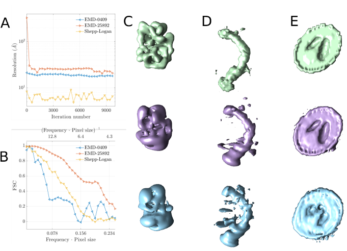
Figure 3. Reconstruction results when applying the proposed algorithm to three example structures. (A) Resolution of the reconstructed volumes as a function of the number of iterations. The resolution is determined by the $0.5$ cutoff of the Fourier Shell Correlation (FSC). (B) Example FSC curves for reconstructed volumes as function of non-dimensionalized frequency. (C,D,E) Visualization of the reconstructed volumes for the three example structures: EMD-0409 [46], EMD-25892 [65] and the Shepp-Logan phantom [85], respectively. (Top) Ground-truth structure. (Middle) Truncation of ground-truth structure into the spherical Bessel basis using $L=8,12,12$, respectively. (Bottom) Reconstructed volume returned by Alg. 2 using $L=8,12,12$, respectively. The visualizations were rendered by UCSF Chimera [75].

This section introduces a computational framework to leverage sparsity in recovering the underlying molecular structure. The goal is to devise a principled way to compute ab initio approximations of the underlying structures, that can then be improved further in a refinement step (which is typically performed using expectation-maximization [81, 76] or used for model validation. In this section, we maintain the assumption that the distribution $\mu$ of viewing angles is uniformly distributed. If $\mu$ is a non-uniform distribution, it is known that there is at most a finite list of structures that are consistent with the observed second order moment [83]; employing sparsity to aid in the recovery problem with non-uniform distribution will be considered in future work.

We use projection-based optimization techniques from the related problem of crystallographic phase retrieval, coupled with information extracted from the second moment of the projection images. Without imposing the underlying sparsity, the second moment of the projection images determines the structure up to an ambiguity encoded by a set of unknown orthogonal matrices. The key idea of the algorithm is to alternatingly project the molecular structure onto constraints encoded by the sparsity and by the projection image moments, respectively.

Analogously to (10), the moments of the projection images furnish information about the underlying 3-D structure. Unlike our theoretical results, however, we consider a general 3-D structure $\Phi$ expanded in a spherical Bessel basis as in Section 1.3. As in the previous section, Gaussians (and mixtures of a small number of Gaussians) are often used as first approximation to the scattering potential of individual atoms. These Gaussians have the majority of their energy concentrated in a region of finite support. They can therefore be approximated by a small number of localized basis functions, such as the Haar wavelets. The sparse mixtures of Gaussians from the preceding sections can therefore be viewed as having a sparse representation in a wavelet basis, which offers computational advantages. This section therefore assumes that $\Phi$ can be represented by only a few wavelet coefficients. We also mention that recent work appearing after this paper was submitted shows that, for almost any basis, the second moment determines the structure uniquely, if the structure is sparse when expanded in the basis [11]. The next section introduces wavelet bases, and later we provide the details of the projection-based algorithm.

3.1. Wavelet bases

We encode sparsity of a 3-D molecular structure $\Phi$ by a sparse expansion in wavelets [24]—a popular choice of sparsifying, localized bases in a wide range of applications [66]. Our algorithm can easily be adapted to any specific wavelet basis, and, more generally, to any choice of basis, for instance, sparsifying bases learned through data.

We denote the multilevel wavelet basis by $f_{m,n}$, where $m=1,\ldots,m_{\text{max}}$ denotes the level of the wavelet and $n=1,\ldots,n_{\text{max}}(m)$ the index of the function within the level. As a shorthand, we define $W:\mathbb{R}^{M\times M\times M}\rightarrow\mathbb{R}^{m_{\text{max}}n_{\text{max}}(m)}$ as the map sending a 3-D structure to its vector of coefficients when expanded in the wavelet basis, i.e.,

(27) $$W(\Phi)=\left(\langle\Phi,f_{m,n}\rangle\right)_{m,n=1}^{m_{\text{max}},n_{\text{max}}(m)}.$$

Likewise, $W^{-1}:\mathbb{R}^{m_{\text{max}}n_{\text{max}}(m)}\rightarrow\mathbb{R}^{M\times M\times M}$ then maps a wavelet coefficient vector into its 3-D expansion by

(28) $$W^{-1}\left(\left(c_{m,n}\right)_{m,n=1}^{m_{\text{max}},n_{\text{max}}(m)}\right)=\sum_{m,n}c_{m,n}f_{m,n}.$$

An additional advantage of using wavelet bases is that $W$ and $W^{-1}$ can then be applied in linear time $\mathcal{O}(M^{3})$ using a fast wavelet transform [67].

3.2. Projection-based algorithm

For a discretized 3-D structure $\Phi$ of size $M\times M\times M$, we define the mapping $\mathcal{SB}:\mathbb{R}^{M\times M\times M}\rightarrow\prod_{\ell=0}^{L}\mathbb{C}^{S_{\ell}\times(2\ell+1)}$ of the structure into its coordinates in the spherical Bessel basis by

(29) $$\mathcal{SB}(\Phi)=\left(A_{0},A_{1},\ldots,A_{L}\right).$$

The inverse mapping $\mathcal{SB}^{-1}:\prod_{\ell=0}^{L}\mathbb{C}^{S_{\ell}\times(2\ell+1)}\rightarrow\mathbb{R}^{M\times M\times M}$ then expands a set of coefficients in the spherical Bessel basis into its corresponding 3-D structure:

(30) $$\mathcal{SB}^{-1}\left(A_{0},\ldots,A_{L}\right)=\mathcal{F}^{-1}\left(\sum_{\ell,m,s}\!a_{\ell ms}j_{\ell s}(k)Y^{m}_{\ell}(\theta,\varphi)\!\right).$$

As discussed in Section 1, Kam’s method identifies matrices $A_{\ell}O_{\ell}$, for $O_{\ell}$ an unknown orthogonal matrix, for each $\ell$ with $S_{\ell}\geq 2\ell+1$. By possibly reducing the value of $L$ to the largest index with this property, we will for ease of notation assume that this property holds for $\ell=0,\ldots,L$. Therefore, at the onset of the algorithm, we have access to a set of coefficient matrices $B=(B_{0},\ldots,B_{L})$ satisfying

(31) $$B_{\ell}=A_{\ell}O_{\ell},\quad O_{\ell}\in O(2\ell+1),$$

for unknown orthogonal matrices $O_{\ell}$. Our algorithm aims to recover an approximation of these unknown orthogonal matrices, which leads to an approximation of $\Phi$. This orthogonal matrix retrieval problem is an analogue to the problem of the missing phases in the phase retrieval problem [10]. We therefore adapt a popular algorithm from the phase retrieval literature into the problem of cryo-EM. The algorithm repeatedly utilizes two projections onto the set of structures with a given sparsity level and a set determined by the projection images. These two projections are the main pillars of the algorithm and can be used in different ways, as explained next. But first, we define the two projection operators.

3.2.1. First projection: Moment constraint.

We begin by defining the first projection operator, denoted by $\rho_{1}$, as the projection onto the set defined by the $C_{\ell}$ matrices in (7). Let $\mathcal{SB}(\Phi)=(A_{0},\ldots,A_{L})$ in $\prod_{\ell=0}^{L}\mathbb{C}^{S_{\ell}\times(2\ell+1)}$ be the ordered collection of matrices of coefficients in the spherical Bessel basis. Define $\rho_{1}(\Phi)$ as the projection

(32) $$\rho_{1}(\Phi)=\mathcal{SB}^{-1}\left(D_{0},\ldots,D_{L}\right),$$

where the matrices $D_{\ell}$ are defined by

(33) $$\!\!(D_{0},\ldots,D_{L})\!=\!\!\operatorname*{argmin\,}_{(D_{0},\ldots,D_{L})}\!\!\!\!\left\{\|A_{\ell}\!-\!D_{\ell}\|_{\text{F}}:D_{\ell}D_{\ell}^{*}=C_{\ell}\right\},$$

with $C_{\ell}$ from (7). (33) is an instance of the Orthogonal Procrustes problem. Although it is a non-convex optimization problem, it can be solved in closed form in terms of the singular value decomposition of $B_{\ell}^{T}A_{\ell}$, see e.g., [82]. In the implementation, the matrices defining the operations $\mathcal{SB}$ and $\mathcal{SB}^{-1}$ are precomputed. The computational complexity of subsequently solving an instance of (32) is then $\mathcal{O}(L^{4}+\sum_{l=0}^{L}S_{\ell}\ell^{2}+M^{3}\log{M}+M^{3}\sum_{\ell}\ell S_{\ell})=\mathcal{O}(L^{4}+M^{3}\log{M}+M^{3}L^{3})$, since typically $S_{\ell}=\mathcal{O}(L)$.

3.2.2. Second projection: Sparsity constraint.

The projection $\rho_{2}$ promotes sparsity in a given local wavelet basis. For a structure $\Phi$ and an integer $K$, define $\rho_{2}(\Phi,K)$ as the structure with wavelet coefficients obtained by retaining the $K$ largest components of $W(\Phi)$ and replacing the remaining elements by zero, i.e.,

(34) $$\rho_{2}(\Phi,K)=W^{-1}\left(\left(\alpha_{m,n}c_{m,n}\right)_{m,n=1}^{m_{\text{max}},n_{\text{max}}(m)}\right),$$

where the coefficients are defined by $W(\Phi)=\left(c_{m,n}\right)_{m,n=1}^{m_{\text{max}},n_{\text{max}}(m)}$ and $\alpha_{m,n}=1$ if $c_{m,n}$ has magnitude among the $K$ largest magnitudes of the $c_{m,n}$, and zero otherwise. The computational complexity of this step is $\mathcal{O}(M^{3})$. We again emphasize that, generally, any localized basis or frame can be used to define $\rho_{2}$, and we fix a wavelet basis for the sake of definiteness.

3.2.3. Algorithm.

A straightforward algorithm to attempt to recover $\Phi$ is through alternating projections. This procedure is described by fixing a sparsity level $K$ and iterating the two projections $\rho_{1}$ and $\rho_{2}$ in turn. The use of the two projections in an alternating fashion is intended to promote convergence to an intersection point of the two sets. In the case of projecting onto convex sets, convergence results are known [22], but convergence is not guaranteed for the non-convex projections in (32) and (34). Indeed, for non-convex sets, alternating projection schemes frequently suffer from convergence to local minima, and a method to escape the local minima is required. To achieve this, the phase retrieval literature details different iteration schemes combining the two projections $\rho_{1}$ and $\rho_{2}$ in different ways, for instance using the Relaxed-Reflect-Reflect (RRR) algorithm [32, 33]. In terms of the projection operators, this iterative scheme can be written out as

$$\Phi^{(n+1/3)} =\rho_{1}\left(\Phi^{(n)}\right),$$

(35) $$\Phi^{(n+2/3)} =\rho_{2}\left(2\Phi^{(n+1/3)}-\Phi^{(n)},K\right),$$

$$\Phi^{(n+1)} =\Phi^{(n)}+\beta\left(\Phi^{(n+2/3)}-\Phi^{(n+1/3)}\right),$$

where $\beta\in(0,2)$ is a scalar hyperparameter. The algorithm is summarized in Alg. 2. As aforementioned, other phase retrieval algorithms which are based on two projection operators, such as the difference map algorithm and the relaxed averaged alternating reflections algorithm, can be adapted to cryo-EM in the same fashion.

Projection images, sparsity level $K$, maximum number of iterations $N$, hyperparameter $\beta$.

Estimated structure $\Phi$

1. Form the matrices $C_{\ell}$ from (7)

2. Compute the Cholesky factorizations of the $C_{\ell}$ to produce matrices $B_{\ell}$ in (31)

3. $\Phi^{(0)}=\mathcal{SB}^{-1}\left(B_{0},\ldots,B_{L}\right)$

4. For $n=0,\ldots,N-1$ do

   • $\Phi^{(n+1/3)}=\rho_{1}\left(\Phi^{(n)}\right)$

   • $\Phi^{(n+2/3)}=\rho_{2}\left(2\Phi^{(n+1/3)}-\Phi^{(n)},K\right)$

   • $\Phi^{(n+1)}=\Phi^{(n)}+\beta\left(\Phi^{(n+2/3)}-\Phi^{(n+1/3)}\right)$

return $\Phi^{(N-2/3)}$

Algorithm 2 Recovering $\Phi$

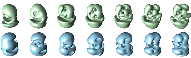
Figure 4. (Bottom) Reconstruction results for EMD-0409 truncated with truncation parameter $L$ varying from $2$ (leftmost) to $8$ (rightmost). (Top) Ground truth structure truncated with truncation parameter $L$ varying from $2$ to $8$.

3.3. Simulation results

We apply Algorithm 2 to two structures from the online EM data bank [62], EMD-0409 [46] and EMD-25892 [65], as well as the Shepp-Logan phantom [85]. For each structure, we run Algorithm 2 for a given value of $L$ and $K$ to obtain a reconstruction. To measure the reconstruction quality, we follow the standard procedure in the cryo-EM community, and compute the Fourier shell correlation (FSC) between the estimated structure and the ground truth. Specifically, the FSC of two structures $\Phi_{1}$ and $\Phi_{2}$ is defined by

(36) $$\text{FSC}(k)=\frac{\sum_{r_{i}:\|r_{i}\|=k}\mathcal{F}\left(\Phi_{1}\right)(r_{i})\overline{\mathcal{F}\left(\Phi_{2}\right)(r_{i})}}{\sqrt{\sum_{\|r_{i}\|=k}|\mathcal{F}\left(\Phi_{1}\right)(r_{i})|^{2}\sum_{\|r_{i}\|=k}|\mathcal{F}\left(\Phi_{2}\right)(r_{i})|^{2}}}.$$

where one structure is the estimated structure, the second is the ground truth, and $\mathcal{F}$ denotes Fourier transform. The FSC is real-valued because of symmetry of the summation. The resolution is determined when the FSC curve drops below $0.5$.

EMD-0409 has dimensions $128\times 128\times 128$, with each voxel having physical length of $1.117$ Å. EMD-25892 has dimensions $320\times 320\times 320$, and voxel size $1.68$ Å. The volumes were downsampled by a factor of 2 and 5, respectively, to give structures of size $64\times 64\times 64$. The ground truth matrices were generated exactly and the matrices $B_{\ell}$ in (31) were generated using $O_{\ell}$ chosen uniformly at random. To fix the units for the Shepp-Logan phantom, we assume the voxels to have side length 1 Å. The simulations used Haar wavelets to define $W$. The simulations set the values of the hyperparameters to $\beta=0.5$ and $K=5000,4000,4000$, for EMD-0409, EMD-25892 and the Shepp-Logan phantom, respectively.

One iteration in Step 4 of Algorithm 2 took around 4.6 seconds on a 2017 MacBook Pro with a 3.1 GHz Intel Core i5 processor and 16 GB of memory. 10000 iterations therefore take around 13 hours.

The result of applying Algorithm 2 to each structure is shown in Figure 3. For all three example structures, during a run of the algorithm, the resolution initially rapidly improves. Afterwards, the improvement slows down and exhibits an exploratory and oscillating behavior. This is typical for RRR-type algorithms, which frequently exhibit a rapid improvement in the early stages of the algorithm, followed by a long exploratory phase, where no improvement is made in the cost function, and then eventually followed by a final phase of rapid improvement. See Figure 5 in [33] for an example in the context of phase retrieval. The results of Algorithm 2 exhibit the rapid initial improvement, but seem to not finish the exploration phase within the considered number of iterations. However, rather than expending more calculation time, Figure 3 shows that Algorithm 2 obtains a reasonable ab initio model within roughly 1000 iterations, which can then be refined using other software packages like RELION or cryoSPARC [86, 81, 76].

One could expect the obtained resolution to partly be limited by the sparsity constraint, since sparsity truncation will remove the finer details, i.e., high frequency information, although the algorithm compensates for this by projecting back onto the correct correlation. A few variations of Algorithm 2 could be considered, inspired by different alternatives to RRR in the phase retrieval literature (e.g., [64]), and one could alternatively allow for values of $K$ that increase with the iteration number in order to gradually increase the resolution.

The FSC curves in Figure 3 differ qualitatively from those obtained by other techniques, with values that typically approximately equal 1 at low resolutions and then fall off sharply at medium frequencies. This behavior is expected whenever the image rotations are accurately estimated. However, we operate at a much lower SNR for which rotations cannot be accurately assigned, leading to the different appearance of the FSC curves.

During the run of the algorithm, the optimal resolutions obtained for the three structures were $17.2$ Å, $20.52$ Å, and $4.59$ Å, respectively, and the resolutions at the initialization of the algorithm were $21.3$ Å, $329.8$ Å, and $8.4$ Å, respectively. As a comparison, the resolutions between the ground truth structures and their truncation into the spherical Bessel bases with the chosen values of $L$ are $6.0$ Å, $18.50$ Å and $2.20$ Å, respectively; these resolutions are bounds on the optimally obtainable resolutions.

Figure 4 also shows a comparison of EMD-0409 with its reconstruction, truncated to different values of $L$. Visually, the reconstructed element captures the relevant features of the ground truth although limited by the resolution expected from Figure 3, for each value of $L$, and the resolution increases with $L$.

Movie 1 visualizes the reconstructed volume as a function of the iteration number. Note that the reconstruction at each step is visually similar to the ground truth, although the computed resolution noticeably improves during the run of the algorithm. This implies that even knowledge of the coefficients $A_{\ell}O_{\ell}$ with the wrong rotation matrices $O_{\ell}$ provides some information about the ground truth.

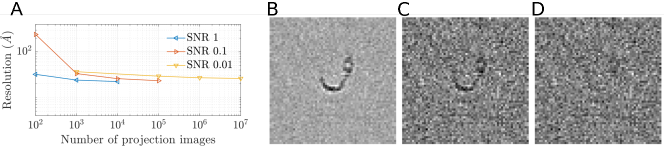
Figure 5. (A) Resolution of reconstructed volume using second moment estimated from noisy projection images. (B–D) Sample CTF-affected and noisy projection images for SNR $1$, $0.1$ and $0.01$, respectively.

We additionally show the result of running Algorithm 2 on EMD-25892 with moments estimated from noisy projection images, which are also affected by contrast transfer functions (CTFs). We generate projection images according to the model

(37) $$I_{R_{i}}(x,y)=h_{i}(x,y)*\int_{z=-\infty}^{\infty}(R_{i}\cdot\Phi)(x,y,z)dz\,+\,\varepsilon(x,y),$$

where $h_{i}$ is a point-spread function. The images were generated using signal-to-noise ratios 1,0.1 and 0.01, with the number of images used ranging between $10^{2}$ and $10^{7}$. All projection images used voltage $300$ kV and spherical aberration $2$ mm. The defocus values ranged between 1 $\mu$m and 4 $\mu$m. When using at most $10^{5}$ projection images, the images used distinct defocus values. For $10^{6}$ and $10^{7}$ images, we divided the images into $10^{4}$ and $10^{3}$ defocus groups, respectively.

We estimate the second moment using the approach in [68]. The result is shown in Fig. 5, with accuracy comparable to that of Fig. 3 when using $\omega(\sigma^{4})$ projection images. The simulations used $\beta=0.5$ and $K=5000$.

4. Discussion

The contribution of this paper is twofold. As the first contribution, our theoretical results imply that a sparse mixture of point masses can be uniquely recovered from the second order moment, even in the case of a uniform distribution of viewing angles, whereas previous work has only proven recovery using the third order moment. Thus, fewer images are required for reconstruction. This has a number of potential experimental implications. Firstly, since microscope time is expensive, this may greatly reduce the cost of the experimental part of the cryo-EM pipeline. This might be especially important for XFEL, where throughput is a major bottleneck and viewing directions are more likely to be uniformly distributed [91, 57]. Secondly, it may enable reconstruction of structures where a limited number of projection images can be captured. This might be the case, for example, when the molecule may appear in several conformational states, and a limited number of images will be available for each conformation.

The second contribution is a new algorithm for ab initio modeling which can be used as a starting point for iterative refinement procedures and additionally provides another way to validate reconstruction results obtained by different computational techniques. The computational framework introduced in this article opens the door to incorporating a number of promising techniques from crystallographic phase retrieval into cryo-EM algorithms. There is, for instance, flexibility in choosing the projection operators $\rho_{1}$ and $\rho_{2}$. It may include biologically-oriented priors, such as minimum atom-atom distance or Wilson statistics [88, 42], or data-driven priors based on previously resolved structures [55]. A systematic study of adapting these techniques will be initiated in coming work. Additional future work includes extending the use of sparsifying priors in other parts of the cryo-EM reconstruction pipeline, for instance in existing approaches to iterative refinement [81] or in autocorrelation analysis using micrographs without particle picking [8, 61, 12]. However, we do not expect sparsity to have as dramatic an impact on the sample complexity in the case of reconstruction directly from micrographs without particle picking. When expanding $L\times L$ projection images in a steerable basis such as the Fourier-Bessel basis [68], the second order moment of picked particles has $\mathcal{O}(L^{3})$ independent entries. This is comparable to the number of parameters required to describe the 3-D structure. Still, in the case of uniform distribution of viewing directions Kam [52] showed that the second order moment is insufficient for 3-D structure recovery, but this paper shows that additional sparsity assumptions ensure unique recovery of a 3-D structure from the second order moment. For autocorrelation analysis of entire micrographs, the second order moment is a 1-D profile equivalent to a rotationally-invariant power spectrum. Therefore, the number of entries is clearly insufficient for 3-D reconstruction and information from the third order moment needs to be incorporated as well. The sparsity constraint may potentially improve the quality of recovery, but the sample complexity is asymptotically the same, proportional to $\sigma^{6}$.

Yet another important direction is to incorporate the sparsity prior into reconstruction by the method of moments when there is a non-uniform distribution of viewing directions [83].

Molecular reconstruction using the method of moments fills an important niche in single-particle reconstruction. Existing software packages like RELION [81], cryoSPARC [76] etc. encounter difficulties when reconstructing small molecules (e.g., below 40 kDa) even though particle picking is not prohibitively difficult at this size [93, Fig. 10f,g,h]. The methods of this paper are therefore viable in situations where other techniques are not expected to be. However, we emphasize that we do not suggest the method of moments to be competitive to RELION or cryoSPARC in terms of resolution for large molecules except for the purpose of validation or fast ab-initio modeling technique. Moreover, we also expect that incorporating sparsity priors would improve the sample complexity and quality of reconstruction algorithms employed by existing software packages like RELION and cryoSPARC. A full demonstration would be an important direction for future work.

Appendix A Proofs of auxiliary results for Theorems 1 and 2

A.1. Proof of Lemma 8

Note that $S_{ij}$ is connected and compact, since $S_{ij}=\theta_{ij}(\operatorname{SO}(3))$ and $\operatorname{SO}(3)$ is compact and connected, while $\theta_{ij}$ is continuous. It also is semialgebraic, as $\operatorname{SO}(3)$ is a real algebraic variety and $\theta_{ij}$ is a polynomial map (see the Tarski-Seidenberg theorem [16]).

Define $T_{ij}\subseteq\mathbb{R}^{2}\times\mathbb{R}^{2}$ as the set cut out by the three constraints in (8). Assume $((x_{1},y_{1}),(x_{2},y_{2}))\in S_{ij}$. By definition of $S_{ij}$, there exist $R\in\operatorname{SO}(3)$ and $z_{1},z_{2}\in\mathbb{R}$ such that $R\mathbf{a}_{i}=(x_{1},y_{1},z_{1})^{\!\top}$ and $R\mathbf{a}_{j}=(x_{2},y_{2},z_{2})^{\!\top}$. Then

$$\|\mathbf{a}_{i}\|^{2}-x_{1}^{2}-y_{1}^{2}=\|R\mathbf{a}_{i}\|^{2}-x_{1}^{2}-y_{1}^{2}=z_{1}^{2},$$

likewise $\|\mathbf{a}_{j}\|^{2}-x_{2}^{2}-y_{2}^{2}=z_{2}^{2},$ and

$$\left(\langle\mathbf{a}_{i},\mathbf{a}_{j}\rangle\!-x_{1}x_{2}\!-y_{1}y_{2}\right)^{2} =\left(\langle R\mathbf{a}_{i},R\mathbf{a}_{j}\rangle\!-x_{1}x_{2}\!-y_{1}y_{2}\right)^{2}$$

$$=(z_{1}z_{2})^{2}.$$

Also, $x_{1}^{2}+y_{1}^{2}\leq\|R\mathbf{a}_{i}\|^{2}=\|\mathbf{a}_{i}\|^{2}$, and similarly $x_{2}^{2}+y_{2}^{2}\leq\|\mathbf{a}_{j}^{2}\|^{2}$. These show that $\left((x_{1},y_{1}),(x_{2},y_{2})\right)\in T_{ij}$, whence $S_{ij}\subseteq T_{ij}$.

For the converse, take $\left((x_{1},y_{1}),(x_{2},y_{2})\right)\in T_{ij}$. Let

$$z_{1}=\sqrt{\|\mathbf{a}_{i}\|^{2}-x_{1}^{2}-y_{1}^{2}}\quad\text{and}\quad z_{2}=\varepsilon\sqrt{\|\mathbf{a}_{j}\|^{2}-x_{2}^{2}-y_{2}^{2}},$$

where $\varepsilon=\operatorname{sign}\left(\langle\mathbf{a}_{i},\mathbf{a}_{j}\rangle-x_{1}x_{2}-y_{1}y_{2}\right)$. Put $\mathbf{b}_{i}=(x_{1},y_{1},z_{1})^{\!\top}$ and $\mathbf{b}_{j}=(x_{2},y_{2},z_{2})^{\!\top}$ in $\mathbb{R}^{3}$. By the choice of $z_{1}$ and $z_{2}$,

(38) $$\|\mathbf{b}_{i}\|=\|\mathbf{a}_{i}\|\quad\text{and}\quad\|\mathbf{b}_{j}\|=\|\mathbf{a}_{j}\|.$$

Also, from the equality constraint in (8), it holds $z_{1}^{2}z_{2}^{2}=\left(\langle\mathbf{a}_{i},\mathbf{a}_{j}\rangle-x_{1}x_{2}-y_{1}y_{2}\right)^{2}$. This with the choice of $\varepsilon$ implies

(39) $$\langle\mathbf{b}_{i},\mathbf{b}_{j}\rangle=\langle\mathbf{a}_{i},\mathbf{a}_{j}\rangle.$$

From (38) and (39), there exists $R\in\operatorname{SO}(3)$ such $\mathbf{b}_{i}=R\mathbf{a}_{i}$ and $\mathbf{b}_{j}=R\mathbf{a}_{j}$. Hence $\left((x_{1},y_{1}),(x_{2},y_{2})\right)\in S_{ij}$, whence $T_{ij}\subseteq S_{ij}$. We conclude $T_{ij}=S_{ij}$.

The dimension of $S_{ij}$ as a semialgebraic set is the maximal dimension of a cell in any cylindrical algebraic decomposition of it [16, Cor. 2.8.9]. This agrees with the maximal rank attained by the differential of $\theta_{ij}$:

$$\dim(S_{ij})=\max_{R}\operatorname{rank}(D\theta_{ij}:T_{R}(\operatorname{SO}(3))\rightarrow T_{\theta_{ij}(R)}(\mathbb{R}^{2}\times\mathbb{R}^{2})),$$

where $T$ denotes tangent space. We recall that the tangent space to rotation matrices is parameterized by skew-symmetric matrices. Specifically, $T_{R}(\operatorname{SO}(3))=\{[s]_{\times}R:s\in\mathbb{R}^{3}\}$, where

$$[s]_{\times}:=\begin{pmatrix}0&s_{3}&-s_{2}\\ -s_{3}&0&s_{1}\\ s_{2}&-s_{1}&0\end{pmatrix}.$$

Then, $D\theta_{ij}([s]_{\times}R)=\left(\pi[s]_{\times}R\mathbf{a}_{i},\pi[s]_{\times}R\mathbf{a}_{j}\right)\in\mathbb{R}^{2}\times\mathbb{R}^{2}=T_{\theta_{ij}(R)}(\mathbb{R}^{2}\times\mathbb{R}^{2})$. Putting $(x_{1},y_{1},z_{1})^{\!\top}:=R\mathbf{a}_{i}$ and $(x_{2},y_{2},z_{2})^{\top}:=R\mathbf{a}_{j}$, we rewrite

$$D\theta_{ij}([s]_{\times}R)=W(R)s,\quad\quad\text{where}~{}W(R):=\begin{pmatrix}0&-z_{1}&y_{1}\\ z_{1}&0&-x_{1}\\ 0&-z_{2}&y_{2}\\ z_{2}&0&-x_{2}\end{pmatrix}.$$

Thus, $\dim(S_{ij})=3$, unless $W(R)$ is rank-deficient for all $R\in\operatorname{SO}(3)$. We claim it is rank-deficient for specific $R$ if and only if $(x_{1},y_{1},z_{1})$ and $(x_{2},y_{2},z_{2})$ are linearly dependent or $z_{1}=z_{2}=0$. This is proven using a computer algebra system, e.g. [44]. Indeed, if $I$ is ideal in the ring $\mathbb{Q}[x_{1},y_{1},z_{1},x_{2},y_{2},z_{2}]$ generated by the $3\times 3$ minors of $W(R)$, the claim follows from calculating the primary decomposition [28]:

$$I=\langle z_{1}y_{2}-y_{1}z_{2},z_{1}x_{2}-x_{1}z_{2},y_{1}x_{2}-x_{1}y_{2}\rangle\cap\langle z_{2}^{2},z_{1}z_{2},z_{1}^{2}\rangle.$$

Given the claim, $\operatorname{rank}(W(R))<3$ for all $R\in\operatorname{SO}(3)$ if and only if $\mathbf{a}_{i}$ and $\mathbf{a}_{j}$ are linearly dependent. In other words, $S_{ij}$ has dimension $3$ if and only if $\mathbf{a}_{i}$ and $\mathbf{a}_{j}$ are linearly independent. The proof of Lemma 8 is complete. ∎

A.2. Proof of Lemma 9

As mentioned in the main text, this is immediate from Definitions 6 and 7 and (10). ∎

A.3. Proof of Lemma 10

If $X$ is a subset of a real Euclidean space $\mathbb{R}^{k}$, we write $\overline{X}$ for the Zariski closure in $\mathbb{R}^{k}$, and $\mathcal{I}(\overline{X})$ for the real radical ideal of $\overline{X}$.

First, note that $\overline{S_{ij}}$ is irreducible. This is because $S_{ij}=\theta_{ij}(\operatorname{SO}(3))$, $\theta_{ij}$ is polynomial and $\operatorname{SO}(3)$ is an irreducible algebraic variety. So, $\mathcal{I}(\overline{S_{ij}})$ is prime [16, Thm. 2.8.3(ii)]. Also, $\overline{S}_{ij}$ has dimension $3$ as an algebraic variety. This is by [16, Prop. 2.8.2], and Lemma 8 which states $S_{ij}$ has dimension $3$ as a semialgebraic set. So, $\mathcal{I}(\overline{S_{ij}})$ has height $1$ [16, Def. 2.8.1]. Here, every prime ideal with height $1$ is principal, as $\mathbb{R}[x_{1},y_{1},x_{2},y_{2}]$ is a unique factorization domain. It follows that

(40) $$\mathcal{I}(\overline{S_{ij}})=\langle f\rangle,$$

for some irreducible polynomial $f\in\mathbb{R}[x_{1},y_{1},x_{2},y_{2}]$, where angle brackets indicate ideal generation.

By Lemma 8, we know $S_{ij}\subseteq\mathcal{Z}(q_{ij})$, where $\mathcal{Z}$ denotes the zero set in $\mathbb{R}^{2}\times\mathbb{R}^{2}$. Taking closures, $\overline{S_{ij}}\subseteq\mathcal{Z}(q_{ij})$. Equivalently, $q_{ij}\in\mathcal{I}(\overline{S_{ij}})$. By (40), this means $f$ evenly divides $q_{ij}$, say,

(41) $$q_{ij}=fg,$$

for some $g\in\mathbb{R}[x_{1},y_{1},x_{2},y_{2}]$. To conclude the proof, it suffices to prove that $g$ is a nonzero scalar. Then $\langle q_{ij}\rangle=\langle f\rangle=\mathcal{I}(\overline{S_{ij}})$, and $q_{ij}$ is irreducible because $f$ is.

For a contradiction, assume that $f$ has positive degree. Then, (41) implies

(42) $$(q_{ij})_{\text{top}}=f_{\text{top}}g_{\text{top}},$$

where the subscript indicates the top total degree part of the polynomial. Here,

$$q_{ij}= \left(\|\mathbf{a}_{i}\|^{2}\|\mathbf{a}_{j}\|^{2}-\langle\mathbf{a}_{i},\mathbf{a}_{j}\rangle^{2}\right)-\|\mathbf{a}_{j}\|^{2}x_{1}^{2}-\|\mathbf{a}_{j}\|^{2}y_{1}^{2}-\|\mathbf{a}_{i}\|^{2}x_{2}^{2}-\|\mathbf{a}_{i}\|^{2}y_{2}^{2}$$

(43) $$+2\langle\mathbf{a}_{i},\mathbf{a}_{j}\rangle x_{1}x_{2}+2\langle\mathbf{a}_{i},\mathbf{a}_{j}\rangle y_{1}y_{2}+x_{1}^{2}y_{2}^{2}+y_{1}^{2}x_{2}^{2}-2x_{1}y_{1}x_{2}y_{2}.$$

Thus,

$$(q_{ij})_{\text{top}}=x_{1}^{2}y_{2}^{2}+y_{1}^{2}x_{2}^{2}-2x_{1}y_{1}x_{2}y_{2}=(x_{1}y_{2}-y_{1}x_{2})^{2}.$$

From (42), the assumption that $f$ has positive degree and unique factorization, we deduce that (possibly after multiplying by nonzero scalars)

$$f_{\text{top}}=g_{\text{top}}=x_{1}y_{2}-y_{1}x_{2}.$$

Therefore,

$$f=x_{1}y_{2}-x_{2}y_{1}+\alpha x_{1}+\beta y_{1}+\gamma x_{2}+\delta y_{2}+\varepsilon,$$

(44) $$g=x_{1}y_{2}-x_{2}y_{1}+\zeta x_{1}+\eta y_{1}+\theta x_{2}+\iota y_{2}+\kappa,$$

for some $\alpha,\beta,\gamma,\delta,\varepsilon,\zeta,\eta,\theta,\iota,\kappa\in\mathbb{R}$. Now we insert (A.3) and (A.3) into (41). Equating the constants and the coefficients of $x_{1}^{2},y_{1}^{2},x_{2}^{2},y_{2}^{2}$ gives

(45) $$\begin{cases}\|\mathbf{a}_{i}\|^{2}\|\mathbf{a}_{j}\|^{2}-\langle\mathbf{a}_{i},\mathbf{a}_{j}\rangle^{2}=\varepsilon\kappa\\ -\|\mathbf{a}_{j}\|^{2}=\alpha\zeta\\ -\|\mathbf{a}_{j}\|^{2}=\beta\eta\\ -\|\mathbf{a}_{i}\|^{2}=\gamma\theta\\ -\|\mathbf{a}_{i}\|^{2}=\delta\iota.\end{cases}$$

All the left-hand sides in (45) are nonzero because $\mathbf{a}_{i}$ and $\mathbf{a}_{j}$ are linearly independent. Therefore, $\alpha,\ldots,\kappa$ are all nonzero. Next, we equate the coefficients of $x_{1},y_{1},x_{2},y_{2}$ in (41). The result is that

$$\begin{pmatrix}\alpha&\zeta\\ \beta&\eta\\ \gamma&\theta\\ \delta&\iota\end{pmatrix}\!\!\begin{pmatrix}\kappa\\ \varepsilon\end{pmatrix}=0,$$

whence the $4\times 2$ matrix has rank $1$. So all its $2\times 2$ minors vanish, in particular

(46) $$\alpha\eta-\beta\zeta=0.$$

Finally, we equate the coefficients of $x_{1}y_{1}$ in (41):

(47) $$0=\alpha\eta+\beta\zeta.$$

(46) and (47) imply

(48) $$\alpha\eta=\beta\zeta=0.$$

But this contradicts the earlier finding that $\alpha,\ldots,\kappa$ are all nonzero. So the assumption that $f$ has positive degree is false, and $f$ is a nonzero scalar. This proves Lemma 10. ∎

A.4. Proof of Corollary 11

By Lemma 9, the support of $M_{2}$ is $\cup_{i,j=1}^{p}S_{ij}$. This has Zariski closure $\cup_{i,j=1}^{p}\overline{S_{ij}}$. We claim its irredundant irreducible decomposition is

(49) $$\{(\mathbf{x}_{1},\mathbf{x}_{2}):\mathbf{x}_{1}=\mathbf{x}_{2}\}\,\,\cup\,\,\bigcup_{i\neq j}\overline{S_{ij}}.$$

The claim follows from several facts. First, for all $i\neq j$, $\overline{S_{ij}}$ is irreducible. It has dimension $3$ and defining equation $q_{ij}$ (A.3), by A1 and Lemma 10. When $i\neq j$, $i^{\prime}\neq j^{\prime}$ and $(i,j)\neq(i^{\prime},j^{\prime})$, then $q_{ij}$ and $q_{i^{\prime}j^{\prime}}$ are not scalar multiples of each other by A2 (cf. their coefficients on $x_{1}^{2},x_{2}^{2},x_{1}^{2}y_{1}^{2}$). Hence $\overline{S_{ij}}\neq\overline{S_{i^{\prime}j^{\prime}}}$. Next, $\overline{S_{ii}}=\{(\mathbf{x}_{1},\mathbf{x}_{2}):\mathbf{x}_{1}=\mathbf{x}_{2}\}$ (all $i$). Further, $\{(\mathbf{x}_{1},\mathbf{x}_{2}):\mathbf{x}_{1}=\mathbf{x}_{2}\}\nsubseteq\overline{S_{ij}}$ (all $i\neq j$), because when we substitute $x_{1}=x_{2}$ and $y_{1}=y_{2}$ into (A.3) we get a nonzero result as the constant term does not vanish. All together, (49) is the claimed irredundant irreducible decomposition as wanted. ∎

A.5. Proof of Lemma 13

This follows from $\mathcal{I}(\overline{S_{ij}})=\langle q_{ij}\rangle$ (Lemma 10), the expression (A.3) for $q_{ij}$, and the proof of [20, Thm. 3]. ∎

A.6. Proof of Lemma 14

From (15), we have

$$M_{2}(S_{ij})=\sum_{i^{\prime},j^{\prime}=1}^{p}w_{i^{\prime}}w_{j^{\prime}}\mu(\theta_{i^{\prime}j^{\prime}}^{-1}(S_{ij})).$$

Here $\mu(\theta_{ij}^{-1}(S_{ij}))=\mu(\operatorname{SO}(3))=1$ by definition of $S_{ij}$. On the other hand, for all $i^{\prime},j^{\prime}=1,\ldots,p$ with $(i^{\prime},j^{\prime})\neq(i,j)$, $S_{ij}\cap S_{i^{\prime}j^{\prime}}$ is a semialgebraic set with positive codimension in $S_{i^{\prime}j^{\prime}}$ by the fact that (49) is an irredundant irreducible decomposition. Then $\theta_{i^{\prime}j^{\prime}}^{-1}(S_{ij})=\theta_{i^{\prime}j^{\prime}}^{-1}(S_{ij}\cap S_{i^{\prime}j^{\prime}})$ is a semialgebraic set with positive codimension in $\operatorname{SO}(3)$. Since $\mu$ is absolutely continuous, it implies $\mu(\theta_{i^{\prime}j^{\prime}}^{-1}(S_{ij}))=0$. (25) follows. ∎

Appendix B Proof of Theorem 3

We show how to reduce the proof to an application of Theorem 1. We have

(50) $$R\cdot\Phi(\mathbf{x})=\sum_{i=1}^{p}w_{i}e^{-\frac{\|R\mathbf{x}-\mathbf{a}_{i}\|^{2}}{2\kappa^{2}}}=\sum_{i=1}^{p}w_{i}e^{-\frac{\|\mathbf{x}-R^{T}\mathbf{a}_{i}\|^{2}}{2\kappa^{2}}}.$$

Writing $\mathbf{x}=(x,y,z)$ gives the following expression for the projection images

(51) $$\begin{split}I_{R}(x,y)&=\sum_{i=1}^{p}w_{i}e^{-\frac{\|(x,y)-\pi R^{T}\mathbf{a}_{i}\|^{2}}{2\kappa^{2}}}\int_{-\infty}^{\infty}e^{-\frac{(z-\pi_{z}R^{T}\mathbf{a}_{i})}{2\kappa^{2}}}dz\\ &=\sum_{i=1}^{p}\sqrt{2\pi}\kappa w_{i}e^{-\frac{\|(x,y)-\pi R^{T}\mathbf{a}_{i}\|^{2}}{2\kappa^{2}}},\end{split}$$

where $\pi_{z}(a_{1},a_{2},a_{3}):=a_{3}$ is the projection operator onto the last coordinate. The second moment $M_{2}^{G}$ can then be written as

(52) $$\begin{split}&M_{2}^{G}((x_{1},y_{1}),(x_{2},y_{2}))\\ &=\!\!\sum_{i,j=1}^{p}2\pi\kappa^{2}w_{i}w_{j}\int_{\operatorname{SO}(3)}\!\!\!\!\!\!\!\!\!\!e^{-\frac{\|(x_{1},y_{1})-\pi R^{T}\mathbf{a}_{i}\|^{2}+\|(x_{2},y_{2})-\pi R^{T}\mathbf{a}_{j}\|^{2}}{2\kappa^{2}}}d\mu(R)\\ &=\!\!\sum_{i,j=1}^{p}2\pi\kappa^{2}w_{i}w_{j}\int_{\operatorname{SO}(3)}\!\!\!\!\!\!\!\!\!\!e^{-\frac{\|(x_{1},y_{1})-\pi R\mathbf{a}_{i}\|^{2}+\|(x_{2},y_{2})-\pi R\mathbf{a}_{j}\|^{2}}{2\kappa^{2}}}d\mu(R)\\ &=2\pi\kappa^{2}M_{2}*(k\otimes k),\end{split}$$

where the second equality used the fact that the Haar measure on $\operatorname{SO}(3)$ is invariant to transpositions [56, Theorem 4.36], and $M_{2}$ is the second moment in the model of Theorem 1. Since $k$ has non-vanishing Fourier-transform, this equation can be deconvolved to obtain $M_{2}$. By Theorem 1, $M_{2}$ determines the weights and atomic positions $(w_{i},\mathbf{a}_{i})$ up to a joint rotation and reflection, which concludes the proof.

∎

Appendix C Sample complexity: Proofs of Theorems 4 and Corollary 5

C.1. Proof of Theorem 4

The proof is divided into several steps.

Step 0: We state a general fact about real analytic functions that we will use: Let $H(\mathbf{y},\mathbf{z}):\mathbb{R}^{m}\times\mathbb{R}^{n}\rightarrow\mathbb{R}$ be real analytic jointly in $(\mathbf{y},\mathbf{z})$. Let $\nu$ be a compactly supported and absolutely continuous measure on $\mathbb{R}^{n}$. Then $\int H(\mathbf{y},\mathbf{z})d\nu(\mathbf{z})$ is real-analytic in $\mathbf{y}$. This can be justified by appropriately differentiating under the integral sign, see [37].

Step 1: We introduce notation.

First, define

(53) $$X=(B(0,r)\times[w_{-},w_{+}])^{\times p}\subseteq\mathbb{R}^{4p},$$

where $B(0,r)$ is the $\ell^{2}$-ball of radius $r$ in $\mathbb{R}^{3}$ centered at $0$. $X$ is the space of possible molecules.

Next, slightly modifying the notation in the main text, write

$${M}_{2}^{[m]}:X\rightarrow\mathbb{R}^{2^{m}\times 2^{m}}\!\otimes\mathbb{R}^{2^{m}\times 2^{m}}$$

for the map associating a molecule to its pixelated second moment ((13)) when $2^{m}\times 2^{m}$ pixels are used. Explicitly,

$${M}_{2}^{[m]}(\left\{(\mathbf{a}_{i},w_{i})\right\})=$$

$$\Bigg{\{}\int_{j_{4}\tau}^{(j_{4}+1)\tau}\!\int_{j_{3}\tau}^{(j_{3}+1)\tau}\!\int_{j_{2}\tau}^{(j_{2}+1)\tau}\!\int_{j_{1}\tau}^{(j_{1}+1)\tau}\!\int_{\operatorname{SO}(3)}\sum_{i,j=1}^{p}w_{i}w_{j}\delta_{\pi R\mathbf{a}_{i}}(x_{1},y_{1})\delta_{\pi R\mathbf{a}_{j}}(x_{2},y_{2})$$

$$\qquad\qquad\qquad\qquad\qquad\qquad\qquad\qquad\ast(k(x_{1},y_{1})k(x_{2},y_{2}))d\mu(R)dx_{1}dy_{1}dx_{2}dy_{2}\Bigg{\}},$$

for $j_{1},j_{2},j_{3},j_{4}\in\{-2^{m-1},\ldots,2^{m-1}-1\}$. Then, ${M}^{[m]}_{2}$ is a real analytic function by Step 0. Indeed, the Gaussian kernel $k(x,y)$ is real analytic, so the above integrand is real analytic in all variables. (Also, integration over $\operatorname{SO}(3)$ is replaced by integration against a compactly supported absolutely continuous measure on $\mathbb{R}^{3}$ if we parameterize $\operatorname{SO}(3)$ with Euler angles.)

Thirdly, we put

$$L^{[m]}:\mathbb{R}^{2^{m+1}\!\times 2^{m+1}}\!\otimes\mathbb{R}^{2^{m+1}\!\times 2^{m+1}}\rightarrow\mathbb{R}^{2^{m}\!\times 2^{m}}\!\otimes\mathbb{R}^{2^{m}\!\times 2^{m}}$$

for the obvious linear map which lowers the resolution of the second moment by a factor of two, i.e. $L^{[m]}(t)=s$ where

$$s_{j_{1},j_{2},j_{3},j_{4}}=\sum_{\gamma_{4}\in\{0,1\}}\sum_{\gamma_{3}\in\{0,1\}}\sum_{\gamma_{2}\in\{0,1\}}\sum_{\gamma_{1}\in\{0,1\}}t_{2j_{1}+\gamma_{1},2j_{2}+\gamma_{2},2j_{3}+\gamma_{3},2j_{4}+\gamma_{4}}$$

for $j_{1},j_{2},j_{3},j_{4}\in\{-2^{m-1},\ldots,2^{m-1}-1\}$. For all $m$, it holds

(54) $${M}^{[m]}_{2}=L^{[m]}\circ{M}_{2}^{[m+1]}.$$

Step 2: We prove that a certain stabilization occurs as $m\rightarrow\infty$.

Consider $X^{\times 2}=(B(0,r)\times[w_{-},w_{+}])^{\times p}\times(B(0,r)\times[w_{-},w_{+}])^{\times p}\subseteq\mathbb{R}^{8p}$, where the variables on $\mathbb{R}^{8p}$ are $\{(\mathbf{a}_{i},w_{i})\},\{(\mathbf{b}_{i},v_{i})\}$. Regard $X^{\times 2}$ as a semianalytic set (i.e., a subset of Euclidean space locally defined by real analytic equations and inequalities). Let $\mathcal{O}(X^{\times 2})$ denote the ring of real analytic functions on $X$. Then $\mathcal{O}(X^{\times 2})$ is a Noetherian ring, because $X$ is compact [39, Théorème I, 9]. (Note that $X^{\times 2}$ automatically satisfies the Stein hypothesis in loc. cit. since we are in the real case, see [90].).

We define

$$\begin{split}\mathcal{I}^{[m]}=\text{ ideal in }&\mathcal{O}(X^{\times 2})\text{ generated by the }2^{4m}\text{ coordinate functions of }\\ &M_{2}^{[m]}(\{(\mathbf{a}_{i},w_{i})\})-{M_{2}^{[m]}}(\{(\mathbf{b}_{i},v_{i})\}).\end{split}$$

For all $m$, we have

$$\mathcal{I}^{[m+1]}\supseteq\mathcal{I}^{[m]}$$

by (54). From Noetherianity, there exists $m^{\prime}=m^{\prime}(p,r,w_{+},w_{-})$ such that

$$\mathcal{I}^{[m]}=\mathcal{I}^{[m^{\prime}]}\quad\,\,\,\forall m\geq m^{\prime}.$$

Thus the corresponding zero sets in $X^{\times 2}$ stabilize too:

$$\Big{\{}\big{(}\{(\mathbf{a}_{i},w_{i})\},\{(\mathbf{b}_{i},v_{i})\}\big{)}:\,{M}_{2}^{[m]}(\{(\mathbf{a}_{i},w_{i})\})={M}_{2}^{[m]}(\{(\mathbf{b}_{i},v_{i})\})\Big{\}}\subseteq X^{\times 2}$$

is constant in $m$ if $m\geq m^{\prime}$. Equivalently, for all $\{(\mathbf{a}_{i},w_{i})\}\in X$ we have:

(55) $$\text{the fiber }\,({M}_{2}^{[m]})^{-1}\!\big{(}{M}_{2}^{[m]}(\{\mathbf{a}_{i},w_{i}\})\big{)}\!\subseteq X\,\,\text{ is constant in }m\text{ if }m\geq m^{\prime}.$$

Step 3: We deduce an equality in which there is no pixelation.

Specifically, fix $\{(\mathbf{a}_{i},w_{i})\},\{(\mathbf{b}_{i},v_{i})\}\in X$ such that $\{(\mathbf{a}_{i},w_{i})\}$ satisfies A1-A2 in the main text and

(56) $${M}_{2}^{[m^{\prime}]}(\{(\mathbf{a}_{i},w_{i})\})={M}_{2}^{[m^{\prime}]}(\{(\mathbf{b}_{i},v_{i})\})$$

holds. We claim there is an equality between unpixelated (but still blurred) second moments:

(57) $$M_{2}(\{(\mathbf{a}_{i},w_{i})\})\ast(k\otimes k)=\,M_{2}(\{(\mathbf{b}_{i},v_{i})\})\ast(k\otimes k).$$

To see this, note by Step 0 that both sides of (57) are real-valued real analytic functions on $\mathbb{R}^{2}\times\mathbb{R}^{2}$. From continuity, if they differ on $[-1,1]^{2}$ there must exist a product of sufficiently small pixels where their integrals differ, i.e. $m\geq m^{\prime}$ and $j_{1},j_{2},j_{3},j_{4}\in\{-2^{m-1},\ldots,2^{m-1}-1\}$ such that

(58) $$M_{2}^{[m]}(\{(\mathbf{a}_{i},w_{i})\})((j_{1},j_{2}),(j_{3},j_{4}))\,\neq\,M_{2}^{[m]}(\{(\mathbf{b}_{i},v_{i})\})((j_{1},j_{2}),(j_{3},j_{4})).$$

However, (58) contradicts (56) and (55). Thus, (57) holds on $[-1,1]^{2}\times[-1,1]^{2}$. By real analyticity, (57) then holds on all of $\mathbb{R}^{2}\times\mathbb{R}^{2}$ as wanted.

Step 4: We undo the Gaussian blurring.

Continue with (57). Because $M_{2}(\cdot)$ is compactly supported, it identifies with a tempered distribution. The Fourier transform is thus applicable to (57). By the convolution theorem [47, Thm. 7.1.15], it gives

(59) $$\widehat{M_{2}}(\{(\mathbf{a}_{i},w_{i})\})\,\widehat{k\otimes k}\,\,\,=\,\,\widehat{M_{2}}(\{(\mathbf{b}_{i},v_{i})\}\,\widehat{k\otimes k}.$$

Note that the Paley-Wiener theorem [47, Thm. 7.1.14] implies $\widehat{M_{2}}(\cdot)$ is a function rather just a distribution (moreover it is extendable to an entire function). Also, $\widehat{k\otimes k}$ is a Gaussian function. Therefore, (59) can be regarded as an equality of functions rather than just distributions. Since $\widehat{k\otimes k}\neq 0$ everywhere, it implies

$$\widehat{M_{2}}(\{(\mathbf{a}_{i},w_{i})\})\,\,=\,\,\widehat{M_{2}}(\{(\mathbf{b}_{i},v_{i})\}),$$

whence

(60) $$M_{2}(\{(\mathbf{a}_{i},w_{i})\})=M_{2}(\{(\mathbf{b}_{i},v_{i})\}),$$

using the fact that the Fourier transform is an automorphism on tempered distributions.

Step 5: We use Theorem 2 to conclude.

The above steps have shown: there exists $m^{\prime}=m^{\prime}(p,r,w_{+},w_{-})$ such that if $m\geq m^{\prime}$ then $\{(\mathbf{a}_{i},w_{i})\},\{(\mathbf{b}_{i},v_{i})\}\in X$ and $M_{2}^{[m]}(\{(\mathbf{a}_{i},w_{i})\})=M_{2}^{[m^{\prime}]}(\{(\mathbf{b}_{i},v_{i})\})$ imply $M_{2}(\{(\mathbf{a}_{i},w_{i})\})=M_{2}(\{(\mathbf{b}_{i},v_{i})\})$. However by Theorem 2, $M_{2}(\{(\mathbf{a}_{i},w_{i})\})=M_{2}(\{(\mathbf{b}_{i},v_{i})\})$ implies $\{(\mathbf{a}_{i},w_{i})\}$ and $\{(\mathbf{b}_{i},v_{i})\}$ are equal up to a rotation/reflection in $\mathbb{R}^{3}$, provided $\{(\mathbf{a}_{i},w_{i})\}$ satisfies A1-A2.

The proof of Theorem 4 is complete. ∎

C.2. Proof of Corollary 5

This now follows immediately from [4, Sec. 3] or [73, Sec. 2], because by Theorem 4 the second moment ${M_{2}}^{[m]}(\{(\mathbf{a}_{i},w_{i})\})$ uniquely determines the signal $\{(\mathbf{a}_{i},w_{i})\}$ up to the group action of $O(3)$, provided $\{(\mathbf{a}_{i},w_{i})\}$ satisfies the Zariski-open conditions A1-A2. ∎

Appendix D Normalized Bessel functions and the Nyquist criterion

The spherical Bessel basis defined in the main text uses the normalized spherical Bessel functions $j_{\ell s}(k)$ defined by

(61) $$j_{\ell s}(k)=\frac{1}{c\sqrt{\pi}|j_{\ell+1}(R_{\ell,s})|}j_{\ell}(R_{\ell,s}\frac{k}{c}),$$

where $j_{\ell}$ is the $\ell$th spherical Bessel function of the first kind [25, Eq. 10.2.1], $c$ the bandlimit of the projection images and $R_{\ell,s}$ the $s$th positive solution to $j_{\ell}=0$. The Nyquist criterion determines the maximally allowable value of the truncation parameter $S_{\ell}$ by defining $S_{\ell}$ as the largest integer $s$ satisfying,

(62) $$R_{\ell,s+1}\leq 2\pi cR,$$

assuming the projection images are supported on a disk of radius $R$ [15]. Our numerical experiments used $c=0.5$ and a radius $R$ of $32$ voxels.

References

- [1] Emmanuel Abbe, Joao M Pereira, and Amit Singer. Estimation in the group action channel. In 2018 IEEE International Symposium on Information Theory (ISIT), pages 561–565. IEEE, 2018.
- [2] Larry C Andrews. Special Functions of Mathematics for Engineers, volume 49. Spie Press, 1998.
- [3] Xiao-Chen Bai, Greg McMullan, and Sjors HW Scheres. How cryo-EM is revolutionizing structural biology. Trends in Biochemical Sciences, 40(1):49–57, 2015.
- [4] Afonso S Bandeira, Ben Blum-Smith, Joe Kileel, Amelia Perry, Jonathan Weed, and Alexander S Wein. Estimation under group actions: recovering orbits from invariants. arXiv preprint arXiv:1712.10163, 2017.
- [5] Alexander H Barnett, Charles L Epstein, Leslie Greengard, and Jeremy Magland. Geometry of the Phase Retrieval Problem: Graveyard of Algorithms. Cambridge University Press, 2022.
- [6] Tamir Bendory, Alberto Bartesaghi, and Amit Singer. Single-particle cryo-electron microscopy: Mathematical theory, computational challenges, and opportunities. IEEE Signal Processing Magazine, 37(2):58–76, 2020.
- [7] Tamir Bendory, Robert Beinert, and Yonina C Eldar. Fourier phase retrieval: Uniqueness and algorithms. In Compressed Sensing and its Applications, pages 55–91. Springer, 2017.
- [8] Tamir Bendory, Nicolas Boumal, William Leeb, Eitan Levin, and Amit Singer. Toward single particle reconstruction without particle picking: Breaking the detection limit. arXiv preprint arXiv:1810.00226, 2018.
- [9] Tamir Bendory and Dan Edidin. Toward a mathematical theory of the crystallographic phase retrieval problem. SIAM Journal on Mathematics of Data Science, 2(3):809–839, 2020.
- [10] Tamir Bendory and Dan Edidin. Algebraic theory of phase retrieval. arXiv preprint arXiv:2203.02774, 2022.
- [11] Tamir Bendory and Dan Edidin. The sample complexity of sparse multi-reference alignment and single-particle cryo-electron microscopy. arXiv preprint arXiv:2210.15727, 2022.
- [12] Tamir Bendory, Ti-Yen Lan, Nicholas F. Marshall, Iris Rukshin, and Amit Singer. Multi-target detection with rotations. Inverse Problems and Imaging, 17(2):362–380, 2023.
- [13] Tamir Bendory, Oscar Mickelin, and Amit Singer. Sparse multi-reference alignment: Sample complexity and computational hardness. In ICASSP 2022-2022 IEEE International Conference on Acoustics, Speech and Signal Processing (ICASSP), pages 8977–8981. IEEE, 2022.
- [14] Tejal Bhamre, Teng Zhang, and Amit Singer. Orthogonal matrix retrieval in cryo-electron microscopy. In 2015 IEEE 12th International Symposium on Biomedical Imaging (ISBI), pages 1048–1052. IEEE, 2015.
- [15] Tejal Bhamre, Teng Zhang, and Amit Singer. Anisotropic twicing for single particle reconstruction using autocorrelation analysis. arXiv preprint arXiv:1704.07969, 2017.
- [16] Jacek Bochnak, Michel Coste, and Marie-Françoise Roy. Real Algebraic Geometry, volume 36. Springer Science & Business Media, 2013.
- [17] T Tony Cai, Xiaodong Li, and Zongming Ma. Optimal rates of convergence for noisy sparse phase retrieval via thresholded Wirtinger flow. The Annals of Statistics, 44(5):2221–2251, 2016.
- [18] Ewen Callaway. Revolutionary cryo-EM is taking over structural biology. Nature, 578(7794):201–202, 2020.
- [19] Emmanuel J Candès, Justin Romberg, and Terence Tao. Robust uncertainty principles: Exact signal reconstruction from highly incomplete frequency information. IEEE Transactions on Information Theory, 52(2):489–509, 2006.
- [20] Justin Chen and Joe Kileel. Numerical implicitization. Journal of Software for Algebra and Geometry, 9(1):55–63, 2019.
- [21] Muyuan Chen and Steven J Ludtke. Deep learning-based mixed-dimensional Gaussian mixture model for characterizing variability in cryo-EM. Nature Methods, 18(8):930–936, 2021.
- [22] Ward Cheney and Allen A Goldstein. Proximity maps for convex sets. Proceedings of the American Mathematical Society, 10(3):448–450, 1959.
- [23] Yuejie Chi. Guaranteed blind sparse spikes deconvolution via lifting and convex optimization. IEEE Journal of Selected Topics in Signal Processing, 10(4):782–794, 2016.
- [24] Ingrid Daubechies. Ten lectures on wavelets. SIAM, 1992.
- [25] NIST Digital Library of Mathematical Functions, http://dlmf.nist.gov/, Release 1.1.5 of 2022-03-15. F. W. J. Olver, A. B. Olde Daalhuis, D. W. Lozier, B. I. Schneider, R. F. Boisvert, C. W. Clark, B. R. Miller, B. V. Saunders, H. S. Cohl, and M. A. McClain, eds.
- [26] Jeffrey J Donatelli, Peter H Zwart, and James A Sethian. Iterative phasing for fluctuation X-ray scattering. Proceedings of the National Academy of Sciences, 112(33):10286–10291, 2015.
- [27] David L Donoho. Compressed sensing. IEEE Transactions on Information Theory, 52(4):1289–1306, 2006.
- [28] David Eisenbud. Commutative Algebra: With a View Toward Algebraic Geometry, volume 150. Springer Science & Business Media, 2013.
- [29] Michael Elad. Sparse and Redundant Representations: From Theory to Applications in Signal and Image Processing, volume 2. Springer, 2010.
- [30] Yonina C Eldar and Gitta Kutyniok. Compressed sensing: theory and applications. Cambridge university press, 2012.
- [31] Veit Elser. Phase retrieval by iterated projections. Journal of the Optical Society of America A, 20(1):40–55, 2003.
- [32] Veit Elser. The complexity of bit retrieval. IEEE Transactions on Information Theory, 64(1):412–428, 2017.
- [33] Veit Elser, Ti-Yen Lan, and Tamir Bendory. Benchmark problems for phase retrieval. SIAM Journal on Imaging Sciences, 11(4):2429–2455, 2018.
- [34] Veit Elser, I Rankenburg, and P Thibault. Searching with iterated maps. Proceedings of the National Academy of Sciences, 104(2):418–423, 2007.
- [35] Zhou Fan, Roy R Lederman, Yi Sun, Tianhao Wang, and Sheng Xu. Maximum likelihood for high-noise group orbit estimation and single-particle cryo-EM. arXiv preprint arXiv:2107.01305, 2021.
- [36] James R Fienup. Phase retrieval algorithms: A comparison. Applied Optics, 21(15):2758–2769, 1982.
- [37] Daniel Fischer. Convolution of measurable function with analytic function. Mathematics Stack Exchange, 2013. URL:https://math.stackexchange.com/q/591021 (version: 2013-12-03).
- [38] Joachim Frank. Three-Dimensional Electron Microscopy of Macromolecular Assemblies: Visualization of Biological Molecules in Their Native State. Oxford University Press, 2006.
- [39] Jacques Frisch. Points de platitude d’un morphisme d’espaces analytiques complexes. Inventiones Mathematicae, 4(2):118–138, 1967.
- [40] Simona Galli. X-ray crystallography: One century of Nobel Prizes. Journal of Chemical Education, 91(12):2009–2012, 2014.
- [41] Subhroshekhar Ghosh and Philippe Rigollet. Sparse multi-reference alignment: Phase retrieval, uniform uncertainty principles and the beltway problem. Foundations of Computational Mathematics, pages 1–48, 2022.
- [42] Marc Aurèle Gilles and Amit Singer. A molecular prior distribution for Bayesian inference based on Wilson statistics. Computer Methods and Programs in Biomedicine, 221:106830, 2022.
- [43] Ian Goodfellow, Yoshua Bengio, and Aaron Courville. Deep learning. MIT press, 2016.
- [44] Daniel R. Grayson and Michael E. Stillman. Macaulay2, a software system for research in algebraic geometry, Available at http://www.math.uiuc.edu/Macaulay2/.
- [45] Ido Greenberg and Yoel Shkolnisky. Common lines modeling for reference free ab-initio reconstruction in cryo-EM. Journal of Structural Biology, 200(2):106–117, 2017.
- [46] Mark A Herzik, Mengyu Wu, and Gabriel C Lander. High-resolution structure determination of sub-100 kDa complexes using conventional cryo-EM. Nature Communications, 10(1):1–9, 2019.
- [47] Lars Hörmander. The Analysis of Linear Partial Differential Operators I: Distribution Theory and Fourier Analysis. Springer, 2015.
- [48] Shuai Huang, Mona Zehni, Ivan Dokmanić, and Zhizhen Zhao. Orthogonal matrix retrieval with spatial consensus for 3d unknown-view tomography. arXiv preprint arXiv:2207.02985, 2022.
- [49] Kishore Jaganathan, Samet Oymak, and Babak Hassibi. Sparse phase retrieval: Uniqueness guarantees and recovery algorithms. IEEE Transactions on Signal Processing, 65(9):2402–2410, 2017.
- [50] Slavica Jonić and Carlos Óscar Sánchez Sorzano. Coarse-graining of volumes for modeling of structure and dynamics in electron microscopy: Algorithm to automatically control accuracy of approximation. IEEE Journal of Selected Topics in Signal Processing, 10(1):161–173, 2015.
- [51] Paul Joubert and Michael Habeck. Bayesian inference of initial models in cryo-electron microscopy using pseudo-atoms. Biophysical Journal, 108(5):1165–1175, 2015.
- [52] Zvi Kam. The reconstruction of structure from electron micrographs of randomly oriented particles. Journal of Theoretical Biology, 82(1):15–39, 1980.
- [53] Anya Katsevich and Afonso S Bandeira. Likelihood maximization and moment matching in low SNR Gaussian mixture models. Communications on Pure and Applied Mathematics, 2020.
- [54] Takeshi Kawabata. Gaussian-input Gaussian mixture model for representing density maps and atomic models. Journal of Structural Biology, 203(1):1–16, 2018.
- [55] Dari Kimanius, Gustav Zickert, Takanori Nakane, Jonas Adler, Sebastian Lunz, C-B Schönlieb, Ozan Öktem, and Sjors HW Scheres. Exploiting prior knowledge about biological macromolecules in cryo-EM structure determination. IUCrJ, 8(1):60–75, 2021.
- [56] Alexander A Kirillov. An introduction to Lie groups and Lie algebras, volume 113. Cambridge University Press, 2008.
- [57] Henry J Kirkwood, Raphael de Wijn, Grant Mills, Romain Letrun, Marco Kloos, Mohammad Vakili, Mikhail Karnevskiy, Karim Ahmed, Richard J Bean, Johan Bielecki, et al. A multi-million image Serial Femtosecond Crystallography dataset collected at the European XFEL. Scientific Data, 9(1):1–7, 2022.
- [58] Werner Kühlbrandt. The resolution revolution. Science, 343(6178):1443–1444, 2014.
- [59] RP Kurta, R Dronyak, Massimo Altarelli, Edgar Weckert, and IA Vartanyants. Solution of the phase problem for coherent scattering from a disordered system of identical particles. New journal of physics, 15(1):013059, 2013.
- [60] Ruslan P Kurta, Jeffrey J Donatelli, Chun Hong Yoon, Peter Berntsen, Johan Bielecki, Benedikt J Daurer, Hasan DeMirci, Petra Fromme, Max Felix Hantke, Filipe RNC Maia, et al. Correlations in scattered X-ray laser pulses reveal nanoscale structural features of viruses. Physical review letters, 119(15):158102, 2017.
- [61] Ti-Yen Lan, Tamir Bendory, Nicolas Boumal, and Amit Singer. Multi-target detection with an arbitrary spacing distribution. IEEE Transactions on Signal Processing, 68:1589–1601, 2020.
- [62] Catherine L Lawson, Ardan Patwardhan, Matthew L Baker, Corey Hryc, Eduardo Sanz Garcia, Brian P Hudson, Ingvar Lagerstedt, Steven J Ludtke, Grigore Pintilie, Raul Sala, et al. EMDataBank unified data resource for 3DEM. Nucleic Acids Research, 44(D1):D396–D403, 2016.
- [63] Eitan Levin, Tamir Bendory, Nicolas Boumal, Joe Kileel, and Amit Singer. 3D ab initio modeling in cryo-EM by autocorrelation analysis. In 2018 IEEE 15th International Symposium on Biomedical Imaging (ISBI 2018), pages 1569–1573. IEEE, 2018.
- [64] D Russell Luke. Relaxed averaged alternating reflections for diffraction imaging. Inverse problems, 21(1):37, 2004.
- [65] Allison Maker, Madison Bolejack, Leslayann Schecterson, Brad Hammerson, Jan Abendroth, Tom E Edwards, Bart Staker, Peter J Myler, and Barry M Gumbiner. Regulation of multiple dimeric states of E-cadherin by adhesion activating antibodies revealed through cryo-em and X-ray crystallography. bioRxiv, 2022.
- [66] Stéphane Mallat. A wavelet tour of signal processing. Elsevier, 1999.
- [67] Stephane G Mallat. A theory for multiresolution signal decomposition: the wavelet representation. IEEE transactions on pattern analysis and machine intelligence, 11(7):674–693, 1989.
- [68] Nicholas F. Marshall, Oscar Mickelin, Yunpeng Shi, and Amit Singer. Fast Principal Component Analysis for Cryo-EM Images. Biological Imaging, page 1–16, 2023.
- [69] Per-Gunnar Martinsson and Joel A. Tropp. Randomized numerical linear algebra: Foundations and algorithms. Acta Numerica, 29:403–572, 2020.
- [70] Ivan Oseledets and Eugene Tyrtyshnikov. A unifying approach to the construction of circulant preconditioners. Linear Algebra and its Applications, 418(2-3):435–449, 2006.
- [71] Victor M. Panaretos. On random tomography with unobservable projection angles. The Annals of Statistics, 37(6A):3272–3306, 2009.
- [72] Victor M Panaretos and Kjell Konis. Sparse approximations of protein structure from noisy random projections. The Annals of applied statistics, pages 2572–2602, 2011.
- [73] João M Pereira. Information theoretic aspects of cryo-electron microscopy. PhD thesis, Princeton University, 2019.
- [74] Amelia Perry, Jonathan Weed, Afonso S Bandeira, Philippe Rigollet, and Amit Singer. The sample complexity of multireference alignment. SIAM Journal on Mathematics of Data Science, 1(3):497–517, 2019.
- [75] Eric F Pettersen, Thomas D Goddard, Conrad C Huang, Gregory S Couch, Daniel M Greenblatt, Elaine C Meng, and Thomas E Ferrin. UCSF Chimera—a visualization system for exploratory research and analysis. Journal of Computational Chemistry, 25(13):1605–1612, 2004.
- [76] Ali Punjani, John L Rubinstein, David J Fleet, and Marcus A Brubaker. cryoSPARC: Algorithms for rapid unsupervised cryo-EM structure determination. Nature Methods, 14(3):290–296, 2017.
- [77] Dan Rosenbaum, Marta Garnelo, Michal Zielinski, Charlie Beattie, Ellen Clancy, Andrea Huber, Pushmeet Kohli, Andrew W Senior, John Jumper, Carl Doersch, et al. Inferring a continuous distribution of atom coordinates from cryo-EM images using VAEs. arXiv preprint arXiv:2106.14108, 2021.
- [78] DK Saldin, H-C Poon, Peter Schwander, Miraj Uddin, and Marius Schmidt. Reconstructing an icosahedral virus from single-particle diffraction experiments. Optics express, 19(18):17318–17335, 2011.
- [79] James Saunderson, Venkat Chandrasekaran, Pablo A Parrilo, and Alan S Willsky. Diagonal and low-rank matrix decompositions, correlation matrices, and ellipsoid fitting. SIAM Journal on Matrix Analysis and Applications, 33(4):1395–1416, 2012.
- [80] James Saunderson, Pablo A Parrilo, and Alan S Willsky. Diagonal and low-rank decompositions and fitting ellipsoids to random points. In 52nd IEEE Conference on Decision and Control, pages 6031–6036. IEEE, 2013.
- [81] Sjors HW Scheres. RELION: implementation of a Bayesian approach to cryo-EM structure determination. Journal of Structural Biology, 180(3):519–530, 2012.
- [82] Peter H Schönemann. A generalized solution of the orthogonal procrustes problem. Psychometrika, 31(1):1–10, 1966.
- [83] Nir Sharon, Joe Kileel, Yuehaw Khoo, Boris Landa, and Amit Singer. Method of moments for 3D single particle ab initio modeling with non-uniform distribution of viewing angles. Inverse Problems, 36(4):044003, 2020.
- [84] Yoav Shechtman, Yonina C Eldar, Oren Cohen, Henry Nicholas Chapman, Jianwei Miao, and Mordechai Segev. Phase retrieval with application to optical imaging: A contemporary overview. IEEE Signal Processing Magazine, 32(3):87–109, 2015.
- [85] Lawrence A Shepp and Benjamin F Logan. The Fourier reconstruction of a head section. IEEE Transactions on Nuclear Science, 21(3):21–43, 1974.
- [86] Fred J Sigworth. A maximum-likelihood approach to single-particle image refinement. Journal of Structural Biology, 122(3):328–339, 1998.
- [87] Amit Singer. Mathematics for cryo-electron microscopy. In Proceedings of the International Congress of Mathematicians: Rio de Janeiro 2018, pages 3995–4014. World Scientific, 2018.
- [88] Amit Singer. Wilson statistics: derivation, generalization and applications to electron cryomicroscopy. Acta Crystallographica Section A: Foundations and Advances, 77(5), 2021.
- [89] Amit Singer and Yoel Shkolnisky. Three-dimensional structure determination from common lines in cryo-EM by eigenvectors and semidefinite programming. SIAM Journal on Imaging Sciences, 4(2):543–572, 2011.
- [90] Yum-Tong Siu. Noetherianness of rings of holomorphic functions on Stein compact subsets. Proceedings of the American Mathematical Society, 21(2):483–489, 1969.
- [91] JCH Spence. XFELs for structure and dynamics in biology. IUCrJ, 4(4):322–339, 2017.
- [92] Robert Tibshirani. Regression shrinkage and selection via the lasso. Journal of the Royal Statistical Society: Series B (Methodological), 58(1):267–288, 1996.
- [93] Kutti R Vinothkumar and Richard Henderson. Single particle electron cryomicroscopy: trends, issues and future perspective. Quarterly reviews of biophysics, 49:e13, 2016.
- [94] Cédric Vonesch, Lanhui Wang, Yoel Shkolnisky, and Amit Singer. Fast wavelet-based single-particle reconstruction in cryo-EM. In 2011 IEEE International Symposium on Biomedical Imaging: From Nano to Macro, pages 1950–1953. IEEE, 2011.
- [95] Mona Zehni, Shuai Huang, Ivan Dokmanić, and Zhizhen Zhao. 3D unknown view tomography via rotation invariants. In ICASSP 2020-2020 IEEE International Conference on Acoustics, Speech and Signal Processing (ICASSP), pages 1449–1453. IEEE, 2020.
- [96] Yuqian Zhang, Han-Wen Kuo, and John Wright. Structured local optima in sparse blind deconvolution. IEEE Transactions on Information Theory, 66(1):419–452, 2019.
- [97] Ellen D Zhong, Adam Lerer, Joseph H Davis, and Bonnie Berger. Exploring generative atomic models in cryo-EM reconstruction. arXiv preprint arXiv:2107.01331, 2021.