Observational-entropic study of Anderson localization

Abstract

The notion of the thermodynamic entropy in the context of quantum mechanics is a controversial topic. While there were proposals to refer von Neumann entropy as the thermodynamic entropy, it has it’s own limitations. The observational entropy has been developed as a generalization of Boltzmann entropy, and it is presently one of the most promising candidates to provide a clear and well-defined understanding of the thermodynamic entropy in quantum mechanics. In this work, we study the behaviour of the observational entropy in the context of localization-delocalization transition for one-dimensional Aubrey-André (AA) model. We find that for the typical mid-spectrum states, in the delocalized phase the observation entropy grows rapidly with coarse-grain size and saturates to the maximal value, while in the localized phase the growth is logarithmic. Moreover, for a given coarse-graining, it increases logarithmically with system size in the delocalized phase, and obeys area law in the localized phase. We also find the increase of the observational entropy followed by the quantum quench, is logarithmic in time in the delocalized phase as well as at the transition point, while in the localized phase it oscillates. Finally, we also venture the self-dual property of the AA model using momentum space coarse-graining.

I Introduction

Thermodynamic entropy within quantum mechanics (QM) is a debatable topic, and von Neumann, himself was not comfortable to define von Neumann entropy as thermodynamic entropy von Neumann (2010); Shenker (1999); Hemmo and Shenker (2006); Mana et al. (2005); Dahlsten et al. (2011); Deville and Deville (2013). The problem is more evident and explicit in the studies of foundational questions in quantum mechanics Peres (1989); Weinberg (1989a, b); Hanggi and Wehner (2013). Motivated by the classical Boltzmann entropy, Safranek, Deutch, and Aguire generalized it to quantum systems (see for review Šafránek et al. (2021)), and they call it observational entropy Šafránek et al. (2019a, b). They show that the observational entropy is a monotonic function of the coarse-graining. Classical variant of observational entropy has been discussed in the early days of classical and quantum statistical mechanics Caves ; Gibbs (1902); Ehrenfest and Ehrenfest (1990); von Neumann (2010); Strasberg and Winter (2021). In recent days, the comparison of observational entropy with the entanglement entropy Faiez et al. (2020), and with the classical definition of observational entropy, Šafránek et al. (2020), information-theoretic extensions using Petz recovery formalism Buscemi et al. (2022), as a measure of correlations Schindler et al. (2020), witnessing quantum chaos PG et al. (2022), and using it to derive microscopically the laws of thermodynamics Strasberg and Winter (2021) are few examples which have brought lots of attention. Specially, given that the entanglement entropy, played an important role in studying many-body properties , and for the larger system size as thermodynamic entropy Deutsch (2010); Deutsch et al. (2013); Santos et al. (2012), the comparison between observational entropy and entanglement entropy become even more crucial in the context of many-body quantum systems.

On the other hand, quantum computational simulation Georgescu et al. (2014) of many-body systems would be a test bed for all our future technological ventures and also for fundamental understandings Altman et al. (2021). The main issue in the quantum computer (QC) is that the output of the QC will be a probability distribution of certain measurements. The quantification of any properties should be a function of outcome statistics in order to proclaim the truly quantum behaviour. Observational entropy, which is a directly measurable quantity, will be a diagnostic tool to investigate the many-body systems in quantum computational simulations.

In this work our main goal is to investigate whether observational entropy can be used as a diagnostic tool to detect localization-delocalization transition. There has been a plethora of theoretical work Serbyn et al. (2013); Iyer et al. (2013); Vidmar et al. (2018); Vidmar and Rigol (2017); Vidmar et al. (2017); Vosk and Altman (2013); Bardarson et al. (2012); Abanin et al. (2019) which uses the scaling of the entanglement entropy with the system size (it obeys volume law in the delocalized phase and area law in the localized phase) as a probe to detect the transition. But, the entanglement entropy is not a directly measurable quantity Islam et al. (2015). On the other hand, the fact that observational entropy is a directly measurable quantity and can easily be measured in the current experimental setups Carr et al. (2009); Safronova et al. (2018); Atatüre et al. (2018); Vandersypen and Eriksson (2019); Hensgens et al. (2017); Hartmann et al. (2008); Vaidya et al. (2018); Norcia et al. (2018); Davis et al. (2019); Wang et al. (2015); Noh and Angelakis (2016); Hartmann (2016); Kjaergaard et al. (2020); Ganzhorn et al. (2019); Kandala et al. (2017); Hempel et al. (2018); Nam et al. (2020); Britton et al. (2012); Bohnet et al. (2016), makes our study even more relevant. To investigate the localization-delocalization transition, the best suited Hamiltonians is the Aubry-André (AA) Hamiltonian Aubry and André (1980). While in one dimension, any arbitrary weak amount of true disorder is sufficient to localize all eigenstates of a noninteracting system (which is famously known as Anderson localizationAnderson (1958); Abrahams et al. (1979); Lee and Ramakrishnan (1985)), this model has the incommensurate on-site potential, and the localization-delocalization transition occurs for a finite incommensurate potential amplitude. Also, in contrast to the true disordered models, the model with incommensurate on-site potentials can be successfully realized in the ultra-cold atom experiments Abanin et al. (2019); Kaufman et al. (2016).

II Observational entropy

Here we we define observational entropy and list some of its properties which will be useful for our analysis. Consider the Hilbert space $\mathcal{H}$ of dimension $d$. Let $\Pi_{i}$ be the set of projection operators with the completeness properties $\sum_{i}\Pi_{i}=I$, which represents the measurement. The projectors $\Pi_{i}$ projects the state vectors into orthogonal subspaces $\mathcal{H}_{i}$ and the total Hilbert space is partitioned as $\mathcal{H}=\bigoplus_{i}\mathcal{H}_{i}$. Each of the subspace $\mathcal{H}_{i}$ can be treated as a macrostate and the probability of finding the state of the system $\rho$ in the subspace $\mathcal{H}_{i}$ (macrostate) is given as $p_{i}=\tr(\Pi_{i}\rho)$. Hence the volume of the macrostate is simply the volume of the subspace $\mathcal{H}_{i},~{}V_{i}=\tr(\Pi_{i})$.

The coarse-graining $\chi$ is specified by the set of projectors $\Pi_{i}$ with $\sum_{i}\Pi_{i}=I$. For any two coarse-graining $\chi_{1}$ and $\chi_{2}$ with projector sets $\{\Pi_{i_{1}}\}$ and $\{\Pi_{i_{2}}\}$, $\chi_{1}$ is said to be rougher than $\chi_{2}$, and is represented as $\chi_{1}\hookrightarrow\chi_{2}$, if there exists an index set $N_{(j_{1})}$ such that

$$\Pi_{i_{1}}=\sum_{i_{2}\in N_{i_{1}}}\Pi_{i_{2}}\quad\forall\Pi_{i_{1}}.$$

$\chi_{1}\hookrightarrow\chi_{2}$ can also be read as $\chi_{2}$ is finer than $\chi_{1}$.

The observational entropy of the system in the state $\rho$ with the coarse-graining $\chi$ is defined as follows :

$$S_{\chi}(\rho)=-\sum_{i}p_{i}\ln p_{i}+\sum_{i}p_{i}\ln V_{i}$$ (1)

The observation entropy $S_{\chi}$ is a monotonic function of the coarse-graining. If $\chi_{1}$ is rougher than $\chi_{2}$, $\chi_{1}\hookrightarrow\chi_{2}$, then

$$S_{\chi_{1}}(\rho)\geq S_{\chi_{2}}(\rho)$$ (2)

The coarse-graining $\chi$ specified with the single element identity $I$, which is rougher than the all coarse-grainings, i.e., $\chi_{I}\hookrightarrow\chi~{}\forall\chi$. The observational entropy is maximum for the coarse-graining $\chi_{I}$, $S_{\chi_{I}}=\ln d$ and can be termed as roughest coarse-graining. Another extreme of the coarse-graining is the finest coarse-graining for which the coarse-graining conatins all rank-1 projectors, i.e., $\chi_{fn}$ with $\Pi_{i}$ such that $V_{i}=1~{}\forall i$. The coarse-graining relation $\hookrightarrow$ is a partial order hence for any other coarse-graining $\chi$, the observational entropy will be

$$S_{\chi_{fn}}(\rho)\leq S_{\chi}(\rho)\leq S_{\chi_{I}}(\rho).$$ (3)

III Model

We study a system of fermions in an one-dimensional lattice of size $L$, which is described by the following Hamiltonian:

$${H} = -\sum_{j=1}^{L-1}({c}^{{\dagger}}_{j}{c}_{j+1}+\text{H.c.})+\Delta\sum_{j=1}^{L}\cos(2\pi\alpha j+\phi){n}_{j},$$

where ${c}^{{\dagger}}_{j}$ ( ${c}_{j}$) is the fermionic creation (annihilation) operator at site $j$, ${n}_{j}={c}^{{\dagger}}_{j}{c}_{j}$ is the number operator, and $\alpha$ is an irrational number. Without loss of any generality, we choose $\alpha=\frac{\sqrt{5}-1}{2}$, and $\phi$ is a random number chosen between $[0,2\pi]$. We do averaging over $\phi$ for all the calculations presented in this work to obtain better statistics. The Hamiltonian ${H}$ is known as Aubry-André (AA) model. Unlike Anderson model, this model supports a delocalization-localization transition as one tunes $\Delta$ even in 1 dimension (1D). In the thermodynamic limit, $\Delta=2$ corresponds to the transition point Aubry and André (1980) between localized and delocalized phases and for $\Delta<2$ ($\Delta>2$), all the eigenstates of the model are delocalized (localized). Another very interesting property of the AA model is its self-duality. Upon Fourier transformation, which exchanges real and momentum space, AA model can be shown to be dual to itself, with $\Delta/2\to(\Delta/2)^{-1}$  Aubry and André (1980). Since the eigenstates of this model are localized in real space for large $\Delta$, they are localized in momentum space for small $\Delta$. Furthermore, given in AA model, there is only a single transition between localized and delocalized phases, it must be at exactly $\Delta/2=1$, where the model is invariant under the duality.

Given the Hamiltonian is defined over a lattice of length $L$, the finest graining implies a scenario having $L$ projectors each of them defined over an individual lattice site i.e. $\{\Pi_{x_{1}}=|x\rangle\langle x|\}$ and on the other hand the roughest coarse-graining implies only a single projector $\Pi_{x_{L}}=\sum_{x=1}^{L}|x\rangle\langle x|$ which incorporate all the lattice sites. Note that $V_{x_{1}}=1$ and $V_{x_{L}}=L$ for the finest coarse-graining and the roughest coarse-graining respectively. In order to investigate the effect of other possible coarse-graining, we divide our lattice into $L/m$ equal parts, and where $m=1$, 2, 4, 8, 16, $\cdot\cdot 2^{\ln_{2}L}$, and $L$ is chosen such a way that $\ln_{2}L$ is an integer. It implies that the coarse-graining length $V_{x_{m}}=m$ and the corresponding projectors are $\{\Pi_{x_{m}}=\sum^{m\eta}_{x=m(\eta-1)+1}|x\rangle\langle x|\}$, where $\eta=1$, $2,\cdot\cdot L/m$. Note that for a given coarse-graining $\chi\equiv x_{m}$, $\sum_{x_{m}}{\Pi}_{x_{m}}=I$ and ${\Pi}_{x_{m}}{\Pi}_{x^{\prime}_{m}}=\delta_{x_{m}x^{\prime}_{m}}I$, the observational entropy corresponds to state ${\rho}$ from the definition (1), is

$$S_{\chi}({\rho})=-\sum_{x_{m}}p_{x_{m}}\ln p_{x_{m}}+p_{x_{m}}\ln V_{x_{m}},$$ (5)

where $p_{x_{m}}=\Tr[{\rho}{\Pi}_{x_{m}}]$ and $V_{x_{m}}=\Tr[{\Pi}_{x_{m}}]$.

Given that the notion of the observation entropy is not restricted to the real space coarse-graining, one can define any observable, it’s projectors can be used to define the coarse-graining. At the later part of the paper, we also focus on an observable that can be used to measure the kinetic energy of the system, which is given by,

$${O} = -\sum_{j=1}^{L-1}({c}^{{\dagger}}_{j}{c}_{j+1}+\text{H.c.}).$$ (6)

The observable $O$ can be diagonalized going into the momentum basis $|k\rangle$, and can be written as $O=\sum_{k}O_{kk}|k\rangle\langle k|$, where $O_{kk}$ are diagonal matrix elements of the operator $O$. We study the observational entropy using exactly the similar protocols described earlier but now replacing the real space basis $|x\rangle$ by the momentum basis $|k\rangle$ (in which the observable $O$ is diagonal).

IV Results

Here we study the change of observational entropy for the eigenstates of the model Hamiltonian (LABEL:nonint_model) and during its dynamical evolution.

IV.1 Kinematics

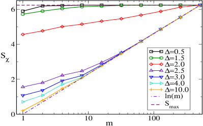
Figure 1: Variation of the observation entropy $S_{\chi}$ with coarse-graining length $m$ the middle spectrum states of the Hamiltonian $H$ for different values of $\Delta$.

First we focus on the eigenstates of the the Hamiltonian  (LABEL:nonint_model). For $\Delta=0$, the Hamiltonian ${H}$ can be easily diagonalized going into the momentum basis, i.e. ${H}(\Delta=0)=-2\sum_{k}\cos k{n}_{k}$, where $k=2n\pi/L$ with $n=0,1\cdot\cdot L-1$. The single-particle eigenvectors read as,

$$|\psi_{k}(\Delta=0)\rangle=\frac{1}{\sqrt{L}}\sum_{j=1}^{L}e^{ikj}{c}^{{\dagger}}_{j}|0\rangle.$$ (7)

We consider a pure state and ${\rho}=|\psi_{k}(\Delta=0)\rangle\langle\psi_{k}(\Delta=0)|$. In case of the finest coarse-graining, for which $V_{x_{1}}=1$, and for the ground state ($k=0$) $p_{x_{1}}=1/L$ for all $x_{1}$, which implies the observational entropy be simply equal to its Shannon entropy and $S_{\chi}=\ln L$. On the other hand, for the roughest coarse gaining $\chi_{I}\equiv x_{L}$, $S_{\chi}=\ln L$. By referring to the property represented by Eq. (3), for the ground state of the Hamiltonian ${H}(\Delta=0)$ , for any coarse gaining $S_{\chi}=\ln L$, maximal (see Fig. (1)). On the other hand, in the limit $\Delta\to\infty$, the eigenstates of the Hamiltonian ${H}$ are completely localized, they read as,

$$|\psi_{j_{0}}(\Delta\to\infty)\rangle={c}^{{\dagger}}_{j_{0}}|0\rangle,$$ (8)

where $j_{0}$ is the site index. Hence, $p_{x_{m}}=1$ only for a particular $x_{m}$ for which the site $j_{0}\in x_{m}$ and it is $0$ otherwise. It automatically implies, $S_{\chi}=\ln V_{x_{m}}$.

The change of the observational entropy with the coarse-graining length for the middle of the spectrum states are shown in the lower panel of Fig. (1) (we average over $10$ eigenstates from the middle of the spectrum around the energy $E\simeq 0$). For the delocalized phase, $\Delta<2$, observational entropy $S_{\chi}$ increases with the coarse-graining length and then it saturates to $S_{\text{max}}=\ln L$ for $m<L$. On the other hand, in the localized phase, $\Delta>2$, we find that beyond a certain coarse graning length $V_{x_{m}}=m>l_{c}$ ($l_{c}$ is some critical length scale depends on $\Delta$), $S_{\chi}=\ln V_{\chi}$.

In the localized phase, given the single particle wave function has the following form, $\psi(j)\simeq e^{-|j-j_{0}|/\xi}$ ($\xi$ is the localization length and $j_{0}$ is site at which the wave function has a peak), one expects that for coarse-graining length $m>2\xi$, $S_{\chi}=\ln V_{x_{m}}$. These observations can be clearly seen in figure. (1), where we find as $\Delta$ increases (localization length of the wavefunctions decrease), even for small values of coarse-graining length $S_{\chi}$ starts showing $\ln V_{x_{m}}$ scaling. However, it is worth pointing out that the growth of the $S_{\chi}$ as a function of $m$ in the delocalized phase much more rapid for the middle spectrum states compared to the ground state. While for the middle spectrum states $S_{\chi}=S_{\text{max}}=\ln L$ for $m<<L$, the ground state shows a slow logarithmic growth $S_{\chi}$ with coarse-graining size. This result is not very surprising given that typically one expects the degree of the delocalization (e.g. Shannon entropy) for high energy eigenstates to be much higher compared to the low energy ground state. Presumably, this fact gets reflected in the results.

IV.2 Dynamics

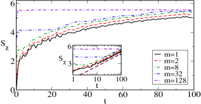
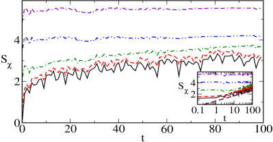
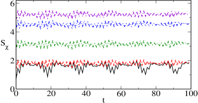
Figure 2: Variation of the observation entropy $S_{\chi}$ with time $t$ at the delocalized phase $\Delta=1$ (upper panel), transition point $\Delta=2$ (middle panel), and the localized phase $\Delta=3$ (lower panel) for different coarse-graining. Insets in the upper and middle panel shows logarithmic growth $S_{\chi}$ with $t$ for $m<<L$.

Here we study the behaviour of the observational entropy followed by the time evolution under the Hamiltonian $H$. We prepare the initial state such a way that electron is localized exactly on the middle of the lattice i.e., $|\psi(t=0)\rangle=|0_{1}0_{2}\cdot\cdot 1_{L/2}0_{L/2+1}...0_{L}\rangle$. The time-evolved state reads as,

$$|\psi(t)\rangle=e^{-iHt}|\psi(t=0)\rangle.$$ (9)

Given for $\Delta=0$ the Hamiltonian can be easily diagonalized in the momentum basis, and the time-evolved state at a given time can expressed as,

$$\psi(t,j)=\langle j|\psi(t)\rangle=\frac{1}{L}\sum_{k}e^{ikj+2it\cos k}.$$ (10)

In the thermodynamic limit, the series summation can be replaced by the integration. It is straight forward to check that observation entropy for the finest coarse-graining, i.e., $V_{x_{1}}=1$ will read as,

$$S_{\chi}=-2\sum_{j}(J_{j-L/2}(2t))^{2}\ln[J_{j-L/2}(2t)],$$ (11)

where $J_{k}()$ stands for Bessel function of 1st kind.

Numerically, in the thermodynamic limit (in Eqn. (11), by considering the summation over sufficiently large numbers of lattice sizes e.g. 256 or 512) the observational entropy in Eqn. (11) is $S_{\chi}\sim\ln t+\text{const}$. Hence, we expect to see $S_{\chi}\sim\ln t$ scaling for the systems we have studied here. Figure. (2) shows the variation of the observation entropy with time for different coarse-graining. In the delocalized phase, the electron which was initially localized in the middle of the lattice, will spread over both sides of the lattice, i.e., the probability of finding that electron on the other sites away from the middle of the lattice will also grow with time. It implies that the observational entropy $S_{\chi}$ will grow with time. That growth should be very apparent when $V_{x_{m}}<<L$. The upper panel of Fig. (2) shows that indeed for $V_{x_{m}}<<L$, the growth of $S_{\chi}\sim\ln t$ (see inset of Fig. (2) (upper panel)). This is precisely what we obtained analytically for $\Delta=0$ as well. Interestingly, even in the transition point i.e. $\Delta=2$, we find a similar logarithmic growth (with lower slope) of the observational entropy with time $S_{\chi}\sim 0.45\ln t$ (see the middle panel of Fig. 2). However, the slope is smaller than 1 what we found in the delocalized phase. This could be a consequence of the anomalous transport which has been found in this model at the transition point Purkayastha et al. (2018).

On the other hand, in the localized phase, as one can expect, the observation entropy does not show any growth, it shows oscillatory behavior (see lower panel of Fig. 2 for $\Delta=3$ results). Also, note that for the roughest graining i.e. $V_{x_{m}}=L$, $S_{\chi}(t)=\ln L$. Also, we find that for all time $S_{\chi}(t)\geq S_{\chi}(t=0)$ and $S_{\chi_{1}}(t)>S_{\chi_{2}}(t)$ where $\chi_{1}\hookrightarrow\chi_{2}$.

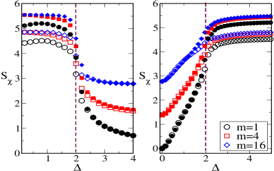
Figure 3: (Left panel)Variation of $S_{\chi}$ for the middle spectrum states of the Hamiltonian $H$ with $\Delta$ for different coarse-graining length $m$. (Right panel) Variation of $S_{\chi}$ for the middle spectrum states of the Hamiltonian $H$ with $\Delta$ for different momentum space coarse-graining length $m$. Results are for $L=128$ (inside empty symbols) and $L=256$ (inside filled symbols).

Next, we study the observation entropy as a function of $\Delta$ for different coarse-graining for different system size is shown in Fig. (3 (upper panel)). In the delocalized phase, $p_{x_{m}}\simeq V_{x_{m}}/L$, which implies $S_{\chi}\simeq\ln L$, hence $S_{\chi}$ increases with $L$. On the other hand, in the localized phase $S_{\chi}\simeq\ln V_{x_{m}}$, and does not depend on the system size as long as $V_{x_{m}}<L$. We also repeat the calculations for the momentum space coarse-graining, because of the self-dual property of the AA model one expects to see $S_{\chi}$ does not depend on $L$ for $\Delta<2$ (signature of localization) and $S_{\chi}$ increases with $L$ (signature of delocalization) for $\Delta>2$ (exactly opposite to what we had found in Fig. 3 (upper panel) for the real space coarse-graining). This is precisely what we observed in Fig. 3 (lower panel).

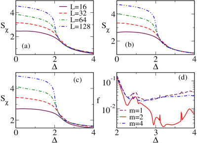
Figure 4: Variation of $S_{\chi}$ for the eigenstates of the Hamiltonian $H$ with $\Delta$ for coarse-graining (real space) length (a) $m=1$, (b) $m=2$, and (c) $m=3$ for $L=16$, 32, 64, 128. (d) Shows the variation of the fluctuation $f$ of $S_{\chi}$ with $\Delta$.

Figure. 3 clearly demonstrates that the observation entropy shows data collapse ( for different values of $L$) in the localized phase for any value of $m$ (as long as $m$ is smaller than the roughest coarse-graining length). However, for the finite size system, the question arises that how good is the data collapse. In contrast to the other diagnostic tools (e.g. Shannon entropy), observational entropy possesses an extra degree of freedom: the coarse-graining length. Hence, we calculate the normalized fluctuation, which is defined as,

$$f(\Delta,m)=\frac{\sqrt{\langle S_{\chi}^{2}\rangle-\langle S_{\chi}\rangle^{2}}}{\langle S_{\chi}\rangle}.$$ (12)

Here, $\langle\rangle$ stands for the average over different $L$ results. For the perfect data collapse, $f$ should be zero. On the other hand, the smaller the value of $f$, the better the data collapse. Figure. 4 shows the variation of $S_{\chi}$ with $\Delta$ for $m=1$, 2, 4. Looking at the figures, it is difficult to distinguish which coarse-graining length corresponds to better data collapse. Hence, we show the variation of $f$ with $\Delta$ in the localized region ($\Delta>2$). We find that $f$ is the minimum for $m=2$, which makes $m=2$ the optimal coarse-graining length for our case.

V Conclusions

Here we have studied the coarse-grained observational entropy for the 1D AA model, which supports localization-delocalization transition. First, we find that for the middle of spectrum states as one increases the coarse-grain size, the observational entropy very rapidly saturates to the upper bound i.e. $\ln L$. On the other hand, in the localized phase, typically if the coarse-grain size is greater than the order of localization length, the observational entropy increases as logarithmic of the coarse-grain size. Also, if the coarse-grain size is less than the system size, the observation entropy in the delocalized phase scales logarithmically with system size in contrast to the localized phase, where it does not depends on system size.

We have also investigated the fate of the observational entropy followed by a quantum quench under the AA Hamiltonian, where the particle was initially localized in the centre of the lattice. We found for a given coarse-graing (as long as the coarse-grain size is much smaller than the system time) in the delocalized phase (as well as in the localization-delocalization transition point), it grows with time logarithmically, while in the localized phase it does not grow at all. Finally, we also show that the observational entropy corresponding to the momentum space coarse-graining can clearly manifest the self-dual property of the AA model. We also have explicitly demonstrated that one can find an optimal coarse-graining length for which the finite size scaling shows much better data collapse.

While in this work, we had restricted our-self to the non-interacting systems, in the future work it will be interesting to investigate the behaviour of the observational entropy in the context of many-body localized systems, where the localization of many-body wave function takes place in the many-body fock space Ghosh et al. (2019); Sutradhar et al. (2022). As observational entropy is a directly measurable quantity, we would like to investigate the studies in the current paper in QC platforms.

VI Acknowledgements

RM acknowledges the DST-Inspire fellowship by the Department of Science and Technology, Government of India, SERB start-up grant (SRG/2021/002152). SA acknowledges the start-up research grant from SERB, Department of Science and Technology, Govt. of India (SRG/2022/000467). Authors thanks Vinod Rao, Ranjith V and Shaon Sahoo for fruitful discussions.

References

- von Neumann (2010) John von Neumann, “Proof of the ergodic theorem and the h-theorem in quantum mechanics,” The European Physical Journal H 35, 201–237 (2010).
- Shenker (1999) OR Shenker, “Is the entropy in quantum mechanics,” The British Journal for the Philosophy of Science 50, 33–48 (1999), http://bjps.oxfordjournals.org/content/50/1/33.full.pdf+html .
- Hemmo and Shenker (2006) Meir Hemmo and Orly Shenker, “Von neumann’s entropy does not correspond to thermodynamic entropy,” Philosophy of Science 73, 153–174 (2006).
- Mana et al. (2005) P. G. L. Mana, A. Maansson, and G. Bjoerk, “On distinguishability, orthogonality, and violations of the second law: contradictory assumptions, contrasting pieces of knowledge,” (2005), arXiv:quant-ph/0505229.
- Dahlsten et al. (2011) Oscar C O Dahlsten, Renato Renner, Elisabeth Rieper, and Vlatko Vedral, “Inadequacy of von neumann entropy for characterizing extractable work,” New Journal of Physics 13, 053015 (2011).
- Deville and Deville (2013) Alain Deville and Yannick Deville, “Clarifying the link between von neumann and thermodynamic entropies,” The European Physical Journal H 38, 57–81 (2013).
- Peres (1989) Asher Peres, “Nonlinear variants of schrödinger’s equation violate the second law of thermodynamics,” Phys. Rev. Lett. 63, 1114–1114 (1989).
- Weinberg (1989a) Steven Weinberg, “Precision tests of quantum mechanics,” Phys. Rev. Lett. 62, 485–488 (1989a).
- Weinberg (1989b) Steven Weinberg, “Weinberg replies,” Phys. Rev. Lett. 63, 1115–1115 (1989b).
- Hanggi and Wehner (2013) Esther Hanggi and Stephanie Wehner, “A violation of the uncertainty principle implies a violation of the second law of thermodynamics,” Nat Commun 4, 1670 (2013).
- Šafránek et al. (2021) Dominik Šafránek, Anthony Aguirre, Joseph Schindler, and JM Deutsch, “A brief introduction to observational entropy,” Foundations of Physics 51, 1–20 (2021).
- Šafránek et al. (2019a) Dominik Šafránek, J. M. Deutsch, and Anthony Aguirre, “Quantum coarse-grained entropy and thermodynamics,” Phys. Rev. A 99, 010101 (2019a).
- Šafránek et al. (2019b) Dominik Šafránek, J. M. Deutsch, and Anthony Aguirre, “Quantum coarse-grained entropy and thermalization in closed systems,” Phys. Rev. A 99, 012103 (2019b).
- (14) Carlton M. Caves, “Resource material for promoting the bayesian view of everything,” Personal notes.
- Gibbs (1902) Josiah Willard Gibbs, “Elementary principles in statistical mechanics: developed with especial reference to the rational foundations of thermodynamics,” (1902).
- Ehrenfest and Ehrenfest (1990) Paul Ehrenfest and Tatiana Ehrenfest, “The conceptual foundations of the statistical approach in mechanics,” (1990).
- Strasberg and Winter (2021) Philipp Strasberg and Andreas Winter, “First and second law of quantum thermodynamics: A consistent derivation based on a microscopic definition of entropy,” (2021), arXiv:2002.08817 [quant-ph] .
- Faiez et al. (2020) Dana Faiez, Dominik Šafránek, JM Deutsch, and Anthony Aguirre, “Typical and extreme entropies of long-lived isolated quantum systems,” Physical Review A 101, 052101 (2020).
- Šafránek et al. (2020) Dominik Šafránek, Anthony Aguirre, and JM Deutsch, “Classical dynamical coarse-grained entropy and comparison with the quantum version,” Physical Review E 102, 032106 (2020).
- Buscemi et al. (2022) Francesco Buscemi, Joseph Schindler, and Dominik Šafránek, “Observational entropy, coarse quantum states, and petz recovery: information-theoretic properties and bounds,” (2022).
- Schindler et al. (2020) Joseph Schindler, Dominik Šafránek, and Anthony Aguirre, “Quantum correlation entropy,” Physical Review A 102, 052407 (2020).
- PG et al. (2022) Sreeram PG, Ranjan Modak, and S Aravinda, “Witnessing quantum chaos using observational entropy,” arXiv preprint arXiv:2212.01585 (2022).
- Deutsch (2010) JM Deutsch, “Thermodynamic entropy of a many-body energy eigenstate,” New Journal of Physics 12, 075021 (2010).
- Deutsch et al. (2013) JM Deutsch, Haibin Li, and Auditya Sharma, “Microscopic origin of thermodynamic entropy in isolated systems,” Physical Review E 87, 042135 (2013).
- Santos et al. (2012) Lea F Santos, Anatoli Polkovnikov, and Marcos Rigol, “Weak and strong typicality in quantum systems,” Physical Review E 86, 010102 (2012).
- Georgescu et al. (2014) Iulia M Georgescu, Sahel Ashhab, and Franco Nori, “Quantum simulation,” Reviews of Modern Physics 86, 153 (2014).
- Altman et al. (2021) Ehud Altman, Kenneth R Brown, Giuseppe Carleo, Lincoln D Carr, Eugene Demler, Cheng Chin, Brian DeMarco, Sophia E Economou, Mark A Eriksson, Kai-Mei C Fu, et al., “Quantum simulators: Architectures and opportunities,” PRX Quantum 2, 017003 (2021).
- Serbyn et al. (2013) Maksym Serbyn, Z. Papić, and Dmitry A. Abanin, “Universal slow growth of entanglement in interacting strongly disordered systems,” Phys. Rev. Lett. 110, 260601 (2013).
- Iyer et al. (2013) Shankar Iyer, Vadim Oganesyan, Gil Refael, and David A. Huse, “Many-body localization in a quasiperiodic system,” Phys. Rev. B 87, 134202 (2013).
- Vidmar et al. (2018) Lev Vidmar, Lucas Hackl, Eugenio Bianchi, and Marcos Rigol, “Volume law and quantum criticality in the entanglement entropy of excited eigenstates of the quantum ising model,” Phys. Rev. Lett. 121, 220602 (2018).
- Vidmar and Rigol (2017) Lev Vidmar and Marcos Rigol, “Entanglement entropy of eigenstates of quantum chaotic hamiltonians,” Phys. Rev. Lett. 119, 220603 (2017).
- Vidmar et al. (2017) Lev Vidmar, Lucas Hackl, Eugenio Bianchi, and Marcos Rigol, “Entanglement entropy of eigenstates of quadratic fermionic hamiltonians,” Phys. Rev. Lett. 119, 020601 (2017).
- Vosk and Altman (2013) Ronen Vosk and Ehud Altman, “Many-body localization in one dimension as a dynamical renormalization group fixed point,” Phys. Rev. Lett. 110, 067204 (2013).
- Bardarson et al. (2012) Jens H. Bardarson, Frank Pollmann, and Joel E. Moore, “Unbounded growth of entanglement in models of many-body localization,” Phys. Rev. Lett. 109, 017202 (2012).
- Abanin et al. (2019) Dmitry A. Abanin, Ehud Altman, Immanuel Bloch, and Maksym Serbyn, “Colloquium: Many-body localization, thermalization, and entanglement,” Rev. Mod. Phys. 91, 021001 (2019).
- Islam et al. (2015) Rajibul Islam, Ruichao Ma, Philipp M Preiss, M Eric Tai, Alexander Lukin, Matthew Rispoli, and Markus Greiner, “Measuring entanglement entropy in a quantum many-body system,” Nature 528, 77–83 (2015).
- Carr et al. (2009) Lincoln D Carr, David DeMille, Roman V Krems, and Jun Ye, “Cold and ultracold molecules: science, technology and applications,” New Journal of Physics 11, 055049 (2009).
- Safronova et al. (2018) MS Safronova, D Budker, D DeMille, Derek F Jackson Kimball, A Derevianko, and Charles W Clark, “Search for new physics with atoms and molecules,” Reviews of Modern Physics 90, 025008 (2018).
- Atatüre et al. (2018) Mete Atatüre, Dirk Englund, Nick Vamivakas, Sang-Yun Lee, and Joerg Wrachtrup, “Material platforms for spin-based photonic quantum technologies,” Nature Reviews Materials 3, 38–51 (2018).
- Vandersypen and Eriksson (2019) Lieven MK Vandersypen and Mark A Eriksson, “Quantum computing with semiconductor spins,” Physics Today 72, 8–38 (2019).
- Hensgens et al. (2017) Toivo Hensgens, Takafumi Fujita, Laurens Janssen, Xiao Li, CJ Van Diepen, Christian Reichl, Werner Wegscheider, Sankar Das Sarma, and Lieven MK Vandersypen, “Quantum simulation of a fermi–hubbard model using a semiconductor quantum dot array,” Nature 548, 70–73 (2017).
- Hartmann et al. (2008) Michael J Hartmann, Fernando GSL Brandao, and Martin B Plenio, “Quantum many-body phenomena in coupled cavity arrays,” Laser & Photonics Reviews 2, 527–556 (2008).
- Vaidya et al. (2018) Varun D Vaidya, Yudan Guo, Ronen M Kroeze, Kyle E Ballantine, Alicia J Kollár, Jonathan Keeling, and Benjamin L Lev, “Tunable-range, photon-mediated atomic interactions in multimode cavity qed,” Physical Review X 8, 011002 (2018).
- Norcia et al. (2018) Matthew A Norcia, Robert J Lewis-Swan, Julia RK Cline, Bihui Zhu, Ana M Rey, and James K Thompson, “Cavity-mediated collective spin-exchange interactions in a strontium superradiant laser,” Science 361, 259–262 (2018).
- Davis et al. (2019) Emily J Davis, Gregory Bentsen, Lukas Homeier, Tracy Li, and Monika H Schleier-Smith, “Photon-mediated spin-exchange dynamics of spin-1 atoms,” Physical review letters 122, 010405 (2019).
- Wang et al. (2015) Da-Wei Wang, Han Cai, Luqi Yuan, Shi-Yao Zhu, and Ren-Bao Liu, “Topological phase transitions in superradiance lattices,” Optica 2, 712–715 (2015).
- Noh and Angelakis (2016) Changsuk Noh and Dimitris G Angelakis, “Quantum simulations and many-body physics with light,” Reports on Progress in Physics 80, 016401 (2016).
- Hartmann (2016) Michael J Hartmann, “Quantum simulation with interacting photons,” Journal of Optics 18, 104005 (2016).
- Kjaergaard et al. (2020) Morten Kjaergaard, Mollie E Schwartz, Jochen Braumüller, Philip Krantz, Joel I-J Wang, Simon Gustavsson, and William D Oliver, “Superconducting qubits: Current state of play,” Annual Review of Condensed Matter Physics 11, 369–395 (2020).
- Ganzhorn et al. (2019) Marc Ganzhorn, Daniel J Egger, Panagiotis Barkoutsos, Pauline Ollitrault, Gian Salis, Nikolaj Moll, Marco Roth, A Fuhrer, P Mueller, Stefan Woerner, et al., “Gate-efficient simulation of molecular eigenstates on a quantum computer,” Physical Review Applied 11, 044092 (2019).
- Kandala et al. (2017) Abhinav Kandala, Antonio Mezzacapo, Kristan Temme, Maika Takita, Markus Brink, Jerry M Chow, and Jay M Gambetta, “Hardware-efficient variational quantum eigensolver for small molecules and quantum magnets,” Nature 549, 242–246 (2017).
- Hempel et al. (2018) Cornelius Hempel, Christine Maier, Jonathan Romero, Jarrod McClean, Thomas Monz, Heng Shen, Petar Jurcevic, Ben P Lanyon, Peter Love, Ryan Babbush, et al., “Quantum chemistry calculations on a trapped-ion quantum simulator,” Physical Review X 8, 031022 (2018).
- Nam et al. (2020) Yunseong Nam, Jwo-Sy Chen, Neal C Pisenti, Kenneth Wright, Conor Delaney, Dmitri Maslov, Kenneth R Brown, Stewart Allen, Jason M Amini, Joel Apisdorf, et al., “Ground-state energy estimation of the water molecule on a trapped-ion quantum computer,” npj Quantum Information 6, 1–6 (2020).
- Britton et al. (2012) Joseph W Britton, Brian C Sawyer, Adam C Keith, C-C Joseph Wang, James K Freericks, Hermann Uys, Michael J Biercuk, and John J Bollinger, “Engineered two-dimensional ising interactions in a trapped-ion quantum simulator with hundreds of spins,” Nature 484, 489–492 (2012).
- Bohnet et al. (2016) Justin G Bohnet, Brian C Sawyer, Joseph W Britton, Michael L Wall, Ana Maria Rey, Michael Foss-Feig, and John J Bollinger, “Quantum spin dynamics and entanglement generation with hundreds of trapped ions,” Science 352, 1297–1301 (2016).
- Aubry and André (1980) Serge Aubry and Gilles André, “Analyticity breaking and anderson localization in incommensurate lattices,” Ann. Israel Phys. Soc 3, 18 (1980).
- Anderson (1958) Philip W Anderson, “Absence of diffusion in certain random lattices,” Physical review 109, 1492 (1958).
- Abrahams et al. (1979) Elihu Abrahams, PW Anderson, DC Licciardello, and TV Ramakrishnan, “Scaling theory of localization: Absence of quantum diffusion in two dimensions,” Physical Review Letters 42, 673–676 (1979).
- Lee and Ramakrishnan (1985) Patrick A Lee and TV Ramakrishnan, “Disordered electronic systems,” Reviews of Modern Physics 57, 287 (1985).
- Kaufman et al. (2016) Adam M Kaufman, M Eric Tai, Alexander Lukin, Matthew Rispoli, Robert Schittko, Philipp M Preiss, and Markus Greiner, “Quantum thermalization through entanglement in an isolated many-body system,” Science 353, 794–800 (2016).
- Note (1) Since we are concerned on studying observational entropy, unless otherwise specified, denotes observational entropy and we don’t use subscript/superscript to denote observational entropy. Other type of entropies are denoted with suitable subscripts.
- Purkayastha et al. (2018) Archak Purkayastha, Sambuddha Sanyal, Abhishek Dhar, and Manas Kulkarni, “Anomalous transport in the aubry-andré-harper model in isolated and open systems,” Phys. Rev. B 97, 174206 (2018).
- Ghosh et al. (2019) Soumi Ghosh, Atithi Acharya, Subhayan Sahu, and Subroto Mukerjee, “Many-body localization due to correlated disorder in fock space,” Phys. Rev. B 99, 165131 (2019).
- Sutradhar et al. (2022) Jagannath Sutradhar, Soumi Ghosh, Sthitadhi Roy, David E. Logan, Subroto Mukerjee, and Sumilan Banerjee, “Scaling of the fock-space propagator and multifractality across the many-body localization transition,” Phys. Rev. B 106, 054203 (2022).