Evaluating Continuous Basic Graph Patterns over Dynamic Link Data Graphs

Abstract

In this paper, we investigate the problem of evaluating Basic Graph Patterns (BGP, for short, a subclass of SPARQL queries) over dynamic Linked Data graphs; i.e., Linked Data graphs that are continuously updated. We consider a setting where the updates are continuously received through a stream of messages and support both insertions and deletions of triples (updates are straightforwardly handled as a combination of deletions and insertions). In this context, we propose a set of in-memory algorithms minimizing the cached data for efficiently and continuously answering main subclasses of BGP queries. The queries are typically submitted into a system and continuously result the delta answers while the update messages are processed. Consolidating all the historical delta answers, the algorithms ensure that the answer of each query is constructed at any given time.

1 Introduction

The dynamic graphs describe graphs that are continuously modified over time, usually, through a stream of edge updates (insertions and deletions). Representative examples include social graphs [balduini2015citysensing], traffic and transportation networks [lecue2012capturing], [tallevi2013real], financial transaction networks [schneider2012microsecond], and sensor networks [sheth2008semantic]. When the graph data is rapidly updated, conventional graph management systems are not able to handle high velocity data in a reasonable time. In such cases, real-time query answering becomes a major challenge.

RDF data model and Linked Data paradigm are widely used to structure and publish semantically-enhanced data. The last decades, both private and public organizations have been more and more following this approach to disseminate their data. Due to the emergence and spread of IoT, such an approach attracted further attention from both industry and research communities. To query such type of data, SPARQL is a standard query language that is widely used.

Querying streaming Linked Data has been extensively investigated in the literature, where the majority of the related work [dell2017stream, margara2014streaming] focus on investigating frameworks for efficiently querying streaming data; mainly focusing on defining certain operators for querying and reasoning data in sliding windows (i.e., predefined portion of the streaming data). In this work, we mainly focus on efficiently handling the continuously updated Linked Data graph (i.e., Dynamic Link Data Graphs). In particular, we consider a setting where the updates are continuously received through a stream of messages and support both insertions and deletions of triples (updates are straightforwardly handled as a combination of deletions and insertions). In this context, we propose a set of in-memory algorithms minimizing the cached data for efficiently and continuously answering main subclasses of Basic Graph Patterns (BGP, for short, a subclass of SPARQL queries). The queries are typically submitted into a system and continuously result the delta answers while the update messages are processed. The evaluation approach is based on applying an effective decomposition of the given queries in order to both improve the performance of query evaluation and minimize the cached data. Consolidating all the historical delta answers, the algorithms ensure that the answer of each query is constructed at any given time.

The paper is structured as follows. Section 2 presents the related work. The main concepts and definitions used throughout this work are formally presented in Section 3. Section 4 focus on defining main subclasses of BGP queries, while the problem, along with the relevant setting, investigated in work are formally defined in Section 5. Section 6 includes the main contributions of this work; i.e., the query answering algorithms applied over the dynamic Linked Data graphs. Finally, we conclude in Section LABEL:sec:conclusion.

2 Related work

The problem of querying and detecting graph patterns over streaming RDF and Linked Data has been extensively investigated in the literature [dell2017stream, margara2014streaming]. In this context, there have been proposed and analysed multiple settings, such as Data Stream Management Systems (DSMS - e.g., [BarbieriBCVG10, BarbieriBCG10, le2011native, jesper2011high, bolles2008streaming]), and Complex Event Processing Systems (CEP - e.g., [GroppeGKL07, anicic2011ep, roffia2018dynamic, PhamAM19, gillani2016continuous]).

In DSMSs, the streaming data is mainly represented by relational messages and the queries are translated into plans of relational operators. Representative DSMS systems are the following: C-SPARQL [BarbieriBCVG10, BarbieriBCG10], CQELS [le2011native], C-SPARQL on S4 [jesper2011high] and Streaming-SPARQL [bolles2008streaming]. The majority of the DSMS approaches use sliding windows to limit the data and focus on proposing a framework for querying the streaming data included in the window. In addition, they mainly use relational-like operators which are evaluated over the data included in the window. Note that this type of systems mainly focus on querying the data into windows and do not focus on setting up temporal operators.

On the other hand, CEP systems follow a different approach. These approaches handle the streaming data as an infinite sequence of events which are used to compute composite events. EP-SPARQL [anicic2011ep] is a representative system of this approach, which defines a language for event processing and reasoning. It also supports windowing operators, as well as temporal operators. C-ASP [PhamAM19], now, is a hybrid approach combining the windowing mechanism and relational operators from DSMS systems, and the rule-based and event-based approach of CEP systems.

In the aforementioned approaches the streaming data mainly include new triples; i.e., no deletion of graph triples is considered, as in the setting investigated in this paper. Capturing updates (including deletion delivered by the stream) of the streaming data has been investigated in the context of incremental reasoning (e.g., [ren2011optimising, dell2014ch, barbieri2010incremental, volz2005incrementally, volz2005incrementally]). Incremental Materialization for RDF STreams (IMaRS) [dell2014ch, barbieri2010incremental] considers streaming input annotated with expiration time, and uses the processing approach of C-SPARQL. Ren et al. in [ren2011optimising, ren2010towards], on the other hand, focuses on more complex ontology languages, and does not considers fixed time windows to estimate the expiration time.

The concept of expiration time is also adopted in [choi2018efficient] for computing subgraph matching for sliding windows. The authors also use a query decomposition approach based on node degree in graph streams. Fan et al. in [fan2013incremental] investigated the incremental subgraph matching by finding a set of differences between the original matches and the new matches. In [CHC+15], the authors used a tree structure where the root node contains the query graph and the other nodes include subqueries of it. The leaf nodes of this structure include the edges of the query, and the structure is used to incrementally apply the streaming changes (partial matches are also maintained). In the same context, Graphflow [kankanamge2017graphflow] and TurboFlux [kim2018turboflux] present two approaches for incremental computation of delta matches. Graphflow [kankanamge2017graphflow] is based on a worst-case optimal join algorithm to evaluate the matching for each update, while TurboFlux [kim2018turboflux] extends the input graph with additional edges, taking also into account the form of the query graph. This structure is used to efficiently find the delta matches.

3 Preliminaries

In this section, we present the basic concepts used throughout this work.

3.1 Data and query graphs

Initially, we define two types of directed, labeled graphs with labeled edges that represent RDF data and Basic Graph Patterns (i.e., a subclass of SPARQL) over the RDF data. In the following, we consider two disjoint infinite sets $U_{so}$ and $U_{p}$ of URI references, an infinite set of (plain) literals $L$ and a set of variables $V$.

A data triple is a triple of the form $(s,p,o)$, where $s$ take values from $U_{so}$, $o$ takes values from $(U_{so}\cup L)$ and $p$ takes values from $U_{p}$; i.e., $(s,p,o)\in U_{so}\times U_{p}\times(U_{so}\cup L)$. In each triple of this form, we say that $s$ is the subject, $p$ is the predicate and $o$ is the object of $t$. A data graph $G$ is defined as a non-empty set of data triples. Similarly, we define a query triple pattern (query triple for short) as a triple $(s,p,o)$ in $(U_{so}\cup V)\times U_{p}\times(U_{so}\cup L\cup V)$; i.e., $s$ could be either URI or variables from $V$ and $o$ could be either URI or variable, or literal. A Basic Graph Pattern (BGP), or simply a query (graph), $Q$ is defined as a non-empty set of query triple patterns. In essence, each triple $(s,p,o)$ in the query and data graphs represents a directed edge from $s$ to $o$ which is labeled by $p$, while $s$ and $o$ represent nodes in the corresponding graphs. The output pattern $O(Q)$ of a query graph $Q$ is the tuple $(X_{1},\dots,X_{n})$, with $n\geq 0$, of all the variables appearing in $Q$ w.r.t. to a total order over the variables of $Q$ . A query $Q$ is said to be a Boolean, or ground, query if $n=0$ (i.e., there is not any variable in $Q$). The set of nodes of a data graph $G$ (resp. query graph $Q$) is denoted as ${\cal N}(G)$ (resp. ${\cal N}(Q)$). The set of variables of $Q$ is denoted as ${\cal V}(Q)$. In the following, we refer to either a URI or literal node as constant node. Furthermore, we say that a data graph (resp. query graph $Q$) $G^{\prime}$ is a subgraph of a data (resp. query) graph $G$ if $G^{\prime}\subseteq G$.

3.2 Data and query graph decomposition

In this subsection we define the notion of data and query graph decomposition.

Definition 1

A data (resp. query) graph decomposition ${\cal D}(F)$ of a data (resp. query) graph $F$ is an $m$-tuple of data (resp. query) graphs ${\cal D}(F)=(F_{1},\dots,F_{m})$, with $m\geq 1$, such that:

1. $F_{i}\subseteq F$, for $i=1,\dots,m$, and

2. $\bigcup_{i}F_{i}=F$.

Each data (resp. query) graph $F_{i}$ in a data (resp. query) graph decomposition is called a data (resp. query) graph segment. When, in a data/query graph decomposition, for all pairs $i$, $j$, with $1\leq i<j\leq m$, it also holds $F_{i}\cap F_{j}=\emptyset$, i.e. data (resp. query) graph segments are disjoint of each other, then the data (resp. query) graph decomposition is said to be non-reduntant and the graph (resp. query) segments obtained form a partition of the triples of data (resp. query) graph $F$, called $m$-triple partition of $F$.

3.3 Embeddings and query answers

This subsection focuses on describing the main concepts used for the query evaluation. To compute the answers of a query $Q$ when it is posed on a data graph G, we consider finding proper mappings from the nodes and edges of $Q$ to the nodes and edges of $G$. Such kind of mappings are described by the concept of embedding, which is formally defined as follows.

Definition 2

A (total) embedding of a query graph $Q$ in a data graph $G$ is a total mapping $e:{\cal{N}}(Q)\rightarrow{\cal{N}}(G)$ with the following properties:

1. For each node $v\in{\cal{N}}(Q)$, if $v$ is not a variable then $v=e(v)$.

2. For each triple $(s,p,o)\in Q$, the triple $(e(s),p,e(o))$ is in $G$.

The tuple $(e(X_{1}),\dots,e(X_{n}))$, where $(X_{1},\dots,X_{n})$ is the output pattern of $Q$, is said to be an answer to the query $Q$. Notice that $e(Q)\subseteq G$. The set containing the answers of a query $Q$ over a graph $G$ is denoted as $Q(G)$.

Note that the variables mapping [perez2008semantics, perez2009semantics] considered for SPARQL evaluation is related with the concept of the embedding as follows. If $Q$ is a query pattern and $G$ is a data graph, and there is an embedding $e$ from ${\cal N}(Q)$ to ${\cal N}(G)$, then the mapping $\mu$ from ${\cal V}(Q)$ to ${\cal N}(G)$, so that $e(n)=\mu(n)$ for each variable node $n$ in ${\cal V}(Q)$, is a variable mapping.

Definition 3

A partial embedding of a query graph $Q$ in a data graph $G$ is a partial mapping $e:{\cal{N}}(Q)\rightarrow{\cal{N}}(G)$ with the following properties:

1. For each node $v\in{\cal{N}}(Q)$ for which $e(v)$ is defined, if $v$ is not a variable then $v=e(v)$.

2. For each triple $(s,p,o)\in Q$, for which both $e(s)$ and $e(o)$ are defined, the triple $(e(s),p,e(o))$ is in $G$.

In essence, a partial embedding represents a mapping from a subset of nodes and edges of a query $Q$ to a given data graph $G$. In other words, partial embeddings represent partial answers to $Q$, provided that, they can be appropriately “combined" with other “compatible" partial embeddings to give “complete answers” (i.e. total embeddings) to the query $Q$.

Definition 4

Two partial mappings $e_{1}:D_{1}\rightarrow R_{1}$ and $e_{2}:D_{2}\rightarrow R_{2}$ are said to be compatible if for every node $v\in{\cal{N}}(D_{1})\cap{\cal{N}}(D_{2})$ such that $e_{1}(v)$ and $e_{2}(v)$ are defined, it holds that $e_{1}(v)=e_{2}(v)$.

Definition 5

Let $e_{1}:D_{1}\rightarrow R_{1}$ and $e_{2}:D_{2}\rightarrow R_{2}$ be two compatible partial mappings. The join of $e_{1}$ and $e_{2}$, denoted as $e_{1}\otimes e_{2}$, is the partial mapping $e:D_{1}\cup D_{2}\rightarrow R_{1}\cup R_{2}$ defined as follows:

$$e(v)=\left\{\begin{array}[]{ll}e_{1}(v)&\mbox{if $e_{1}(v)$ is defined}\\ e_{2}(v)&\mbox{if $e_{2}(v)$ is defined and $e_{1}(v)$ is undefined}\\ \textup{undefined}&\mbox{if both $e_{1}(v)$ and $e_{2}(v)$ are undefined}\\ \end{array}\right.$$

4 Special forms of queries and query decomposition

4.1 Special forms of queries

We now define two special classes of queries, the generalized star queries (star queries, for short) and the queries with connected-variables (var-connected queries, for short).

Definition 6

A query $Q$ is called a generalized star query if there exists a node $c\in{\cal N}(Q)$, called the central node of $Q$ and denoted as $C(Q)$, such that for every triple $t=(s,p,o)\in Q$ it is either $s=c$ or $o=c$. If the central node of $Q$ is a variable then $Q$ is called var-centric generalized star query. A var-centric star query is simple if all the adjacent nodes to the central node are constants.

To define the class of var-connected queries we first define the notion of generalized path connecting two nodes of the query $Q$.

Definition 7

Let $Q$ be a BGP query and $v_{1}$, $v_{k+1}$, with $k\geq 1$, be two nodes in $Q$. A generalized path between $v_{1}$ and $v_{k+1}$ of length $k$, is a sequence of triples $t_{1},\dots,t_{k}$ such that:

1. there exists a sequence of nodes $v_{2}$, $\dots$, $v_{k}$ in $Q$, where $v_{1},v_{2},\dots,v_{k},v_{k+1}$ are disjoint, and a sequence of predicates $p_{1},\dots,p_{k}$ not necessarily distinct, and

2. for each $i$, with $1\leq i\leq k$, either $t_{i}=(v_{i},p_{i},v_{i+1})$, or $t_{i}=(v_{i+1},p_{i},v_{i})$.

The distance $d(v,v^{\prime})$ between two nodes $v$ and $v^{\prime}$ in $Q$, is the length of (i.e. the number of triples in) the shortest generalized path between $v$ and $v^{\prime}$.

Definition 8

Consider now a BGP query $Q$ with multiple variables (i.e., $|{\cal V}(Q)|>1$) such that for each pair of variables $(X,Y)$ of $Q$ there is a generalized path connecting $X$ and $Y$ which does not contain any constant. In such a case, we say that $Q$ is a var-connected query.

Notice that a var-centric query which is not simple is var-connected query.

4.2 Connected-variable partition of BGP queries

In this section we present a decomposition of BGP queries called connected-variable partition of a BGP query. Connected-variable partition is a non-redundant decomposition of a BGP query $Q$ into a set of queries whose form facilitates, as we will see in subsequent sections, their efficient evaluation over a dynamic Linked Datagraph.

Definition 9

Let $Q$ be a BGP query and $V$ be the set of variables in $Q$. A partition ${\cal P}(V)$ of the variables in $V$, is said to be a connected-variable partition of $V$ if the following hold:

1. For each $P_{i}\in{\cal P}(V)$ and for every two disjoint variables $u,v\in P_{i}$, there is a generalized path between $u$ and $v$ in $Q$ whose nodes are variables belonging to $P_{i}$.

2. For each pair $P_{i},P_{j}\in{\cal P}(V)$, with $i\neq j$, there is no pair of variables $u$, $v$ such that $u\in P_{i}$ and $v\in P_{j}$ and there is a triple in $Q$ whose subject is one of these variables and whose object is the other.

Definition 10

Let $Q$ be a BGP query, $V$ be the set of variables in $Q$, and ${\cal P}(V)$ be the connected-variable partition of $V$. The connected-variable decomposition ${\cal D_{CV}}(Q)$ of $Q$ is a non-redundant decomposition of $Q$ containing $|{\cal P}(V)|$ non-ground queries (i.e. queries containing variables), and (possibly) a ground query $Q_{G}$. These queries are constructed as follows:

1. For each element $P_{i}\in{\cal P}(V)$, we construct a query $Q_{P_{i}}$ = $\{t|t=(s,p,o)\in Q$ and either $s\in P_{i}$ or $o\in P_{i}\}$.

2. $Q_{G}=Q-\bigcup_{i}Q_{P_{i}}$.

Note that $Q_{G}$ may be empty. In this case $Q_{G}$ is not included in ${\cal D_{CV}}(Q)$. Notice also that when, for some $i$, it holds that $|P_{i}|=1$, then $Q_{P_{i}}$ is a simple var-centric star query.

Example 1

Consider the query $Q$ appearing in Fig. 1. The set of variables of $Q$ is $V=\{?X,?Y,?Z,?W\}$, while the connected-variables partition ${\cal P}(V)$ of $V$ is ${\cal P}(V)=\{\{?X,?Y,?Z\},\{?W\}\}$. The connected variable decomposition ${\cal D_{CV}}(Q)$ of $Q$ is ${\cal D_{CV}}(Q)=\{Q_{1},Q_{2},Q_{G}\}$. $Q_{1}$, $Q_{2}$ and $Q_{G}$ also appear in Fig. 1.

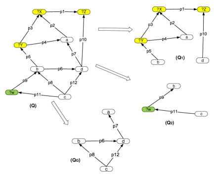
Figure 1: Connected-variable decomposition of a BGP query $Q$.

It should be noted that, under certain conditions, i.e. when all members of ${\cal P}(V)$ are singletons, all queries in ${\cal D_{CV}}(Q)$ containing variables may be in the form of simple var-centric star queries.

Definition 11

A BGP query $Q$ is said to be loosely-connected if for each pair of disjoint variables $X$, $Y$ in $Q$, it holds that every generalized path between $X$ and $Y$ contains at least one non-variable node.

Lemma 1

Let $Q$ be a loosely-connected BGP query and ${\cal D_{CV}}(Q)$ be the connected variable decomposition of $Q$. Then each non-ground query in ${\cal D_{CV}}(Q)$ is a simple var-centric star query.

Proof

From Definitions 9 and 11, we conclude that each member of the connected-variable partition ${\cal P}(V)$ of the set of variables $V$ of a loosely-connected BGP query $Q$ is singleton. As the queries in ${\cal D_{CV}}(Q)$ are obtained by applying Definition 10, we see that, by construction, each query in ${\cal D_{CV}}(Q)$ has a variable as a central node which is either the subject or the object of triples which have a non-variable object or subject, respectively. Based on Definition 6, we conclude that these queries are simple var-centric star queries.  

Example 2

Consider the BGP query $Q$ appearing in Fig. 2. The set of variables of $Q$ is $V=\{?X,?Y,?Z\}$, while the connected-variables partition ${\cal P}(V)$ of $V$ is ${\cal P}(V)=\{\{?X\},\{?Y\},\{?Z\}\}$. The connected variable decomposition ${\cal D_{CV}}(Q)$ of $Q$ is ${\cal D_{CV}}(Q)=\{Q_{1}$, $Q_{2}$, $Q_{3}$, $Q_{G}\}$, where $Q_{1}$, $Q_{2}$, $Q_{3}$, and $Q_{G}$ appear in Fig. 2. We can see that each query containing variables (i.e. $Q_{1}$, $Q_{2}$, and $Q_{3}$) is a simple var-centric star query.

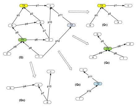
Figure 2: Connected-variable decomposition of a loosely connected BGP query $Q$.

Definition 12

Let $Q$ be a BGP query and $V$ be the set of variables in $Q$. Assume that $|V|\geq 2$ and ${\cal P}(V)$ is the connected-variable partition of $V$. Then, if ${\cal P}(V)$ is a singleton, we say that $Q$ is a connected-variable query.

5 Continuous pattern matching

The main challenge we are investigating in this work is the case where the data graph is continuously changing (a.k.a, dynamic data graph), through an infinite sequence of updates over the data.

In particular, we initially consider an infinite, ordered sequence ${\cal M}$ $=$ $({\cal U}_{1}$, ${\cal U}_{2}$, $\dots)$ of update messages, called update stream, of the form ${\cal U}_{k}=<t_{k},Op,e>$, where

• $t_{k}$ is the time the message received, where $k=1,2,\dots$,

• $Op$ is an update operation applied over a data graph and takes values from the following domain: $\{ins$, $del\}$, and

• $e=(s,p,o)$ is the edge to be either inserted or deleted (according to the operation specified by $Op$).

Note that the $ins$ operation stands for $insertion$, while $del$ stands for $deletion$. For example, the message $<t,ins,(s,p,o)>$, which is received at time $t$ describes an insertion of the edge $(s,p,o)$ into the data graph. The data graph resulted by applying an update message ${\cal U}_{k}$ in ${\cal M}$ over a data graph $G$ is a data graph ${\cal U}_{k}(G)$ defined as follows:

$${\cal U}_{k}(G)=\left\{\begin{array}[]{ll}G\cup\{(s,p,o))\},&\quad O=ins\\ G-\{(s,p,o)\},&\quad O=del\end{array}\right.$$

Suppose, now, a data graph $G_{0}$ at a certain time $t_{0}$. At time $t_{1}$, we receive an update message ${\cal U}_{1}$ in ${\cal M}$. Applying the update ${\cal U}_{1}$ on $G_{0}$, we get an updated graph $G_{1}$. Similarly, once we receive the update message ${\cal U}_{2}$ in ${\cal M}$ and apply it into $G_{1}$, we get the graph $G_{2}$. Continuously applying all the updates that are being received through ${\cal M}$, we have a data graph that is slightly changing over time. We refer to such a graph $G=(G_{0},G_{1},\dots,G_{k},\dots)$ as dynamic graph, and to each data graph at a certain time as snapshot of $G$. For simplicity, we denote the snapshot of $G$ at time $t_{k}$ as $G(t_{k})$. Hence, at time $t_{k}$, the graph snapshot $G_{k}$ of $G$ is given as follows:

$${\cal U}_{[0..k]}(G_{0})=G_{k}={\cal U}_{k}(G_{k-1})={\cal U}_{k}({\cal U}_{k-1}(\dots{\cal U}_{1}(G_{0})\dots))$$

Considering a BGP query $Q$ which is continuously applied on each snapshot of the dynamic graph $G=(G_{0},G_{1},\dots,G_{k},\dots)$, we might find different results at each time the query is evaluated. In particular, if $G_{k-1}$ is the graph snapshot at time $t_{k-1}$ and we receive an insertion message at time $t_{k}$, $Q(G_{k})$ might contain embeddings that were not included in $Q(G_{k-1})$. In such a case (i.e., if $Q(G_{k})\supset Q(G_{k-1})$), we say that each embedding in $Q(G_{k})-Q(G_{k-1})$ is a positive embedding. Similarly, if we consider that the message received at time $t_{k}$ is a deletion, we might have embeddings in $Q(G_{k-1})$ that are no longer valid in $Q(G_{k})$ (i.e., $Q(G_{k})\subset Q(G_{k-1})$). If so, each embedding in $Q(G_{k-1})-Q(G_{k})$ is called negative embedding. For simplicity, we refer to the set of positive and negative embeddings at time $t_{k}$ as delta embeddings. In the following, we denote the sets of positive, negative and delta embeddings, at time $t_{k}$, as $Q^{+}(G_{k})$, $Q^{-}(G_{k})$ and $Q^{\delta}(G_{k})$, respectively.

Let us now formally define the problem of continuous pattern matching.

Definition 13

(Problem Definition) Considering a dynamic graph $G=(G_{0},G_{1},\dots,G_{k},\dots)$, an update stream ${\cal M}=({\cal U}_{1},{\cal U}_{2},\dots)$, and a query $Q$, we want to find for each time $t_{k}$, with $k=1,2,\dots$, the outputs of all the delta embeddings $Q^{\delta}(G_{k})=Q^{+}(G_{k})\cup Q^{-}(G_{k})$, where

• $G_{k}={\cal U}_{[0..k]}(G_{0})$,

• the positive embeddings is given as $Q^{+}(G_{k})=Q(G_{k})-Q(G_{k-1})$,

• the negative embeddings is given as $Q^{-}(G_{k})=Q(G_{k-1})-Q(G_{k})$.

The following sections are based on the following assumptions:

• Whenever an update message of the form $<t_{k},del,e>$ is received, we assume that $e\in G_{k-1}$.

• Whenever an update message of the form $<t_{k},ins,e>$ is received, we assume that $e\notin G_{k-1}$.

6 Answering BGP queries over dynamic Linked Data

In this section, we investigate methods for continuously answering BGP queries over dynamic graphs. In particular, we focus on finding the delta embeddings for each message received from an update stream. The set of embeddings found by each of the algorithms presented in the subsequent sections ensure that collecting all the delta embeddings from the beginning of the stream to the time $t$ and applying the corresponding operations (deletions and insertions) according to the order they found, the remaining embeddings describe the answer of the given query over the graph $G_{t}$. We focus on certain well-used subclasses of BGP queries, defined in the previous sections, which include ground BGP queries, simple var-centric star queries, and loosely-connected BGP queries. In addition, we present a sketch for generalizing our algorithms for connected-variable queries.

6.1 A generic procedure employing the connected-variable partition of a query

Starting our analysis, we initially focus on the intuition of the evaluation algorithms presented in the subsequent section. The methodology used to construct the algorithms relies on the proper decomposition of the given query into a set of subqueries. The following lemma shows that finding a connected-variable decomposition of a query, the total embeddings of the subqueries give a total embedding of the initial query.

Lemma 2

Let $G$ be a data graph and $Q$ be a BGP query. Assume that ${\cal D_{CV}}(Q)$ = $\{Q_{1},Q_{2},\dots,Q_{n}\}$ is the connected-variable decomposition of $Q$. Assume also that $e_{1},e_{2},\dots,e_{n}$ are total embeddings of $Q_{1},Q_{2},\dots,Q_{n}$ respectively, in $G$. Then, $e_{1},e_{2},\dots,e_{n}$ are compatible partial embeddings of $Q$ in $G$ and $e=e_{1}\otimes e_{2}\otimes\dots\otimes e_{n}$ is a total embedding of $Q$ in $G$.