Viscosity approximation method for a variational problem

Abstract.

Let $Q$ be a nonempty closed and convex subset of a real Hilbert space $\mathcal{H}$, $S:Q\rightarrow Q$ a nonexpansive mapping, $A:Q\rightarrow Q$ an inverse strongly monotone operator, and $f:Q\rightarrow Q$ a contraction mapping. We prove, under appropriate conditions on the real sequences $\{\alpha_{n}\}$ and $\{\lambda_{n}\},$ that for any starting point $x_{1}$ in $Q,$ the sequence $\{x_{n}\}$ generated by the iterative process

(0.1) $$x_{n+1}=\alpha_{n}f(x_{n})+(1-\alpha_{n})SP_{Q}(x_{n}-\lambda_{n}Ax_{n})$$

converges strongly to a particular element of the set $F_{ix}(S)\cap S_{VI(A,Q)}$ which we suppose that it is nonempty, where $F_{ix}(S)$ is the set of fixed point of the mapping $S$ and $S_{VI(A,Q)}$ is the set of $q\in Q$ such that $\langle Aq,x-q\rangle\geq 0$ for every $x\in Q.$ Moreover, we study the strong convergence of a perturbed version of the algorithm generated by the above process. Finally, we apply the main result to construct an algorithm associated to a constrained convex optimization problem and we provide a numerical experiment to emphasize the effect of the parameter $\{\alpha_{n}\}$ on the convergence rate of this algorithm.

1. Introduction

Let $\mathcal{H}$ be a real Hilbert space with inner product $\langle.,.\rangle$ and associated norm $\left\|.\right\|$. Throughout this paper, we assume the following assumptions:

(A1) $Q$ is a nonempty, closed and convex subset of $\mathcal{H}$.

(A2) $S:Q\rightarrow Q$ is a nonexpansive mapping which means that $\left\|Sx-Sy\right\|\leq\left\|x-y\right\|$ for every $x,y\in Q$.

(A3) $A:Q\rightarrow\mathcal{H}$ is a $\nu$ inverse strongly monotone operator which means that there exists a real $\nu>0$ such that

$$\langle Ax-Ay,x-y\rangle\geq\nu\left\|Ax-Ay\right\|^{2}~{}\forall x,y\in Q;$$

(A4) $f:Q\rightarrow Q$ is a contraction with coefficient $\rho\in[0,1[,$ that is

$$\left\|f(x)-f(y)\right\|\leq\rho\left\|x-y\right\|~{}\forall x,y\in Q.$$

We denote by $F_{ix}(S)=\{x\in Q:Sx=x\}$ the set of fixed points of the operator $S$ and by $S_{VI(A,Q)}$ the set of solutions of the following variational inequality

(1.1) $$\text{Find }q\in Q\text{ such that }\langle Aq,x-q\rangle\geq 0\text{ for every }x\in Q.$$

It is easy to prove that the sets $F_{ix}(S)$ and $S_{VI(A,Q)}$ are closed and convex subsets of $\mathcal{H}$ (see Lemma 2.3 and Lemma 2.4 in the next section); hence the set

$$\Omega:=F_{ix}(S)\cap S_{VI(A,Q)}$$

is also closed and convex subset of $\mathcal{H}.$ Hereafter, we assume moreover that:

(A5): The set $\Omega$ is nonempty.

In this paper, we are interested in the numerical approximation of some particular elements of $\Omega$. We recall that Takahashi and Toyoda [7] introduced the following algorithm

(1.2) $$\left\{\begin{array}[]{l}x_{1}\in Q\\ x_{n+1}=\alpha_{n}x_{n}+(1-\alpha_{n})SP_{Q}(x_{n}-\lambda_{n}Ax_{n}),~{}n\geq 1,\end{array}\right.$$

where $P_{Q}:\mathcal{H}\rightarrow Q$ is the metric projection from $\mathcal{H}$ onto $Q$ (see Lemma 2.1 for the definition. They proved that if the sequence $\{(\alpha_{n},\lambda_{n})\}$ remains in a fixed compact subset of $]0,1[\times]0,2\nu[,$ then any sequence $\{x_{n}\}$ generated by the process (1.2) converges weakly to some element $q_{\infty}$ of $\Omega.$ To overcome the drawback of the weak convergence and the non specification of the limit point $q_{\infty}$ in the algorithm (1.2) , Iiduka and Tokahashi [4] have introduced in 2005 the following iterative process:

(1.3) $$\left\{\begin{array}[]{l}x_{1}\in Q\\ x_{n+1}=\alpha_{n}u+(1-\alpha_{n})SP_{Q}(x_{n}-\lambda_{n}Ax_{n}),~{}n\geq 1,\end{array}\right.$$

where $u$ is a fixed element of $Q.$ They established that if $\{\lambda_{n}\}\in[a,b]$, with $0<a<b<2\nu$, $\{\alpha_{n}\}\in[0,1],$ $\alpha_{n}\rightarrow 0,$ $\sum_{n\geq 1}\alpha_{n}=+\infty$ and $\sum_{n\geq 1}\left(\left|\alpha_{n+1}-\alpha_{n}\right|+\left|\lambda_{n+1}-\lambda_{n}\right|\right)<\infty$, then any sequence $\{x_{n}\}$ generated by the algorithm (1.3) converges strongly in $\mathcal{H}$ the closed element of $\Omega$ to $u.$

In 2011, Yao, Liou and Chen [10] studied two averaged version the algorithm (LABEL:AL2). Precisely, they of introduced the following two algorithms

(1.4) $$\left\{\begin{array}[l]{l}x_{1}\in Q\\ x_{n+1}=\beta_{n}x_{n}+(1-\beta_{n})P_{Q}(\alpha_{n}u+(1-\alpha_{n})SP_{Q}\left(x_{n}-\lambda_{n}Ax_{n}\right)),~{}n\geq 1;\end{array}\right.$$

(1.5) $$\left\{\begin{array}[l]{l}x_{1}\in Q\\ x_{n+1}=\beta_{n}x_{n}+(1-\beta_{n})SP_{Q}(\alpha_{n}u+(1-\alpha_{n})\left(x_{n}-\lambda_{n}Ax_{n}\right)),~{}n\geq 1.\end{array}\right.$$

They proved that if the sequence $\{\alpha_{n}\}$ and $\{\lambda_{n}\}$ satisfy the same assumptions as in the Theorem of Iiduka and Tokahashi and $\{\beta_{n}\}$ belongs to a sub-interval $[0,b]$ of $[0,1[$ and satisfies $\sum_{n\geq 1}\left|\beta_{n+1}-\beta_{n}\right|<\infty$, then any sequence $\{x_{n}\}$ generated by (1.4) or (1.5) converges strongly in $\mathcal{H}$ to the closed element of $\Omega$ to $u.$

In this paper, inspired by the viscosity approximation method due to A. Moudafi [5], we introduce the following iterative process

(1.6) $$\left\{\begin{array}[]{l}x_{1}\in Q\\ x_{n+1}=\alpha_{n}f(x_{n})+(1-\alpha_{n})SP_{Q}(x_{n}-\lambda_{n}Ax_{n}),~{}n\geq 1,\end{array}\right.$$

which is a generalization of the algorithm (1.3). Under the same assumptions on the sequences $\{\lambda_{n}\}$ and $\{\alpha_{n}\}$ in the above convergence result of Iiduka and Tokahashi, we prove that any sequence generated by the algorithm (1.6) converges strongly to $q^{\ast}$ the unique solution of the variational problem

(VP) $$\left\{\begin{array}[]{l}q^{\ast}\in\Omega,\\ \langle f(q^{\ast})-q^{\ast},x-q^{\ast}\rangle\leq 0,~{}\forall x\in\Omega.\end{array}\right.$$

Moreover, we establish the strong convergence of the implicit version of the algorithm (1.6). Precisely, we will prove that if $\lambda:]0,1]\rightarrow[a,b]$, with $[a,b]\subset]0,2\nu[,$ then for every $t\in]0,1]$ there exists a unique $x_{t}$ in $Q$ such that

(1.7) $$x_{t}=t~{}f(x_{t})+(1-t)~{}SP_{Q}(x_{t}-\lambda(t)Ax_{t}).$$

Then we show that $x_{t}$ converges strongly in $\mathcal{H}$ to $q^{\ast}$ as $t\rightarrow 0^{+}.$

The sequel of the paper is organized as follows: In the next section, we recall some well-known results from convex analysis that will be useful in the proof of the main results of the paper. In the third section, we establish the strong convergence of the implicit algorithm (1.7). In the fourth section, we study the strong convergence of the explicit algorithm (1.6). Then we prove the stability of the process (1.7) under the effect of small perturbations and we apply the obtained results to the study of a constrained optimization problem. The last section is devoted to the study of a numerical experiment that highlight the effect of the sequence $\{\alpha_{n}\}$ on the convergence rate of a particular example of the perturbed version of the algorithm (1.7).

2. Preliminaries

In this section, we recall some results that will be helpful in the next sections. Most of these results can be found in any good book on convex analysis as [1], [2] and [6]. Let us first recall the definition of the metric projection onto a nonempty, closed and convex subset of $\mathcal{H}$.

Lemma 2.1 ([1, Theorem 3.14]).

Let $K$ be a nonempty, closed and convex subset of $\mathcal{H}$. For every $x\in\mathcal{H},$ there exists a unique $P_{K}(x)\in Q$ such that

$$\left\|x-P_{K}(x)\right\|\leq\left\|x-y\right\|\ ~{}\forall y\in K.$$

The operator $P_{K}:\mathcal{H}\rightarrow K$ is called the metric projection onto $K$.

The following classical properties of the projection operator $P_{K}$ are very useful.

Lemma 2.2 ([1, Corollary 4.18]).

Let $K$ be a nonempty, closed and convex subset of $\mathcal{H}$.

1. For every $x\in\mathcal{H},$ $P_{K}(x)$ is the unique element of $K$ which satisfies

   (2.1) $$\langle P_{K}(x)-x,P_{K}(x)-y\rangle\leq 0,\text{ for every }y\in K.$$

2. The operator $P_{K}:\mathcal{H}\rightarrow K$ is firmly nonexpansive i.e.,

   (2.2) $$\langle P_{K}(x)-P_{K}(y),x-y\rangle\geq\left\|P_{K}(x)-P_{K}(y)\right\|^{2},\text{ for all }x,y\in\mathcal{H}.$$

   In particular

   (2.3) $$\left\|P_{K}(x)-P_{K}(y)\right\|\leq\left\|x-y\right\|,\text{ for all }x,y\in\mathcal{H}.$$

Lemma 2.3 ([1, Theorem 3.13]).

Let $C$ be a closed convex and nonempty subset of $\mathcal{H}$, and $T:C\rightarrow C$ a nonexpansive mapping. Then $F_{ix}(T)=\{x\in C:T(x)=x\}$ is a closed and convex subset of $\mathcal{H}$.

Lemma 2.4.

Let $\lambda\in]0,2\nu].$ Then the following assertions hold true

1. For every $x,y\in Q,$

   (2.4) $$\left\|(x-\lambda Ax)-(y-\lambda Ay)\right\|^{2}\leq\left\|x-y\right\|^{2}-\lambda(2\nu-\lambda)\left\|Ax-Ay\right\|^{2}.$$

2. The operator $\Theta_{\lambda}:=P_{Q}\circ(I-\lambda A):Q\rightarrow Q$ is nonexpansive and $F_{ix}(\Theta_{\lambda})=S_{VI(A,Q)}.$

3. $S_{VI(A,Q)}$ is a closed and convex subset of $\mathcal{H}.$

Proof.

(i) Let $x,y\in Q.$ A simple computation gives

$$\left\|(x-\lambda Ax)-(y-\lambda Ay)\right\|^{2} =\left\|x-y\right\|^{2}-2\lambda\langle Ax-Ay,x-y\rangle+\lambda^{2}\left\|Ax-Ay\right\|^{2}$$

$$\leq\left\|x-y\right\|^{2}-\lambda(2\nu-\lambda)\left\|Ax-Ay\right\|^{2}.$$

(ii) Combining (2.3) and (2.4) yields $\Theta_{\lambda}$ is nonexpansive. Now let $q\in Q.$ Clearly $q\in S_{VI(A,Q)}$ if and only if

$$\langle q-(q-\lambda Aq),q-x\rangle\leq 0~{}\forall x\in Q,$$

which, thanks to the first assertion of Lemma 2.2, is equivalent to $q=P_{Q}(q-\lambda Aq)=\Theta_{\lambda}(q).$

The last assertion (iii) follows directly from (ii) and Lemma 2.3. ∎

The next result is a particular case of the well-known demi-closedness principle.

Lemma 2.5 ([1, Corollary 4.18]).

Let $C$ be a closed convex and nonempty subset of $\mathcal{H}$, and $T:C\rightarrow C$ a nonexpansive mapping. If $\{x_{n}\}$ is a sequence in $C$ weakly converging to some $\bar{x}$ such that $x_{n}-Tx_{n}$ converges strongly to $0$ in $\mathcal{H}$, then $\bar{x}\in F_{ix}(T).$

The last result of this section is a powerful lemma which is a generalization due to Xu [8] of a lemma proved by Berstrekas ([3, Lemma 1.5.1])

Lemma 2.6.

let $\{a_{n}\}$ be a sequence of non negative real numbers such that:

(2.5) $$a_{n+1}\leq(1-\gamma_{n})a_{n}+\gamma_{n}r_{n}+\delta_{n},\text{ }n\geq 0,$$

where $\{\gamma_{n}\}\in[0,1]$ and $\{r_{n}\}$and $\{\delta_{n}\}$ are three real sequences such that:

1. $\sum_{n=0}^{+\infty}\gamma_{n}=+\infty;$

2. $\sum_{n=0}^{+\infty}\left|\delta_{n}\right|<+\infty;$

3. $\lim\sup_{n\rightarrow+\infty}r_{n}\leq 0.$

Then the sequence $\{a_{n}\}$ converges to $0.$

Proof.

We give here a proof different from the original one due to Xu [8]. Set $s_{n}=\sum_{k=n}^{+\infty}\delta_{k},$ $e_{n}=a_{n}+s_{n},$ and $\beta_{n}=\max\{r_{n},0\}+s_{n}.$ Using the fact that $\delta_{n}=s_{n}-s_{n+1},$ we easily obtain from (2.5)

(2.6) $$e_{n+1}\leq(1-\gamma_{n})e_{n}+\gamma_{n}\beta_{n},~{}n\geq 0.$$

Let $\varepsilon>0.$ Since $\beta_{n}\rightarrow 0$ as $n\rightarrow\infty,$ there exists $n_{0}\in\mathbb{N}$ such that $\beta_{n}\leq\frac{\varepsilon}{2}$ for every $n\geq n_{0}.$ Let us suppose that $e_{n}\geq\varepsilon$ for every $n\geq n_{0}.$ Hence, from (2.6), we infer that, for every $n\geq n_{0},$

$$e_{n}-e_{n+1} \geq \gamma_{n}(e_{n}-\beta_{n})$$

$$\geq \frac{\varepsilon}{2}\gamma_{n},$$

which implies that $\sum_{n\geq n_{0}}\gamma_{n}<\infty.$ This is a contradiction. Then there exists $n_{1}\geq n_{0}$ such that $e_{n_{1}}\leq\varepsilon.$ Therefore

$$e_{n_{1}+1} \leq (1-\gamma_{n_{1}})\varepsilon+\gamma_{n_{1}}\frac{\varepsilon}{2}$$

$$\leq \varepsilon.$$

And so on we get $e_{n}\leq\varepsilon$ for every $n\geq n_{1}$. Hence $e_{n}\rightarrow 0$ as $n\rightarrow\infty,$ which clearly implies that $a_{n}\rightarrow 0$ as $n\rightarrow\infty$ since $s_{n}\rightarrow 0$ as $n\rightarrow\infty$. ∎

We close this section by proving that the problem (VP) has a unique solution.

Lemma 2.7.

The problem (VP) has a unique solution $q^{\ast}$. Moreover, $q^{\ast}$ is the unique fixed point of the contraction $P_{\Omega}\circ f:\Omega\rightarrow\Omega$.

Proof.

Let us first recall that the set $\Omega$ is nonempty, closed and convex subset of $\mathcal{H}$. Then from the variational characterization of the metric projection $P_{\Omega}$ (see the first assertion of Lemma 2.2), the problem (VP) is equivalent to the identity $q^{\ast}=P_{\Omega}(f(q^{\ast}))$. This, thanks to Banach fixed point theorem, guarantees the existence and the uniqueness of $q^{\ast}$ since the application $P_{\Omega}\circ f:\Omega\rightarrow\Omega$ is clearly a contraction. ∎

3. The convergence of the implicit algorithm (1.7)

The following section is devoted to the proof of the strong convergence of the implicit algorithm (1.7).

Theorem 3.1.

Let $a$ and $b$ be two reals such that $0<a<b<2\nu$ and let $\lambda:]0,1[\rightarrow[a,b]$ be a mapping. Then, for every $t\in]0,1[,$ there exists a unique $x_{t}\in Q$ such that

$$x_{t}=tf(x_{t})+(1-t)SP_{Q}(x_{t}-\lambda(t)Ax_{t}).$$

Moreover $\{x_{t}\}$ converges strongly in $\mathcal{H}$ as $t\rightarrow 0^{+}$ to $q^{\ast}$ the unique solution of the variational problem (VP).

The following simple lemma, which is an immediate consequence of the second assertion of Lemma 2.4, will be very useful in the proof of the previous theorem and also in the proof of the main result of the next section.

Lemma 3.1.

Let $t\in]0,1]$ and $\mu\in[0,2\nu].$ Then the application $T_{t,\mu}:Q\rightarrow Q$ defined by

$$T_{t,\mu}(x)=tf(x)+(1-t)SP_{Q}(x-\mu Ax),$$

satisfies

$$\left\|T_{t,\mu}(x)-T_{t,\mu}(y)\right\|\leq(1-\sigma t)\left\|x-y\right\|,~{}\forall x,y\in Q,$$

where $\sigma=1-\rho.$

Let us start the proof of Theorem 3.1.

Proof.

Let $t\in]0,1].$ According to Lemma 3.1 and the classical Banach fixed point theorem, there exists a unique $x_{t}\in Q$ such that $x_{t}=T_{t,\lambda(t)}(x_{t}).$ Let us now prove that the family $\{x_{t}\}_{0<t\leq 1}$ is bounded in $\mathcal{H}.$ Let $q\in\Omega.$ In view of the last assertion of Lemma 2.4,

$$T_{t,\lambda(t)}(q) =t~{}f(q)+(1-t)Sq$$

(3.1) $$=t~{}f(q)+(1-t)q$$

for every $t\in]0,1].$ Hence, Lemma 3.1 yields

$$\left\|x_{t}-q\right\| \leq\left\|T_{t,\lambda(t)}(x_{t})-T_{t,\lambda(t)}(q)\right\|+t\left\|f(q)-q\right\|$$

$$\leq(1-\sigma t)\left\|x_{t}-q\right\|+t\left\|f(q)-q\right\|,$$

which implies

$$\sup_{0<t\leq 1}\left\|x_{t}-q\right\|\leq\frac{1}{\sigma}\left\|f(q)-q\right\|.$$

Hence $\{x_{t}\}_{0<t\leq 1}$ is a bounded family in $\mathcal{H}.$

In the sequel, in order to simplify the notations, we will use $M$ to denote a real constant independent of $t\in]0,1]$ that may change from line to another. Moreover, $\varepsilon(t)$ will simply denotes a real quantity that converges to $0$ as the variable $t$ tends to $0.$ By the way, let us notice here this simple result that will be often implicitly used in the sequel: since $\{x_{t}\}_{0<t\leq 1}$ is a bounded in $\mathcal{H}$, then for every Lipschitz continuous function $g:Q\rightarrow\mathcal{H}$ the family $\{g(x_{t})\}_{0<t\leq 1}$ is also bounded in $\mathcal{H}$.

For $t\in]0,1],$ we set $z_{t}=P_{Q}(x_{t}-\lambda(t)Ax_{t}).$ Let $q\in\Omega.$ Clearly, by using the classical identity

(3.2) $$\left\|tu+(1-t)v\right\|^{2}\leq t\left\|u\right\|^{2}+(1-t)\left\|v\right\|^{2},\forall u,v\in\mathcal{H},$$

the fact that $S$ and $P_{Q}$ are nonexpansive operators, and Lemma 2.4, we obtain

$$\left\|x_{t}-q\right\|^{2} \leq t\left\|f(x_{t})-q\right\|^{2}+(1-t)\left\|Sz_{t}-q\right\|^{2}$$

(3.3) $$\leq tM+\left\|z_{t}-q\right\|^{2}$$

$$\leq tM+\left\|\left(x_{t}-\lambda(t)Ax_{t}\right)-\left(q-\lambda(t)Aq\right)\right\|^{2}$$

$$\leq tM+\left\|x_{t}-q\right\|^{2}-\lambda(t)(2\nu-\lambda(t))\left\|Ax_{t}-Aq\right\|^{2}.$$

We then deduce that

(3.4) $$a(b-2\nu)\left\|Ax_{t}-Aq\right\|^{2}\leq tM.$$

Therefore, thanks to (2.2), we have

$$\left\|z_{t}-q\right\|^{2} \leq\langle z_{t}-q,\left(x_{t}-\lambda(t)Ax_{t}\right)-\left(q-\lambda(t)Aq\right)\rangle$$

$$\leq\langle z_{t}-q,x_{t}-q\rangle+\lambda(t)\left\|z_{t}-q\right\|\left\|Ax_{t}-Aq\right\|$$

$$=\langle z_{t}-q,x_{t}-q\rangle+\varepsilon(t)$$

$$=\frac{1}{2}\left(\left\|z_{t}-q\right\|^{2}+\left\|x_{t}-q\right\|^{2}-\left\|x_{t}-z_{t}\right\|^{2}\right)+\varepsilon(t).$$

The last inequality implies

$$\left\|z_{t}-q\right\|^{2}\leq\left\|x_{t}-q\right\|^{2}-\left\|x_{t}-z_{t}\right\|^{2}+2\varepsilon(t).$$

Hence, by going back to the estimate (3.3), we deduce that

$$\left\|x_{t}-z_{t}\right\|^{2}\leq tM+2\epsilon(t),$$

which implies

(3.5) $$x_{t}-z_{t}\rightarrow 0\text{ as }t\rightarrow 0^{+}.$$

The last inequality in turn implies that

(3.6) $$x_{t}-Sx_{t}\rightarrow 0\text{ as }t\rightarrow 0^{+}$$

Indeed,

$$\left\|x_{t}-Sx_{t}\right\| \leq\left\|x_{t}-Sz_{t}\right\|+\left\|Sx_{t}-Sz_{t}\right\|$$

$$=\left\|T_{t,\lambda(t)}(x_{t})-Sz_{t}\right\|+\left\|Sx_{t}-Sz_{t}\right\|$$

$$\leq t\left\|f(x_{t})-Sz_{t}\right\|+\left\|x_{t}-z_{t}\right\|$$

$$\leq tM+\left\|x_{t}-z_{t}\right\|.$$

Now we are in position to prove the following key result:

(3.7) $$\kappa:=\lim\sup_{t\rightarrow 0^{+}}\langle f(q^{\ast})-q^{\ast},x_{t}-q^{\ast}\rangle\leq 0,$$

where $q^{\ast}$ is the unique solution of the variational problem (VP).

From the definition of $\kappa,$ there exists a sequence $\{t_{n}\}$ in $]0,1]$ converging to $0$ such that

$$\kappa=\lim_{n\rightarrow+\infty}\langle f(q^{\ast})-q^{\ast},x_{t_{n}}-q^{\ast}\rangle.$$

On the other hand, since the family $\{x_{t_{n}}\}_{0<t\leq 1}$ is a bounded subset of the closed and convex subset $Q$ of $\mathcal{H}$, we can assume, up to a subsequence, that $\{x_{t_{n}}\}$ converges weakly in $\mathcal{H}$ to some $x_{\infty}\in Q.$ This fact implies

$$\kappa=\langle f(q^{\ast})-q^{\ast},x_{\infty}-q^{\ast}\rangle.$$

Therefore, in order to prove that $\kappa\leq 0,$ we just need to verify that $x_{\infty}\in\Omega.$ Firstly, from Lemma 2.5 and (3.6), we have $x_{\infty}\in F_{ix}(S).$ Secondly, up to a subsequence, we can assume that the real sequence $\{\lambda_{t_{n}}\}$ converges to some real $\lambda^{\ast}$ which belongs to $]0,2\nu[.$ Let $\Theta_{\lambda^{\ast}}=P_{Q}\circ(I-\lambda^{\ast}A)$ be the nonexpansive operator introduced in Lemma 2.5. Since $z_{n}=\Theta_{\lambda_{n}}(x_{t_{n}}),$ we have

$$\left\|x_{t_{n}}-\Theta_{\lambda^{\ast}}(x_{t_{n}})\right\| \leq\left\|x_{t_{n}}-z_{t_{n}}\right\|+\left\|\Theta_{\lambda_{n}}(x_{t_{n}})-\Theta_{\lambda^{\ast}}(x_{t_{n}})\right\|$$

$$\leq\left\|x_{t_{n}}-z_{t_{n}}\right\|+\left|\lambda_{t_{n}}-\lambda^{\ast}\right|\left\|Ax_{t_{n}}\right\|$$

$$\leq\left\|x_{t_{n}}-z_{t_{n}}\right\|+\left|\lambda_{t_{n}}-\lambda^{\ast}\right|M.$$

Hence, by combining (3.5) and Lemma 2.5, we deduce that $x_{\infty}$ is a fixed point of $\Theta_{\lambda^{\ast}}.$ Thus, thanks to the second assertion of Lemma 2.4, we deduce that $x_{\infty}\in VI(A,Q).$ The claim (3.7) is then proved.

Let us finally prove that $x_{t}\rightarrow q^{\ast}$ in $\mathcal{H}$ as $t$ goes to $0^{+}.$ Let $t\in]0,1].$ First, from the identity (3.1), we have

$$x_{t}-q^{\ast}=u+v,$$

with

$$u =T_{t,\lambda(t)}(x_{t})-T_{t,\lambda(t)}\left(q^{\ast}\right),$$

$$v =t(f(q^{\ast})-q^{\ast}).$$

Hence, by applying the inequality

$$\left\|u+v\right\|^{2}\leq\left\|u\right\|^{2}+2\langle v,u+v\rangle$$

and Lemma 3.1, we get the inequality

$$\left\|x_{t}-q^{\ast}\right\|^{2}\leq(1-\sigma t)^{2}\left\|x_{t}-q^{\ast}\right\|^{2}+2t\langle f(q^{\ast})-q^{\ast},x_{t}-q^{\ast}\rangle$$

which implies

$$\left\|x_{t}-q^{\ast}\right\|^{2} \leq\frac{\sigma t}{2}\left\|x_{t}-q^{\ast}\right\|^{2}+\frac{1}{\sigma}\langle f(q^{\ast})-q^{\ast},x_{t}-q^{\ast}\rangle$$

$$\leq tM+\frac{1}{\sigma}\langle f(q^{\ast})-q^{\ast},x_{t}-q^{\ast}\rangle.$$

Hence, by letting $t\rightarrow 0^{+}$ and using (3.7), we obtain the desired result. ∎

4. The convergence of the explicit algorithm (1.6).

In this section, we study the strong convergence property of the process (1.6). We prove the following theorem.

Theorem 4.1.

Let $\{\alpha_{n}\}\in]0,1]$ and $\{\lambda_{n}\}\in[0,2\nu]$ two real sequences such that:

1. $\alpha_{n}\rightarrow 0$ and $\sum_{n=0}^{+\infty}\alpha_{n}=+\infty$

2. $0<\lim\inf_{n\rightarrow+\infty}\lambda_{n}\leq\lim\sup_{n\rightarrow+\infty}\lambda_{n}<2\nu.$

3. $\frac{\alpha_{n+1}-\alpha_{n}}{\alpha_{n}}\rightarrow 0$ or $\sum_{n=0}^{+\infty}\left|\alpha_{n+1}-\alpha_{n}\right|<\infty.$

4. $\frac{\lambda_{n+1}-\lambda_{n}}{\alpha_{n}}\rightarrow 0$ or $\sum_{n=0}^{+\infty}\left|\lambda_{n+1}-\lambda_{n}\right|<\infty.$

Then for every initial data $x_{1}\in Q$, the sequence $\{x_{n}\}$ generated by the iterative process

$$x_{n+1}=\alpha_{n}f(x_{n})+(1-\alpha_{n})SP_{Q}(x_{n}-\lambda_{n}Ax_{n}),~{}n\geq 1,$$

converges strongly in $\mathcal{H}$ to $q^{\ast}$ the unique solution of the variational inequality problem (VP).

Proof.

Since we are only interested on the asymptotic behavior of the sequence $\{x_{n}\},$ we can replace hypothesis (ii) by the stronger one: there exist two real $a$ and $b$ in $]0,2\nu[$ such that the sequence $\{\lambda_{n}\}$ is in $[a,b].$

For every $n\in\mathbb{N},$ we set $T_{n}:=T_{\alpha_{n},\lambda_{n}}$ where $T_{\alpha_{n},\lambda_{n}}$ is the application defined by Lemma 3.1. First, we will prove that the sequence $\{x_{n}\}$ is bounded in $\mathcal{H}.$ Let $q\in\Omega.$ Thanks to the identity (3.1) and Lemma 3.1, we have

$$\left\|x_{n+1}-q\right\| \leq\left\|T_{n}(x_{n})-T_{n}(q)\right\|+\alpha_{n}\left\|f(q)-q\right\|$$

$$\leq(1-\sigma\alpha_{n})\left\|x_{n}-q\right\|+\alpha_{n}\left\|f(q)-q\right\|$$

$$\leq\max\{\left\|x_{n}-q\right\|,\frac{1}{\sigma}\left\|f(q)-q\right\|\}.$$

Hence, we deduce by induction that

$$\left\|x_{n}-q\right\|\leq\max\{\left\|x_{0}-q\right\|,\frac{1}{\sigma}\left\|f(q)-q\right\|\},\forall n\in\mathbb{N}.$$

Therefore $\{x_{n}\}$ is bounded in $\mathcal{H}.$ Hence, for every Lipschitz function $g:Q\rightarrow\mathcal{H},$ the sequence $\{g(x_{n})\}$ is also bounded in $\mathcal{H}.$

From hereon, as we have done in the proof of Theorem 3.1, $M$ will denotes a constant independent of $n$ and $\{\varepsilon_{n}\}$ a real sequence that converges to $0.$ $M$ and $\{\varepsilon_{n}\}$ may change from line to an other.

Let us now show that the sequence $\{\Delta x_{n}=x_{n+1}-x_{n}\}$ converges strongly to $0.$ For every $n\in\mathbb{N},$ we clearly have

$$\left\|\Delta x_{n}\right\| \leq\left\|T_{n}(x_{n})-T_{n}(x_{n-1})\right\|+\left\|T_{n}(x_{n-1})-T_{n-1}(x_{n-1})\right\|$$

$$\leq(1-\sigma\alpha_{n})\left\|\Delta x_{n-1}\right\|+M\left[\left|\Delta\alpha_{n-1}\right|+\left|\Delta\lambda_{n-1}\right|\right],$$

where

$$\Delta\alpha_{n}=\alpha_{n+1}-\alpha_{n},$$

and

$$\Delta\lambda_{n}=\lambda_{n+1}-\lambda_{n}.$$

Hence, by applying Lemma 2.6, we deduce that

(4.1) $$\left\|\Delta x_{n}\right\|\rightarrow 0\text{ as }n\rightarrow\infty.$$

For every $n\in\mathbb{N},$ we set $z_{n}=P_{Q}(x_{n}-\lambda_{n}Ax_{n}).$ Let $q\in\Omega.$ As we have proceeded in the proof of Theorem 3.1, by using the classical identity (3.2) with $t=\alpha_{n}$, the fact that $S$ and $P_{Q}$ are nonexpansive operators, and Lemma 2.4, we get

$$\left\|x_{n+1}-q\right\|^{2} \leq\alpha_{n}\left\|f(x_{n})-q\right\|^{2}+(1-\alpha_{n})\left\|Sz_{n}-q\right\|^{2}$$

(4.2) $$\leq\varepsilon_{n}+\left\|z_{n}-q\right\|^{2}$$

$$\leq\varepsilon_{n}+\left\|\left(x_{n}-\lambda_{n}Ax_{n}\right)-\left(q-\lambda_{n}Aq\right)\right\|^{2}$$

$$\leq\varepsilon_{n}+\left\|x_{n}-q\right\|^{2}-\lambda_{n}(2\nu-\lambda_{n})\left\|Ax_{n}-Aq\right\|^{2}.$$

Therefore, we have

$$a(2\nu-b)\left\|Ax_{n}-Aq\right\|^{2} \leq\varepsilon_{n}+\left\|x_{n}-q\right\|^{2}-\left\|x_{n+1}-q\right\|^{2}$$

$$=\varepsilon_{n}-\langle\Delta x_{n},x_{n+1}+x_{n}-2q\rangle$$

$$\leq\varepsilon_{n}+\left\|\Delta x_{n}\right\|\left\|x_{n+1}+x_{n}-2q\right\|$$

$$\leq\varepsilon_{n}+M\left\|\Delta x_{n}\right\|.$$

Hence, thanks to (4.1), we deduce that

(4.3) $$Ax_{n}-Aq\rightarrow 0\text{ as }n\rightarrow\infty.$$

Therefore, by using the fact that the operator $P_{Q}$ is firmly nonexpansive (see (2.2)), we get

$$\left\|z_{n}-q\right\|^{2} \leq\langle z_{n}-q,\left(x_{n}-\lambda_{n}Ax_{n}\right)-\left(q-\lambda_{n}Aq\right)\rangle$$

$$\leq\langle z_{n}-q,x_{n}-q\rangle+\lambda_{n}\left\|z_{n}-q\right\|\left\|Ax_{n}-Aq\right\|$$

$$=\langle z_{n}-q,x_{n}-q\rangle+\varepsilon_{n}$$

$$=\frac{1}{2}\left(\left\|z_{n}-q\right\|^{2}+\left\|x_{n}-q\right\|^{2}-\left\|z_{n}-x_{n}\right\|^{2}\right)+\varepsilon_{n}.$$

Thus, we obtain

$$\left\|z_{n}-q\right\|^{2}\leq\left\|x_{n}-q\right\|^{2}-\left\|z_{n}-x_{n}\right\|^{2}+\varepsilon_{n}.$$

Inserting this inequality into (4.2) yields

$$\left\|z_{n}-x_{n}\right\|^{2} \leq\left\|x_{n}-q\right\|^{2}-\left\|x_{n+1}-q\right\|^{2}+\varepsilon_{n}$$

$$=-\langle\Delta x_{n},x_{n+1}+x_{n}-2q\rangle+\varepsilon_{n}$$

$$\leq M\left\|\Delta x_{n}\right\|+\varepsilon_{n}.$$

Hence, by using (4.1), we deduce that

$$x_{n}-z_{n}\rightarrow 0\text{ as }n\rightarrow\infty.$$

Therefore, by proceeding exactly as in the proof of Theorem 3.1, we first infer that

$$x_{n}-Sx_{n}\rightarrow 0\text{ as }n\rightarrow\infty,$$

then we deduce the key result:

(4.4) $$\lim\sup_{n\rightarrow\infty}\langle f(q^{\ast})-q^{\ast},x_{n}-q^{\ast}\rangle\leq 0.$$

Let us finally prove that the sequence $\{x_{n}\}$ converges strongly in $\mathcal{H}$ to $q^{\ast}.$ For every $n\in\mathbb{N},$

$$x_{n+1}-q^{\ast}=T_{n}(x_{n})-T_{n}(q^{\ast})+\alpha_{n}(f(q^{\ast})-q^{\ast}).$$

Hence, by using the inequality

$$\left\|u+v\right\|^{2}\leq\left\|u\right\|^{2}+2\langle v,u+v\rangle,$$

with

$$u =T_{n}(x_{n})-T_{n}(q^{\ast}),$$

$$v =\alpha_{n}(f(q^{\ast})-q^{\ast}),$$

we obtain

$$\left\|x_{n+1}-q^{\ast}\right\|^{2} \leq\left\|T_{n}(x_{n})-T_{n}(q^{\ast})\right\|^{2}+2\alpha_{n}\langle f(q^{\ast})-q^{\ast},x_{n+1}-q^{\ast}\rangle$$

$$\leq(1-\sigma\alpha_{n})^{2}\left\|x_{n}-q^{\ast}\right\|^{2}+2\alpha_{n}\langle f(q^{\ast})-q^{\ast},x_{n+1}-q^{\ast}\rangle$$

$$\leq(1-2\sigma\alpha_{n})\left\|x_{n}-q^{\ast}\right\|^{2}+\alpha_{n}\left[2\langle f(q^{\ast})-q^{\ast},x_{n+1}-q^{\ast}\rangle+M\alpha_{n}\right].$$

Therefore, by applying Lemma 2.6 and using the key result (4.4), we deduce that the sequence $\{x_{n}\}$ converges strongly in $\mathcal{H}$ to $q^{\ast}.$ The proof is then achieved. ∎

Now we prove that the algorithm (1.6) is stable under small perturbations. Precisely, we establish the following result.

Theorem 4.2.

Let $\{\alpha_{n}\}\in]0,1]$, $\{\lambda_{n}\}\in[0,2\nu]$ and $\{e_{n}\}\in\mathcal{H}$ three sequences such that:

1. $\alpha_{n}\rightarrow 0$ and $\sum_{n=0}^{+\infty}\alpha_{n}=+\infty$

2. $0<\lim\inf_{n\rightarrow+\infty}\lambda_{n}\leq\lim\sup_{n\rightarrow+\infty}\lambda_{n}<2\nu.$

3. $\frac{\alpha_{n+1}-\alpha_{n}}{\alpha_{n}}\rightarrow 0$ or $\sum_{n=0}^{+\infty}\left|\alpha_{n+1}-\alpha_{n}\right|<\infty.$

4. $\frac{\lambda_{n+1}-\lambda_{n}}{\alpha_{n}}\rightarrow 0$ or $\sum_{n=0}^{+\infty}\left|\lambda_{n+1}-\lambda_{n}\right|<\infty.$

5. $\frac{\left\|e_{n}\right\|}{\alpha_{n}}\rightarrow 0$ or $\sum_{n=0}^{+\infty}\left\|e_{n}\right\|<\infty.$

Then for every initial data $x_{1}\in Q$, the sequence $\{x_{n}\}$ generated by the iterative process

(4.5) $$x_{n+1}=P_{Q}(\alpha_{n}f(x_{n})+(1-\alpha_{n})SP_{Q}(x_{n}-\lambda_{n}Ax_{n})+e_{n}),~{}n\geq 1,$$

converges strongly in $\mathcal{H}$ to $q^{\ast}$ the unique solution of the variational inequality problem (VP)

Proof.

Let $\{y_{n}\}$ the sequence defined by

$$\left\{\begin{array}[]{l}y_{1}=x_{1},\\ y_{n+1}=\alpha_{n}f(y_{n})+(1-\alpha_{n})SP_{Q}(y_{n}-\lambda_{n}Ay_{n}),~{}n\geq 1.\end{array}\right.$$

Since the sequence $\{y_{n}\}$ is in $Q,$

$$\left\|x_{n+1}-y_{n+1}\right\| = \left\|x_{n+1}-P_{Q}(y_{n+1})\right\|$$

$$\leq \left\|T_{\alpha_{n},\lambda_{n}}(x_{n})-T_{\alpha_{n},\lambda_{n}}(y_{n})\right\|+\left\|e_{n}\right\|,$$

where $T_{\alpha_{n},\lambda_{n}}$ is the operator defined in Lemma 3.1. Hence, for every $n\geq 1,$

$$\left\|x_{n+1}-y_{n+1}\right\|\leq(1-\sigma\alpha_{n})\left\|x_{n}-y_{n}\right\|+\left\|e_{n}\right\|,$$

where $\sigma=1-\rho.$ Therefore, by invoking Lemma 2.5., we deduce that

$$\left\|x_{n}-y_{n}\right\|\rightarrow 0\text{ as }n\rightarrow\infty,$$

which implies that $\{x_{n}\}$ converges strongly in $\mathcal{H}$ to $q^{\ast}$ since, from Theorem 4.1,  the sequence $\{y_{n}\}$ converges strongly in $\mathcal{H}$ to $q^{\ast}.$ ∎

As a direct consequence of Theorem 4.2, we have the following result which improves and generalizes ([9, Theorem 5.2]).

Corollary 4.1.

Let $\varphi:Q\longrightarrow\mathcal{H}$ be $C^{1}$ convex function such that its gradient $\nabla\varphi:Q\longrightarrow\mathcal{H}$ is Lipschitz with coefficient $L>0.$ We assume that the set $F_{ix}(S)\cap\arg\min_{Q}\varphi$ is nonempty, where $\arg\min_{Q}\varphi=\{q\in Q:\varphi(q)\leq\varphi(x)~{}\forall x\in Q\}.$ Let $\{\alpha_{n}\}\in]0,1]$, $\{\lambda_{n}\}\in[0,\frac{2}{L}]$ and $\{e_{n}\}\in\mathcal{H}$ three sequences such that:

1. $\alpha_{n}\rightarrow 0$ and $\sum_{n=0}^{+\infty}\alpha_{n}=+\infty$

2. $0<\lim\inf_{n\rightarrow+\infty}\lambda_{n}\leq\lim\sup_{n\rightarrow+\infty}\lambda_{n}<\frac{2}{L}.$

3. $\frac{\alpha_{n+1}-\alpha_{n}}{\alpha_{n}}\rightarrow 0$ or $\sum_{n=0}^{+\infty}\left|\alpha_{n+1}-\alpha_{n}\right|<\infty.$

4. $\frac{\lambda_{n+1}-\lambda_{n}}{\alpha_{n}}\rightarrow 0$ or $\sum_{n=0}^{+\infty}\left|\lambda_{n+1}-\lambda_{n}\right|<\infty$

5. $\frac{\left\|e_{n}\right\|}{\alpha_{n}}\rightarrow 0$ or $\sum_{n=0}^{+\infty}\left\|e_{n}\right\|<\infty.$

Then for every $z_{1}\in Q$ the sequence $\{z_{n}\}$ defined iteratively by

(4.6) $$z_{n+1}=P_{Q}(\alpha_{n}f(z_{n})+(1-\alpha_{n})SP_{Q}(z_{n}-\lambda_{n}\nabla\varphi(z_{n}))+e_{n})),~{}n\geq 1,$$

converges strongly in $\mathcal{H}$ to $q^{\ast}$ the unique element of $F_{ix}(S)\cap\arg\min_{Q}\varphi$ satisfying the variational inequality

(4.7) $$\langle f(q^{\ast})-q^{\ast},x-q^{\ast}\rangle\leq 0$$

for all $x\in F_{ix}(S)\cap\arg\min_{Q}\varphi.$

Proof.

The proof follows directly from Theorem 4.2. In fact, according to the famous Baillon-Haddad Theorem ([6, Theorem 3.13]), the operator $\nabla\varphi:Q\rightarrow$ $\mathcal{H}$ is $\frac{1}{L}$ inverse strongly monotone and , from the classical varational characterization of constrained convex problem solutions ([2, Theorem 3.13]), we have

$$S_{VI(\nabla\varphi,Q)}=\{q\in Q:\langle\nabla\varphi(q),x-q\rangle\geq 0~{}\forall x\in Q\}=\arg\min_{Q}\varphi.$$

∎

5. Numerical experiments

In this section, we investigate through some numerical experiments the effect of the sequence $\{\alpha_{n}\}$ on the rate convergence of sequences $\{z_{n}\}$ generated by a particular example of the process (4.6) studied in the previous section. Here we consider the simple case where:

1. The Hilbert space $\mathcal{H}$ is $\mathbb{R}^{2}$ endowed with its natural inner product $\langle x,y\rangle=x_{1}y_{1}+x_{2}y_{2}.$

2. The closed and convex subset $Q$ is given by: $Q=\{x=(x_{1},x_{2})^{t}\in\mathbb{R}^{2}:x_{1},x_{2}\geq 0\}.$

3. The contraction mapping $f:Q\rightarrow Q$ is defined by $f(x)=\frac{1}{2}(5+\cos(x_{1}+x_{2}),6-\sin(x_{1}+x_{2}))^{t}$ for all $x=(x_{1},x_{2})^{t}\in Q.$ Using the mean value theorem, one can easily verify that $f$ is Lipschitz continuous function with Lipschitz constant $\rho\leq\frac{\sqrt{2}}{2}.$

4. The non expansive mapping $S:Q\rightarrow Q$ is the identity.

5. The convex function $\varphi:Q\rightarrow\mathbb{R}$ is defined by: $\varphi(x)=\frac{1}{2}\left\|Bx-b\right\|^{2}$ where

   $$B=\left(\begin{array}[]{cc}1&1\\ 2&2\end{array}\right),~{}b=\left(\begin{array}[]{c}3\\ 5\end{array}\right).$$

   A simple calculation yields

   $$\nabla\varphi(x)=B^{t}(Bx-b)=\left(\begin{array}[]{c}5x_{1}+5x_{2}-13\\ 5x_{1}+5x_{2}-13\end{array}\right),~{}\forall x=(x_{1},x_{2})^{t}\in Q.$$

   Hence $\nabla\varphi$ is Lipschitz continuous with Lipschitz constant $L=10.$ Moreover,

   $$\Omega=F_{ix}(S)\cap\arg\min_{Q}\varphi=\{x=(x_{1},x_{2})^{t}\in Q:x_{1}+x_{2}=2.6\}=\Delta_{2.6}^{2}$$

   where, for $a>0$ and $n\in\mathbb{N},$

   $$\Delta_{a}^{n}=\{x=(x_{1},\cdots,x_{n})^{t}\in\mathbb{R}^{n}:x_{1},\cdots,x_{n}\geq 0,~{}x_{1}+\cdots+x_{n}=a\}.$$

   Let us notice that, by using KKT Theorem, one can easily verify that the projection onto $\Delta_{a}^{n}$ is given by

   $$P_{\Delta_{a}^{n}}(x)=(\max(x_{1}-\alpha(x),0),\cdots,\max(x_{n}-\alpha(x),0))$$

   for every $x=(x_{1},\cdots,x_{n})^{t}\in\mathbb{R}^{n},$ where $\alpha(x)$ is the unique real solution $\alpha$ of the equation $\sum_{k=1}^{n}\max(x_{k}-\alpha,0)=a.$ Hence a simple routine on Matlab, using the fact that the unique solution $q^{\ast}$ to the variational problem (4.7) is the fixed point of the contraction $P_{\Omega}\circ f:Q\rightarrow Q,$ provides a precise numerical approximation of $q^{\ast}:$

   $$q^{\ast}\simeq(0.9647,1.6353)^{t}.$$

6. The sequence $\{\lambda_{k}\}$ is constant and equal to $\frac{1}{L}=0.1.$

7. The sequence $\{\theta_{k}\}$ is given by $\theta_{k}=\frac{1}{k^{\theta}}$ where $\theta$ is a constant which belongs to $]0,1].$

8. The perturbation term $\{e_{k}\}$ is given by $e_{k}=\frac{X_{k}}{k^{2}}$ where $\{X_{k}\}$ is a sequence of independent random variables such that every $X_{k}$ is uniform on the square $[-1,1]\times[-1,1].$

9. The initial value is $z_{1}=\left(\begin{array}[]{c}2\\ 3\end{array}\right).$

10. $N_{\max}$ the maximal number of iterations $k$ is $N_{\max}=6000.$

We aim to study numerically the relation between $\theta$ and the rate of convergence of the sequence $\{z_{k}\}$ to $q^{\ast}.$ We can summarize our numerical results in the following two points:

(A): The convergence of the sequence $\{z_{k}\}$ to $q^{\ast}$ is very slow for small values of the parameter $\theta$ as the following table shows:

$\theta$	$\min_{k\leq N_{\max}}\frac{\left\|z_{k}-q^{\ast}\right\|}{\left\|q^{\ast}\right\|}$
$0.1$	0.4774
$0.2$	0.1810
$0.3$	0.0742
$0.4$	0.0309

Table 1. Slow convergence of $\{z_{k}\}$ for small values of $\theta$

(B) : The convergence of $\{z_{k}\}$ to $q^{\ast}$ is more clear if $\theta$ is close to $1$ as it is shown by the following two tables:

$\theta$	$\min_{k\leq N_{\max}}\frac{\left\|z_{k}-q^{\ast}\right\|}{\left\|q^{\ast}\right\|}$
$0.6$	0.0055
$0.8$	0.0010
$0.9$	0.0005
$1.0$	0.0008

Table 2. Convergence of $\{z_{k}\}$ for some values of $\theta$ closed to 1

The second table indicates, for some values of $\varepsilon>0$ and $\theta,$ $N(\varepsilon,\theta)$ the first iteration $k\leq N_{\max}$ such that $\frac{\left\|z_{k}-q^{\ast}\right\|}{\left\|q^{\ast}\right\|}\leq\varepsilon.$

$\varepsilon$	$\theta=0.6$	$\theta=0.8$	$\theta=0.9$	$\theta=1.0$
0.5	6	5	4	4
0.10	53	23	14	17
0.05	158	56	36	42
0.01	2200	372	249	314
0.005	ND	854	533	716
0.001	ND	ND	2989	4742

Table 3. $N(\varepsilon,\theta)$

Remark: $N(\varepsilon,\theta)=$ ND (Not Defined) means that $\frac{\left\|z_{k}-q^{\ast}\right\|}{\left\|q^{\ast}\right\|}>\varepsilon$ for all the iterations $k\leq N_{\max}.$

Finally, the schema (Figure 1) shows the convergence of $\{z_{k}\}$ to $q^{\ast}$ for some values of the parameter $\theta$ close to $1$.

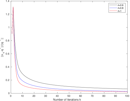
Figure 1. the effect of $\theta$ on the convergence of the algorithm (4.6)

References

- [1] H.H. Bauschke, P.L. Combettes, Convex analysis and monotone operator theory in Hilbert spaces, CMS Books in Mathematics, Springer, New York, (2011).
- [2] O. Guler, Foundations of optimization, Graduate Texts in Mathematics 258, SpringerScience+Bisiness Media, LLC 2010.
- [3] D.P. Bertsekas, Nonlinear programming, Athena Scientific, Belmont, Massachusetts, 1995.
- [4] H. Iiduka, W. Takahashi, Strong convergence theorems for nonexpansive mapping and inverse-strongly monotone mappings, Nonlinear Anal., 61 (2005), 341-350.
- [5] A. Moudafi, Viscosity approximation methods for fixed points problemes, J. Math. Anal. Appl. 241 (2000), 46-55.
- [6] J. Peypoquet, Convex optimization in normed spaces Theory, Methods, and Examples, Springer Briefs in Optimization.
- [7] W. Takahashi, M. Toyoda, Weak convergence theorems for noexpansive mappings and monotone mapping, J. Optim. Theory Appl., 118 (2003), 417-428.
- [8] H.K Xu, Iterative algorithms or nonlinear operators, J. Lond. Math. Soc. 65 (2002), 240-256.
- [9] H.K Xu, Avearged mapping and the gradient-projection algorithm, J. Optimi. Theory Appl. 150 (2011), 360-378.
- [10] Y.Y. Yao, YC. Liou, C.P. Chen, Algorithms construction for nonexpansive mapping and inverse-strongly monotone mapping, Taiwanese J. Math. 15 (5) (2011), 1979-1998.