HUPD-2210 Non-SUSY Lepton Flavor Model with 3HDM

1 Introduction

The standard model (SM) is the successful one with the discovery of the Higgs boson. In the particle physics, the gauge theory is applied and tested by the electroweak precision measurements for the SM. However there are still mysterious puzzles, e.g. the origin of the generations which are differences of the mixing angles and masses for quark and lepton sectors. Actually, the Yukawa couplings are completely free parameters so that the mixing angles and masses cannot be predicted in the SM. In addition, the neutrinos are massless for renormalizable operators. One of the attractive phenomena to solve the puzzles is the neutrino oscillation which provides us the useful informations such as three lepton mixing angles and two neutrino mass squared differences which mean that the neutrinos have non-zero masses. The T2K and NO$\nu$A experiments have confirmed the neutrino oscillation in the $\nu_{\mu}\to\nu_{e}$ appearance events [1, 2, 3], which are one of the clues of the new physics beyond the SM such as the Dirac CP violating phase for the lepton sector by combining the data of the reactor neutrino experiments [4, 5]. The KamLAND-Zen [6, 7], GERDA[8, 9], and CUORE [10, 11] experiments also provide us the significant informations which are whether the neutrinos are Dirac or Majorana particles, the lepton number violation, and Majorana phases if the neutrinos are Majorana particles. Thus the neutrino oscillation experiments go into a new phase of the precise determinations of the lepton mixing angles, the neutrino mass squared differences, and the CP violating phases.

The SM particles obey the gauge theory. After spontaneous symmetry breaking (SSB), the gauge bosons and fermions get the masses through the Higgs mechanism. However the Yukawa couplings cannot be controlled by the gauge symmetry, the Yukawa couplings are completely free parameters in the SM. The flavor symmetry can apply to the generations. The Froggatt-Nielsen mechanism which was proposed by C. D. Froggatt and H. B. Nielsen are introduced global $U(1)_{\text{FN}}$ symmetry [12]. Thanks for the $U(1)_{\text{FN}}$ symmetry, it is natural to explain the fermion mass hierarchies. On the other hand, the non-Abelian discrete symmetry (See for the review [13]-[17].) can naturally explain the lepton mixing angles so-called “tri-bimaximal mixing (TBM)” [18, 19] before the reactor experiments reported the non-zero reactor angle $\theta_{13}$ [4, 5]. Actually, many authors have studied the breaking or deviation from the TBM [20]-[42] or other patterns of the lepton mixing angles, e.g. tri-bimaximal-Cabibbo mixing [43, 44]. One of the successful flavor models was proposed by G. Altarelli and F. Feruglio [45, 46]. The Altarelli and Feruglio (AF) model show the TBM by using the non-Abelian discrete symmetry $A_{4}$. They introduced two SM gauge singlet scalar fields so-called “flavons” and taking the vacuum expectation value (VEV) alignments of the $A_{4}$ triplets as $(1,0,0)$ and $(1,1,1)$, which is naturally explained that the charged lepton is diagonal and neutrino mixing is TBM, respectively. However the corrected VEV alignments cannot be driven from the potential analysis. Then, they applied to the supersymmetry (SUSY) and introduced the “driving” fields. There are so many scalar fields in addition to the no evidence of the SUSY particles for the accelerator experiments, e.g. Large Hadron Collider experiment.

In this paper, we propose a simple non-SUSY lepton flavor model with $A_{4}$ symmetry. The $A_{4}$ group is a minimal one which includes triplet irreducible representation. We introduce three Higgs doublets which is assigned as triplet of the $A_{4}$ symmetry. It is natural that there are three generations as same as the SM fermions. We analyse the potential and we get the VEV for the local minimum in the three Higgs doublet model (3HDM) [47] with $A_{4}$ symmetry [48]-[61]. The left-handed lepton doublets are assigned to triplet and the right-handed charged leptons are assigned to different singlets of the $A_{4}$ symmetry, respectively. We introduce the right-handed Majorana neutrinos which are assigned to triplet of the $A_{4}$ symmetry. In our model, the right-handed Majorana neutrino mass matrix has a simple flavor structure. On the other hand, the Dirac neutrino mass matrix has symmetric and anti-symmetric Yukawa couplings for $A_{4}$ symmetry. By using the type-I seesaw mechanism [62, 63, 64, 65, 66], we obtain the left-handed Majorana neutrino mass matrix. After diagonalizing the charged lepton and left-handed Majorana neutrino mass matrices, we get the lepton mixing matrix which is Pontecorvo-Maki-Nakagawa-Sakata (PMNS) one [67, 68]. In the numerical analysis, we use the NuFIT 5.1 data [69, 70]. We find that only inverted ordering is acceptable and we cannot find the solutions for normal ordering in the neutrino mass hierarchy. We obtain relevant relations for mixing angles and the effective mass for the neutrino-less double beta ($0\nu\beta\beta$) decay as a function of the lightest neutrino mass. Especially, the Dirac CP phase and lepton mixing angle $\theta_{23}$ are strongly correlated. If the neutrinos are Majorana particles, the effective mass for the neutrino-less double beta decay and the lightest neutrino mass are also predicted in our model.

This paper is organized as follows. In Section 2, we briefly introduce the $A_{4}$ group. Next, we analyse the potential with $A_{4}$ symmetry. In Section 3, we present the $A_{4}$ flavor model and study mass matrices. In Section 4, we show the numerical analysis of our model. Section 5 is devoted to a summary and discussions. We show the relevant multiplication rule of the $A_{4}$ group in Appendix A.

2 Potential analysis in the 3HDM with $A_{4}$ symmetry

In this section, we discuss the 3HDM. First, we briefly introduce the $A_{4}$ group. Next, we analyse the potential with $A_{4}$ symmetry in the 3HDM, where we assign the three Higgs doublets as the triplet of the $A_{4}$ symmetry. It is natural that the Higgs fields are three generations as same as the SM fermions.

Let us analyse the potential in the 3HDM with $A_{4}$ symmetry. The $A_{4}$ group which is a minimal including triplet irreducible representation is the symmetric group of a tetrahedron or even permutation of four elements. There are twelve elements and four irreducible representations such as three different singlets $\bf{1}$, ${\bf 1^{\prime}}$, ${\bf 1^{\prime\prime}}$ and triplet ${\bf 3}$ in the $A_{4}$ group, respectively. Also the $A_{4}$ can be defined as the group generated by two elements $S$ and $T$ which satisfy the following algebraic relations as

$$S^{2}=T^{3}=(ST)^{3}={\bf 1}.$$ (1)

These generators are represented by

$${\bf 1}: \quad S=1,\quad T=1,$$

$${\bf 1^{\prime}}: \quad S=1,\quad T=e^{\frac{4\pi i}{3}}\equiv\omega^{2},$$ (2)

$${\bf 1^{\prime\prime}}: \quad S=1,\quad T=e^{\frac{2\pi i}{3}}\equiv\omega,$$

on the one-dimensional representations. These generators are also represented by

$${\bf 3}:\quad S=\frac{1}{3}\begin{pmatrix}-1&2&2\\ 2&-1&2\\ 2&2&-1\end{pmatrix},\quad T=\begin{pmatrix}1&0&0\\ 0&\omega^{2}&0\\ 0&0&\omega\end{pmatrix},$$ (3)

on the three-dimensional representation. In these bases Eqs. (2) and (3), we can make the character table and obtain the multiplication rules of the $A_{4}$ group. The relevant multiplication rule is shown in Appendix A.

We introduce three Higgs doublets $\phi_{1},\phi_{2},\phi_{3}$ which are assigned as triplet $\Phi$:

$$\Phi=(\phi_{1},\phi_{2},\phi_{3}),$$ (4)

of the $A_{4}$ symmetry. On the other hand, the complex conjugate of the $\Phi$ is considered by the conjugate of the generator $T$ of Eq. (3) as

$$T^{*}=\begin{pmatrix}1&0&0\\ 0&\omega&0\\ 0&0&\omega^{2}\end{pmatrix}.$$ (5)

Then, the complex conjugate of the $\Phi$ is given by

$$\Phi^{*}=(\phi_{1}^{*},\phi_{3}^{*},\phi_{2}^{*}),$$ (6)

and the multiplication rule of $A_{4}$ is kept as Eq. (A) in Appendix A. In our model, the Higgs potential is written as

$$V=-\mu^{2}\Phi^{{\dagger}}\Phi+\lambda(\Phi^{{\dagger}}\Phi)^{2}.$$ (7)

This potential is invariant for hte $SU(2)_{L}\times U(1)_{Y}$ of the SM and $A_{4}$ symmetry. By using the multiplication rule of $A_{4}$ in Appendix A, we obtain the Higgs potential as follows:

$$V= -\mu^{2}(|\phi_{1}|^{2}+|\phi_{2}|^{2}+|\phi_{3}|^{2})$$

$$+\lambda_{1}|\phi_{1}^{2}+2\phi_{2}\phi_{3}|^{2}+\lambda_{2}|\phi_{2}^{2}+2\phi_{3}\phi_{1}|^{2}+\lambda_{3}|\phi_{3}^{2}+2\phi_{1}\phi_{2}|^{2}$$

$$+\lambda_{4}\Big{[}|\phi_{1}^{2}-\phi_{2}\phi_{3}|^{2}+|\phi_{2}^{2}-\phi_{3}\phi_{1}|^{2}+|\phi_{3}^{2}-\phi_{1}\phi_{2}|^{2}\Big{]},$$ (8)

where we rewrite the coupling $4\lambda_{4}/9$ as $\lambda_{4}$ in our convention. We consider the potential minimum conditions as

$$\left(\frac{\partial V}{\partial\phi_{1}}\right)_{\phi_{1}=\langle\phi_{1}\rangle,\phi_{2}=\langle\phi_{2}\rangle,\phi_{3}=\langle\phi_{3}\rangle} =0,$$ (9)

$$\left(\frac{\partial V}{\partial\phi_{2}}\right)_{\phi_{1}=\langle\phi_{1}\rangle,\phi_{2}=\langle\phi_{2}\rangle,\phi_{3}=\langle\phi_{3}\rangle} =0,$$ (10)

$$\left(\frac{\partial V}{\partial\phi_{3}}\right)_{\phi_{1}=\langle\phi_{1}\rangle,\phi_{2}=\langle\phi_{2}\rangle,\phi_{3}=\langle\phi_{3}\rangle} =0.$$ (11)

From Eqs. (2)-(11) we obtain the following conditions:

$$0= -2\mu^{2}v_{1}+4\lambda_{1}v_{1}(v_{1}^{2}+2v_{2}v_{3})+4\lambda_{2}v_{3}(v_{2}^{2}+2v_{3}v_{1})+4\lambda_{3}v_{2}(v_{3}^{2}+2v_{1}v_{2})$$

$$+4\lambda_{4}\Big{[}v_{1}(v_{1}^{2}-v_{2}v_{3})-\frac{1}{2}v_{2}(v_{3}^{2}-v_{1}v_{2})-\frac{1}{2}v_{3}(v_{2}^{2}-v_{3}v_{1})\Big{]},$$ (12)

$$0= -2\mu^{2}v_{2}+4\lambda_{1}v_{3}(v_{1}^{2}+2v_{2}v_{3})+4\lambda_{2}v_{2}(v_{2}^{2}+2v_{3}v_{1})+4\lambda_{3}v_{1}(v_{3}^{2}+2v_{1}v_{2})$$

$$+4\lambda_{4}\Big{[}v_{2}(v_{2}^{2}-v_{3}v_{1})-\frac{1}{2}v_{1}(v_{3}^{2}-v_{1}v_{2})-\frac{1}{2}v_{3}(v_{1}^{2}-v_{2}v_{3})\Big{]},$$ (13)

$$0= -2\mu^{2}v_{3}+4\lambda_{1}v_{2}(v_{1}^{2}+2v_{2}v_{3})+4\lambda_{2}v_{1}(v_{2}^{2}+2v_{3}v_{1})+4\lambda_{3}v_{3}(v_{3}^{2}+2v_{1}v_{2})$$

$$+4\lambda_{4}\Big{[}v_{3}(v_{3}^{2}-v_{1}v_{2})-\frac{1}{2}v_{1}(v_{2}^{2}-v_{3}v_{1})-\frac{1}{2}v_{2}(v_{1}^{2}-v_{2}v_{3})\Big{]}.$$ (14)

We sum the conditions Eqs. (12)-(14) and we obtain a equation as follows:

$$0= (v_{1}+v_{2}+v_{3})\Big{[}-2\mu^{2}+4\lambda_{1}(v_{1}^{2}+2v_{1}v_{2})+4\lambda_{2}(v_{2}^{2}+2v_{3}v_{1})+4\lambda_{3}(v_{3}^{2}+2v_{1}v_{2})$$

$$+4\lambda_{4}(v_{1}^{2}+v_{2}^{2}+v_{3}^{2}-v_{1}v_{2}-v_{2}v_{3}-v_{3}v_{1})\Big{]}$$

$$= 4(v_{1}+v_{2}+v_{3})\Big{[}(\lambda_{1}+\lambda_{4})v_{1}^{2}+\big{\{}(2\lambda_{3}-\lambda_{4})v_{2}+(2\lambda_{2}-\lambda_{4})v_{3}\big{\}}v_{1}$$

$$+(\lambda_{2}+\lambda_{4})v_{2}^{2}+(\lambda_{3}+\lambda_{4})v_{3}^{2}+(2\lambda_{1}-\lambda_{4})v_{2}v_{3}-\frac{\mu^{2}}{2}\Big{]}.$$ (15)

When $v_{1}+v_{2}+v_{3}\neq 0$ is satisfied, we obtain

$$(\lambda_{1}+\lambda_{4})v_{1}^{2}+\big{\{}(2\lambda_{3}-\lambda_{4})v_{2}+(2\lambda_{2}-\lambda_{4})v_{3}\big{\}}v_{1}$$

$$+(\lambda_{2}+\lambda_{4})v_{2}^{2}+(\lambda_{3}+\lambda_{4})v_{3}^{2}+(2\lambda_{1}-\lambda_{4})v_{2}v_{3}-\frac{\mu^{2}}{2}=0.$$ (16)

If $\lambda_{1}+\lambda_{4}$ which is the coefficient of $v_{1}^{2}$ in Eq. (2) holds zero, we find the solution $(1,1,1)$. In this case we cannot realize the current experimental data. When $\lambda_{1}+\lambda_{4}\neq 0$, $\lambda_{3}=\lambda_{2}$, and $2\lambda_{1}+2\lambda_{2}+\lambda_{4}\neq 0$ hold, we obtain the following solutions:

$$\langle\phi_{1}\rangle= v_{1},$$ (17)

$$\langle\phi_{2}\rangle= v_{2}$$ (18)

$$= -\frac{2\lambda_{2}-\lambda_{4}}{2\lambda_{1}+2\lambda_{2}+\lambda_{4}}v_{1}$$

$$\pm\frac{\sqrt{\{-2\lambda_{1}^{2}+2\lambda_{2}^{2}-2\lambda_{2}(\lambda_{1}-3\lambda_{4})-3\lambda_{1}\lambda_{4}\}v_{1}^{2}+\frac{1}{2}\left(2\lambda_{1}+2\lambda_{2}+\lambda_{4}\right)\mu^{2}}}{2\lambda_{1}+2\lambda_{2}+\lambda_{4}},$$

$$\langle\phi_{3}\rangle= v_{3}$$ (19)

$$= -\frac{2\lambda_{2}-\lambda_{4}}{2\lambda_{1}+2\lambda_{2}+\lambda_{4}}v_{1}$$

$$\pm\frac{\sqrt{\{-2\lambda_{1}^{2}+2\lambda_{2}^{2}-2\lambda_{2}(\lambda_{1}-3\lambda_{4})-3\lambda_{1}\lambda_{4}\}v_{1}^{2}+\frac{1}{2}\left(2\lambda_{1}+2\lambda_{2}+\lambda_{4}\right)\mu^{2}}}{2\lambda_{1}+2\lambda_{2}+\lambda_{4}}.$$

These VEVs can be written as

$$v_{1}=v\cos{\beta},\quad v_{2}=\frac{v}{\sqrt{2}}\sin{\beta},\quad v_{3}=\frac{v}{\sqrt{2}}\sin{\beta},$$ (20)

where, the range of $\lambda$ are $\lambda_{1}<\lambda_{2}$ and $\lambda_{1}<\lambda_{4}$. These $\lambda$ conditions are derived from minimum conditions of Higgs potential.

Note that there are other two solution forms in Eq. (20). When $\lambda_{3}=\lambda_{1}$, $\lambda_{2}+\lambda_{4}\neq 0$ and $2\lambda_{1}+2\lambda_{2}+\lambda_{4}\neq 0$ hold, we obtain

$$v_{1}=\frac{v}{\sqrt{2}}\sin{\beta},\quad v_{2}=v\cos{\beta},\quad v_{3}=\frac{v}{\sqrt{2}}\sin{\beta}.$$ (21)

On the other hand, when $\lambda_{2}=\lambda_{1}$, $\lambda_{3}+\lambda_{4}\neq 0$ and $2\lambda_{1}+2\lambda_{3}+\lambda_{4}\neq 0$ hold, we obtain

$$v_{1}=\frac{v}{\sqrt{2}}\sin{\beta},\quad v_{2}=\frac{v}{\sqrt{2}}\sin{\beta},\quad v_{3}=v\cos{\beta}.$$ (22)

In the next section, we present our $A_{4}$ model and caluculate the mass matries.

3 Lepton flavor model in the $A_{4}$ symmetry

In this section, we present a non-SUSY lepton flavor model in the $A_{4}$ symmetry. The left-handed lepton doublets are assigned to triplet and the right-handed charged leptons are assigned to different singlets as ${\bf 1}$, ${\bf 1^{\prime\prime}}$, and ${\bf 1^{\prime}}$ of the $A_{4}$ symmetry, respectively. We introduce the right-handed Majorana neutrinos which are assigned to triplet of the $A_{4}$ symmetry. We also introduce three Higgs doublets which are assigned as triplet of the $A_{4}$ symmetry as discussed in Section 2. In Table 1, we summarize the particle assignments of $SU(2)_{L}$ and $A_{4}$ symmetry.

	$\bar{\ell}=(\bar{\ell}_{e},\bar{\ell}_{\mu},\bar{\ell}_{\tau})$	$e_{R}$	$\mu_{R}$	$\tau_{R}$	$\nu_{R}=(\nu_{R1},\nu_{R2},\nu_{R3})$	$\Phi=(\phi_{1},\phi_{2},\phi_{3})$
$SU(2)_{L}$	$2$	$1$	$1$	$1$	$1$	2
$A_{4}$	${\bf 3}$	${\bf 1}$	${\bf 1^{\prime\prime}}$	${\bf 1^{\prime}}$	${\bf 3}$	${\bf 3}$

Table 1: The charge assignments of $SU(2)_{L}\times A_{4}$ symmetry in our model.

We can write down the Lagrangian for Yukawa interactions and Majorana mass term in our model. The $SU(2)_{L}\times A_{4}$ invariant Lagrangian is written as

$$\mathcal{L}_{Y}=\mathcal{L}_{\ell}+\mathcal{L}_{D}+\mathcal{L}_{M}+h.c.,$$ (23)

where

$$\mathcal{L}_{\ell} =y_{e}\bar{\ell}\Phi e_{R}+y_{\mu}\bar{\ell}\Phi\mu_{R}+y_{\tau}\bar{\ell}\Phi\tau_{R},$$ (24)

$$\mathcal{L}_{D} =y_{D}\bar{\ell}\tilde{\Phi}\nu_{R},$$ (25)

$$\mathcal{L}_{M} =\frac{1}{2}M\bar{\nu}_{R}^{c}\nu_{R}.$$ (26)

Note that $y_{e},y_{\mu},y_{\tau}$, and $y_{D}$ are Yukawa couplings and $M$ is the right-handed Majorana neutrino mass. After the SSB, three Higgs doublets have VEVs as $\braket{\Phi}=(v_{1},v_{2},v_{3})$. In the charged lepton sector Eq. (24), the Yukawa interactions are rewritten as

$$y_{e}\bar{\ell}\Phi e_{R} =y_{e}(\bar{\ell}_{e}\phi_{1}+\bar{\ell}_{\mu}\phi_{3}+\bar{l}_{\tau}\phi_{2})e_{R}$$ (27)

$$=y_{e}(\bar{e}_{L}v_{1}+\bar{\mu}_{L}v_{3}+\bar{\tau}_{L}v_{2})e_{R},$$

$$y_{\mu}\bar{\ell}\Phi\mu_{R} =y_{\mu}(\bar{\ell}_{\tau}\phi_{3}+\bar{\ell}_{e}\phi_{2}+\bar{\ell}_{\mu}\phi_{1})\mu_{R}$$ (28)

$$=y_{\mu}(\bar{\tau}_{L}v_{3}+\bar{e}_{L}v_{2}+\bar{\mu}_{L}v_{1})\mu_{R},$$

$$y_{\tau}\bar{\ell}\Phi\tau_{R} =y_{\tau}(\bar{\ell}_{\mu}\phi_{2}+\bar{\ell}_{e}\phi_{3}+\bar{\ell}_{\tau}\phi_{1})\tau_{R}$$ (29)

$$=y_{\tau}(\bar{\mu}_{L}v_{2}+\bar{e}_{L}v_{3}+\bar{\tau}_{L}v_{1})\tau_{R}.$$

Then, the charged lepton mass matrix $M_{\ell}$ is obtained as

$$M_{\ell}=\begin{pmatrix}y_{e}v_{1}&y_{\mu}v_{2}&y_{\tau}v_{3}\\ y_{e}v_{3}&y_{\mu}v_{1}&y_{\tau}v_{2}\\ y_{e}v_{2}&y_{\mu}v_{3}&y_{\tau}v_{1}\\ \end{pmatrix}_{LR}.$$ (30)

Here and hereafter we take the left-right basis in the mass matrices. In order to obtain the left-side unitary mixing matrix $U_{\ell}$, we consider $M_{\ell}M_{\ell}^{\dagger}$ as

$$M_{\ell}M_{\ell}^{\dagger}=$$ (31)

$$\begin{pmatrix}|y_{e}|^{2}v_{1}^{2}+|y_{\mu}|^{2}v_{2}^{2}+|y_{\tau}|^{2}v_{3}^{2}&|y_{e}|^{2}v_{1}v_{3}+|y_{\mu}|^{2}v_{1}v_{2}+|y_{\tau}|^{2}v_{2}v_{3}&|y_{e}|^{2}v_{1}v_{2}+|y_{\mu}|^{2}v_{2}v_{3}+|y_{\tau}|^{2}v_{1}v_{3}\\ \dots&|y_{e}|^{2}v_{3}^{2}+|y_{\mu}|^{2}v_{1}^{2}+|y_{\tau}|^{2}v_{2}^{2}&|y_{e}|^{2}v_{2}v_{3}+|y_{\mu}|^{2}v_{1}v_{3}+|y_{\tau}|^{2}v_{1}v_{2}\\ \dots&\dots&|y_{e}|^{2}v_{2}^{2}+|y_{\mu}|^{2}v_{3}^{2}+|y_{\tau}|^{2}v_{1}^{2}\end{pmatrix}.$$

Then, the elements of the mass matrix Eq. (31) are real and we can numerically calculate the charged lepton masses in Section 4. Next, we derive the Dirac neutrino mass matrix from Eq. (25). By using the $A_{4}$ multiplication rule (See appendix A.), we can make the singlet term. When we take the complex conjugate, we need to take care $\tilde{\Phi}=(\tilde{\phi}_{1},\tilde{\phi}_{3},\tilde{\phi}_{2})$ because of the complex conjugate for the generator $T$ in Eq. (5). Since Eq. (25) is $3\otimes 3\otimes 3$ form in $A_{4}$ symmetry, we first make $3_{S}\oplus 3_{A}\in 3\otimes 3$ as

$$y_{D}\bar{\ell}\tilde{\Phi}=\frac{y_{DS}}{3}\begin{pmatrix}2\bar{\ell}_{e}\tilde{\phi}_{1}-\bar{\ell}_{\mu}\tilde{\phi}_{2}-\bar{\ell}_{\tau}\tilde{\phi}_{3}\\ 2\bar{\ell}_{\tau}\tilde{\phi}_{2}-\bar{\ell}_{e}\tilde{\phi}_{3}-\bar{\ell}_{\mu}\tilde{\phi}_{1}\\ 2\bar{\ell}_{\mu}\tilde{\phi}_{3}-\bar{\ell}_{\tau}\tilde{\phi}_{1}-\bar{\ell}_{e}\tilde{\phi}_{2}\end{pmatrix}_{3_{S}}+\frac{y_{DA}}{2}\begin{pmatrix}\bar{\ell}_{\mu}\tilde{\phi}_{2}-\bar{\ell}_{\tau}\tilde{\phi}_{3}\\ \bar{\ell}_{e}\tilde{\phi}_{3}-\bar{\ell}_{\mu}\tilde{\phi}_{1}\\ \bar{\ell}_{\tau}\tilde{\phi}_{1}-\bar{\ell}_{e}\tilde{\phi}_{2}\\ \end{pmatrix}_{3_{A}},$$ (32)

where $y_{DS}$ and $y_{DA}$ are the symmetric and anti-symmetric Dirac Yukawa couplings, respectively. Then, the Dirac neutrino Yukawa interaction in Eq. (25) can be written as follows:

$$y_{D}\bar{\ell}\tilde{\Phi}\nu_{R}= \frac{y_{DS}}{3}\begin{pmatrix}2\bar{\ell}_{e}\tilde{\phi}_{1}-\bar{\ell}_{\mu}\tilde{\phi}_{2}-\bar{\ell}_{\tau}\tilde{\phi}_{3}\\ 2\bar{\ell}_{\tau}\tilde{\phi}_{2}-\bar{\ell}_{e}\tilde{\phi}_{3}-\bar{\ell}_{\mu}\tilde{\phi}_{1}\\ 2\bar{\ell}_{\mu}\tilde{\phi}_{3}-\bar{\ell}_{\tau}\tilde{\phi}_{1}-\bar{\ell}_{e}\tilde{\phi}_{2}\end{pmatrix}_{3_{S}}\otimes\begin{pmatrix}\nu_{R1}\\ \nu_{R2}\\ \nu_{R3}\end{pmatrix}+\frac{y_{DA}}{2}\begin{pmatrix}\bar{\ell}_{\mu}\tilde{\phi}_{2}-\bar{\ell}_{\tau}\tilde{\phi}_{3}\\ \bar{\ell}_{e}\tilde{\phi}_{3}-\bar{\ell}_{\mu}\tilde{\phi}_{1}\\ \bar{\ell}_{\tau}\tilde{\phi}_{1}-\bar{\ell}_{e}\tilde{\phi}_{2}\\ \end{pmatrix}_{3_{A}}\otimes\begin{pmatrix}\nu_{R1}\\ \nu_{R2}\\ \nu_{R3}\end{pmatrix}$$ (33)

$$= \frac{y_{DS}}{3}\left[(2\bar{\ell}_{e}\tilde{\phi}_{1}-\bar{\ell}_{\mu}\tilde{\phi}_{2}-\bar{\ell}_{\tau}\tilde{\phi}_{3})\nu_{R1}+(2\bar{\ell}_{\tau}\tilde{\phi}_{2}-\bar{\ell}_{e}\tilde{\phi}_{3}-\bar{\ell}_{\mu}\tilde{\phi}_{1})\nu_{R3}\right.$$ (34)

$$\qquad\qquad+\left.(2\bar{\ell}_{\mu}\tilde{\phi}_{3}-\bar{\ell}_{\tau}\tilde{\phi}_{1}-\bar{\ell}_{e}\tilde{\phi}_{2})\nu_{R2}\right]$$

$$+\frac{y_{DA}}{2}\left[(\bar{\ell}_{\mu}\tilde{\phi}_{2}-\bar{\ell}_{\tau}\tilde{\phi}_{3})\nu_{R1}+(\bar{\ell}_{e}\tilde{\phi}_{3}-\bar{\ell}_{\mu}\tilde{\phi}_{1})\nu_{R3}+(\bar{\ell}_{\tau}\tilde{\phi}_{1}-\bar{\ell}_{e}\tilde{\phi}_{2})\nu_{R2}\right],$$

where $\tilde{\Phi}=-i\sigma_{2}\Phi^{*}$ and the VEVs of $\tilde{\phi}_{i}$ are $\braket{\tilde{\phi_{i}}}=v_{i}$. Therefore, the Dirac neutrino mass matrix $M_{D}$ is obtained as

$$M_{D}=\frac{y_{DS}}{3}\begin{pmatrix}2v_{1}&-v_{2}&-v_{3}\\ -v_{2}&2v_{3}&-v_{1}\\ -v_{3}&-v_{1}&2v_{2}\end{pmatrix}_{LR}+\frac{y_{DA}}{2}\begin{pmatrix}0&-v_{2}&v_{3}\\ v_{2}&0&-v_{1}\\ -v_{3}&v_{1}&0\end{pmatrix}_{LR}.$$ (35)

Next we discuss the right-handed Majorana neutrino mass matrix. In Eq. (26), the right-handed Majorana neutrino mass term is decomposed as follows:

$$M\bar{\nu}_{R}^{c}\nu_{R}=M(\bar{\nu}_{R1}^{c}\nu_{R1}+\bar{\nu}_{R2}^{c}\nu_{R3}+\bar{\nu}_{R3}^{c}\nu_{R2}).$$ (36)

Then, the right-handed Majorana neutrino mass matrix $M_{R}$ is

$$M_{R}=M\begin{pmatrix}1&0&0\\ 0&0&1\\ 0&1&0\end{pmatrix}.$$ (37)

By using the type-I seesaw mechanism [62, 63, 64, 65, 66], the left-handed Majorana neutrino mass matrix $m_{\nu}$ is written as

$$m_{\nu}=-M_{D}M_{R}^{-1}M_{D}^{T}$$ (38)

$$= \frac{1}{M}\begin{pmatrix}2v_{2}v_{3}(y_{DA}^{2}-y_{DS}^{2})&v_{1}v_{2}(y_{DS}^{2}-4y_{DS}y_{DA}-y_{DA}^{2})&v_{1}v_{3}(y_{DS}^{2}+4y_{DS}y_{DA}-y_{DA}^{2})\\ v_{1}v_{2}(y_{DS}^{2}-4y_{DS}y_{DA}-y_{DA}^{2})&4v_{1}v_{3}y_{DS}(y_{DS}+y_{DA})&-y_{DS}^{2}(v_{1}^{2}+5v_{2}v_{3})\\ v_{1}v_{3}(y_{DS}^{2}+4y_{DS}y_{DA}-y_{DA}^{2})&-y_{DS}^{2}(v_{1}^{2}+5v_{2}v_{3})&4v_{1}v_{2}y_{DS}(y_{DS}-y_{DA})\end{pmatrix}$$

$$\quad+\frac{1}{M}\begin{pmatrix}-4v_{1}^{2}y_{DS}^{2}&2v_{3}^{2}y_{DS}(y_{DS}-y_{DA})&2v_{2}^{2}y_{DS}(y_{DS}+y_{DA})\\ 2v_{3}^{2}y_{DS}(y_{DS}-y_{DA})&-v_{2}^{2}(y_{DA}-y_{DS})^{2}&y_{DA}^{2}(v_{1}^{2}+v_{2}v_{3})\\ 2v_{2}^{2}y_{DS}(y_{DS}+y_{DA})&y_{DA}^{2}(v_{1}^{2}+v_{2}v_{3})&-v_{3}^{2}(y_{DA}-y_{DS})^{2}\end{pmatrix},$$

where we redefine the Dirac Yukawa couplings $y_{DS}/3\to y_{DS}$ and $y_{DA}/2\to y_{DA}$ for simplicity. In our model, the Dirac neutrino mass matrix has symmetric and anti-symmetric Yukawa couplings for the $A_{4}$ symmetry in Eq. (35). On the other hand, in Eq. (37), the right-handed Majorana neutrino mass matrix has a simple flavor structure, c.f., in the AF Model the Dirac neutrino mass matrix is simple. On the other hand, the right-handed Majorana neutrino mass matrix is the structure which derives the TBM in their model. In the next section, we show the numerical analysis.

4 Numerical analysis

In this section, we show the numerical analysis such as the lepton flavor mixing angles, Dirac CP phase, Majorana phases, and the effective mass for the $0\nu\beta\beta$ decay. We discuss what is our model verifiable in the near future experiments.

In section 2, we have analyzed the Higgs potential and found the following solution which was derived from Higgs potential minimization as

$$(v_{1},v_{2},v_{3})=(v\cos\beta,\frac{v}{\sqrt{2}}\sin\beta,\frac{v}{\sqrt{2}}\sin\beta).$$ (39)

Since charged lepton mass matrix Eq. (31) is only depend on three Yukawa couplings and Higgs VEVs. Then once we fix the Higgs VEVs, we can obtain charged lepton Yukawa couplings by solving the following equations and the unitary matrix which diagonalizes charged lepton mass matrix.

$$\mathrm{Tr}(M_{\ell}M_{\ell}^{\dagger}) =m_{e}^{2}+m_{\mu}^{2}+m_{\tau}^{2},$$

$$\mathrm{Det}(M_{\ell}M_{\ell}^{\dagger}) =m_{e}^{2}m_{\mu}^{2}m_{\tau}^{2},$$ (40)

$$\left(\mathrm{Tr}M_{\ell}M_{\ell}^{\dagger}\right)^{2}-\mathrm{Tr}\left[(M_{\ell}M_{\ell}^{\dagger})^{2}\right] =2(m_{e}^{2}m_{\mu}^{2}+m_{\mu}^{2}m_{\tau}^{2}+m_{\tau}^{2}m_{e}^{2}),$$

where $m_{e},m_{\mu},m_{\tau}$ are charged lepton masses. The Dirac neutrino Yukawa couplings similarly obtained by solving equations which are substituted Eq. (38) into Eq. (4), where we use the left-handed Majorana neutrino masses instead of the charged lepton masses in the right-side of Eq. (4). However neutrino masses are only known mass squared differences $\Delta m_{21}^{2}$ and $\Delta m_{32(31)}^{2}$ in the inverted (normal) ordering of the neutrino mass hierarchy. Then we need to decide the Dirac neutrino Yukawa couplings $y_{DS}$ and $y_{DA}$ to satisfy experimental data in Table 2.

Inverted Ordering	bfp $\pm 1\sigma$	$3\sigma$ range
$\sin^{2}\theta_{12}$	$0.304^{+0.013}_{-0.012}$	$0.269\to 0.343$
$\theta_{12}/^{\circ}$	$33.45^{+0.78}_{-0.75}$	$31.27\to 35.87$
$\sin^{2}\theta_{23}$	$0.570^{+0.016}_{-0.022}$	$0.410\to 0.613$
$\theta_{23}/^{\circ}$	$49.0^{+0.9}_{-1.3}$	$39.8\to 51.6$
$\sin^{2}\theta_{13}$	$0.02241^{+0.00074}_{-0.00062}$	$0.02055\to 0.02457$
$\theta_{13}/^{\circ}$	$8.61^{+0.14}_{-0.12}$	$8.24\to 9.02$
$\delta_{\mathrm{CP}}/^{\circ}$	$278^{+22}_{-30}$	$194\to 345$
$\frac{\Delta m_{21}^{2}}{10^{-5}[\mathrm{eV}^{2}]}$	$7.42^{+0.21}_{-0.20}$	$6.82\to 8.04$
$\frac{\Delta m_{32}^{2}}{10^{-3}[\mathrm{eV}^{2}]}$	$-2.490^{+0.026}_{-0.028}$	$-2.574\to-2.410$

Table 2: NuFIT 5.1 data [69, 70] in the inverted neutirno mass ordering, where $\Delta m^{2}_{ij}$ is mass squared difference between $m_{i}$ and $m_{j}$.

In our numerical analysis, we simulate by assigning different numerical values to the lightest neutrino mass at the range $m_{3}\in[0,15.9]$ [meV], where the upper limit of the lightest neutrino mass is estimated in Ref. [71]. We analyze our model in normal and inverted neutrino mass orderings. When we assume the normal ordering, there are no realistic parameters which satisfy the current experimental data in Table 2. We then assume the inverted ordering for the rest of our discussion. In Fig. 1, we show the symmetric and anti-symmetric Dirac Yukawa couplings for Eq. (35) which are satisfied the current experimental data in Table 2. These Yukawa couplings look like proportional each other and $\mathcal{O}(1)$. The Majorana mass $M$ in Eq. (37) is allowed at $\mathcal{O}(10^{15})$ [GeV]. We also show the numerical results of the Higgs VEV ratio $\tan\beta$ and the complex phase of the Dirac Yukawa coupling in Fig. 1. The $\tan\beta$ is localized around $\tan\beta\in[0.4,0.6],[0.8,1.2]$. The complex phase of the Dirac Yukawa coupling $\phi_{DA}$ only appear in $70[{\ }^{\circ}]$ - $100[{\ }^{\circ}]$. In our model, the complex phase of the Dirac Yukawa coupling which contribute to the mixing matrix is only $\phi_{DA}$, then this result has a strong influence to the CP phases.

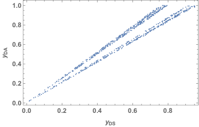
(a)

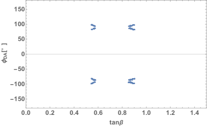
(b)

Figure 1: (a) The relation between the Dirac neutrino Yukawa couplings $y_{DS}$ and $y_{DA}$. We simulate by assigning different numerical values to the Dirac neutrino Yukawa couplings at $\mathcal{O}(1)$. (b) Higgs VEV ratio $\tan\beta$ and complex phase of the Dirac Yukawa coupling $\phi_{DA}$.

In the PDG parametrization, we can write the PMNS matrix as

$$\qquad\qquad U_{\mathrm{PMNS}}^{\text{PDG}}=\begin{pmatrix}U_{e1}&U_{e2}&U_{e3}\\ U_{\mu 1}&U_{\mu 2}&U_{\mu 3}\\ U_{\tau 1}&U_{\tau 2}&U_{\tau 3}\end{pmatrix}$$ (41)

$$=\begin{pmatrix}c_{12}c_{13}&s_{12}c_{13}&s_{13}\mathrm{e}^{-i\delta_{\mathrm{CP}}}\\ -s_{12}c_{23}-c_{12}s_{23}s_{13}\mathrm{e}^{i\delta_{\mathrm{CP}}}&c_{12}c_{23}-s_{12}s_{23}s_{13}\mathrm{e}^{i\delta_{\mathrm{CP}}}&s_{23}c_{13}\\ s_{12}s_{23}-c_{12}c_{23}s_{13}\mathrm{e}^{i\delta_{\mathrm{CP}}}&-c_{12}s_{23}-s_{12}c_{23}s_{13}\mathrm{e}^{i\delta_{\mathrm{CP}}}&c_{23}c_{13}\end{pmatrix}\begin{pmatrix}\mathrm{e}^{i\eta_{1}}&&\\ &\mathrm{e}^{i\eta_{2}}&\\ &&1\\ \end{pmatrix},$$

where $U_{\alpha i}~{}(\alpha=e,\mu,\tau,~{}i=1,2,3)$ are the PMNS matrix elements, $c_{ij}$ and $s_{ij}$ denote $\cos\theta_{ij}$ and $\sin\theta_{ij}$, $\delta_{\text{CP}}$ is the Dirac CP phase, and $\eta_{1}$ and $\eta_{2}$ are Majorana phases, respectively [72]. The lepton mixing angles are obtained as follows:

$$\sin\theta_{13}=\left|U_{e3}\right|,\quad\tan\theta_{12}=\left|\frac{U_{e2}}{U_{e1}}\right|,\quad\tan\theta_{23}=\left|\frac{U_{\mu 3}}{U_{\tau 3}}\right|.$$ (42)

In addition, the Dirac CP phase is determined by one of the Jarlskog Invariants [73] as

$$J_{\text{CP}}=\text{Im}\left[U_{e1}U_{e2}^{*}U_{\mu 2}U_{\mu 1}^{*}\right],$$ (43)

and

$$J_{\text{CP}}=\sin\theta_{12}\cos\theta_{12}\sin\theta_{23}\cos\theta_{23}\sin\theta_{13}\cos^{2}\theta_{13}\sin\delta_{\text{CP}},$$ (44)

in the PDG parametrization in Ref. [72]. The $\delta_{\text{CP}}$ is also determined by one of the absolute values for PMNS mixing matrix elements:

$$\left|U_{\tau 1}\right|^{2}= \sin^{2}\theta_{12}\sin^{2}\theta_{23}+\cos^{2}\theta_{12}\cos^{2}\theta_{23}\sin^{2}\theta_{13}$$

$$-2\sin\theta_{12}\sin\theta_{23}\cos\theta_{12}\cos\theta_{23}\sin\theta_{13}\cos\delta_{\text{CP}}.$$ (45)

Then, we can determine the $\delta_{\text{CP}}$. In Fig. 2, we show the allowed region for the $\sin^{2}\theta_{23}$ and $\delta_{\text{CP}}$ within $3\sigma$ standard deviation of the Table 2. The gray area is outside of $3\sigma$ standard deviation of $\delta_{\text{CP}}$ for NuFIT 5.1 data in Ref. [69, 70]. The relation between $\sin^{2}\theta_{23}$ and Dirac CP phase $\delta_{\text{CP}}$ has strong correlation. Especially, in $\sin^{2}\theta_{23}\in[0.41,0.52]$, this relation has one to one correspondence because the complex phase comes from one Yukawa coupling phase $\phi_{DA}$. Then if the $\theta_{23}$ is more precise measured by the future neutrino oscillation experiments, the Dirac CP phase is more precise predicted, and vice versa.

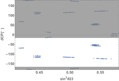
Figure 2: The allowed region for the $\sin^{2}\theta_{23}$ and $\delta_{\text{CP}}$ within $3\sigma$ standard deviation of the Table 2. The gray area is outside of $3\sigma$ standard deviation in NuFIT 5.1 data [69, 70].

We can diagonalize the $m_{\nu}m_{\nu}^{\dagger}$ in Eq. (38) by using the unitary matrix $U_{\nu}$. We can also diagonalize the complex symmetric matrix $m_{\nu}$ by using $U_{\nu}$ as follows:

$$U_{\nu}^{\dagger}m_{\nu}U_{\nu}^{*}=\mathrm{diag}(m_{1}\mathrm{e}^{i\zeta_{1}},m_{2}\mathrm{e}^{i\zeta_{2}},m_{3}\mathrm{e}^{i\zeta_{3}}).$$ (46)

In order to remove these phases from mass diagonal matrix, we need to multiply phase diagonal matrix $P_{\nu}=\mathrm{diag}(\mathrm{e}^{i\zeta_{1}/2},\mathrm{e}^{i\zeta_{2}/2},\mathrm{e}^{i\zeta_{3}/2})$ on both sides of Eq (46),

$${P_{\nu}}^{\dagger}({U_{\nu}}^{\dagger}m_{\nu}{U_{\nu}}^{*}){P_{\nu}}^{*}=\mathrm{diag}(m_{1},m_{2},m_{3}).$$ (47)

Then, the unitary matrix $U_{\nu}P_{\nu}$ makes the mass matrix real diagonal. Similarly, we diagonalize $M_{\ell}M_{\ell}^{\dagger}$ in Eq (31) by using the unitary matrix $U_{\ell}$. Therefore we can calculate the PMNS matrix in our model as follows:

$$U_{\text{PMNS}}^{\text{mod}}= {U_{\ell}}^{\dagger}U_{\nu}P_{\nu}$$

$$= \begin{pmatrix}U_{e1}^{\text{mod}}&U_{e2}^{\text{mod}}&U_{e3}^{\text{mod}}\\ U_{\mu 1}^{\text{mod}}&U_{\mu 2}^{\text{mod}}&U_{\mu 3}^{\text{mod}}\\ U_{\tau 1}^{\text{mod}}&U_{\tau 2}^{\text{mod}}&U_{\tau 3}^{\text{mod}}\end{pmatrix}.$$ (48)

The Majorana phases $\eta_{1}$ and $\eta_{2}$ are determined by using PMNS matrix in Eq. (4) as follows:

$$\eta_{1}=\text{arg}\left[\frac{U_{e1}^{\text{mod}}U_{e3}^{\text{mod}*}}{\cos\theta_{12}\cos\theta_{13}\sin\theta_{13}e^{i\delta_{\text{CP}}}}\right],\quad\eta_{2}=\text{arg}\left[\frac{U_{e2}^{\text{mod}}U_{e3}^{\text{mod}*}}{\sin\theta_{12}\cos\theta_{13}\sin\theta_{13}e^{i\delta_{\text{CP}}}}\right].$$ (49)

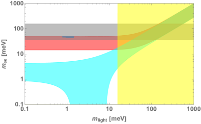
(a)

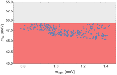
(b)

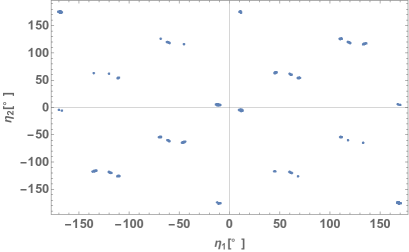
(c)

Figure 3: (a) The relation between the effective mass for $0\nu\beta\beta$ decay $m_{ee}$ and lightest neutrino mass. The red area and blue area are model independent analyses for the inverted ordering and normal ordering of the neutrino mass hierarchies, respectively. The gray area is upper limit on the effective mass of 36 - 156 [meV] at $90\%$ C.L. in Ref. [7]. The yellow area is upper limit on the lightest neutrino mass $m_{3}\simeq 15.9$ [meV] which is estimated in Ref. [71]. (b) The enlargement of figure (a). (c) The relation between Majorana phases $\eta_{1}$ and $\eta_{2}$.

The 0$\nu\beta\beta$ decay is determined by the magnitude of the lightest neutrino mass and neutrino mass ordering. In Figs. 3 and 3 , we show the prediction of the effective mass $m_{ee}$ for the $0\nu\beta\beta$ decay as

$$m_{ee}=\left|\sum_{i=1}^{3}m_{i}{U_{ei}^{\text{mod}}}^{2}\right|=\left|m_{1}{U_{e1}^{\text{mod}}}^{2}+m_{2}{U_{e2}^{\text{mod}}}^{2}+m_{3}{U_{e3}^{\text{mod}}}^{2}\right|.$$ (50)

Note that only inverted ordering is acceptable then the lightest neutrino mass is $m_{3}$. The lightest neutrino mass $m_{3}$ appears in $0.789$ - $1.43~{}[\mathrm{meV}]$ which is the within the Planck data [71] and the effective mass takes very restricted region $m_{ee}\simeq 47.1~{}[\mathrm{meV}]$. This value is in upper limit on the effective mass of 36 - 156 [meV] at $90\%$ C.L. in Ref. [7]. Then this model can be verified in the near future neutrino experiments, e.g. the KamLAND-Zen [6, 7], GERDA[8, 9], and CUORE [10, 11] experiments. In Fig. 3, we show the relation among Majorana phases $\eta_{1}$ and $\eta_{2}$. Since the phase of our model parameter is only $\phi_{DA}$, then the Majorana phases are strongly correlated.

5 Summary and Discussions

We have proposed the simple non-SUSY lepton flavor model with $A_{4}$ symmetry. The $A_{4}$ group is a minimal one which includes triplet irreducible representation. We have introduced three Higgs doublets which are assigned as triplet of the $A_{4}$ symmetry. It is natural that there are three generations as same as the SM fermions. First, we have analysed the potential and we have got the VEV for the local minimum. Next, we have presented our $A_{4}$ model. The left-handed lepton doublets are assigned to triplet and the right-handed leptons are assigned to different singlets of the $A_{4}$ symmetry, respectively. We have introduced the right-handed Majorana neutrinos which are assigned to triplet of the $A_{4}$ symmetry. In our model, the right-handed Majorana neutrino mass matrix has a simple flavor structure. On the other hand, the Dirac neutrino mass matrix has symmetric and anti-symmetric Yukawa couplings for $A_{4}$ symmetry. By using the type-I seesaw mechanism, we have obtained the left-handed Majorana neutrino mass matrix. After diagonalizing the charged lepton and left-handed Majorana neutrino mass matrices, we have got the PMNS mixing matrix. In our numerical analyses, we have used the NuFIT 5.1 data. We found that only inverted ordering is acceptable and we could not find the solutions for normal ordering in the neutrino mass hierarchy. We have obtained relevant relations for mixing angles and neutrino effective mass $m_{ee}$ as a function of the lightest neutrino mass. Especially, the Dirac CP phase and lepton mixing angle $\theta_{23}$ are strongly correlated. If the $\theta_{23}$ is more precise measured, the Dirac CP phase is more precise predicted, and vice versa. In this model, the effective mass for the $0\nu\beta\beta$ decay can be predicted as $m_{ee}\simeq 47.1~{}[\mathrm{meV}]$ and the lightest neutrino mass can be also predicted as $m_{3}\simeq 0.789$ - $1.43~{}[\mathrm{meV}]$. It is testable for near future neutrino experiments.

The flavor symmetry also apply to the quark sector. In the same assignments as the charged leptons, the elements of the mass matrices are real. Then, we take quarks different assignments, e.g. left-handed quark doublets are assigned to the different singlets and right-handed up and down-type quarks are assigned to the triplets of the $A_{4}$ symmetry, respectively. The more details are in the future work. In our model, the right-handed Majorana mass matrix is very simple and masses are degenerate because the right-handed Majorana neutrino is $A_{4}$ triplet. Then, we cannot apply to the leptogenesis. Fortunately, there are three Higgs doublets, we can discuss the electroweak baryogenesis which are also in the future work.

Acknowledgement

We thank Y. Kawamura, Y. Matsuo, H. Shimoji, S. Takahashi, and A. Yuu for useful discussions.

Appendix

Appendix A Multiplication rule of $A_{4}$ group

We show the multiplication rule of the $A_{4}$ triplets as follows:

$$\begin{pmatrix}a_{1}\\ a_{2}\\ a_{3}\end{pmatrix}_{\bf 3}\otimes\begin{pmatrix}b_{1}\\ b_{2}\\ b_{3}\end{pmatrix}_{\bf 3} =\left(a_{1}b_{1}+a_{2}b_{3}+a_{3}b_{2}\right)_{\bf 1}\oplus\left(a_{3}b_{3}+a_{1}b_{2}+a_{2}b_{1}\right)_{{\bf 1}^{\prime}}$$

$$\oplus\left(a_{2}b_{2}+a_{1}b_{3}+a_{3}b_{1}\right)_{{\bf 1}^{\prime\prime}}$$

$$\oplus\frac{1}{3}\begin{pmatrix}2a_{1}b_{1}-a_{2}b_{3}-a_{3}b_{2}\\ 2a_{3}b_{3}-a_{1}b_{2}-a_{2}b_{1}\\ 2a_{2}b_{2}-a_{3}b_{1}-a_{1}b_{3}\end{pmatrix}_{{\bf 3}}\oplus\frac{1}{2}\begin{pmatrix}a_{2}b_{3}-a_{3}b_{2}\\ a_{1}b_{2}-a_{2}b_{1}\\ a_{3}b_{1}-a_{1}b_{3}\end{pmatrix}_{{\bf 3}\ }\ .$$ (51)

More details are shown in the review [14, 15].

References

- [1] K. Abe et al. [T2K], Phys. Rev. D 88 (2013) no.3, 032002 [arXiv:1304.0841 [hep-ex]].
- [2] K. Abe et al. [T2K], Phys. Rev. Lett. 112 (2014), 061802 [arXiv:1311.4750 [hep-ex]].
- [3] P. Adamson et al. [NOvA], Phys. Rev. Lett. 116 (2016) no.15, 151806 [arXiv:1601.05022 [hep-ex]].
- [4] F. P. An et al. [Daya Bay], Phys. Rev. Lett. 108 (2012), 171803 [arXiv:1203.1669 [hep-ex]].
- [5] J. K. Ahn et al. [RENO], Phys. Rev. Lett. 108 (2012), 191802 [arXiv:1204.0626 [hep-ex]].
- [6] A. Gando et al. [KamLAND-Zen], Phys. Rev. Lett. 117 (2016) no.8, 082503 [arXiv:1605.02889 [hep-ex]].
- [7] S. Abe et al. [KamLAND-Zen], [arXiv:2203.02139 [hep-ex]].
- [8] M. Agostini et al. [GERDA], Phys. Rev. Lett. 111 (2013) no.12, 122503 [arXiv:1307.4720 [nucl-ex]].
- [9] M. Agostini et al. [GERDA], Phys. Rev. Lett. 120 (2018) no.13, 132503 [arXiv:1803.11100 [nucl-ex]].
- [10] C. Alduino et al. [CUORE], Phys. Rev. Lett. 120 (2018) no.13, 132501 [arXiv:1710.07988 [nucl-ex]].
- [11] D. Q. Adams et al. [CUORE], Phys. Rev. Lett. 124 (2020) no.12, 122501 [arXiv:1912.10966 [nucl-ex]].
- [12] C. D. Froggatt and H. B. Nielsen, Nucl. Phys. B 147 (1979), 277-298
- [13] G. Altarelli and F. Feruglio, Rev. Mod. Phys. 82 (2010), 2701-2729 [arXiv:1002.0211 [hep-ph]].
- [14] H. Ishimori, T. Kobayashi, H. Ohki, Y. Shimizu, H. Okada and M. Tanimoto, Prog. Theor. Phys. Suppl. 183 (2010), 1-163 [arXiv:1003.3552 [hep-th]].
- [15] H. Ishimori, T. Kobayashi, H. Ohki, H. Okada, Y. Shimizu and M. Tanimoto, Lect. Notes Phys. 858 (2012), 1-227, Springer.
- [16] S. F. King, A. Merle, S. Morisi, Y. Shimizu and M. Tanimoto, New J. Phys. 16 (2014), 045018 [arXiv:1402.4271 [hep-ph]].
- [17] T. Kobayashi, H. Ohki, H. Okada, Y. Shimizu and M. Tanimoto, Lect. Notes Phys. 995 (2022), 1-353, Springer.
- [18] P. F. Harrison, D. H. Perkins and W. G. Scott, Phys. Lett. B 530 (2002), 167 [arXiv:hep-ph/0202074 [hep-ph]].
- [19] P. F. Harrison and W. G. Scott, Phys. Lett. B 535 (2002), 163-169 [arXiv:hep-ph/0203209 [hep-ph]].
- [20] Z. z. Xing, Phys. Lett. B 533 (2002), 85-93 [arXiv:hep-ph/0204049 [hep-ph]].
- [21] Z. z. Xing and S. Zhou, Phys. Lett. B 653 (2007), 278-287 [arXiv:hep-ph/0607302 [hep-ph]].
- [22] B. Adhikary and A. Ghosal, Phys. Rev. D 75 (2007), 073020 [arXiv:hep-ph/0609193 [hep-ph]].
- [23] S. F. King, Phys. Lett. B 659 (2008), 244-251 [arXiv:0710.0530 [hep-ph]].
- [24] M. Honda and M. Tanimoto, Prog. Theor. Phys. 119 (2008), 583-598 [arXiv:0801.0181 [hep-ph]].
- [25] B. Brahmachari, S. Choubey and M. Mitra, Phys. Rev. D 77 (2008), 073008 [erratum: Phys. Rev. D 77 (2008), 119901] [arXiv:0801.3554 [hep-ph]].
- [26] B. Adhikary and A. Ghosal, Phys. Rev. D 78 (2008), 073007 [arXiv:0803.3582 [hep-ph]].
- [27] M. Hirsch, S. Morisi and J. W. F. Valle, Phys. Rev. D 79 (2009), 016001 [arXiv:0810.0121 [hep-ph]].
- [28] S. Morisi, Phys. Rev. D 79 (2009), 033008 [arXiv:0901.1080 [hep-ph]].
- [29] A. Hayakawa, H. Ishimori, Y. Shimizu and M. Tanimoto, Phys. Lett. B 680 (2009), 334-342 [arXiv:0904.3820 [hep-ph]].
- [30] S. Goswami, S. T. Petcov, S. Ray and W. Rodejohann, Phys. Rev. D 80 (2009), 053013 [arXiv:0907.2869 [hep-ph]].
- [31] J. Barry and W. Rodejohann, Phys. Rev. D 81 (2010), 093002 [erratum: Phys. Rev. D 81 (2010), 119901] [arXiv:1003.2385 [hep-ph]].
- [32] C. H. Albright, A. Dueck and W. Rodejohann, Eur. Phys. J. C 70 (2010), 1099-1110 [arXiv:1004.2798 [hep-ph]].
- [33] H. Ishimori, Y. Shimizu, M. Tanimoto and A. Watanabe, Phys. Rev. D 83 (2011), 033004 [arXiv:1010.3805 [hep-ph]].
- [34] S. F. King and C. Luhn, JHEP 09 (2011), 042 [arXiv:1107.5332 [hep-ph]].
- [35] S. F. King and C. Luhn, JHEP 03 (2012), 036 [arXiv:1112.1959 [hep-ph]].
- [36] Y. Shimizu, M. Tanimoto and A. Watanabe, Prog. Theor. Phys. 126 (2011), 81-90 [arXiv:1105.2929 [hep-ph]].
- [37] S. Antusch and V. Maurer, Phys. Rev. D 84 (2011), 117301 [arXiv:1107.3728 [hep-ph]].
- [38] Y. H. Ahn and S. K. Kang, Phys. Rev. D 86 (2012), 093003 [arXiv:1203.4185 [hep-ph]].
- [39] H. Ishimori and E. Ma, Phys. Rev. D 86 (2012), 045030 [arXiv:1205.0075 [hep-ph]].
- [40] W. Rodejohann and H. Zhang, Phys. Rev. D 86 (2012), 093008 [arXiv:1207.1225 [hep-ph]].
- [41] C. Hagedorn, S. F. King and C. Luhn, Phys. Lett. B 717 (2012), 207-213 [arXiv:1205.3114 [hep-ph]].
- [42] S. F. King and C. Luhn, Rept. Prog. Phys. 76 (2013), 056201 [arXiv:1301.1340 [hep-ph]].
- [43] S. F. King, Phys. Lett. B 718 (2012), 136-142 [arXiv:1205.0506 [hep-ph]].
- [44] Y. Shimizu, R. Takahashi and M. Tanimoto, PTEP 2013 (2013) no.6, 063B02 [arXiv:1212.5913 [hep-ph]].
- [45] G. Altarelli and F. Feruglio, Nucl. Phys. B 720 (2005), 64-88 [arXiv:hep-ph/0504165 [hep-ph]].
- [46] G. Altarelli and F. Feruglio, Nucl. Phys. B 741 (2006), 215-235 [arXiv:hep-ph/0512103 [hep-ph]].
- [47] N. Darvishi, M. R. Masouminia and A. Pilaftsis, Phys. Rev. D 104 (2021) no.11, 115017 [arXiv:2106.03159 [hep-ph]].
- [48] L. Lavoura and H. Kuhbock, Eur. Phys. J. C 55 (2008), 303-308 [arXiv:0711.0670 [hep-ph]].
- [49] I. P. Ivanov and E. Vdovin, Phys. Rev. D 86 (2012), 095030 [arXiv:1206.7108 [hep-ph]].
- [50] R. de Adelhart Toorop, F. Bazzocchi, L. Merlo and A. Paris, JHEP 03 (2011), 035 [erratum: JHEP 01 (2013), 098] [arXiv:1012.1791 [hep-ph]].
- [51] A. Degee, I. P. Ivanov and V. Keus, JHEP 02 (2013), 125 [arXiv:1211.4989 [hep-ph]].
- [52] R. González Felipe, H. Serôdio and J. P. Silva, Phys. Rev. D 87 (2013) no.5, 055010 [arXiv:1302.0861 [hep-ph]].
- [53] R. Gonzalez Felipe, H. Serodio and J. P. Silva, Phys. Rev. D 88 (2013) no.1, 015015 [arXiv:1304.3468 [hep-ph]].
- [54] I. P. Ivanov and E. Vdovin, Eur. Phys. J. C 73 (2013) no.2, 2309 [arXiv:1210.6553 [hep-ph]].
- [55] V. Keus, S. F. King and S. Moretti, JHEP 01 (2014), 052 [arXiv:1310.8253 [hep-ph]].
- [56] I. P. Ivanov and C. C. Nishi, JHEP 01 (2015), 021 [arXiv:1410.6139 [hep-ph]].
- [57] I. P. Ivanov, Prog. Part. Nucl. Phys. 95 (2017), 160-208 [arXiv:1702.03776 [hep-ph]].
- [58] P. Das, A. Mukherjee and M. K. Das, Nucl. Phys. B 941 (2019), 755-779 [arXiv:1805.09231 [hep-ph]].
- [59] P. Das, M. K. Das and N. Khan, JHEP 03 (2020), 018 [arXiv:1911.07243 [hep-ph]].
- [60] N. Buskin and I. P. Ivanov, J. Phys. A 54 (2021), 325401 [arXiv:2104.11428 [hep-ph]].
- [61] S. Carrolo, J. C. Romao and J. P. Silva, Eur. Phys. J. C 82 (2022) no.8, 749 [arXiv:2207.02928 [hep-ph]].
- [62] P. Minkowski, Phys. Lett. B 67 (1977), 421-428.
- [63] T. Yanagida, in Proceedings of the Workshop on Unified Theories and Baryon Number in the Universe, eds. O. Sawada and A. Sugamoto (KEK report 79-18, 1979).
- [64] M. Gell-Mann, P. Ramond and R. Slansky, Conf. Proc. C 790927 (1979), 315-321 [arXiv:1306.4669 [hep-th]].
- [65] R. N. Mohapatra and G. Senjanovic, Phys. Rev. Lett. 44 (1980), 912.
- [66] J. Schechter and J. W. F. Valle, Phys. Rev. D 22 (1980), 2227.
- [67] Z. Maki, M. Nakagawa and S. Sakata, Prog. Theor. Phys. 28 (1962), 870-880.
- [68] B. Pontecorvo, Zh. Eksp. Teor. Fiz. 53 (1967), 1717-1725.
- [69] I. Esteban, M. C. Gonzalez-Garcia, M. Maltoni, T. Schwetz and A. Zhou, JHEP 09 (2020), 178 [arXiv:2007.14792 [hep-ph]].
- [70] M. C. Gonzalez-Garcia, M. Maltoni and T. Schwetz, Universe 7 (2021) no.12, 459 [arXiv:2111.03086 [hep-ph]].
- [71] N. Aghanim et al. [Planck], Astron. Astrophys. 641 (2020), A6 [erratum: Astron. Astrophys. 652 (2021), C4] [arXiv:1807.06209 [astro-ph.CO]].
- [72] R. L. Workman [Particle Data Group], PTEP 2022 (2022), 083C01.
- [73] C. Jarlskog, Phys. Rev. Lett. 55 (1985), 1039.