Adaptive and Collaborative Bathymetric Channel-Finding Approach for Multiple Autonomous Marine Vehicles

Abstract

This paper reports an investigation into the problem of rapid identification of a channel that crosses a body of water using one or more unmanned surface vehicles (USVs). A new algorithm called Proposal Based Adaptive Channel Search (PBACS) is presented as a potential solution that improves upon current methods. The empirical performance of PBACS is compared to that of lawnmower surveying and Markov decision process (MDP) planning with two state-of-the-art reward functions: Upper Confidence Bound (UCB) and Maximum Value Information (MVI). The performance of each method is evaluated through a comparison of the time it takes to identify a continuous channel through an area using one, two, three, or four USVs. The performance of each method is compared across ten simulated bathymetry scenarios and one field area, each with different channel layouts. The results from simulations and field trials indicate that on average multi-vehicle PBACS outperforms lawnmower, UCB, and MVI-based methods, especially when at least three vehicles are used.

I INTRODUCTION

Autonomous marine vehicles are important tools for many applications in both civilian and military contexts. One such application is Rapid Environmental Assessment (REA), where a vehicle provides information about the physical environment in an area of interest. This information is then used to inform future missions. In a riverine environment with unknown bathymetry, this can entail quickly identifying a channel that can provide a navigable path through the area as illustrated in Figure 1a. We refer to this as the rapid channel identification problem. This paper will focus on the development of a new algorithm to efficiently address this problem. We compare this new method to other state-of-the-art approaches and investigate the utility of using multiple vehicles in the solution.

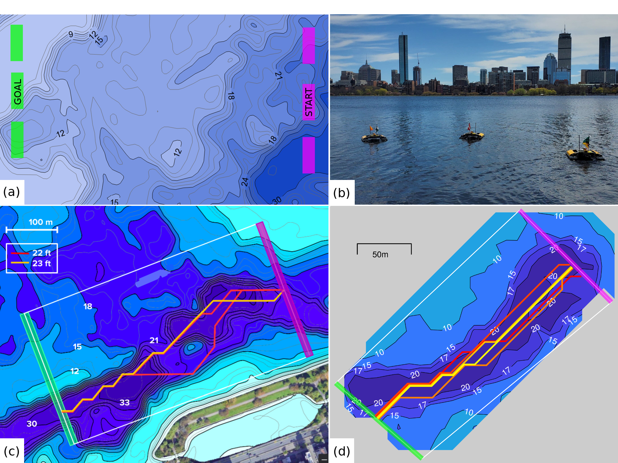
Figure 1: (a) Illustration of the rapid channel identification problem; quickly find a valid deep channel in an unknown environment that connects any of the start areas (magenta) to any of the goal areas (green). (b) Three of four Heron USVs equipped with low-cost single-beam sonar altimeters used for field testing. (c-d) Demonstration of our approach to find: (c) a channel deeper than 22ft and 23ft through the deep trench in the Charles River, and (d) a channel deeper than 17ft in Lake Popolopen in New York. The bathymetry map data for (a) and (c) is from [CRAB_Bathy]

The simplest way to survey an area is with a lawnmower search pattern. This is the most exhaustive method and will provide a comprehensive overview of the environment. However, for this problem, we are interested in finding a specific feature – a deep channel – rather than constructing a complete map. To speed up this process, we employ adaptive sampling strategies and robust multi-vehicle task allocation when more than one vehicle is available.

Using adaptive sampling and task allocation methods, we present the Proposal Based Adaptive Channel Search (PBACS) algorithm. To the best of the authors’ knowledge, we are the first to demonstrate a decentralized multi-vehicle approach to the channel identification problem, a unique but important challenge in marine engineering. The PBACS algorithm builds upon a combination of state-of-the-art methods in several areas: non-parametric environmental modeling (Fast Gaussian process regression (GPR) [das]) with decentralized bathymetry map fusion (modified decentralized Kalman consensus (MDKC) [alighanbari]), and multi-objective behavior optimization by interval programming (MOOS-IvP [benjamin])). The new PBACS algorithm employs an intuition regarding the structure of this particular type of exploration problem with directed search and market-based allocation in a way that outperforms other methods on average. Our approach is fully decentralized, and we have evidence that the advantages of the method can be realized with just one vehicle or with a cooperative group.

I-A Contributions

The contributions of this research are the following:

• The PBACS algorithm, a new specialized method for solving the rapid channel identification problem.

• Monte Carlo simulation studies to evaluate the utility of using different amounts of vehicles for PBACS, and to demonstrate better performance than both lawnmower and myopic Markov decision process (MDP) path planning.

• Multiple field deployments of the MDP approaches using up to three unmanned surface vehicles (USVs), and deployment of the PBACS approach using up to four USVs. Heron USVs made by Clearpath Robotics are shown in Figure 1b, and we report two successful demonstrations in the field where we found channels in the Charles River (Figure 1c) and Lake Popolopen in New York (Figure 1d).

II RELATED WORK

II-A Gaussian process (GP) and Path Planning

GPR is frequently used in marine adaptive sampling for spatial modeling of the estimated environment, which is then used to inform path planning. Berget et al. [berget] use GP methods to track suspended material plumes. The model is updated continuously throughout the mission, and the path planner uses this estimation to drive the unmanned vehicle to information-rich areas. In Fossum et al. [fossum], GP modeling is used for adaptive sampling of phytoplankton by modeling the distribution of chlorophyll-a - a common indicator of phytoplankton activity. Yan et al. [yan] use GPR analysis to guide online path planning for an AUV in an effort to locate hotspots in the field. Another work to use GP methods is Stankiewicz et al. [stankiewicz], where an AUV uses adaptive sampling to explore an area and identify hypoxic zones. The algorithm identifies regions of interest that exhibit some local extrema and concentrates sampling there.

II-B Classes of Adaptive Sampling Problems

Prior work in marine adaptive sampling can be separated into three broad categories: 1.) source localization methods as described by Bayat et al. in [bayat], which include gradient descent [paliotta] and partially observable Markov decision process (POMDP) [flaspohler], 2.) front/boundary determination, which have been demonstrated with single vehicles [zhang], [petillo15] and multiple vehicles [fiorelli2006multi], and 3.) feature tracking and mapping such as the work of Bennett et al. [bennett], where a simulated AUV is used to adaptively map bathymetric features like trenches or specific contours. Of these categories, the channel-finding problem explored in this paper is most closely related to the last, but is not specifically addressed in the literature.

II-C Multi-Vehicle Considerations

One of the main considerations in multi-vehicle missions is their formation. When the vehicles all explore the entire field, they can be in fixed formations such as in a leader-follower strategy employed by Khoshrou et al. [khoshrou] and Paliotta et al. [paliotta], or more flexible approaches such as generating different sailing directions for each vehicle, as proposed by Yan et al. in [yan].

When the field is explicitly divided, the divisions can either be predetermined or dynamic. An example of the latter is Kemna et al. [kemna], where dynamic Voronoi partitioning is used to divide the field among a group of AUVs. In general, flexible formations and dynamic divisions are more robust to single vehicle failures, which is part of the motivation for our approach.

Information sharing is a critical component of multi-vehicle systems, and communications can be range restricted or otherwise time-varying, especially in the marine domain. To address this problem, we use consensus protocols and algorithms for multi-vehicle coordination developed by Ren et al. [ren2] and Alighanbari et al. [alighanbari]. In particular, we use the robustness properties of the MDKC developed by Alighanbari et al. [alighanbari], which removes potential biases that occur when the agents in the network are not fully connected.

In many cases, vehicles need to coordinate new tasks/roles that arise as the mission progresses. One class of algorithms for solving this problem of task allocation is auction-based algorithms, also referred to as market-based algorithms. The implementations of these algorithms can rely upon a centralized repository, as described by Bertsekas [bertsekas]. They can also be distributed, as described by Michael et al. [michael] and Zavlanos et al. [zavlanos], which can be augmented with a consensus protocol to resolve conflicts [brunet2008consensus, raja2021communication].

II-D Multi-robot systems (MRS) for other applications

Recently, solutions to the general problem of collaborative exploration of an entire 3D map have been demonstrated with aerial vehicles [Tan2023RAL] and a mix of aerial and ground vehicles [CERBERUS20222]. However, our decentralized approach is designed to concentrate search in areas where a channel may still be viable. Furthermore, although the CERBERUS system in [CERBERUS20222] was the most successful in the DARPA Subterranean Challenge, the system used a centralized map server as the arbiter of information transmitted among the individual robots. Other decentralized approaches such as those reported in [Hou2022RAL] and [Toumieh2022RAL] use low-level control, which requires accurate models of the dynamics of each agent or conservative estimates that reduce optimality. In the case of marine vehicles, these models are more complex, and they operate in environments that are stochastic due to wind, waves, and currents [fossen2011handbook]. Due to these limitations, we instead implement multi-objective optimization via MOOS-IvP and control at the individual level. Finally, we emphasize our repeated experimental demonstrations of a multi-robot system in the field; the vehicles perform decentralized estimation and planning with limited computing power, low-cost single-beam sonars, and communication limitations.

III ENVIRONMENTAL MODELING

We represent the bathymetry data in a discrete set of $m$ grid-cells. We define the vectors $\vec{z}\in\rm I\!R^{m}$ and $\vec{\sigma}\in\rm I\!R_{+}^{m}$ as the depth and the variance (respectively) of each cell. The location of the center of the $i^{th}$ cell is denoted as $\vec{x}_{i}\in\rm I\!R^{2}$.

III-A Single-Beam Depth Sensor

We assume the depth directly below each vehicle can be measured by a single-beam acoustic depth sensor. For field work, we used the Ping Sonar Altimeter and Echosounder made by Blue Robotics for its low cost and commercial availability. A simulated sensor with comparable accuracy and noise was used for simulation studies.

The sensor was mounted onto the bottom plate of each Heron USV at the lowest possible depth that it remains submerged at all times without contacting the dock. The sensor was mounted directly below the GPS sensor in order to ensure that the distance readings are associated with the correct position. The sensor was then connected to the Heron’s payload autonomy computer and integrated into the MOOS system described in Section LABEL:section:implement_dets. We set the sampling rate of the sensor to 10 Hz.

III-B Efficient GPR

We use GPR on each vehicle to calculate an estimate for the bathymetry field within the grid from the collection of local measurements. The GPR implementation used in this system is adapted from the ”Fast GPR” developed by Das et al. [das]. The Fast GPR aims to speed up computation by developing estimators on subsets of the dataset. Using the standard implementation of GPR on a dataset of size $N$ yields $O(N^{3})$ time complexity. By choosing $k$ subsets of size $N_{s}<N$, the time complexity of Fast GPR is reduced to $O(kN_{s}^{3})$. One limitation of this method is that the variance becomes skewed, but we address this minor complication in Section IV-B with the threshold in (5).

We use the Gaussian kernel

$$\mathcal{K}(\vec{x}_{i},\vec{x}_{j})=exp\Big{(}-\frac{d(\vec{x}_{i},\vec{x}_{j})}{2l^{2}}\Big{)},$$ (1)

where $d(\vec{x}_{i},\vec{x}_{j})$ is the Euclidean distance. We determined experimentally that $l\approx 28.8ft$ works well in field testing.

III-C Decentralized Map Fusion

For multi-vehicle coordination, we use the Modified Decentralized Kalman Consensus (MDKC) reported by Alighanbari and How [alighanbari]. Although we extensively test our approach with USVs that can more easily communicate, our approach is intended to be used in multi-vehicle systems that include unmanned underwater vehicles (UUVs), which have limited communications while submerged. For that reason, we use a periodic consensus to combine estimates of the map from each vehicle in a way that requires limited communication bandwidth, works without a fully connected communications graph, and is robust to intermittent communication failures.

A consensus can be reached even if the group does not form a fully connected graph, which happened periodically during field operations as vehicles temporarily drop out of communication.

For $n$ agents $\mathcal{A}=\{\mathcal{A}_{i},...,\mathcal{A}_{n}\}$, the solution for an agent $\mathcal{A}_{i}$ at time $t+1$ is given by:

$$\bm{P_{i}}(t+1)= \{[\bm{P_{i}}(t)+\bm{Q}(t)]^{-1}$$

$$+\sum_{j=1}^{n}(g_{ij}(t)[\mu_{j}(t)\bm{P_{j}}(t)]^{-1})\}^{-1}$$ (2)

$$\vec{z}_{i}(t+1) =\vec{z}_{i}(t)$$

$$+\bm{P_{i}}(t+1)\sum_{j=1}^{n}\{g_{ij}(t)\cdot[\mu_{j}(t)\bm{P_{j}(t)}]^{-1}$$

$$\cdot(\vec{z}_{j}(t)-\vec{z}_{i}(t))\}$$ (3)

$$\mu_{j}(t)=\sum_{k=1,k\neq j}^{n}g_{kj}(t)$$ (4)

where $\bm{P_{i}}$ is the covariance matrix assembled using the radial basis function kernel (1) and the grid variance $\vec{\sigma}$, $\bm{Q}(t)$ is the process noise (used only when a vehicle becomes completely disconnected and must complete the consensus on their own), $\vec{z}_{i}$ is the agent’s own information, $g_{ij}$ is the adjacency matrix of the communication graph between agents $\mathcal{A}_{i}$ and $\mathcal{A}_{j}$, and $\mu_{j}(t)$ is a scaling factor associated with agent $\mathcal{A}_{j}$.

IV CHANNEL SEARCH

Here we present our main algorithm, a more specialized method for solving the channel identification problem. There are two stages to this approach: an exploratory sweep and a search along candidate paths. A simplified version of the process is illustrated in Figure 2, and the proposal algorithm is reproduced in Algorithm LABEL:algo::PBACS.

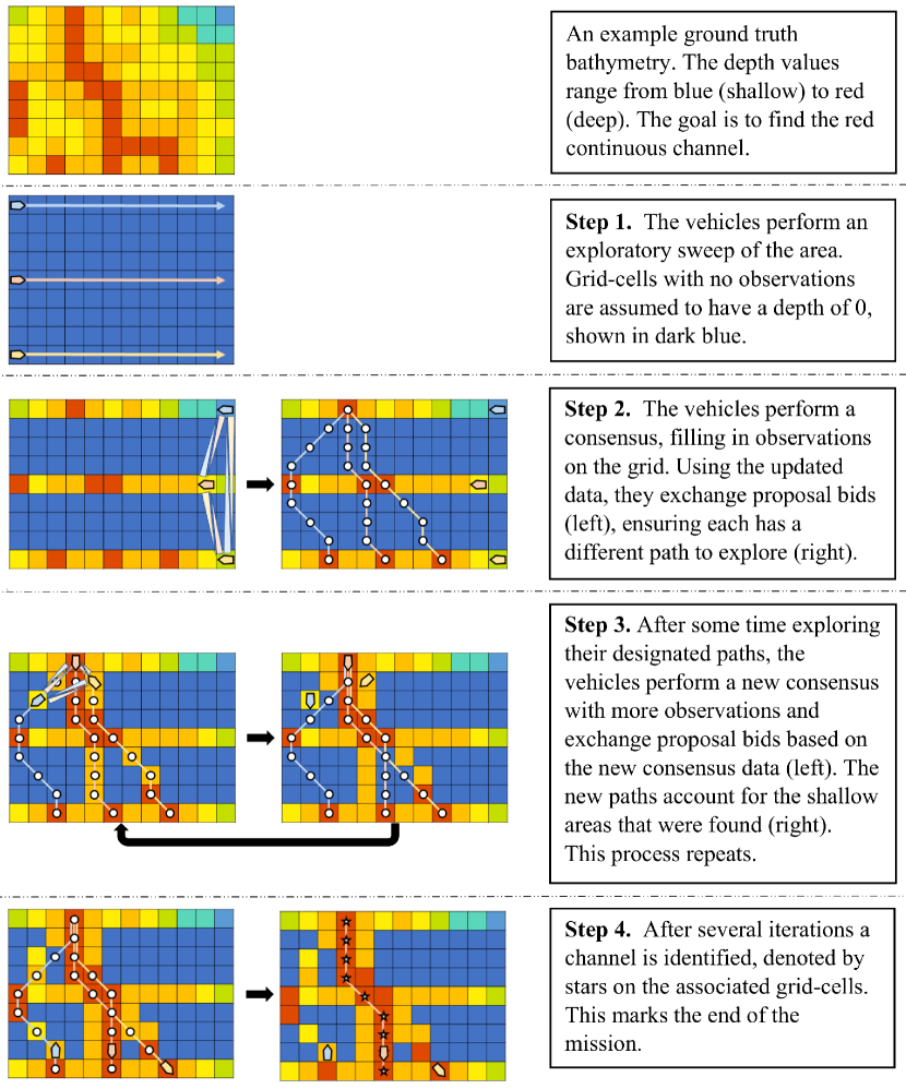
Figure 2: The simplified steps of PBACS.

IV-A First Stage - Exploratory Sweep

The first stage of PBACS is an exploratory sweep of the area. Other adaptive sampling works have also employed an initial exploratory lawnmower sweep to seed the remainder of the search [bennett], [paliotta]. For our problem, we can use such a sweep to help save time by eliminating areas that do not meet the necessary depth criteria, thereby directing the search toward more likely channel regions (Step 1 in Figure 2). For a single-vehicle mission we set the initial sweep to cover the start area of the grid, and for a two-vehicle mission we cover the start and end goal areas. The sweep area for each subsequent vehicle is an equally spaced line in between.

IV-B Second Stage - Path Exploration

The second stage after the sweep is the path exploration stage, shown in Algorithm LABEL:algo::PBACS. Vehicles enter this stage after they complete their initial sweep, and this transition often occurs asynchronously due to the difference in transit times to the initial sweep locations.

The goal of this stage is to identify and explore candidate paths that may still be viable. Each vehicle proposes a path between the start and goal regions that may be part of a viable channel (Step 2 in Figure 2). These candidate paths can be generated using any path planner; here we used a common variant of the A* planner which searches for a path that connects any of several start and goal locations.

The depth along a candidate path must not be shallow, and we capture this criterion in our search problem with simulated obstacles. Grid-cells are considered obstacles only if they have a sufficiently low variance and are too shallow. This way, candidate paths are made up of cells that are either certainly deep enough, or that we are uncertain about how deep they actually are. The variance threshold for considering a shallow grid-cell to be an obstacle is calculated dynamically as a percentage of the range between the current minimum and maximum variance across the grid, i.e.

$$\sigma_{th}=\sigma_{min}+\eta(\sigma_{max}-\sigma_{min}).$$ (5)

where the probability distribution is computed using the MDKC algorithm as described in Section III-C. This threshold must be set high enough to exclude shallow grid-cells with low variance, typically those that have been directly measured by at least one vehicle. The threshold should also be low enough to not exclude shallow grid-cells with high variance, typically those that were interpolated. We experimentally determined $\eta=0.33$ to be sufficient for both simulation and fieldwork.

Upon completion of each GPR estimate and consensus, the path is rechecked to ensure that no new obstacles were found on it and that it is still optimal (Steps 2 and 3 in Figure 2). If a more optimal and obstacle-free path is found, the vehicle switches to this path (Step 3 in Figure 2). We periodically check for the existence of a valid continuous channel, which marks the end of the mission (Step 4 in Figure 2).