Comparing Shape-Constrained Regression Algorithms for Data Validation

Abstract

Industrial and scientific applications handle large volumes of data that render manual validation by humans infeasible. Therefore, we require automated data validation approaches that are able to consider the prior knowledge of domain experts to produce dependable, trustworthy assessments of data quality. Prior knowledge is often available as rules that describe interactions of inputs with regard to the target e.g. the target must be monotonically decreasing and convex over increasing input values. Domain experts are able to validate multiple such interactions at a glance. However, existing rule-based data validation approaches are unable to consider these constraints. In this work, we compare different shape-constrained regression algorithms for the purpose of data validation based on their classification accuracy and runtime performance.

1 Introduction

Modern applications record a staggering amount of data through the application of sensor platforms. These masses of data render manual validation infeasible and require automated data validation approaches. Existing rule-based approaches [5] can detect issues like missing values, outliers, or changes in the distribution of individual observables. However, they are unable to assess the data quality based on interactions of multiple observables with regard to a target. For example, they might falsely classify an outlier as invalid, even though it can be explained by changes in another variable. Alternatively, an observable might exhibit valid value ranges and distributions, whilst the error is only detectable in the unexpected interaction with other observables, e.g. one dependent variable remains of constant value while another changes.

For this purpose, we propose the use of shape constraints (SC) for data validation. We detail the general idea of SC-based data validation and provide a comparison of three algorithms: (1) shape-constrained polynomial regression (SCPR) [8], (2) shape-constrained symbolic regression (SCSR) [9, 2] and (3) eXtreme gradient boosting (XGBoost) [3]. We compare classification accuracy, supported constraint types, and runtime performance based on data stemming from a use-case in the automotive industry.

2 SC-based data validation

ML algorithms have long been applied for the purpose of data validation. Concept drift detection [6] applies e.g. ML models and analyzes the prediction error to detect changes in system behavior. These models are either trained on data from a manually validated baseline and detect subsequent deviations from this established baseline, or are trained continuously to detect deviations from previous states [7]. SC-based data validation, however, is able to assess the quality of unseen data without established baselines by using domain knowledge.

Quality of data is often assessed by analysis of the interaction of inputs values in regard to the target. The measured target must exhibit certain shape properties that we associate with valid data and valid interactions. SCR allows us to train prediction models on the potentially erroneous dataset, whilst enforcing a set of shape constraints. Therefore, the trained prediction model exhibits a higher error if the data contains outliers or erroneous segments that violate the provided constraints, as SCR is restricting the model from fitting to these values.

Figure 1: Over-simplified showcase of SC-based data validation. The constrained model $f_{2}$ exhibits a higher error as it is restricted from fitting to certain data points, but it exhibits the monotonicity of the generating base function.

Figure 1 shows a simplified example where we sample training data from a third degree polynomial base function $f$, with added normally distributed noise. Subsequently, we train the linear factors $\overrightarrow{\theta}$ of two third degree polynomials, with and without constraints. The constrained model $f_{2}$ exhibits a higher training error as it includes no decreasing area $x\in[-1,1]$ visible in $f_{1}$, but exhibits the monotonicity of the generating function as enforced by the constraints.

SC-based data validation requires two prerequisites: (1) precise constraints that describe valid system behavior and (2) a small set of manually validated data. These manually validated datasets are required to perform a one-time grid search to determine the best algorithm parameters for each application scenario. Later, for all arriving unseen datasets, a constrained model is trained on the full data. Similar to Figure 1, datasets are labeled as invalid when the model exhibits a high training error and exceeds a threshold $t$.

3 Shape-Constrained Regression (SCR)

Shape-constrained regression (SCR) allows the enforcement of shape-properties of the regression models. Shape-properties can be expressed as restrictions on the partial derivatives of the prediction model that are defined for a range of the input space. This side information is especially useful when training data is limited. The combination of data with prior knowledge can increase trust in model predictions[4], which is an equally important property in data validation. Table 1 lists common examples of shape constraints together with the mathematical expression and compares the capabilities of the different algorithms.

3.1 Shape-Constrained Polynomial Regression (SCPR)

For regular polynomial regression (PR), a parametric (multi-variate) polynomial is fit to data. This is achieved by fitting the linear coefficients of each term using ordinary least squares (OLS). For SCPR, we include sum-of-squares constraints (a relaxation of the shape constraints) to the OLS objective function, which leads to a semidefinite programming problem (SDP) [10]. We use the commercial solver Mosek to solve the second-order cone problem (SOCP) without shape constraints and the SDP with shape constraints. The algorithm parameters of PR and SCPR are: $d$ the (total) degree of the polynomial, $\lambda$ the strength of regularization, and $\alpha$ used to balance between 1-norm (lasso regression) and 2-norm (ridge regression) penalties. SCPR is able to incorporate all constraints of Table 1, is deterministic and produces reliable results in relatively short runtime.

3.2 Shape-constrained symbolic regression (SCSR)

SCSR [9] uses a single objective genetic algorithm (GA) to train a symbolic regression model. After evaluation, in an additional model selection step, the constraints are asserted by calculating the prediction intervals on partial derivatives of the model. Any prediction model that violates a constraint is assigned the error of the worst performing individual, thereby preserving genetic material. Due to the probabilistic nature of the GA the achievement of constraints is not guaranteed.

3.3 XGBoost - eXtreme Gradient Boosting

XGBoost [3] builds an ensemble of decision trees with constant valued leaf nodes. It is able to consider monotonic constraints, however, these constraints can only be enforced on the whole input space of one input vector $\overrightarrow{x_{i}}$. It provides no support for larger intervals (extrapolation guidance), or multiple (overlapping) constraint intervals, like SCPR or SCSR. This results in fewer, less specific constraints available for XGBoost as summarized Table 1. XGBoost uses the parameters $\lambda$, $\alpha$ to determine the 1-norm (lasso regression) and 2-norm (ridge regression) penalties respectively.

Table 1: Examples of shape constraints. All constraints marked with $\bullet$ are enforced for a domain $[l_{i},u_{i}]\subseteq\overrightarrow{x_{i}}$ of the full $\overrightarrow{x_{i}}$ input space. Multiple constraints can be defined over several partitions. Constraints for algorithms marked with $\ast$, however, can only be asserted on the full input space of $\overrightarrow{x_{i}}$. Constraints marked with $\circ$ are not available.

Property	Mathematical formulation	SCPR	SCSR	XGBoost
Positivity	$f(X)\geq 0$	$\bullet$	$\bullet$	$\circ$
Negativity	$f(X)\leq 0$	$\bullet$	$\bullet$	$\circ$
Monotonically increasing	$\frac{\partial}{\partial x_{i}}f(X)\geq 0$	$\bullet$	$\bullet$	$\ast$
Monotonically decreasing	$\frac{\partial}{\partial x_{i}}f(X)\leq 0$	$\bullet$	$\bullet$	$\ast$
Convexity	$\frac{\partial^{2}}{\partial x_{i}^{2}}f(X)\geq 0$	$\bullet$	$\bullet$	$\circ$
Concavity	$\frac{\partial^{2}}{\partial x_{i}^{2}}f(X)\leq 0$	$\bullet$	$\bullet$	$\circ$

4 Experiment and Setup

This section provides a short description of the data from our real-world use-case and discusses the experiment setup used to compare the investigated SCR algorithms based on this use-case. We follow the general description of SC-based data validation as described in Section 2.

4.1 Problem Definition - Data from Friction Experiments

Miba Frictec GmbH develops friction systems such as breaks or clutches for the automotive industry. The exact friction characteristics of novel material compositions are unknown during development, and can only be determined by time- and resource-intense experiments. For this purpose, a friction disc prototype is installed in room filling test-rigs that rotate the discs at different velocities $v$, and repeatedly engage the discs at a varying pressure $p$ to simulate the actuation of a clutch during shifting. Based on these measurements, the friction characteristics of new discs are determined. The friction coefficient $\mu$ denotes the ratio of friction force and normal load. It describes the force required to initiate and to maintain relative motion (denoted static friction $\mu_{\textit{stat}}$ and dynamic friction $\mu_{\textit{dyn}}$) [1]. The value of $\mu$ is not constant for one friction disc, instead, it is dependent on the parameters: $p$, $v$ and temperature $T$. Experts determine the quality of data by analyzing the interactions of $p,v,T$ with regard to $\mu_{\textit{dyn}}$.

In friction experiments we encounter several known issues that render whole datasets or segments erroneous and that are only detectable when we investigate the interaction of inputs with regard to the target $\mu_{\textit{dyn}}$. Examples for such errors include: wrong calibration or malfunction of sensors, loosened or destroyed friction pads, or contaminated test benches from previous failed experiments. We were provided a total of 53 datasets consisting of 18 manually validated and 35 known invalid datasets that were annotated with a description of the error type.

$$\forall_{v,p,T}\hskip 5.0ptv\in[0,1]\wedge p\in[0,1]\wedge T\in[0,1]\implies$$

$$\Big{(}0\leq\mu_{\textit{dyn}}\leq 1\wedge\frac{\partial\mu_{\textit{dyn}}}{\partial v}\in[-0.01,0.01]$$

$$\wedge\frac{\partial\mu_{\textit{dyn}}}{\partial p}\leq 0\wedge\frac{\partial^{2}\mu_{\textit{dyn}}}{\partial p^{2}}\geq 0\wedge\frac{\partial\mu_{\textit{dyn}}}{\partial T}\leq 0\wedge\frac{\partial^{2}\mu_{\textit{dyn}}}{\partial T^{2}}\geq 0\Big{)}$$ (1)

$$\forall_{p,T}\hskip 5.0ptp\in[0,1]\wedge T\in[0,1]\implies\Big{(}\frac{\partial\mu_{\textit{dyn}}}{\partial p}\leq 0\wedge\frac{\partial\mu_{\textit{dyn}}}{\partial T}\leq 0\Big{)}$$ (2)

4.2 Experiment Setup

We performed a hyper-parameter search using a two-fold cross validation over all valid datasets, repeated for each algorithm. As the constraints define expected behavior, each algorithm should be able to train models with low test error on valid data, whilst adhering to the constraints. Equation 4.1 lists the constraints for $\mu_{\textit{dyn}}$, which were provided by domain experts. Inputs $p,v,T$ are individually scaled to a range of $[0,1]$ and all constraints are defined for this full input space. Equation 2 lists the reduced constraints that are compatible with XGBoost’s capabilities.

Figure 2: Grid search results for SCPR over all validated datasets. Lower values signify better results.

Figure 2 visualizes the search space and best configuration for SCPR in a heatmap showing the sum of test RMSE over all valid datasets. Similar experiments and analysis were conducted for PR and XGBoost. For SCSR, we compared training and test error over increasing generation count. To prevent overfitting we select the generation with the lowest test error as a stopping criterion. In all subsequent training on unseen data, during the validation phase, the GA is stopped at this generation.

The resulting best SCR algorithm parameters were applied in the SC-based data validation phase for all available datasets. In this use-case, we divide the dataset into a new segment when one of the controlled input parameters $p$ or $v$ changed (cf. Figure 3). We calculate the RMSE values per segment and mark the whole experiment as invalid if one segment exceeds the varied threshold $t$.

Figure 3: Validation result for data of one friction experiment. SC-based data validation was able to detect the subtle deviations from expected behavior in the segments one and five with row IDs 0-25, 100-125. The drops in $\mu_{\textit{dyn}}$-measured are not motivated by the friction dynamics. This dataset was correctly labeled invalid.

5 Results

A comparison of the investigated SCR algorithms is visualized in Figure 4. XGBoost supports fewer, less complex shape constraints and achieves only minimally better classification capabilities than the unrestricted PR baseline. The comparison with PR shows how many erroneous datasets are simply detectable due to the statistical properties of ML models. The objective function of minimized training error leads to models being fit to the behavior represented in the majority of the data, resulting in the detection of less represented behavior or outliers. SCPR and SCSR on the other hand exhibit significantly improved classification capabilities, which can be attributed to the increased restrictions added by the constraints and domain knowledge about expected valid behavior.

We subsequently varied the threshold value $t$ to analyze the change in false-positive- and true-positive-rate as visualized Figure 4. Higher values of $t$ result in the detection of only severe errors and a lower false positives rate. Lower values of $t$ cause a more sensitive detection and higher false positive rates.

The sharp vertical incline in the ROC-curve of Figure 4 is caused by the numerous invalid datasets that exhibit severe errors like e.g. massive outliers. Such errors cause high training error regardless if constraints are applied and how restrictive they are. Eventually, for increasingly smaller values of $t$, even noise present in the data will result in a training error that exceeds $t$.

Figure 4 also compares the test RMSE values achieved by the best algorithm parameters on the 18 valid datasets. All three algorithms are similarly well suited for modeling friction data. Consequently, all conclusions about the data validation capabilities of individual algorithms are not biased by the training accuracy. With an average training time of 0.32s per dataset and great classification capabilities, SCPR is best suited for SC-based data validation. In practical applications, the data quality assessment is implemented in automated data ingestion pipelines that require low latencies. SCPR adds only little in terms of computational effort but provides significant improvement in data quality.

(a) Receiver operator characteristics (ROC) curve, showing the classification capabilities.

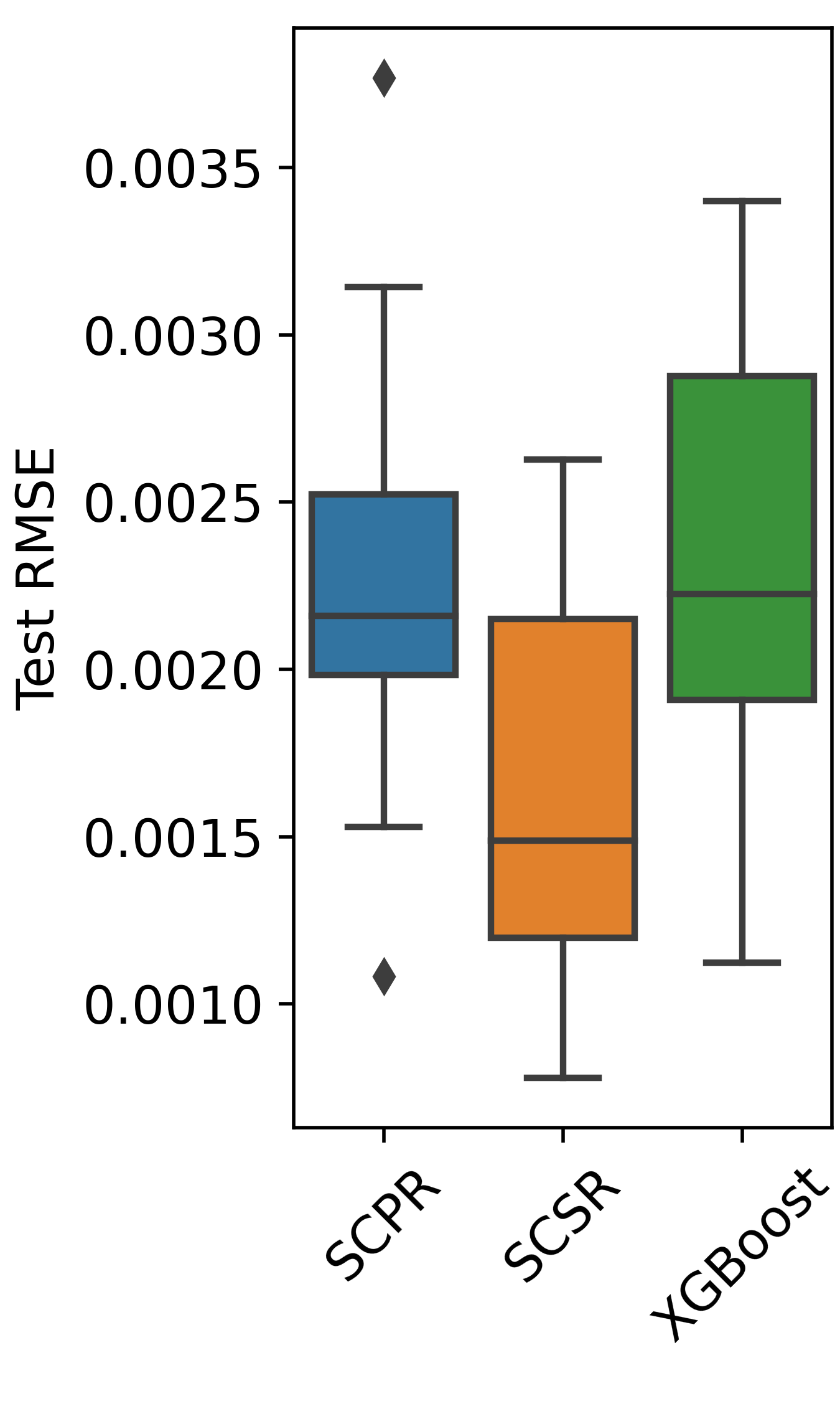
(b) Grid search test error.

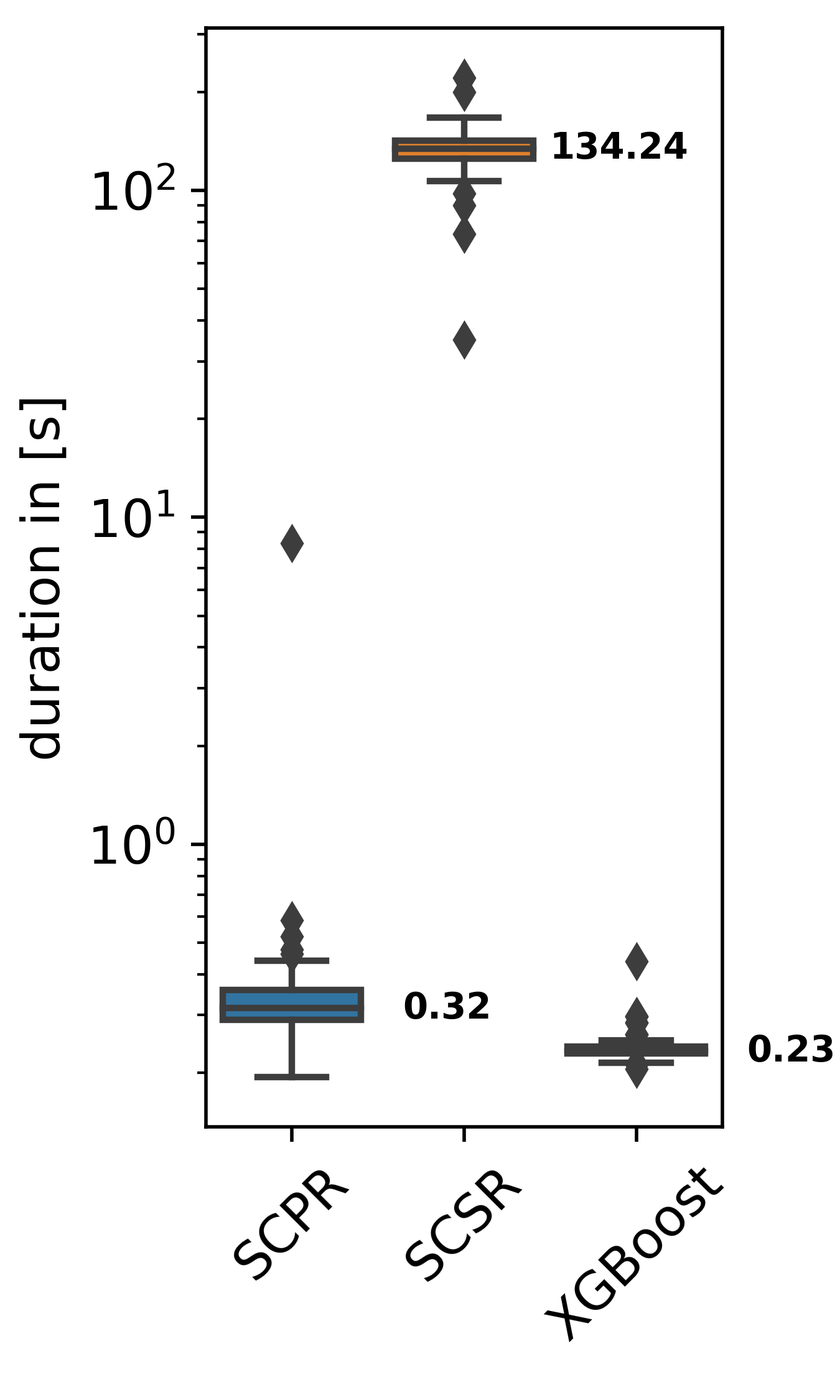
(c) Training duration.

Figure 4: Performance comparison of the three SCR algorithms and unconstrained PR.

6 Conclusions

SC-based data validation is a novel approach that allows the inclusion of prior knowledge in the quality assessment of previously unseen datasets. It can detect faults in the data that are only identifiable in the interaction of observables. With its low average runtime, SC-based data validation using SCPR is suitable for integration into data import pipelines to improve data quality. Moreover, trust in the validation results is facilitated by readable constraint definitions that can be provided by domain experts, or derived from expert knowledge. This trust is further increased through interpretable models created by the white- or gray-box ML algorithms SCPR and SCSR.

Based on our experiments, we recommend the application of SCPR for SC-based data validation. SCPR is easy to configure and excels in runtime time performance, as well as classification accuracy. For cases with larger number of variables or categorical data, XGBoost might be better equipped.

Acknowledgement

The financial support by the Christian Doppler Research Association, the Austrian Federal Ministry for Digital and Economic Affairs and the National Foundation for Research, Technology and Development is gratefully acknowledged.

References

- [1] Bhushan, B.: Introduction to Tribology, chap. Friction, pp. 199–271. John Wiley & Sons, Ltd (2013), https://onlinelibrary.wiley.com/doi/abs/10.1002/9781118403259.ch5
- [2] Bladek, I., Krawiec, K.: Solving symbolic regression problems with formal constraints. In: Proceedings of the Genetic and Evolutionary Computation Conference. p. 977–984. GECCO ’19, Association for Computing Machinery, New York, NY, USA (2019). https://doi.org/10.1145/3321707.3321743
- [3] Chen, T., Guestrin, C.: Xgboost: A scalable tree boosting system. In: Proceedings of the 22nd ACM SIGKDD International Conference on Knowledge Discovery and Data Mining. p. 785–794. KDD ’16, Association for Computing Machinery, New York, NY, USA (2016). https://doi.org/10.1145/2939672.2939785
- [4] Cozad, A., Sahinidis, N.V., Miller, D.C.: A combined first-principles and data-driven approach to model building. Computers & Chemical Engineering 73, pp. 116–127 (2015)
- [5] Ehrlinger, L., Wöß, W.: A survey of data quality measurement and monitoring tools. Frontiers in Big Data p. 28 (2022), https://doi.org/10.3389/fdata.2022.850611
- [6] Gama, J., Medas, P., Castillo, G., Rodrigues, P.: Learning with drift detection. In: Brazilian symposium on artificial intelligence. pp. 286–295. Springer (2004)
- [7] Gama, J., Žliobaitė, I., Bifet, A., Pechenizkiy, M., Bouchachia, A.: A survey on concept drift adaptation. ACM Comput. Surv. 46(4) (Mar 2014). https://doi.org/10.1145/2523813
- [8] Hall, G.: Optimization over Nonnegative and Convex Polynomials With and Without Semidefinite Programming. Ph.D. thesis, Princeton University (2018)
- [9] Kronberger, G., de Franca, F.O., Burlacu, B., Haider, C., Kommenda, M.: Shape-Constrained Symbolic Regression—Improving Extrapolation with Prior Knowledge. Evolutionary Computation 30(1), 75–98 (03 2022), https://doi.org/10.1162/evco_a_00294
- [10] Parrilo, P.A.: Structured semidefinite programs and semialgebraic geometry methods in robustness and optimization. Ph.D. thesis, California Institute of Technology (2000)