Polynomial-Time Reachability for LTI Systems with Two-Level Lattice Neural Network Controllers

Abstract

In this paper, we consider the computational complexity of bounding the reachable set of a Linear Time-Invariant (LTI) system controlled by a Rectified Linear Unit (ReLU) Two-Level Lattice (TLL) Neural Network (NN) controller. In particular, we show that for such a system and controller, it is possible to compute the exact one-step reachable set in polynomial time in the size of the TLL NN controller (number of neurons). Additionally, we show that a tight bounding box of the reachable set is computable via two polynomial-time methods: one with polynomial complexity in the size of the TLL and the other with polynomial complexity in the Lipschitz constant of the controller and other problem parameters. Finally, we propose a pragmatic algorithm that adaptively combines the benefits of (semi-)exact reachability and approximate reachability, which we call L-TLLBox. We evaluate L-TLLBox with an empirical comparison to a state-of-the-art NN controller reachability tool. In our experiments, L-TLLBox completed reachability analysis as much as 5000x faster than this tool on the same network/system, while producing reach boxes that were from 0.08 to 1.42 times the area.

I Introduction

Neural Networks (NNs) are increasingly used to control dynamical systems in safety critical contexts. As a result, the problem of formally verifying the safety properties of NN controllers in closed loop is a crucial one. Despite this, comparatively little attention has been paid to the time-complexity of such reachability analysis. Understanding – and improving – the complexity of NN verification algorithms is thus crucial to designing provably safe NN controllers: it bears directly on the size of NNs that can be pragmatically verified.

Formal verification of NNs is usually formulated in terms of static input-output behavior, but there are few results analyzing the time complexity of such input-output verification [9, 6, 12]. We know of no paper that directly analyzes the time-complexity of exact reachability analysis for LTI systems with NN controllers, although [11] comes closest. Note: exact reachability is distinct from (polynomial-time) set-based reachability methods, which consider an over-approximated set of possible controller outputs in each state [2]. Formally, [11] only provides a complexity result for verifying the input-output behavior of a NN, but the underlying methodology, star sets, suggests a complexity analysis for exact reachability of LTI systems. Unfortunately, that algorithm produces exponentially many star sets – in the number of neurons – just to verify the input-output behavior of a NN once [11, Theorem 1]; this exponential complexity compounds with each additional time step in reachability analysis. No such analysis is provided for the accompanying approximate star-set reachability analysis.

In this paper, we show that for a certain class of ReLU NN controllers – viz. Two-Level Lattice (TLL) NNs [5] – exact (or quantifiably approximate) reachability analysis for a controlled discrete-time LTI system is worst-case polynomial time complexity in the size (number of neurons) of the TLL NN controller. Thus, we show that LTI reachability analysis for the TLL NN architecture is dramatically more efficient (per neuron) than the same problem with general NNs (i.e. exponential complexity [11]; see above). In this sense, our results motivate for directly designing TLL NN controllers in the first place, since reachability for a TLL NN controller is more efficient to compute (TLL NNs are similarly beneficial in other problems: e.g. verification [4]). Moreover, TLL NNs can realize the same functions that general ReLU NNs can, so no generality in realizable controllers is lost by this choice.

In particular, we prove several polynomial-complexity results related to the one-step reachable set of a discrete-time LTI system: i.e., the set $X_{t+1}=\{Ax+B{\mathscr{N}\negthickspace\negthickspace\negthinspace\mathscr{N}}\negthinspace(x)|x\in X_{t}\}$ for a given polytopic set of states $X_{t}$ and a TLL controller ${\mathscr{N}\negthickspace\negthickspace\negthinspace\mathscr{N}}\negthinspace$. Moreover, we consider the computation of both the exact set $X_{t+1}$ and an $\epsilon$-tight bounding box of $X_{t+1}$. All claimed complexities are worst case and with respect to a fixed state-space dimension, $n$. These results are summarized as:

1. The exact one-step reachable set, $X_{t+1}$, can be computed in polynomial time-complexity in the size of the TLL NN (Theorem 1).

2. An $\epsilon$-tight bounding box for $X_{t+1}$ can be computed via three algorithms with time-complexities:

   1. polynomial in size of the TLL (Theorem 2); or

   2. polynomial in the Lipschitz constant of the controller, the accuracy, $\epsilon$, the norm of the $B$ matrix and the volume of $X_{t}$ (Proposition 1); or

   3. the minimum complexity of (ii-a) and (ii-b) (Theorem 3); this uses polynomial-time Lipschitz constant computation for TLLs (Lemma 1).

Here an $\epsilon$-tight bounding box of $X_{t+1}$ is one that is within $\epsilon>0$ of the exact, coordinate-aligned bounding box of $X_{t+1}$.

In addition, we propose an algorithm that adaptively combines notions of exact and approximate bounding box reachability for TLL NNs in order to obtain an extremely effective approximate reachability algorithm, which we call L-TLLBox. We validate this method by empirically comparing an implementation of L-TLLBox with the state-of-art NN reachability tool, NNV [12]. On a test suite of TLL NNs derived from the TLL Verification Benchmark in the 2022 VNN Competition [1], L-TLLBox performed LTI reachability analysis as much as 5000x faster than NNV on the same reachability problem; L-TLLBox produced reach boxes of 0.08 to 1.42 times the area produced by NNV.

Related work: There is a large literature on the complexity of set-based reachability for LTI systems; [2] provides a good summary. For the complexity of LTI-NN reachability, [11] is the closest to providing an explicit, exact result. The complexity of approaches based NN over-approximation have been considered in [7, 8]. The literature on the complexity of input-output verification of NNs is larger but still small: [11] falls in this category as well; [9] is important for its NP-completeness result based on the 3-SAT encoding; and [6, 4] consider the complexity of verifying TLL NNs. Other NN-related complexity results include: computing the minimum adversarial disturbance is NP hard [14], and computing the Lipschitz constant is NP hard [13].

II Preliminaries

II-A Notation

We will denote the real numbers by $\mathbb{R}$. For an $(n\times m)$ matrix (or vector), $A$, we will use the notation $\llbracket A\rrbracket_{[i,j]}$ to denote the element in the $i^{\text{th}}$ row and $j^{\text{th}}$ column of $A$. Analogously, the notation $\llbracket A\rrbracket_{[i,:]}$ will denote the $i^{\text{th}}$ row of $A$, and $\llbracket A\rrbracket_{[:,j]}$ will denote the $j^{\text{th}}$ column of $A$; when $A$ is a vector instead of a matrix, both notations will return a scalar corresponding to the corresponding element in the vector. We will use angle brackets $\;\negthinspace\text{{\stixfrak\char 54\relax}}\cdot\text{{\stixfrak\char 55\relax}}$ to delineate the arguments to a function that returns a function. We use one special form of this notation: for a function $f:\mathbb{R}^{n}\rightarrow\mathbb{R}^{m}$ and $i\in\{1,\dots,m\}$ define $\pi_{i}\negthinspace\text{{\stixfrak\char 54\relax}}f\text{{\stixfrak\char 55\relax}}:x\mapsto\llbracket f(x)\rrbracket_{[i,:]}$. Finally, $\lVert\cdot\rVert$ will refer to the max-norm on $\mathbb{R}^{n}$, unless otherwise specified.

II-B Neural Networks

We consider only Rectified Linear Unit Neural Networks (ReLU NNs). A $K$-layer ReLU NN is specified by $K$ layer functions; a layer may be either linear or nonlinear. Both types of layer are specified by a parameter list $\theta\triangleq(W,b)$ where $W$ is a $(\overline{d}\times\underline{d})$ matrix and $b$ is a $(\overline{d}\times 1)$ vector. Specifically, the linear and nonlinear layers specified by $\theta$ are denoted by $L_{\theta}$ and $L_{\theta}^{\scriptscriptstyle\sharp}$, respectively, and are defined as:

$$L_{\theta} :\mathbb{R}^{\scriptscriptstyle\underline{d}}\rightarrow\mathbb{R}^{\scriptscriptstyle\overline{d}}, L_{\theta} :z\mapsto Wz+b$$ (1)

$$L_{\theta}^{\scriptscriptstyle\sharp} :\mathbb{R}^{\scriptscriptstyle\underline{d}}\rightarrow\mathbb{R}^{\scriptscriptstyle\overline{d}}, L_{\theta}^{\scriptscriptstyle\sharp} :z\mapsto\max\{L_{\theta}(z),0\}.$$ (2)

where the $\max$ function is taken element-wise. Thus, a $K$-layer ReLU NN function is specified by functionally composing $K$ such layer functions whose parameters $\theta^{|i},i=1,\dots,K$ have dimensions that satisfy $\underline{d}^{|i}=\overline{d}{\vphantom{d}}^{|i-1}:i=2,\dots,K$; we will consistently use the superscript notation ^|k to identify a parameter with layer $k$. Whether a layer function is linear or not will be further specified by a set of linear layers, $\mathtt{lin}\subseteq\{1,\dots,K\}$. For example, a typical $K$-layer NN has $\mathtt{lin}=\{K\}$, which together with a list of $K$ layer parameters defines the NN: ${\mathscr{N}\negthickspace\negthickspace\negthinspace\mathscr{N}}\negthinspace=L_{\theta^{|K}}^{\vphantom{{\scriptscriptstyle\sharp}}}\circ L_{\theta^{|K-1}}^{\scriptscriptstyle\sharp}\circ\dots\circ L_{\theta^{|1}}^{\scriptscriptstyle\sharp}$.

To indicate the dependence on parameters, we will index a ReLU ${\mathscr{N}\negthickspace\negthickspace\negthinspace\mathscr{N}}\negthinspace$ by a list of NN parameters $\Theta\triangleq$ $(\mathtt{lin},\theta^{|1},$ $\dots,$ $\theta^{|K});$ i.e., we will often write ${\mathscr{N}\negthickspace\negthickspace\negthinspace\mathscr{N}}\negthinspace\negthinspace\text{{\stixfrak\char 54\relax}}\Theta\text{{\stixfrak\char 55\relax}}:\mathbb{R}^{\scriptscriptstyle\underline{d}\vphantom{d}^{|1}}\rightarrow\mathbb{R}^{\scriptscriptstyle\overline{d}\vphantom{d}^{|K}}$.

II-C Two-Level-Lattice (TLL) Neural Networks

In this paper, we consider only Two-Level Lattice (TLL) ReLU NNs. Thus, we formally define NNs with the TLL architecture using the succinct method exhibited in [6]; the material in this subsection is derived from [5, 6].

A TLL NN is most easily defined by way of three generic NN composition operators. Hence, the following three definitions lead to the TLL NN in Definition 4.

Definition 1 (Sequential (Functional) Composition).

Let ${\mathscr{N}\negthickspace\negthickspace\negthinspace\mathscr{N}}\negthinspace\negthinspace\text{{\stixfrak\char 54\relax}}\Theta_{\scriptscriptstyle i}\text{{\stixfrak\char 55\relax}}:\mathbb{R}^{\underline{d}^{\scriptscriptstyle|1}_{i}}\rightarrow\mathbb{R}^{\overline{d}\vphantom{d}^{|K_{i}}_{i}}$, $i=1,2$ be two NNs with parameter lists $\Theta_{i}\triangleq(\mathtt{lin}_{i},\theta^{\scriptscriptstyle|1}_{i},\dots,\theta^{\scriptscriptstyle|K_{i}}_{i})$, $i=1,2$ such that $\overline{d}\vphantom{d}^{\scriptscriptstyle|K_{1}}_{1}=\underline{d}^{\scriptscriptstyle|1}_{2}$. Then the sequential (or functional) composition of ${\mathscr{N}\negthickspace\negthickspace\negthinspace\mathscr{N}}\negthinspace\negthinspace\text{{\stixfrak\char 54\relax}}\Theta_{\scriptscriptstyle 1}\text{{\stixfrak\char 55\relax}}$ and ${\mathscr{N}\negthickspace\negthickspace\negthinspace\mathscr{N}}\negthinspace\negthinspace\text{{\stixfrak\char 54\relax}}\Theta_{\scriptscriptstyle 2}\text{{\stixfrak\char 55\relax}}$, i.e. ${\mathscr{N}\negthickspace\negthickspace\negthinspace\mathscr{N}}\negthinspace\negthinspace\text{{\stixfrak\char 54\relax}}\Theta_{\scriptscriptstyle 1}\text{{\stixfrak\char 55\relax}}\circ{\mathscr{N}\negthickspace\negthickspace\negthinspace\mathscr{N}}\negthinspace\negthinspace\text{{\stixfrak\char 54\relax}}\Theta_{\scriptscriptstyle 2}\text{{\stixfrak\char 55\relax}}$, is a NN that is represented by the parameter list $\Theta_{1}\circ\Theta_{2}\triangleq(\mathtt{lin}_{1}\cup(\mathtt{lin}_{2}+K_{1}),\theta^{\scriptscriptstyle|1}_{1},\dots,\theta^{\scriptscriptstyle|K_{1}}_{1},\theta^{\scriptscriptstyle|1}_{2},$ $\dots,\theta^{\scriptscriptstyle|K_{2}}_{2})$, where $\mathtt{lin}_{2}\negthinspace+\negthinspace K_{1}$ is an element-wise sum.

Definition 2.

Let ${\mathscr{N}\negthickspace\negthickspace\negthinspace\mathscr{N}}\negthinspace\negthinspace\text{{\stixfrak\char 54\relax}}\Theta_{\scriptscriptstyle i}\text{{\stixfrak\char 55\relax}}:\mathbb{R}^{\underline{d}^{\scriptscriptstyle|1}_{i}}\rightarrow\mathbb{R}^{\overline{d}\vphantom{d}^{|K}_{i}}$, $i=1,2$ be two $K$-layer NNs with parameter lists $\Theta_{i}=(\mathtt{lin},(W^{\scriptscriptstyle|1}_{i}\negthinspace,b^{\scriptscriptstyle|1}_{i}),\dots,$ $(W^{\scriptscriptstyle|K}_{i}\negthinspace,b^{\scriptscriptstyle|K}_{i}))$, $i=1,2$ such that $\underline{d}^{\scriptscriptstyle|1}_{1}=\underline{d}^{\scriptscriptstyle|1}_{2}$; also note the common set of linear layers, $\mathtt{lin}$. Then the parallel composition of ${\mathscr{N}\negthickspace\negthickspace\negthinspace\mathscr{N}}\negthinspace\negthinspace\text{{\stixfrak\char 54\relax}}\Theta_{\scriptscriptstyle 1}\text{{\stixfrak\char 55\relax}}$ and ${\mathscr{N}\negthickspace\negthickspace\negthinspace\mathscr{N}}\negthinspace\negthinspace\text{{\stixfrak\char 54\relax}}\Theta_{\scriptscriptstyle 2}\text{{\stixfrak\char 55\relax}}$ is a NN given by:

$$\Theta_{1}\negthickspace\parallel\negthickspace\Theta_{2}\negthinspace\triangleq\negthinspace\big{(}\mathtt{lin},\Big{(}\negthinspace\Big{[}\begin{smallmatrix}W^{\scriptscriptstyle|1}_{1}\\ W^{\scriptscriptstyle|1}_{2}\end{smallmatrix}\Big{]},\Big{[}\begin{smallmatrix}b^{\scriptscriptstyle|1}_{1}\\ b^{\scriptscriptstyle|1}_{2}\end{smallmatrix}\Big{]}\negthinspace\Big{)},{\dots}~{},\Big{(}\negthinspace\Big{[}\begin{smallmatrix}W^{\scriptscriptstyle|K}_{1}&\mathbf{0}\\ \mathbf{0}&W^{\scriptscriptstyle|K}_{2}\end{smallmatrix}\Big{]},\Big{[}\begin{smallmatrix}b^{\scriptscriptstyle|K}_{1}\\ b^{\scriptscriptstyle|K}_{2}\end{smallmatrix}\Big{]}\negthinspace\Big{)}\negthinspace\big{)}$$ (3)

where $\mathbf{0}$ is a sub-matrix of zeros of the appropriate size. That is $\Theta_{1}\negthickspace\parallel\negthickspace\Theta_{2}$ accepts an input of the same size as (both) $\Theta_{1}$ and $\Theta_{2}$, but has as many outputs as $\Theta_{1}$ and $\Theta_{2}$ combined.

Definition 3 ($n$-element $\min$/$\max$ NNs).

An $n$-element $\min$ network is denoted by the parameter list $\Theta_{\min_{n}}$. ${\mathscr{N}\negthickspace\negthickspace\negthinspace\mathscr{N}}\negthinspace\negthinspace\text{{\stixfrak\char 54\relax}}\Theta_{\min_{n}}\text{{\stixfrak\char 55\relax}}:\mathbb{R}^{n}\rightarrow\mathbb{R}$ such that ${\mathscr{N}\negthickspace\negthickspace\negthinspace\mathscr{N}}\negthinspace\negthinspace\text{{\stixfrak\char 54\relax}}\Theta_{\min_{n}}\text{{\stixfrak\char 55\relax}}(x)$ is the minimum from among the components of $x$ (i.e. minimum according to the usual order relation $<$ on $\mathbb{R}$). An $n$-element $\max$ network is denoted by $\Theta_{\max_{n}}$, and functions analogously. These networks are described in [5].

The ReLU NNs defined in Definition 1-3 can be arranged to define a TLL NN as shown in [4, Figure 1]. We formalize this construction by first defining a scalar TLL NN, and then extend this notion to a multi-output TLL NN [6].

Definition 4 (Scalar TLL NN [6]).

A NN from $\mathbb{R}^{n}\rightarrow\mathbb{R}$ is a TLL NN of size $(N,M)$ if its parameter list $\Xi_{\scriptscriptstyle N,M}$ can be characterized entirely by integers $N$ and $M$ as follows.

$$\Xi_{N,M}\negthinspace\triangleq\negthinspace\Theta_{\max_{M}}\negthinspace\negthinspace\circ\negthinspace\big{(}(\negthinspace\Theta_{\min_{N}}\negthinspace\circ\Theta_{S_{1}}\negthinspace)\negthinspace\parallel\negthinspace{\scriptstyle\dots}\negthinspace\parallel\negthinspace(\negthinspace\Theta_{\min_{N}}\negthinspace\circ\Theta_{S_{M}}\negthinspace)\big{)}\negthinspace\circ\Theta_{\ell}$$ (4)

where

• $\Theta_{\ell}\triangleq(\{1\},\theta_{\ell})$ for $\theta_{\ell}\triangleq(W_{\ell},b_{\ell})$;

• each $\Theta_{S_{j}}$ has the form $\Theta_{S_{j}}=\big{(}\{1\},\big{(}S_{j},\mathbf{0}\big{)}\big{)}$ where $\mathbf{0}$ is the column vector of $N$ zeros, and where

  • $S_{j}=\left[\begin{smallmatrix}{\llbracket I_{N}\rrbracket_{[\iota_{1},:]}}\negthickspace\negthickspace\negthickspace^{{}^{\scriptscriptstyle\text{T}}}&\;\dots\;&{\llbracket I_{N}\rrbracket_{[\iota_{N},:]}}\negthickspace\negthickspace\negthickspace^{{}^{\scriptscriptstyle\text{T}}}\end{smallmatrix}\right]^{\text{T}}$ for a length-$N$ sequence $\{\iota_{k}\}$ where $\iota_{k}\in\{1,\dots,N\}$ and $I_{N}$ is the $(N\times N)$ identity matrix.

The affine functions implemented by the mapping $\ell_{i}\triangleq\pi_{i}\negthinspace\text{{\stixfrak\char 54\relax}}L_{\theta_{\ell}}\text{{\stixfrak\char 55\relax}}$ for $i=1,\dots,N$ will be referred to as the local linear functions of $\Xi_{N,M}$; we assume for simplicity that these affine functions are unique. The matrices $\{S_{j}|j=1,\dots,M\}$ will be referred to as the selector matrices of $\Xi_{N,M}$. Each set $s_{j}\triangleq\{k\in\{1,\dots,N\}|\exists\iota\in\{1,\dots,N\}.\llbracket S_{j}\rrbracket_{[\iota,k]}=1\}$ is said to be the selector set of $S_{j}$.

Definition 5 (Multi-output TLL NN [6]).

A NN that maps $\mathbb{R}^{n}\rightarrow\mathbb{R}^{m}$ is said to be a multi-output TLL NN of size $(N,M)$ if its parameter list $\Xi_{\scriptscriptstyle N,M}^{(m)}$ can be written as

$$\Xi_{\scriptscriptstyle N,M}^{(m)}=\Xi_{\scriptscriptstyle N,M}^{1}\parallel\dots\parallel\Xi_{\scriptscriptstyle N,M}^{m}$$ (5)

for $m$ equally-sized scalar TLL NNs, $\Xi_{\scriptscriptstyle N,M}^{1},\dots,\Xi_{\scriptscriptstyle N,M}^{m}$, which will be referred to as the (output) components of $\Xi_{\scriptscriptstyle N,M}^{(m)}$.

Finally, we have the following definition.

Definition 6 (Non-degenerate TLL).

A scalar TLL NN $\Xi_{\scriptscriptstyle N,M}$ is non-degenerate if each function $\ell_{i}\triangleq\pi_{i}\negthinspace\text{{\stixfrak\char 54\relax}}L_{\Theta_{\ell}}\text{{\stixfrak\char 55\relax}}$ (see Definition 4) is realized on some open set. That is, for each $i=1,\dots,N$ there exists an open set $V_{i}\subset\mathbb{R}^{n}$ such that

$$\forall x\in V_{i}.{\mathscr{N}\negthickspace\negthickspace\negthinspace\mathscr{N}}\negthinspace\negthinspace\text{{\stixfrak\char 54\relax}}\Xi_{\scriptscriptstyle N,M}\text{{\stixfrak\char 55\relax}}(x)=\ell_{i}(x).$$ (6)

III Problem Formulation

The main object of our attention is the reachable set of a discrete-time LTI system in closed-loop with a state-feedback TLL NN controller. To this end, we define the following.

Definition 7 (One-Step Closed-Loop Reachable Set).

Let $x_{t+1}=Ax_{t}+Bu_{t}$ be a discrete-time LTI system with states $x_{t}\in\mathbb{R}^{n}$ and controls $u_{t}\in\mathbb{R}^{m}$. Furthermore, let $X\subset\mathbb{R}^{n}$ be a compact, convex polytope, and let $\mu:\mathbb{R}^{n}\rightarrow\mathbb{R}^{m}$ be a state-feedback controller. Then the one-step reachable set from $X_{t}$ under feedback control $\mu$ is defined as:

$$X_{t+1}\triangleq\mathcal{R}(X_{t},\mu)\triangleq\{Ax+B\mu(x)|x\in X_{t}\}.$$ (7)

For a compact, convex polytope, $X_{0}\subset\mathbb{R}^{n}$, the $T$-step reachable set from $X_{0}$ under control $\mu$ is the set $X_{T}$ that is defined according to the recursion:

$$X_{t}\triangleq\mathcal{R}(X_{t-1},\mu),t=1,\dots,T.$$ (8)

In one instance, we will be interested in computing $X_{t}$ exactly from $X_{t-1}$ (or by recursive application, $X_{0}$). However, we will also be interested in two different approximations for the reachable set $X_{t}$: a one-step bounding box for $X_{t}$ from $X_{t-1}$, and a bounding box for $X_{t}$ obtained by propagating bounding boxes from $X_{0}$. Thus, we have the following.

Definition 8 (One-Step $\epsilon$-Bounding Box).

Let $A$, $B$, $X_{t}$ and $\mu$ be as in Definition 7. Then a one-step $\epsilon$ bounding box reachable from $X_{t}$ is a box $\mathtt{B}_{t+1}\negthickspace=\negthinspace{{\sf X}}_{i=1}^{n}[l_{i},r_{i}]\negthinspace\subset\negthinspace\mathbb{R}^{n}$ s.t.:

1. $X_{t+1}=\mathcal{R}(X_{t},\mu)\subseteq\mathtt{B}_{t+1}$; and

2. for each $i=1,\dots,n$, there exist points $x_{l_{i}},x_{r_{i}}\in\mathcal{R}(X_{t},\mu)$ such that:

   $$\left|\llbracket x_{l_{i}}\rrbracket_{[i,:]}-l_{i}\right|<\epsilon\text{ and }\left|\llbracket x_{r_{i}}\rrbracket_{[i,:]}-r_{i}\right|<\epsilon.$$ (9)

The idea of a one-step $\epsilon$ bounding box can be extended to approximate reachability by propagating one-step bounding boxes recursively instead of the previous reachable set itself.

Definition 9 ($\epsilon$-Bounding Box Propagation).

Let $A$, $B$, $X_{0}$ and $\mu$ be as in Definition 7.

Let $\mathtt{B}_{0}\triangleq X_{0}$ by convention. Then an $\epsilon$-bounding box propagation of $X_{0}$ is a sequence of bounding boxes, $\mathtt{B}_{t}^{X_{0}}$, $t=0,\dots,T$ such that:

• for all $t=1,\dots,T$, $\mathtt{B}_{t}^{X_{0}}$ is an $\epsilon$-bounding box for the system with initial set of states $\mathtt{B}_{t-1}^{X_{0}}$.

Note: although an $\epsilon$-bounding box propagation only approximates the reachable set $X_{t}$, the amount of over-approximation depends only on $\epsilon$ and the dynamics – not the controller. Thus, any desired approximation error to $X_{t}$ can be obtained by computing $\epsilon$-box propagations of suitably small subsets of $X_{0}$ (to compensate for the propagation of each bounding box approximation through the dynamics).

Finally, as a consequence of considering ReLU NNs and polytopic state sets, our complexity results can be written in terms of the complexity of solving a linear program (LP).

Definition 10 (LP Complexity).

Let $\text{LP}(\eta,\nu)$ be the complexity of an LP in dimension $\nu$ with $\eta$ inequality constraints.

This complexity is polynomial in both parameters, subject to the usual caveats associated with digital arithmetic.

IV Exact Reachability for TLL NN Controllers

Our first complexity result shows that exact one-step reachability for an LTI system controlled by a TLL NN is computable in polynomial time in the size of the TLL.

Theorem 1.

Let $A$, $B$, and $X_{t}$ be as defined in Definition 7, where $X_{t}$ is the intersection of $N_{X_{t}}$ linear constraints. Moreover, suppose this system is controlled by a state-feedback TLL NN controller ${\mathscr{N}\negthickspace\negthickspace\negthinspace\mathscr{N}}\negthinspace\negthinspace\text{{\stixfrak\char 54\relax}}\Xi_{\scriptscriptstyle N,M}^{(m)}\text{{\stixfrak\char 55\relax}}\negthickspace:\negthickspace\mathbb{R}^{n}\negthickspace\rightarrow\negthickspace\mathbb{R}^{m}$ (Section II-C).

For a fixed state dimension, $n$, the reachable set $X_{t+1}$ can be represented as the union of at most $O(m^{n}\cdot N^{2n}/n!)$ compact, convex polytopes, and these polytopes can be computed in time complexity at most (also for fixed $n$):

$$O((m\cdot N)^{2^{n+1}}\negthickspace\cdot m^{n+2}\cdot n\cdot M\cdot N^{2n+3}\cdot\text{LP}(mN^{2}+N_{X_{t}},n)/n!).$$

Proof.

This follows almost directly from the result in [6], where it is shown that a multi-output TLL with parameters $\Xi_{\scriptscriptstyle N,M}^{(m)}$ has at most as many linear (affine) regions as there are regions in a hyperplane arrangement with $O(m\cdot N^{2})$ hyperplanes. Clearly, each of these potential regions can contribute one polytope to the reachable set $X_{t+1}$. According to [6], these regions can be enumerated in time complexity:

$$O(m^{n+2}\cdot n\cdot M\cdot N^{2n+3}\cdot\text{LP}(mN^{2}+N_{X_{t}},n)/n!)$$ (10)

which includes the complexity of identifying the active linear function on each of those regions [6, Proposition 4]. The LP complexity in (10) depends on $N_{X_{t}}$ because it is necessary to obtain the intersection of the $O(m\cdot N^{2})$ regions with $X_{t}$.

Thus, it remains to determine the reachable set with respect to the TLL’s realized affine function on each such region. The complexity of this operation is bounded by the complexity of transforming each such polytope through the $A$ matrix and $B$ times the affine function realized by the TLL on that region. This can be accomplished by Fourier-Motzkin elimination to determine the resulting polytopes that add together to form the associated constituent polytope of $X_{t+1}$. This operation has complexity $O((m\cdot N)^{2^{n+1}})$.∎

V Bounding-Box Reachability for TLL NN Controllers

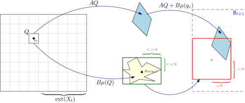
Figure 1: Illustration of the proof of Proposition 1

We begin with the following useful definition.

Definition 11 (Center/Extent of $X\subset\mathbb{R}^{n}$).

Let $X\subset\mathbb{R}^{n}$ be a compact set. Then the center of $X$ is the point $x_{c}\in\mathbb{R}^{n}$ such that for each $i=1,\dots,n$:

$$\llbracket x_{c}\rrbracket_{[i,:]}\triangleq\tfrac{1}{2}\cdot\big{(}\min_{\scriptscriptstyle x\in X}\llbracket x\rrbracket_{[i,:]}+\max_{\scriptscriptstyle x\in X}\llbracket x\rrbracket_{[i,:]}\big{)}$$ (11)

Also, define the extent of $X$ along coordinate $i$ as:

$$\text{ext}_{i}(X)\triangleq\max_{x\in X}\llbracket x-x_{c}\rrbracket_{[i,:]},$$ (12)

and the extent of $X$ as $\text{ext}(X)\triangleq\max_{i=1,\dots,n}\text{ext}_{i}(X)$.

V-A One-Step $\epsilon$ Bounding Box Reachability

Now we can state our second main result: that a one-step bounding box can be computed in polynomial time in the size of a TLL NN controller. We provide two such results, each of which is polynomial in different aspects of the problem.

Theorem 2.

Let $A$, $B$, $X_{t}$ and ${\mathscr{N}\negthickspace\negthickspace\negthinspace\mathscr{N}}\negthinspace\negthinspace\text{{\stixfrak\char 54\relax}}\Xi_{\scriptscriptstyle N,M}^{(m)}\text{{\stixfrak\char 55\relax}}$ be as in the statement of Theorem 1.

Then a one-step $\epsilon=0$ bounding box from $X_{t}$ is computable in time complexity at most (for fixed dimension, $n$):

$$O(m^{n+2}\cdot n^{2}\cdot M\cdot N^{2n+3}\cdot\text{LP}(mN^{2}+N_{X_{t}},n)/n!).$$ (13)

Proof.

This follows almost directly from the proof of Theorem 1. For each of the convex polytopes describing the reachable set, the Fourier-Motzkin elimination can be replaced by $2\cdot n$ LPs to compute its bounding box; these can be combined to determine an $\epsilon=0$ bounding box for $X_{t+1}$ without increasing the complexity noted above. ∎

The result in Theorem 2 certainly meets the criteria of a polynomial-time computation of a one-step bounding box. Unfortunately, the dependence on $N$ and $M$ in Theorem 2 is significant despite being polynomial. However, since we are considering only bounding box reachability, it makes sense to regard the TLL controller as a generic Lipschitz-continuous controller instead: this allows the dependence on its size to be replaced with a dependence on its Lipschitz constant, at the expense of additional (polynomial) dependence on the size of the set $X_{t}$ and the norm of the matrix $B$.

Proposition 1.

Let $A$, $B$, $X_{t}$ and $\mu$ be as in the statement of Definition 7. Furthermore, suppose that $\mu$ is Lipschitz continuous on $X_{t}$, with Lipschitz constant at most $\lVert\mu\rVert$.

Then an $\epsilon$-bounding box from $X_{t}$ is computable in complexity at most (for fixed dimension, $n$):

$$O((2\cdot\text{ext}(X_{t})\cdot\tfrac{2\lVert B\rVert\cdot\lVert\mu\rVert}{\epsilon})^{n}\cdot LP(2\cdot n,n)).$$ (14)

Proof.

$X_{t}$ can be covered by a grid of $(2\cdot\text{ext}(X_{t})\cdot 2\lVert B\rVert\cdot\lVert\mu\rVert/\epsilon)^{n}$ hypercubes whose edges are of width $\epsilon/(2\lVert B\rVert\cdot\lVert\mu\rVert)$. Denote by $Q$ an arbitrary such hypercube, and let $q_{c}$ denote its center. Now observe that for all $q\in Q$:

$$\lVert B\mu(q)-B\mu(q_{c})\lVert\leq\lVert B\rVert\cdot\lVert\mu\rVert\cdot\lVert q-q_{c}\rVert\leq\tfrac{\epsilon}{2}<\epsilon.$$ (15)

Consequently, the set $Q^{\prime}\triangleq\{x:\lVert AQ+B\mu(q_{c})-x\rVert<\epsilon\}$ is guaranteed to be in any $\epsilon$-bounding box of $X_{t+1}$, as is the exact bounding thereof, which we denote by $\text{box}(Q^{\prime})$; see Fig. 1. Clearly $\cup_{Q}\text{box}(Q^{\prime})$ is likewise so contained.

Thus, an $\epsilon$-bounding box from $X_{t}$ can be obtained by examining each $Q$ and computing $\text{box}(Q^{\prime})$. The latter operation entails computing a bounding box for $AQ$, which has the complexity of $LP(2\cdot n,n)$; see Fig. 1. ∎

In particular, for some problems, the quantities in (14) may be much smaller than terms like $N^{2n}$ in (13). In fact, this explains why this type of result is typically not used for NN reachability: it is computationally expensive to compute the exact Lipschitz constant of a generic NN – indeed, it is of exponential complexity in the number of neurons for a deep NN. For a non-degenerate TLL NN, however, it is trivial to compute its exact Lipschitz constant (over all of $\mathbb{R}^{n}$).

Lemma 1.

A bound on the Lipschitz constant of a TLL NN $\Xi_{\scriptscriptstyle N,M}^{(m)}$ over $\mathbb{R}^{n}$ is computable in complexity $O(m\negthinspace\cdot\negthinspace N\negthinspace\cdot\negthinspace n)$. For a non-degenerate TLL (Definition 6), this bound is tight.

Proof.

This is a straightforward application of [6, Proposition 3] or the related result [3, Proposition 4]. The only affine functions realizable by a TLL are those described by its linear layer (see Definition 4). If the TLL is not degenerate, then each of those is realized in its output, hence also lower bounding its Lipschitz constant. The claim follows, since there are $N$ such local linear functions per output, each of whose Lipschitz constants can be computed in $O(n)$. ∎

Theorem 3.

Let $A$, $B$, $X_{t}$ and ${\mathscr{N}\negthickspace\negthickspace\negthinspace\mathscr{N}}\negthinspace\negthinspace\text{{\stixfrak\char 54\relax}}\Xi_{\scriptscriptstyle N,M}^{(m)}\text{{\stixfrak\char 55\relax}}$ be as in the statement of Theorem 1.

Then for any $\epsilon>0$, an $\epsilon$-bounding box from $X_{t}$ can be computed with complexity no more than the maximum of (13) and (14) for $\lVert{\mathscr{N}\negthickspace\negthickspace\negthinspace\mathscr{N}}\negthinspace\negthinspace\text{{\stixfrak\char 54\relax}}\Xi_{\scriptscriptstyle N,M}^{(m)}\text{{\stixfrak\char 55\relax}}\rVert$ bounded according to Lemma 1.

VI The L-TLLBox Algorithm

Theorem 3 establishes a trade-off in computational complexity between two methods for computing an $\epsilon$-bounding box from states $X_{t}$. However, it requires a commitment to the full computational complexity of one algorithm or the other. Moreover, the difference in computational complexity between Theorem 2 and Proposition 1 depends on the characteristics of the TLL controller on the set $X_{t}$ (assuming $\text{ext}(X_{t})$ and $\lVert B\rVert$ are fixed). If the TLL controller has relatively few linear regions intersecting $X_{t}$ but a relatively large Lipschitz constant on $X_{t}$, then Theorem 2 will have lower complexity; recall that Theorem 2 enumerates the linear regions of the TLL controller that intersect $X_{t}$. If, on the other hand, the TLL controller has relatively numerous linear regions intersecting $X_{t}$ but a relatively small Lipschitz constant on $X_{t}$, then Proposition 1 will instead have lower complexity. Thus, the trade off in complexity between Theorem 2 and Proposition 1 amounts to roughly the following: reachability via Proposition 1 is more efficient when the Lipschitz constant of the TLL controller yields a partition of $X_{t}$ into hypercubes (see proof of Proposition 1) each of which “typically” contains many linear regions of the TLL.

This is a salient observation in light of the way that Proposition 1 employs the Lipschitz constant of the TLL controller in question. In Proposition 1, the Lipschitz constant of the TLL controller is really used to create a subdivision of $X_{t}$ into sets such that the output of the TLL controller lies within box of sufficiently small width: see (15). However, note that the Lipschitz constant of a TLL controller over the entire set $X_{t}$ will generally be larger than the Lipschitz constant of the TLL controller on any subset of $X_{t}$. Also, there may be subsets of $X_{t}$ where the TLL controller rapidly switches between large-Lipschitz-constant affine functions such that its output is nevertheless confined to a small box (e.g. a high-frequency saw-tooth function with small amplitude). This suggests the following improvement on Theorem 2 and Proposition 1: identify large subsets of $X_{t}$ where the output of the TLL controller is bounded within a small box – thereby replacing the enumeration of many linear regions of the TLL controller, as in Theorem 2, or the enumeration of many “Lipschitz-width” hypercubes, as in Proposition 1.

Thus, we introduce L-TLLBox as a practical, “adaptive” algorithm, which implements this strategy via the recent tool FastBATLLNN [4]. In particular, FastBATLLNN provides a fast algorithm for obtaining an $\epsilon$-tight bounding box on the output of a TLL controller subject to a convex, polytopic input constraint. This means that FastBATLLNN can be used to directly and efficiently identify subsets of $X_{t}$ where the output of the TLL controller is confined to a small box, without enumerating all of the linear regions of the TLL. That is, for a convex, polytopic set $P\subset X_{t}$ and a box $\mathsf{B}={\sf X}_{i=1}^{m}[l_{i},r_{i}]$ FastBATLLNN can efficiently decide the query:

$$\forall x\in P.{\mathscr{N}\negthickspace\negthickspace\negthinspace\mathscr{N}}\negthinspace\negthinspace\text{{\stixfrak\char 54\relax}}\Xi_{\scriptscriptstyle N,M}^{(m)}\text{{\stixfrak\char 55\relax}}(x)\in\mathsf{B}$$ (16)

by an algorithm that has half the crucial exponent of the algorithms of Theorem 1 and Theorem 2 [6] – i.e., without enumerating the affine regions of the TLL. Thus, for $P$ as above, a tight bounding box on ${\mathscr{N}\negthickspace\negthickspace\negthinspace\mathscr{N}}\negthinspace\negthinspace\text{{\stixfrak\char 54\relax}}\Xi_{\scriptscriptstyle N,M}^{(m)}\text{{\stixfrak\char 55\relax}}(P)$ can be obtained by roughly $\log$ invocations of FastBATLLNN in a binary search on the endpoints of a bounding box.

In this context, the structure of L-TLLBox can be summarized as follows. Start with a hypercube $Q_{1}^{0}$ of edge length $2\cdot\text{ext}(X_{t})$, so that $Q_{1}^{0}$ is large enough to capture the whole set $X_{t}$. Then use FastBATLLNN to determine a sufficiently tight bounding box on the set ${\mathscr{N}\negthickspace\negthickspace\negthinspace\mathscr{N}}\negthinspace\negthinspace\text{{\stixfrak\char 54\relax}}\Xi_{\scriptscriptstyle N,M}^{(m)}\text{{\stixfrak\char 55\relax}}(Q_{1}^{0}\cap X_{t})$. If this bounding box is small enough that its endpoints differ by less than $\epsilon/\lVert B\rVert$ from its center (see (15)), then the reachable bounding box, $\mathsf{B}_{t+1}$ can be updated directly as in Proposition 1. Otherwise, $Q_{1}^{0}$ should be refined into $2^{n}$ hypercubes, each with half its edge lengths, denoted by $Q_{p}^{1}$, $p=1,\dots,2^{n}$, and the process is repeated recursively on each. As above, the recursion stops for a hypercube $Q_{p}^{d}$ at depth $d$ only if FastBATLLNN returns an bounding box for ${\mathscr{N}\negthickspace\negthickspace\negthinspace\mathscr{N}}\negthinspace\negthinspace\text{{\stixfrak\char 54\relax}}\Xi_{\scriptscriptstyle N,M}^{(m)}\text{{\stixfrak\char 55\relax}}(Q_{p}^{d}\cap X_{t})$ whose endpoints are within $\epsilon/\lVert B\rVert$.

This basic recursion is described in Algorithm 1. Three functions in Algorithm 1 require explanation:

• $\mathtt{BBox}(P)$ computes an exact bounding box for the convex polytopic set $P$ using LPs;

• $\mathtt{Subdivide}(Q,p)$ returns the $p^{\text{th}}$ hypercube obtained by splitting each edge of the hypercube $Q$ in half;

• $\mathtt{FastBATLLNN}(\Xi_{\scriptscriptstyle N,M}^{(m)},P,\epsilon)$ returns an $\epsilon$-tight bounding box on the set ${\mathscr{N}\negthickspace\negthickspace\negthinspace\mathscr{N}}\negthinspace\negthinspace\text{{\stixfrak\char 54\relax}}\Xi_{\scriptscriptstyle N,M}^{(m)}\text{{\stixfrak\char 55\relax}}(P)$.

1

2

3

4

5

6

7

input :   $\epsilon>0$

 $A$ an $(n\times n)$ matrix

 $B$ an $(n\times m)$ matrix

 $X_{t}$ a compact, convex polytope of states

 $\Xi_{\scriptscriptstyle N,M}^{(m)}$, parameters of a TLL NN to verify

output :   $\mathtt{B}_{t+1}={\sf X}_{i=1}^{n}[l_{i},r_{i}]$, an $\epsilon$-bounding box from $X_{t}$

8

9global $d\leftarrow 0$

10global $\mathtt{B}_{t+1}\triangleq{\sf X}_{i=1}^{n}[l_{i},r_{i}]\leftarrow{\sf X}_{i=1}^{n}[\infty,-\infty]$

11function LTLLBox($\epsilon$, $A$, $B$, $X_{t}$, $\Xi_{\scriptscriptstyle N,M}^{(m)}$)

12      

13      $d\leftarrow d+1$ // Increment depth counter

14      $Q_{\text{local}}^{d}\leftarrow$ BBox($X_{t}$)

15      for p in $1,\dots,2^{n}$ do

16            

17            // Subdivide $Q_{\text{local}}^{d}$ into $2^{n}$ hypercubes

18            $Q_{p}^{d+1}\leftarrow$ Subdivide($Q_{\text{local}}^{d}$, p)

19            /* Get a bounding box on TLL output to $\epsilon/2$ error for inputs in $Q_{p}^{d+1}\cap X_{t}$ */

20            

21            TLLBx $\leftarrow$ FastBATLLNN($\Xi_{\scriptscriptstyle N,M}^{(m)}$, $Q_{p}^{d+1}\cap X_{t}$, $\tfrac{\epsilon}{2}$)

22            if Width(TLLBx) $<\epsilon/(2\cdot\lVert B\rVert)$ then

23                  

24                  /* Output of TLL is small enough on $Q_{p}^{d+1}$ that we can update $\mathtt{B}_{t+1}$ */

25                  

26                  for i in $1,\dots,n$ do

27                         if Min($\llbracket$BBox($AQ_{p}^{d+1}$)$\rrbracket_{[i,:]}$) - Min($\llbracket$TLLBx $\rrbracket_{[i,:]}$) $<l_{i}$  then

28                              

29                              $l_{i}\leftarrow$ Min($\llbracket$TLLBx $\rrbracket_{[i,:]}$)

30                         end if

31                        if Max($\llbracket$BBox($AQ_{p}^{d+1}$)$\rrbracket_{[i,:]}$) + Max($\llbracket$TLLBx $\rrbracket_{[i,:]}$) $>r_{i}$  then

32                              

33                              $r_{i}\leftarrow$ Max($\llbracket$TLLBx $\rrbracket_{[i,:]}$)

34                         end if

35                        

36                   end for

37                  

38                  return

39             else // Need to refine on $Q_{p}^{d+1}$

40                  

41                  LTLLBox($\epsilon$, $A$, $B$, $Q_{p}^{d+1}\cap X_{t}$, $\Xi_{\scriptscriptstyle N,M}^{(m)}$)

42             end if

43            

44       end for

45      

46 end

Algorithm 1 L-TLL Box core recursion

Formally, we have the following Theorem, which describes the worst-case runtime of L-TLLBox.

Theorem 4.

Let $A$, $B$, $X_{t}$ and ${\mathscr{N}\negthickspace\negthickspace\negthinspace\mathscr{N}}\negthinspace\negthinspace\text{{\stixfrak\char 54\relax}}\Xi_{\scriptscriptstyle N,M}^{(m)}\text{{\stixfrak\char 55\relax}}$ be as in the statement of Theorem 3.

Then for any $\epsilon>0$, L-TLLBox can compute an $\epsilon$ bounding box from $X_{t}$ with a worst-case time complexity of

$$O\Big{(}\log_{2}\big{[}\epsilon\cdot\lVert{\mathscr{N}\negthickspace\negthickspace\negthinspace\mathscr{N}}\negthinspace\negthinspace\text{{\stixfrak\char 54\relax}}\Xi_{\scriptscriptstyle N,M}^{(m)}\text{{\stixfrak\char 55\relax}}\rVert\cdot\text{ext}(X_{t})\cdot\log_{2}\big{[}\tfrac{\text{ext}(X_{t})\cdot\lVert B\rVert\cdot\lVert\mu\rVert}{\epsilon}\big{]}\big{]}\\ m\cdot K\cdot 2^{K\cdot n}\cdot n\cdot M\cdot\tfrac{N^{n+3}}{n!}\cdot\text{LP}(N+N_{X_{t}},n)\Big{)}$$ (17)

where $K=\big{\lceil}\log_{2}\big{(}2\cdot\text{ext}(X_{t})\cdot\tfrac{2\lVert B\rVert\cdot\lVert\mu\rVert}{\epsilon}\big{)}\big{\rceil}$.

Proof.

L-TLLBox recursively subdivides a hypercube of edge length at most $2\cdot\text{ext}(X_{t})$ into $2^{n}$ hypercubes with each recursion. Let $d$ denote the number of recursions, so that at depth $d$, L-TLLBoxhas created at most $2^{d\cdot n}$ hypercubes. Let $Q_{p}^{d}$, $p=1,\dots,2^{d\cdot n}$ denote the hypercubes at depth $d$.

In the worst case, L-TLLBox must recurse on every single hypercube at each depth until all of the resultant subdivided hypercubes have edge length at most $2\cdot\text{ext}(X_{t})\cdot(2\lVert B\rVert\cdot\lVert\mu\rVert)/\epsilon$. This explains the factor $K\cdot 2^{K\cdot n}$: the complexity at each depth is added to the runtime, so the cumulative runtime is dominated by the runtime for the largest recursion depth.

On any given subdivided hypercube, $Q_{p}^{d}$, the complexity of L-TLLBox is dominated by using FastBATLLNN in a binary search on each of the $m$ real-valued TLLs comprising ${\mathscr{N}\negthickspace\negthickspace\negthinspace\mathscr{N}}\negthinspace\negthinspace\text{{\stixfrak\char 54\relax}}\Xi_{\scriptscriptstyle N,M}^{(m)}\text{{\stixfrak\char 55\relax}}$. This is necessary to determine an $\epsilon/2$ bounding box on the output of ${\mathscr{N}\negthickspace\negthickspace\negthinspace\mathscr{N}}\negthinspace\negthinspace\text{{\stixfrak\char 54\relax}}\Xi_{\scriptscriptstyle N,M}^{(m)}\text{{\stixfrak\char 55\relax}}$ when its input is constrained to the set $Q_{p}^{d}$. Since the Lipschitz constant of ${\mathscr{N}\negthickspace\negthickspace\negthinspace\mathscr{N}}\negthinspace\negthinspace\text{{\stixfrak\char 54\relax}}\Xi_{\scriptscriptstyle N,M}^{(m)}\text{{\stixfrak\char 55\relax}}$ is known, the invocations of FastBATLLNN on each output is associated with a binary search over an interval of width $2\cdot\lVert{\mathscr{N}\negthickspace\negthickspace\negthinspace\mathscr{N}}\negthinspace\negthinspace\text{{\stixfrak\char 54\relax}}\Xi_{\scriptscriptstyle N,M}^{(m)}\text{{\stixfrak\char 55\relax}}\rVert\cdot 2\cdot\text{ext}(X_{t})/2^{d}$ until iterations of the search are lie in an interval of width $\epsilon/2$. Thus, each output requires

$$\big{\lceil}\log_{2}\big{(}\epsilon\cdot\lVert{\mathscr{N}\negthickspace\negthickspace\negthinspace\mathscr{N}}\negthinspace\negthinspace\text{{\stixfrak\char 54\relax}}\Xi_{\scriptscriptstyle N,M}^{(m)}\text{{\stixfrak\char 55\relax}}\rVert\cdot\text{ext}(X_{t})/2^{3-d}\big{)}\big{\rceil}$$ (18)

invocations of FastBATLLNN, so the total number of invocations of FastBATLLNN is less than:

$$O\big{(}\log_{2}\big{[}\epsilon\cdot\lVert{\mathscr{N}\negthickspace\negthickspace\negthinspace\mathscr{N}}\negthinspace\negthinspace\text{{\stixfrak\char 54\relax}}\Xi_{\scriptscriptstyle N,M}^{(m)}\text{{\stixfrak\char 55\relax}}\rVert\cdot\text{ext}(X_{t})\cdot\log_{2}\big{[}\tfrac{\text{ext}(X_{t})\cdot\lVert B\rVert\cdot\lVert\mu\rVert}{\epsilon}\big{]}\big{]}\big{)}$$

From [4], each invocation of FastBATLLNN has complexity:

$$n\cdot M\cdot N^{n+3}\cdot\text{LP}(N+N_{X_{t}},n)/n!.$$ (19)

This explains the formula (17). ∎

VII Experiments

To evaluate L-TLLBox as an LTI reachability tool, we used it to perform multi-step bounding box propagation on a number of TLL NN controllers; see Definition 9. We compared the results to NNV’s [12] approximate reachability analysis setting. For this evaluation we selected 40 networks from the TLL Verification Benchmark in the 2022 VNN competition [1]: the first 10 examples from each of the sizes $N=M=8,16,24$ and $32$ were used, and these TLLs were converted to a fully-connected Tensorflow format that NNV could import. Each TLL had $n=2$ inputs and $m=1$ output, so we took these as our state and control dimensions, respectively and generated one random $A$ and $B$ matrix for each TLL NN. We likewise generated one polytopic set of states to serve as $X_{0}$ for each TLL/system combination. Reachability analysis was performed on both tools for $T=3$ discrete time steps. Both tools were given at most 4 days of compute time per TLL/system combination on a standard Microsoft Azure E2ds v5 instance; this instance has one CPU core running at 2.8GHz and 16Gb of RAM and 32Gb swap.

The execution time results of this experiment are summarized by the box-and-whisker plot in Fig. 2. L-TLLBox was able to complete all reachability problems well within the timeout. However, NNV only completed the 10 reachability problems for size $N=8$ and one reachability problem for size $N=16$; it timed out at 4 days for all other problems. On problems where both tools completed the entire reachability analysis, L-TLLBox ranged from 32x faster (the first instance of size $N=8$) to 5,392x faster (the commonly completed instance of $N=16$). For problems that both algorithms finished, the final reachability boxes produced by L-TLLBoxwere anywhere from 0.08 to 1.42 times the area of those produced by NNV. Fig. 3 shows one sequence of reach boxes output by L-TLLBoxand NNV.

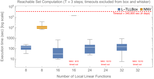
Figure 2: Execution time of L-TLLBox compared to NNV

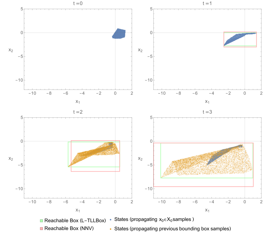
Figure 3: Example reachability box progressions computed by L-TLLBox (25 sec.) and NNV (139,000 sec.); this was the sole $N=16$ reachability sequence completed by NNV.

VIII Conclusions

In this paper, we presented several polynomial complexity results for reachability of an LTI system with a TLL NN controller, including L-TLLBox; these results improve on the exponential complexity for the same reachability problem with a general NN controller, and thus provide a motivation for designing NN controllers using the TLL architecture. As a result, there are a numerous opportunities for future work such as: considering reachability for more general convex sets (e.g. ellipsoidal sets), and generalizing FastBATLLNN so that L-TLLBox can be extended to exact reachability.

References

- [1] VNN competition 2022. https://sites.google.com/view/vnn2022.
- [2] Matthias Althoff, Goran Frehse, and Antoine Girard. Set Propagation Techniques for Reachability Analysis. Annual Review of Control, Robotics, and Autonomous Systems, 4(1), 2021.
- [3] Ulices Santa Cruz, James Ferlez, and Yasser Shoukry. Safe-by-Repair: A Convex Optimization Approach for Repairing Unsafe Two-Level Lattice Neural Network Controllers. In 2022 61st IEEE Conference on Decision and Control (CDC), 2022.
- [4] James Ferlez, Haitham Khedr, and Yasser Shoukry. Fast BATLLNN: Fast Box Analysis of Two-Level Lattice Neural Networks. In Hybrid Systems: Computation and Control 2022 (HSCC’22). ACM, 2022.
- [5] James Ferlez and Yasser Shoukry. AReN: Assured ReLU NN Architecture for Model Predictive Control of LTI Systems. In Hybrid Systems: Computation and Control 2020 (HSCC’20). ACM, 2020.
- [6] James Ferlez and Yasser Shoukry. Bounding the Complexity of Formally Verifying Neural Networks: A Geometric Approach. In 2021 60th IEEE Conference on Decision and Control (CDC), 2021.
- [7] Chao Huang, Jiameng Fan, Xin Chen, Wenchao Li, and Qi Zhu. POLAR: A Polynomial Arithmetic Framework for Verifying Neural-Network Controlled Systems, 2022. http://arxiv.org/abs/2106.13867.
- [8] Radoslav Ivanov, Taylor J. Carpenter, James Weimer, Rajeev Alur, George J. Pappas, and Insup Lee. Verifying the Safety of Autonomous Systems with Neural Network Controllers. ACM Transactions on Embedded Computing Systems, 20(1):7:1–7:26, 2020.
- [9] Guy Katz, Clark Barrett, David L. Dill, Kyle Julian, and Mykel J. Kochenderfer. Reluplex: An Efficient SMT Solver for Verifying Deep Neural Networks. In Computer Aided Verification, Lecture Notes in Computer Science, pages 97–117. Springer International, 2017.
- [10] J. M. Tarela and M. V. Martínez. Region configurations for realizability of lattice Piecewise-Linear models. Mathematical and Computer Modeling, 30(11):17–27, 1999.
- [11] H.-D. Tran, D. Manzanas Lopez, P. Musau, X. Yang, L.-V. Nguyen, W. Xiang, and T. Johnson. Star-Based Reachability Analysis of Deep Neural Networks. In Formal Methods – The Next 30 Years, Lecture Notes in Computer Science. Springer International, 2019.
- [12] Hoang-Dung Tran, Xiaodong Yang, Diego Manzanas Lopez, Patrick Musau, Luan Viet Nguyen, Weiming Xiang, Stanley Bak, and Taylor T. Johnson. NNV: The Neural Network Verification Tool for Deep Neural Networks and Learning-Enabled Cyber-Physical Systems. In Computer Aided Verification, Lecture Notes in Computer Science, pages 3–17. Springer International Publishing, 2020.
- [13] Aladin Virmaux and Kevin Scaman. Lipschitz regularity of deep neural networks: Analysis and efficient estimation. In Advances in Neural Information Processing Systems 31. Curran Associates, 2018.
- [14] Tsui-Wei Weng, Huan Zhang, Hongge Chen, Zhao Song, Cho-Jui Hsieh, Duane Boning, Inderjit S. Dhillon, and Luca Daniel. Towards Fast Computation of Certified Robustness for ReLU Networks, 2018. http://arxiv.org/abs/1804.09699.