A Rogue Planet Helps Populate the Distant Kuiper Belt

Abstract

The orbital distribution of transneptunian objects (TNOs) in the distant Kuiper Belt (with semimajor axes beyond the 2:1 resonance, roughly $a$ = 50–100 au) provides constraints on the dynamical history of the outer solar system. Recent studies show two striking features of this region: 1) a very large population of objects in distant mean-motion resonances with Neptune, and 2) the existence of a substantial detached population (non-resonant objects largely decoupled from Neptune). Neptune migration models are able to implant some resonant and detached objects during the planet migration era, but many fail to match a variety of aspects of the orbital distribution. In this work, we report simulations carried out using an improved version of the GPU-based code GLISSE, following 100,000 test particles per simulation in parallel while handling their planetary close encounters. We demonstrate for the first time that a 2 Earth–mass rogue planet temporarily present during planet formation can abundantly populate both the distant resonances and the detached populations, surprisingly even without planetary migration. We show how weak encounters with the rogue greatly increase the efficiency of filling the resonances, while also dislodging TNOs out of resonance once they reach high perihelia. The rogue’s secular gravitational influence simultaneously generates numerous detached objects observed at all semimajor axes. These results suggest that the early presence of additional planet(s) reproduces the observed TNO orbital structure in the distant Kuiper Belt.

1 Introduction

The heavily studied main Kuiper Belt has semimajor axes smaller than the 2:1 resonance at 48 au (often taken to be the outer boundary of the classical belt). Beyond the 2:1, the transneptunian region seems not as abundantly populated and is dominated by large-eccentricity ($e$) transneptunian objects (TNOs) in the scattering (Trujillo et al., 2000; Lawler et al., 2018b), resonant (Gladman et al., 2012; Crompvoets et al., 2022), and detached (Gladman et al., 2008) populations. This apparent drop in TNO number is partly due to the observational bias that penalizes orbits with large-$a$, large-perihelia ($q$), and large-inclinations ($i$). Deriving the intrinsic TNO orbital distribution at large semimajor axis requires well-characterized surveys that properly handle observation bias. Modern surveys like CFEPS (Petit et al., 2011), OSSOS (Bannister et al., 2018), and DES (Dark Energy Survey; Bernardinelli et al., 2022) all show evidence for an abundant population of $a$ = 50–100 au TNOs (referred to as ‘the distant belt’ here). Studies that accounted for this bias (Gladman et al., 2012; Pike et al., 2015; Volk et al., 2018) all concluded that the distant resonances are heavily populated. The distant $n$:1 resonances are particularly crowded, with populations comparable to the closer 3:2 (Crompvoets et al., 2022). Similar estimates indicate that the detached region hosts at least as many TNOs as the hot classical belt (Petit et al., 2011, Beaudoin et al. 2022, submitted to PSJ). All evidence points to an abundantly populated distant Kuiper Belt whose inventory should be greatly improved by LSST (Collaboration et al., 2009).

Neptune migration models have been proposed to create the distant resonant and detached populations. Hahn & Malhotra (2005) simulated Neptune’s smooth outward migration into both dynamically cold and heated disks; neither case populates the distant resonances as much as the 3:2 and 2:1. Gomes et al. (2008) realized detached objects can be created during Neptune’s migration via Kozai $q$ lifting. Grainy Neptune migrations, in which Neptune’s $a$ jumps due to planet encounters (Nesvorný et al., 2016; Kaib & Sheppard, 2016), are also able to capture some scattering particles into the distant resonances. Pike & Lawler (2017) bias a Nice model simulation from Brasser & Morbidelli (2013) (where Neptune undergoes a high-$e$ phase during outward migration) using the OSSOS survey simulator and conclude this model doesn’t produce large-enough populations for many distant resonances. Crompvoets et al. (2022) suggest their recent resonant-population estimates disfavor all migration models, as they underpopulate the $n$:1 and $n$:2 resonances; instead an underlying sticking of scattering TNOs to the resonances is preferred, although the efficiency is too low (Yu et al., 2018).

Perhaps effects other than migration are important. Passing stars, even in very dense initial stellar birth cluster environment, are ineffective perturbers inside 200 au (Brasser & Schwamb, 2015; Batygin et al., 2020). One way to create high-$q$ TNOs is via the presence of additional mass(es), whose secular gravitational effect elevates objects from the scattering into the detached population. The initial creation and scattering of now-gone planetary-scale objects in the outer solar system is reasonable (egs. Stern, 1991; Chiang et al., 2005; Silsbee & Tremaine, 2018; Gladman & Volk, 2021). Gladman et al. (2002) postulated that additional planetary-mass bodies could account for large-$q$ detached objects like 2000 CR₁₀₅. This evolved into the ‘Rogue Planet’ hypothesis (Gladman & Chan, 2006) in which an Earth-scale Neptune-crossing rogue planet (initially starting on a low eccentricity orbit) temporarily present in the early solar system creates detached TNOs, even as far out as Sedna; they showed that the perihelion-lifting effect is dominated by the single most-massive object, which shares the typical 100-Myr dynamical lifetime of Neptune-scattering bodies. Lykawka & Mukai (2008) also proposed a resident trans-Plutonian planet (with $a=$ 100–175 au, $q>80$ au, and 0.3–0.7 $M_{\oplus}$) to sculpt the Kuiper Belt and generate a substantial population of detached TNOs.

In the context of solar system studies, ‘rogue planets’ refers to planets born in our solar system that are scattered away from their formation location and could have left behind orbital structures caused by their temporary presence. We point out the same terminology is sometimes also applied to interstellar free-floating planets.

In light of the additional high-$q$ TNO discoveries in the last 15 years, we revisit the rogue planet hypothesis. We show that a rogue planet temporarily present on an eccentric orbit sufficiently populates both the resonant and detached populations in the $a$ = 50–100 au Kuiper Belt, even without any planetary migration.

2 Dynamics from the 4 Giant Planets

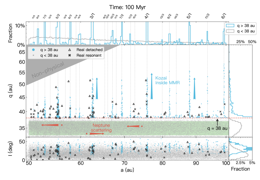
Figure 1: $a,q,i$ distributions of TNOs at 100 Myr in the reference simulation (animated in the online version). The initial conditions have $33<q_{0}<37$ au (shaded green region). Arrows in the $a,q$ panel illustrates the two dominant dynamical effects in the scattering disk: horizontal Neptune scattering (red arrows) and vertical resonant $q$ lifting (blue arrows). The three side panels show histograms for simulated $q<38$ au (gray) and $q>38$ au (blue) particles. At the simulation’s end, only $\simeq$1% of $a$ =  50–100 au particles have $q>38$ au, with the vast majority being resonant objects and almost none being detached objects. The superimposed real $q>38$ au detached objects (black triangles) show an apparent concentration near resonances (especially $n$:1 and $n$:2, labelled at top).

To quantify the dynamical effects in the distant Kuiper Belt induced by the four giant planets alone, we show a reference simulation with a synthetic young scattering disk. 100,000 test particles, starting from $a$=50 au, were placed following a $dN/da\propto a^{-2.5}$ distribution. A uniform $q_{0}$=33–37 au distribution was used to cover the current values of scattering objects, but will allow us to post-facto explore the early scattering disk’s parameters integration by weighting the $q_{0}$ values (Sec. 4). The initial inclination distribution follows $\sin{i}$ times a gaussian of $15^{\circ}$ width, the same distribution as the hot main Kuiper Belt objects (Brown, 2001; Petit et al., 2011). All phase angles ($\Omega$, $\omega$, and $M$) are random and orbital elements are always converted to the J2000 barycentric frame.

We integrated for 100 Myr, with 4 giant planets on their current orbits, using a regularized version of Glisse (Zhang & Gladman, 2022). This modified integrator Glisser can propagate $\sim$10⁵ test particles on a GPU, while resolving close encounters with planets on multiple CPU cores using many Swift subroutine calls (Levison & Duncan, 1994). We have verified this integrator in several common test problems, confirming it correctly handles the resonant dynamics, secular dynamics and scattering dynamics. Glisser provides final orbital distributions statistically identical to those simulated by other standard orbital integrators like Mercury (Chambers, 1999) and Swift (Levison & Duncan, 1994).

The 100 Myr snapshot for the reference simulation’s movie is shown in Fig. 1. We limit our comparisons to $a$ = 50–100 au because this region has a meaningful density of known $q>$ 38 au resonant and detached objects, making a comparison feasible. With four giant planets, two dynamical processes dominate the scattering disk. At $q<$ 38 au, TNOs are steadily scattered due to their proximity at perihelion passages to Neptune’s orbit; this produces horizontal movement (denoted by red particles and arrows in Fig. 1 for a few examples) on the $(a,q)$ plot as scattering TNOs random walk in $a$ while approximately preserving $q$. At larger perihelia, where weaker Neptunian encounters less effectively change the TNO’s orbital elements, the dominant dynamics occurs at Neptunian mean-motion resonances. The resonances allow evolution to higher-$q$ and higher-$i$ orbits via the Kozai-Lidov mechanism inside mean-motion resonances (Kozai, 1962; Gomes et al., 2008). The perihelion evolution (blue dots and arrows in Fig. 1) is clearly stronger along $n$:1 and $n$:2 resonances. Unfortunately, the overall efficiency of the resonant $q$-lifting effect is low, with only $\approx$$1\%$ of $a$ = 50–100 au objects reaching $q>38$ au in 100 Myr. Furthermore, we determined that almost every particle located in Fig. 1’s resonant spikes was initially within $\pm$0.3 au of the corresponding resonant center meaning they by chance started resonant rather than being delivered to it. This indicates that resonant sticking (a mechanism characterized by scattering objects evolving through intermittent temporary resonance captures, Lykawka & Mukai, 2007) is not the main source of the high-$q$ resonant TNOs. We will return to this in Sec. 3.

Compared to real TNOs in the same region (black triangles and crosses in Fig. 1), this reference model produces some resonant objects but barely any detached objects, especially between the resonances at high $q$. This mismatch is unsurprising because Neptune with a largely unchanging orbit is extremely inefficient at detaching objects from the scattering disk (Gladman et al., 2002). Although resonance escape can (rarely) happen at high $q$ without Neptune migration, Gomes et al. (2008, fig. 10) conclude that Neptune migration is needed to break the reversibility. Therefore, grainy migration models (egs. Nesvorný et al., 2016; Kaib & Sheppard, 2016) introduced moderate ($\sim$0.1 au) semimajor axis jumps to Neptune’s migration history in order to detach objects from resonances by suddenly moving the resonance borders. Nesvorný et al. (2016) show how grainy Neptune migration results in greater resonance trapping and although they do not bias their numerical results to see if the orbital distribution matches known TNOs, their detached population agrees with the recent observational measurement (Beaudoin et al. 2022, submitted).

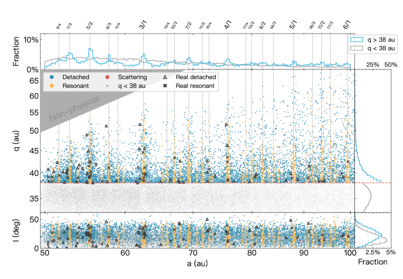
Figure 2: $a,q,i$ distributions and histograms of test particles under 100-Myr gravitational influences of a 2 $M_{\oplus}$ rogue (initial $a_{r}=300$ au, $q_{r}=40$ au, and $i_{r}=20^{\circ}$) and the 4 giant planets. The online animated version shows the entire evolution. Particles are color-coded based on their constantly-evolving dynamical classes when they are above the red dashed line of $q=38$ au. With a rogue present, the resonant population (yellow) is now 3 times larger than in the reference simulation. The detached objects (blue) are created across all semimajor axes, with the high-$q$ ones concentrated near resonances (see the $a$ histogram at the top). Depletions at strong resonances are visible in the $q<38$ au scattering disk (gray), due to the rogue boosting the efficiency of resonant $q$ lifting.

3 Dynamical Effects Induced by the Rogue Planet

The Letter presents a proof of concept that a temporarily present planet (called a rogue) can create high-perihelion objects distributed similarly to the observed Kuiper Belt, with sufficient efficiency to match observations and comparable to grainy migration simulations. We added a $m_{r}=2M_{\oplus}$ rogue with an initial $a_{r}=300$ au, $q_{r}=40$ au, and $i_{r}=20^{\circ}$ orbit to the simulation, and integrated it with the same 100,000 test particles to 100 Myr. The chosen rogue parameters (mass, semimajor axis, and dynamical lifetime) were inspired by the preliminary study of Gladman & Chan (2006) where the authors demonstrated such a rogue detaches objects from the scattering disk through secular $q$ forcing, but they had insufficient statistics to examine the rogue’s role in populating distant resonances and detaching objects from these resonances (which we find is the major dynamical mechanism populating $a$ = 50–100 au). We set the rogue’s $q_{0}$=40 au to produce weak $a_{r}$ mobility over the simulation, as we’re concentrating on the new dynamics the rogue brings to the distant belt, rather than exploring the enormous parameter space of possible rogue histories. The TNO orbital evolution is displayed in Fig. 2.

Each particle in Fig. 2 is categorized into one of three dynamical classifications of detached (blue), resonant (orange), and scattering (red), using its 10-Myr dynamical history (Gladman et al., 2008) around a particular moment in the animated version of Fig. 2. We encourage the reader watch the movie on the journal website, which shows the constantly-evolving dynamical classes of each test particles. Only $q>38$ au particles are color-coded based on these classes; the $q<38$ au particles (gray) are less relevant to the problem we are exploring, as their distribution is largely set by initial conditions.

One striking difference in Fig. 2 is that the rogue’s secular effect detaches TNOs directly from the scattering disk across all semimajor axes. This lifting is faster at larger $a$; for TNOs with $a\ll a_{r}$ and orbital period $P$, the order-of-magnitude $q$ oscillation timescale $P_{\text{sec}}$ induced by the rogue is given by (Gladman & Chan, 2006):

$$\frac{P_{\text{sec}}}{P}\sim\left(\frac{M_{\odot}}{m_{r}}\right)\left(\frac{a_{r}}{a}\right)^{3}\left(1-e_{r}^{2}\right)^{3/2},$$ (1)

where $e_{r}$ is the rogue’s eccentricity. For a 2 $M_{\oplus}$ rogue with $a_{r}\simeq 300$ au and $e_{r}\simeq 0.87$, $P_{\text{sec}}$ for $a=50$–100 au varies from $\simeq$1.5 Gyr to 500 Myr, longer than the $\sim$100 Myr dynamical lifetime of the rogue.

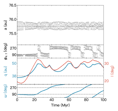
(a) No rogue

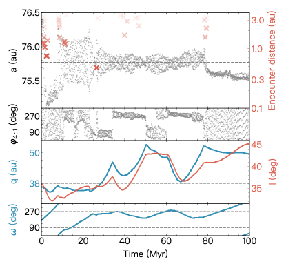
(b) With rogue

Figure 3: Dynamical evolutions of two particles initially near the 4:1 resonance from the reference simulation (left) and the rogue planet simulation (right). From top to bottom, the left axes of both plots are semimajor axis ($a$), the 4:1 resonant angle ($\varphi_{\text{4:1}}$), perihelion ($q$), and argument of perihelion ($\omega$). The right axes are proximity of rogue encounters (denoted by red ‘x’s) and inclination ($I$). Without the rogue present, the Kozai mechanism (represented by $\omega$ librating around $90^{\circ}$ or $270^{\circ}$) is able to raise resonant particle’s perihelion, but spontaneous decoupling from the resonance is highly unlikely. In comparison, the rogue helps build the detached population by both pushing the particle into the resonance and kicking it out at high $q$.

We detail a previously unreported dynamical effect that creates detached TNOs through a combination of Neptunian resonances and rogue encounters. We observe that weak encounters with the rogue are continuously nudging TNOs in semimajor axes, sometimes randomly pushing them into a nearby resonance from the scattering disk. Similarly, rogue encounters are capable of kicking objects out of the resonance; if this happens to occur at high perihelion after part of a Kozai cycle, it naturally forms detached objects near resonances, especially near those with strong $q$ lifting effectiveness like $n$:1 and $n$:2. Both the resonant ‘pushing in’ and ‘kicking out’ happen; our simulation shows the net effect is a $3\times$ enhancement to the resonant population (compared to Fig. 1’s reference simulation), in addition to the considerable quantity of detached TNOs formed around resonances. The power of the rogue-aided $q$ lifting is visible in the deficits of scattering objects (gray dots and upper histogram in Fig. 2) at the resonant semimajor axes. Detached objects with $a<80$ au and $q>40$ au seem to concentrate near resonances, as do real detached TNOs (the movie illustrates these dynamics clearly). The resonance works as a sort of ‘water fountain’, constantly pumping the particles to higher $q$; meanwhile the rogue supplies particles from the scattering disk, and ‘splashes’ them to nearby detached states along the resonances. Such fountain-like structures with a central resonant population and surrounding detached population are visible near strong resonances like 5:2, 3:1, and 4:1.

We selected a particle near the 4:1 from each of the two simulations and plot their evolutions (Fig. 3). The reference simulation’s particle (Fig. 3a) is initially inside the 4:1 resonance. It demonstrates a (rare) $\sim$25 Myr Kozai cycle, enabled by $\omega$ remaining near $90^{\circ}$ initially and diagnosed by strong $e$ and $i$ coupling; this lifts $q$ from 37 au to 50 au and $i$ from $20^{\circ}$ to above $30^{\circ}$. Once Kozai stops ($\omega$ circulates), the still-resonant particle’s critical angle jumps back and forth chaotically between the two asymmetrical libration centers (Morbidelli et al., 1995), with $q$ and $i$ remaining high. However, without additional disturbance (from a jumping Neptune or external rogue), it is almost impossible to spontaneously decouple from the resonance and thus become detached.

Fig. 3b shows a case from the rogue scenario, but here the TNO is initially near but not inside the 4:1 resonance. Each red cross (top panel) marks a time and encounter distance with the rogue. These encounters nudge the particle’s $a$, thus changing its resonant dynamical behaviour. At $\approx$10 Myr, weak encounters move the particle into the 4:1, beginning $\varphi$ libration around $\sim$270^∘. Interestingly, little $q$ and $i$ evolution occurs until a deep encounter pushes the TNO into a part of the resonant parameter space where Kozai activates. After several $q$ and $i$ oscillations from 25–80 Myr, additional encounters at $\approx$2 au distance kick the object out of the resonance, leaving $q\approx 50$ au and $i\approx 45^{\circ}$, creating a detached TNO near the resonant border.

The juxtaposition of Fig. 3’s two plots shows three dynamical effects the rogue induces via encounters: (1) randomly pushing nearby non-resonant scattering disk objects into the resonance, (2) boosting the $q$ lifting by supplying resonant particles into the parameter space where the Kozai cycle operates, and (3) randomly kicking resonant particles out and forming part of the detached population if this occurs at high perihelion.

Only a small faction of the $N$ scattering objects (that intersect rogue’s orbit and are near the mutual node) will be affected per rogue orbit. Over the rogue’s lifetime the entire scattering disk can have rogue encounters because of mutual precession of the rogue and TNO orbit. One can analytically estimate the accumulated encounter number $N_{\text{enc}}$ closer than $\beta$ Hill spheres as

$$\dfrac{N_{\text{enc}}}{N}\simeq 6\;\beta^{2}\left(\dfrac{T_{r}}{100\ \text{Myr}}\right)\left(\dfrac{m_{r}}{2M_{\oplus}}\right)^{\frac{2}{3}}\left(\dfrac{a_{r}}{300\ \text{au}}\right)^{-\frac{3}{2}},$$ (2)

where $N$ is the number of TNOs between the rogue perihelion and aphelion, and $T_{r}$ is the rogue’s dynamical lifetime. For our simulations, the numerical integrator logged the $\beta<1$ encounters, recording $\approx$5 encounters per particle in 100 Myr, in excellent agreement.

Each encounter perturbs different TNO orbital elements; we focus on the rogue’s effect on semimajor axes, as the random nudges in $a$ are what determine resonance entrance and exit. We estimate $|\Delta a|$ for a typical rogue encounter at $\beta R_{H}$ flyby distance as:

$$|\Delta a|\simeq\dfrac{0.1\ \text{au}}{\beta}\left(\dfrac{m_{r}}{2M_{\oplus}}\right)^{\frac{2}{3}}\left(\dfrac{a}{50\ \text{au}}\right).$$ (3)

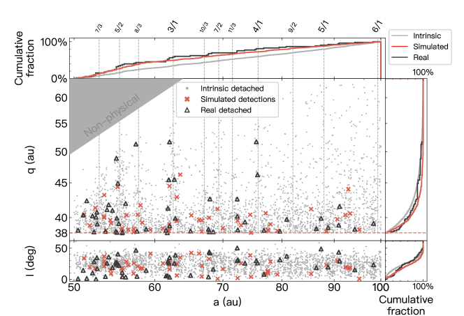
Figure 4: $a,q,i$ distributions of the detached (gray dots), the simulated detections (red crosses), and the real $q>38$ au detached objects (black triangles). The intrinsic sample is built by the rogue and has been eroded to 4 Gyr (only particles with initial $q_{0}<35$ au are included in this plot), on the basis of which the simulated detections are drawn using the OSSOS survey simulator. A decent correspondence between the simulated and the red detached can be found on the three cumulative histograms; a valid proof that the rogue is capable of creating the observed TNO distributions.

For $a$ = 50–100 au, encounters at 1 $R_{H}$ induce $\Delta a\simeq 0.1$–0.2 au for the TNO, approaching the $\simeq\pm$0.5 au width of the nearby resonances (Lan & Malhotra, 2019). This allows encounters to knock TNOs in and out of resonance or shift them inside the resonance, allowing activation of Kozai cycling. Deeper encounters inducing larger $\Delta a$ do exist (Fig. 3b), but Eq. (2) shows encounters become quadratically rarer with decreasing $\beta$. An average TNO suffers a passage no closer than 0.4$R_{H}$ for Fig. 2’s rogue.

These encounters greatly increase how many TNOs end up in the high-$q$ region. We find the rogue’s 100 Myr presence raises 10% of the $a$=50–100 au scattering disk objects to $q>38$ au, with 3% being resonant and 7% being detached. Compared to the reference simulation, this rogue scenario emplaces an order of magnitude more TNOs in the high-$q$ region. We also did a preliminary exploration of varying the rogue’s mass; two additional 100 Myr simulations show that 0.5 $M_{\oplus}$ or 1 $M_{\oplus}$ rogues still populate the high-$q$ region, but with lower efficiency (with 3.3% and 5.5%, respectively, of TNOs having $q>38$ au). Both the rogue’s time $T_{r}$ intersecting the belt and its $a_{r}$ and $e_{r}$ evolution history (Eqs. 1 and 2) influences its sculpting of the distant Kuiper Belt’s structure.

4 Estimating Observation Bias

The real TNOs in Fig. 2 are more concentrated to low-$a$ and low-$q$ than the distribution produced by the rogue. This is expected given observational bias which favors them. Observation biases differ from survey to survey, but the first-order effect for near-ecliptic surveys is that it penalizes large-$a$, large-$q$, and large-$i$ orbits.

To verify whether our numerically simulated TNO distribution is similar to the observed Kuiper Belt, we forward bias the numerical sample to compare it with the real objects. Lawler et al. (2018a) details how this forward biasing is done using a ‘survey simulator’. Biases for resonant objects are complex to simulate, as their perihelion passages are correlated to Neptune’s location, resulting in detection preferentially at specific longitudes relative to Neptune (Gladman et al., 2012). Lacking detailed pointing information for many past surveys, we do not compare to the resonant objects, instead focusing on $q>38$ au detached TNOs.

We first eroded the surviving test particles for 4 Gyr with only the four giant planets. That is, the rogue was assumed to be ejected after a typical dynamical lifetime of 100 Myr; in this case we manually removed it before the 4 Gyr integration. The dynamical classification algorithm was then repeated to remove resonant and scattering TNOs from the $q>38$ au sample, and the remaining detached TNOs are plotted in Fig. 4 (gray dots). The uniform initial $q_{0}$ distribution allowed us to weight the sample post-facto and we found obvious improvement in the match keeping only $q_{0}<35$ au (see below). We superpose 53 real detached objects (black triangles); these TNOs were identified by Gladman & Volk (2021), consisting of the OSSOS detached (Bannister et al., 2018) and other TNOs with sufficiently good orbits. We utilized the OSSOS survey simulator to generate 689 simulated detections; a random 53 of them (the same as the real sample) are plotted (red crosses) to illustrate the biases. Cumulative $a$, $q$, and $i$ histograms for $\sim$2800 intrinsic (model) particles, the 689 simulated detections, and the 53 real objects are on Fig. 4’s side panels. Because detached TNOs from other surveys do not share the same detection biases as OSSOS, this preliminary comparison is only approximate.

Fig. 4’s cumulative distributions exhibit (perhaps surprisingly) good agreement between the simulated detections (red) and the real detached objects (black). When using all numerical initial conditions, the simulated $a$ and $q$ distributions have the general trend of the real detections, but restricting to $q_{0}<35$ au produces an obvious improvement. We take this as evidence that much of the perihelion lifting began at an early stage when the scattering disk was still developing; Fig. 3 of Gladman (2005) shows that in the first 50 Myr only $q<35$ au orbits are populated, only after $\sim$1 Gyr do scattering TNOs extend up to $q=37$. The superiority of a more confined $q_{0}$ distribution is verified in Beaudoin et al. (2022, submitted to PSJ), who more rigorously compares with only the OSSOS objects; they show that the $q_{0}<35$ au detached TNO $q$ distribution created by the 2-$M_{\oplus}$ rogue is non-rejectable, with Anderson-Darling probability of $32\%$ (and is in fact the best model they studied).

5 Discussion

We demonstrate for the first time that a rogue planet present for $\sim$100 Myr during planet formation can abundantly create both the distant resonant and detached populations. This is accomplished by the synergy of the Neptunian resonances (with the Kozai mechanism lifting perihelia) and weak rogue encounters (where the rogue supplies the resonance and detaches objects at high $q$). Several points merit discussion.

The Cold Classical Belt. A potential concern regarding the temporary presence of Earth-scale planets is the possibility of dynamically heating the cold classical belt, which is often thought to be formed in-situ and unexcited for the age of the solar system. The observed limits on the $e$ and $i$ excitation are used to constrain Neptune’s dynamical history (Batygin et al., 2011; Dawson & Murray-Clay, 2012; Nesvorný & Vokrouhlický, 2016), including the absence of planets formed in the cold belt itself (Morbidelli et al., 2002). A rogue must have scattered to large $a$ early, as even a few million-year residence with $a_{r}\simeq$ 50 au would excite the cold belt. Once the rogue reaches $a$ of a few hundred au, the average time it stays in the classical belt drops by $a^{3/2}$ (Eq. 2), greatly reducing the cold-belt’s excitation. We confirmed this with simple numerical simulation of just the cold classical belt, placing 10,000 objects with initial $e_{0}=10^{-3}$ and $i_{\text{free}}<0.2^{\circ}$ (Huang et al., 2022) from $a_{0}=42$ au to 47 au and integrated with the same rogue in Sec. 3. Even though the rogue continuously crosses this cold belt for 100 Myr, its gravity induces surprisingly little excitation: the vast majority of cold TNOs keep $e<0.05$ and $i_{\text{free}}<1^{\circ}$ (Fig. 5). We conclude a large-$a$ rogue does not unacceptably excite the cold belt.

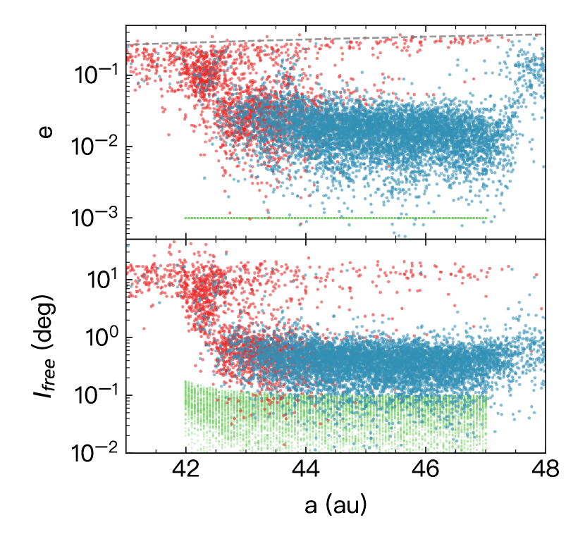
Figure 5: Orbital excitation of the cold classical Kuiper Belt, after 100 Myr of perturbation from the rogue with $a,q,i$ of roughly 300 au, 40 au, and 20^∘. Green points mark initial conditions, and red/blue points show final values for particles that began with $a_{0}$ smaller/larger than 43 au, respectively. From initial $e_{0}=10^{-3}$ and $i_{\text{free}}<0.2^{\circ}$, the surviving cold main belt with $a_{0}>43$ au remains with low $e$ and $i$. For $a_{0}<43$ au secular resonances ($g_{8}$ and $s_{8}$) pump both $e$ and $i$ after which particles scatter to all values of $a$ along the Neptune crossing line (gray dashed). Repeating the simulation using Rebound (Rein & Liu, 2012) produces the same excitations. Thus, the rogue does not unacceptably excite the cold belt, whose TNOs currently have even higher values of $e$ and $i$.

Oort Cloud Building. The period of the rogue’s existence will coincide with the epoch in which the Oort cloud is created (Duncan et al., 1987; Dones et al., 2004; Portegies Zwart et al., 2021). Although in principle one might worry that an Earth-scale rogue at 100 au could strongly interfere with the creation of the Oort cloud, Lawler et al. (2017) show that the presence of even a larger 10 $M_{\oplus}$ object in the 250–750 au range for the entire age of the Solar System lowers Oort cloud implantation efficiency by only a factor of $\simeq$2. The efficiency of Oort cloud implantation and its mass are sufficiently uncertain (Portegies Zwart et al., 2021) that there is no obvious problem with the temporary presence of a rogue like we envision.

Sun’s Birth Environment. The rogue’s highly-eccentric orbit of a few hundred au could be affected by close-in stellar flybys that could have happened in the Sun’s birth environment. Arguments have been made that our Sun was likely born in a cluster of 1000-3000 stars/pc³, based on extinct radionuclides and the assumption that extreme detached TNOs, represented by Sedna, needed to produced in the birth cluster environment (Portegies Zwart, 2009; Adams, 2010; Pfalzner, 2013). The question is how quickly the Sun exited this birth cluster. If Sun remained for a long time, there would be problems with retaining the Oort cloud (egs. Morbidelli & Levison, 2004; Nordlander et al., 2017). In addition, the recent study by Batygin et al. (2020) computes an upper bound of number density-weighted cluster residence of our Sun of $2\times 10^{4}$ Myr/pc³, based on the unexcited inclination distribution of the cold classical belt; this implies that the Sun must have exited its birth cluster in less than $\sim$15 Myr, using their 1400 stars/pc³ estimate (Batygin & Brown, 2021). Similar early exit arguments are given by Brasser et al. (2006) and Pfalzner (2013), both of which suggest 5 Myr residence. The timescale for the rogue to reach several hundred au is comparable to this $\sim$10 Myr duration and we therefore think a 100 Myr survival timescale for the rogue is not problematic. Furthermore, the rogue’s presence directly provides a way other than the Sun’s birth cluster to explain Sednoids (Gladman & Chan, 2006), which would alleviate the “need to make Sedna with passing stars” constraint (fig. 7 of Adams, 2010; Pfalzner, 2013; Brasser & Schwamb, 2015) in the Sun’s birth environment.

An Existing Planet. The natural 100 Myr ejection time scale for scattering rogues (Gladman & Chan, 2006) sets a typical time scale that we have seen produces the needed detached and resonant populations in the 50–100 au region. Instead of ejection, if the rogue’s perihelion was lifted (by an unspecified process) to very large $q$, it could remain in the outer solar system today and negligibly affect the 50-100 au region. Scenarios with a still-resident rogue (Sheppard & Trujillo, 2016; Batygin et al., 2019) presumably began with that planet on low-$q$ orbit for some period; that combination of $T_{r}$, $m_{r}$, and $a_{r}$ (Eq. 2) while $q_{r}<100$ au could produce the same effects we study, before the mysterious $q_{r}$ lift. But given that recent surveys (Shankman et al., 2017; Napier et al., 2021; Bernardinelli et al., 2022) do not support intrinsic clustering, we find the ‘now gone’ rogue scenario to be more natural.

Neptune Migration. It is generally believed that Neptune migrated outwards during the planet-formation and disk-dispersal epoch (reviewed by Nesvorný, 2018). The ‘grainy’ migration models (see Sec. 2) are effective at creating detached TNOs when Neptune’s semimajor axis jumps (and thus so do all its resonances) due to encounters with dwarf planets; if the jumps become comparable to the resonance size ($>$0.1 au, say), then some particles are suddenly no longer in resonance. A final phase of slow net-outward grainy migration results in an asymmetry of ‘stranded’ particles on the sunward side of the resonance (Kaib & Sheppard, 2016; Nesvorný et al., 2016). There is growing observational evidence for this (Lawler et al., 2019; Bernardinelli et al., 2022); after fixing an error in the Dark Energy Survey selection function (working with Bernardinelli, private communication 2022), we combined the $q>38$ au samples from these two studies and find that the binomial probability that the detached number just beyond each resonance is comparable to those on the sunward side remains $<$1%.

Regarding detachment, we find the rogue planet scenario produces comparable numbers of detached TNOs. This is not too surprising, if one takes the view that the rogue produces ‘grainy’ TNO jumps while grainy migration jumps the resonances. In our case, Eq. (3)’s $\Delta a$ is set by the range of encounter distances and the rogue’s mass, while in grainy migration models there is an assumed mass spectrum of the bodies encountering Neptune (at a range of flyby distances). It is likely that after the rogue’s ejection there will still be moderately-massive scattering disk; during its erosion a final small outward Neptune migration will then occur. This would capture stranded TNOs on the high-$a$ side of the resonance and continue ‘littering’ TNOs on the sunward side, giving an outcome very similar to migration alone.

A unique outcome of our study is that we have rigorously compared the simulation’s final orbital distribution to the known OSSOS TNOs, and find excellent agreement (Beaudoin et al. 2022, submitted to PSJ), yielding a population estimate of 40,000 detached TNOs with diameters $>$100 km, a number identical to the Nesvorný et al. (2016) population estimate, who didn’t have the information necessary for rigorous orbital comparison. Additionally, having a rogue during this period simultaneously allows the production of large-$q$ objects like Sedna (Gladman & Chan, 2006).

We believe that both processes operated in our early Solar System because it is natural that objects between Pluto and ice-giant scale existed during disk dispersal. The rogue’s presence introduces another mechanism to produce many features seen in the distant Kuiper Belt. We believe that rogues and migration are both expected outcomes of the process of planet building; the uncertainties introduced into deriving parameters (such as the migration duration and mass spectrum of other bodies in the system) in future models which incorporate both seem unavoidable.

6 Acknowledgements

We thank F. Adams, P. Bernardinelli, L. Dones, , S. Lawler, S. Tremaine, K. Volk, and an anonymous referee for useful discussions. YH acknowledges support from China Scholarship Council (grant 201906210046) and the Edwin S.H. Leong International leadership fund, BG acknowledges Canadian funding support from NSERC.

References

- Adams (2010) Adams, F. C. 2010, ARA&A, 48, 47, doi: 10.1146/annurev-astro-081309-130830
- Bannister et al. (2018) Bannister, M. T., Gladman, B. J., Kavelaars, J. J., et al. 2018, ApJS, 236, 18, doi: 10.3847/1538-4365/aab77a
- Batygin et al. (2020) Batygin, K., Adams, F. C., Batygin, Y. K., & Petigura, E. A. 2020, AJ, 159, 101, doi: 10.3847/1538-3881/ab665d
- Batygin et al. (2019) Batygin, K., Adams, F. C., Brown, M. E., & Becker, J. C. 2019, Phys. Rep., 1 , doi: 10.1016/j.physrep.2019.01.009
- Batygin & Brown (2021) Batygin, K., & Brown, M. E. 2021, ApJ, 910, L20, doi: 10.3847/2041-8213/abee1f
- Batygin et al. (2011) Batygin, K., Brown, M. E., & Fraser, W. C. 2011, ApJ, 738, 13, doi: 10.1088/0004-637x/738/1/13
- Bernardinelli et al. (2022) Bernardinelli, P. H., Bernstein, G. M., Sako, M., et al. 2022, ApJS, 258, 41, doi: 10.3847/1538-4365/ac3914
- Brasser et al. (2006) Brasser, R., Duncan, M., & Levison, H. 2006, Icarus, 184, 59, doi: 10.1016/j.icarus.2006.04.010
- Brasser & Morbidelli (2013) Brasser, R., & Morbidelli, A. 2013, Icarus, 225, 40, doi: 10.1016/j.icarus.2013.03.012
- Brasser & Schwamb (2015) Brasser, R., & Schwamb, M. E. 2015, MNRAS, 446, 3788, doi: 10.1093/mnras/stu2374
- Brown (2001) Brown, M. E. 2001, AJ, 121, 2804, doi: 10.1086/320391
- Chambers (1999) Chambers, J. E. 1999, MNRAS, 304, 793, doi: 10.1046/j.1365-8711.1999.02379.x
- Chiang et al. (2005) Chiang, E., Lithwick, Y., Murray-Clay, R., et al. 2005, A Brief History of Transneptunian Space, ed. B. Reipurth & D. Jewitt, Protostars and Planets V (Tucson: University of Arizona Press)
- Collaboration et al. (2009) Collaboration, T. L. S. S. S., Jones, R. L., Chesley, S. R., et al. 2009, Earth, Moon, and Planets, 105, 101, doi: 10.1007/s11038-009-9305-z
- Crompvoets et al. (2022) Crompvoets, B. L., Lawler, S. M., Volk, K., et al. 2022, \psj, 3, 113, doi: 10.3847/psj/ac67e0
- Dawson & Murray-Clay (2012) Dawson, R. I., & Murray-Clay, R. 2012, ApJ, 750, 43, doi: 10.1088/0004-637x/750/1/43
- Dones et al. (2004) Dones, L., Weissman, P., Levison, H., & Duncan, M. 2004, Oort Cloud Formation and Dynamics, ed. M. C. Festou, H. U. Keller, & H. A. Weaver, Comet II (Tucson: University of Arizona Press)
- Duncan et al. (1987) Duncan, M., Quinn, T., & Tremaine, S. 1987, AJ, 94, 1330, doi: 10.1086/114571
- Gladman (2005) Gladman, B. 2005, Science, 307, 71, doi: 10.1126/science.1100553
- Gladman & Chan (2006) Gladman, B., & Chan, C. 2006, ApJ, 643, L135 , doi: 10.1086/505214
- Gladman et al. (2002) Gladman, B., Holman, M., Grav, T., et al. 2002, Icarus, 157, 269, doi: 10.1006/icar.2002.6860
- Gladman et al. (2008) Gladman, B., Marsden, B. G., & Vanlaerhoven, C. 2008, The Solar System Beyond Neptune, Vol. 43, Nomenclature in the Outer Solar System, ed. M. A. Barucci, H. Boehnhardt, D. P. Cruikshank, & A. Morbidelli (Tucson: University of Arizona Press)
- Gladman & Volk (2021) Gladman, B., & Volk, K. 2021, ARA&A, 59, 203, doi: 10.1146/annurev-astro-120920-010005
- Gladman et al. (2012) Gladman, B., Lawler, S. M., Petit, J. M., et al. 2012, AJ, 144, 23, doi: 10.1088/0004-6256/144/1/23
- Gomes et al. (2008) Gomes, R. S., Fernández, J. A., Gallardo, T., & Brunini, A. 2008, The Scattered Disk: Origins, Dynamics, and End States, ed. M. A. Barucci, H. Boehnhardt, D. P. Cruikshank, & A. Morbidelli, The Solar System Beyond Neptune (Tucson: University of Arizona Press). https://ui.adsabs.harvard.edu/abs/2008ssbn.book..259G/abstract
- Hahn & Malhotra (2005) Hahn, J. M., & Malhotra, R. 2005, AJ, 130, 2392, doi: 10.1086/452638
- Huang et al. (2022) Huang, Y., Gladman, B., & Volk, K. 2022, ApJS, 259, 54, doi: 10.3847/1538-4365/ac559a
- Kaib & Sheppard (2016) Kaib, N. A., & Sheppard, S. S. 2016, AJ, 152, 133, doi: 10.3847/0004-6256/152/5/133
- Kozai (1962) Kozai, Y. 1962, AJ, 67, 579, doi: 10.1086/108876
- Lan & Malhotra (2019) Lan, L., & Malhotra, R. 2019, Celestial Mechanics and Dynamical Astronomy, 131, 39, doi: 10.1007/s10569-019-9917-1
- Lawler et al. (2018a) Lawler, S. M., Kavelaars, J. J., Alexandersen, M., et al. 2018a, Frontiers in Astronomy and Space Sciences, 5, 14, doi: 10.3389/fspas.2018.00014
- Lawler et al. (2017) Lawler, S. M., Shankman, C., Kaib, N., et al. 2017, AJ, 153, 33, doi: 10.3847/1538-3881/153/1/33
- Lawler et al. (2018b) Lawler, S. M., Shankman, C., Kavelaars, J. J., et al. 2018b, AJ, 155, 197, doi: 10.3847/1538-3881/aab8ff
- Lawler et al. (2019) Lawler, S. M., Pike, R. E., Kaib, N., et al. 2019, AJ, 157, 253, doi: 10.3847/1538-3881/ab1c4c
- Levison & Duncan (1994) Levison, H. F., & Duncan, M. J. 1994, Icarus, 108, 18 , doi: 10.1006/icar.1994.1039
- Levison & Duncan (1997) —. 1997, Icarus, 127, 13, doi: 10.1006/icar.1996.5637
- Lykawka & Mukai (2007) Lykawka, P. S., & Mukai, T. 2007, Icarus, 192, 238, doi: 10.1016/j.icarus.2007.06.007
- Lykawka & Mukai (2008) —. 2008, AJ, 135, 1161, doi: 10.1088/0004-6256/135/4/1161
- Morbidelli et al. (2002) Morbidelli, A., Jacob, C., & Petit, J.-M. 2002, Icarus, 157, 241, doi: 10.1006/icar.2002.6832
- Morbidelli & Levison (2004) Morbidelli, A., & Levison, H. F. 2004, AJ, 128, 2564, doi: 10.1086/424617
- Morbidelli et al. (1995) Morbidelli, A., Thomas, F., & Moons, M. 1995, Icarus, 118, 322 , doi: 10.1006/icar.1995.1194
- Napier et al. (2021) Napier, K. J., Gerdes, D. W., Lin, H. W., et al. 2021, \psj, 2, 59, doi: 10.3847/psj/abe53e
- Nesvorný (2018) Nesvorný, D. 2018, ARA&A, 56, 137 , doi: 10.1146/annurev-astro-081817-052028
- Nesvorný & Vokrouhlický (2016) Nesvorný, D., & Vokrouhlický, D. 2016, ApJ, 825, 94, doi: 10.3847/0004-637x/825/2/94
- Nesvorný et al. (2016) Nesvorný, D., Vokrouhlický, D., & Roig, F. 2016, ApJ, 827, L35, doi: 10.3847/2041-8205/827/2/l35
- Nordlander et al. (2017) Nordlander, T., Rickman, H., & Gustafsson, B. 2017, A&A, 603, A112, doi: 10.1051/0004-6361/201630342
- Petit et al. (2011) Petit, J. M., Kavelaars, J. J., Gladman, B. J., et al. 2011, AJ, 142, 131, doi: 10.1088/0004-6256/142/4/131
- Pfalzner (2013) Pfalzner, S. 2013, A&A, 549, A82, doi: 10.1051/0004-6361/201218792
- Pike et al. (2015) Pike, R. E., Kavelaars, J. J., Petit, J. M., et al. 2015, AJ, 149, 202, doi: 10.1088/0004-6256/149/6/202
- Pike & Lawler (2017) Pike, R. E., & Lawler, S. M. 2017, AJ, 154, 171, doi: 10.3847/1538-3881/aa8b65
- Portegies Zwart et al. (2021) Portegies Zwart, S., Torres, S., Cai, M. X., & Brown, A. G. A. 2021, A&A, 652, A144, doi: 10.1051/0004-6361/202040096
- Portegies Zwart (2009) Portegies Zwart, S. F. 2009, ApJ, 696, L13, doi: 10.1088/0004-637x/696/1/l13
- Rein & Liu (2012) Rein, H., & Liu, S.-F. 2012, A&A, 537, A128, doi: 10.1051/0004-6361/201118085
- Shankman et al. (2017) Shankman, C., Kavelaars, J. J., Bannister, M. T., et al. 2017, AJ, 154, 50, doi: 10.3847/1538-3881/aa7aed
- Sheppard & Trujillo (2016) Sheppard, S. S., & Trujillo, C. 2016, AJ, 152, 221, doi: 10.3847/1538-3881/152/6/221
- Silsbee & Tremaine (2018) Silsbee, K., & Tremaine, S. 2018, AJ, 155, 75, doi: 10.3847/1538-3881/aaa19b
- Stern (1991) Stern, S. 1991, Icarus, 90, 271, doi: 10.1016/0019-1035(91)90106-4
- Trujillo et al. (2000) Trujillo, C. A., Jewitt, D. C., & Luu, J. X. 2000, ApJ, 529, L103, doi: 10.1086/312467
- Volk et al. (2018) Volk, K., Murray-Clay, R. A., Gladman, B. J., et al. 2018, AJ, 155, 260 , doi: 10.3847/1538-3881/aac268
- Yabushita (1980) Yabushita, S. 1980, A&A
- Yu et al. (2018) Yu, T. Y. M., Murray-Clay, R., & Volk, K. 2018, AJ, 156, 33, doi: 10.3847/1538-3881/aac6cd
- Zhang & Gladman (2022) Zhang, K., & Gladman, B. J. 2022, New Astronomy, 90, 101659, doi: 10.1016/j.newast.2021.101659