Generative Graphical Inverse Kinematics
Abstract
Quickly and reliably finding accurate inverse kinematics (IK) solutions remains a challenging problem for robotic manipulation. Existing numerical solvers are broadly applicable, but typically only produce a single solution and rely on local search techniques to minimize highly nonconvex objective functions. More recent learning-based approaches that approximate the entire feasible set of solutions have shown promise as a means to generate multiple fast and accurate IK results in parallel. However, existing learning-based techniques have a significant drawback: each robot of interest requires a specialized model that must be trained from scratch. To address this key shortcoming, we investigate a novel distance-geometric robot representation coupled with a graph structure that allows us to leverage the flexibility of graph neural networks (GNNs). We use this approach to train the first learned generative graphical inverse kinematics (GGIK) solver that is able to produce a large number of diverse solutions in parallel and to also generalize: a single learned model can be used to produce IK solutions for a variety of different robots. When compared to several other learned IK methods, GGIK provides more accurate solutions. GGIK is also able to generalize reasonably well to robot manipulators unseen during training. Finally, we show that GGIK can be used to complement local IK solvers by providing reliable initializations to seed the local optimization process.
I Introduction
Robotic manipulation tasks are naturally defined in terms of end-effector positions and poses (e.g., for bin-picking or path following). However, the configuration of a manipulator is typically specified in terms of joint angles, and determining the joint configuration(s) that correspond to a given end-effector pose requires solving the inverse kinematics (IK) problem. For redundant manipulators (i.e., those with more than six degrees of freedom or DOF), target poses may be reachable by an infinite set of feasible configurations. While redundancy allows high-level algorithms (e.g., motion planners) to choose configurations that best fit the overall task, it makes solving IK substantially more involved.
Since the full set of IK solutions cannot, in general, be derived analytically for redundant manipulators, individual configurations reaching a target pose are found by locally searching the configuration space using numerical optimization methods and geometric heuristics. The search space is typically reduced by constraining solutions to have particular properties (e.g., collision avoidance, manipulability). While existing numerical solvers are broadly applicable, they typically only produce a single solution at a time and rely on local search techniques to minimize highly nonconvex objective functions. These limitations have motivated the use of learned IK models that approximate the entire feasible set of solutions.
In terms of success rate, learned models that output individual solutions are able to compete with the best numerical IK solvers when high accuracy is not required [1]. Data-driven methods are also useful for integrating abstract criteria such as “human-like” poses or motions [2]. Generative approaches [3, 4] have demonstrated the ability to rapidly produce a large number of approximate IK solutions and to even model the entire feasible set for specific robots [5]. Access to a large number of configurations fitting desired constraints has proven beneficial in motion planning applications [6]. Unfortunately, these learned models, parameterized by deep neural networks (DNNs), require specific configuration and end-effector input-output vector pairs for training (by design). In turn, it is not possible to generalize learned solutions to robots that vary in link geometry and DOF. Ultimately, this drawback limits the utility of learning for IK over well-established numerical methods that are easier to implement and generalize [7].
In this paper, we describe our generative graphical inverse kinematics (GGIK) model and explain its capacity to simultaneously represent general (i.e., not tied to a single robot manipulator model or geometry) IK mappings and to produce approximations of entire feasible sets of solutions. In contrast to existing DNN-based approaches [3, 6, 1, 4, 5], we explore a new path towards learning generalized IK by adopting a graphical model of robot kinematics [8, 9]. This graph-based description allows us to make use of graph neural networks (GNNs) to capture varying robot geometries and DOF within a single model. Furthermore, the graphical formulation exposes the symmetry and Euclidean equivariance of the IK problem stemming from the spatial nature of robot manipulators. We exploit this symmetry by encoding it into the structure of our model architecture to efficiently learn accurate IK solutions. When compared to several other learned IK methods, GGIK provides more accurate solutions. GGIK is also able to generalize reasonably well to unseen robot manipulators. Finally, we show that GGIK can complement local IK solvers by providing reliable initializations. Our code and models are open source.111https://github.com/utiasSTARS/generative-graphik
II Related Work
Our work leverages prior research in several diverse areas, including classical IK methods, learning for IK and motion planning, and generative modelling on graphs. We briefly summarize relevant literature in each of these areas below.
II-A Inverse Kinematics
Robotic manipulators with six or fewer DOF can reach any feasible end-effector pose [10] with up to sixteen different configurations that can be determined analytically [11, 12] or found automatically using the IKFast algorithm [13]. However, analytically solving IK for redundant manipulators is generally infeasible and numerical optimization methods or geometric heuristics must be used instead. Simple instances of the IK problem involving small changes in the end-effector pose (e.g., in kinematic control or reactive planning), also known as differential IK, can be reliably solved by computing required configuration changes using a first-order Taylor series expansion of the manipulator’s forward kinematics [14, 15]. As an extension of this approach, the infinite solution space afforded by redundant DOF can be used to optimize secondary objectives, such as avoiding joint limits, for example, through redundancy resolution techniques [16]. By incrementally “guiding” the end-effector in the task space, the differential IK approach can also be used to find configurations reaching end-effector poses far from the initial configuration (e.g., a pose enabling a desired grasp) [17]. However, these closed-loop IK techniques are particularly vulnerable to singularities and require a user-specified end-effector path that reaches the goal [18].
The “assumption-free” or full IK problem [19] that appears in applications such as motion planning is usually solved with first-order [20, 7] and second-order [21, 22] nonlinear programming methods formulated over joint angles. These methods have robust theoretical underpinnings [23] and can approximately support a wide range of constraints through the addition of penalties to the cost function [7]. However, the highly nonlinear nature of the problem makes them susceptible to local minima, often requiring multiple initial guesses before returning a feasible configuration, if at all. These issues can sometimes be circumvented through the use of heuristics such as the cyclic coordinate descent (CCD) algorithm [24], which iteratively adjusts joint angles using simple geometric expressions. Similarly, the FABRIK [25] algorithm solves the IK problem using iterative forward and backward passes over joint positions to quickly produce solutions.
Some alternative IK solvers forgo the joint angle parametrization in favour of Cartesian coordinates and geometric representations [26]. Dai et al. [27] use a Cartesian parameterization together with a piecewise-convex relaxation of to formulate IK as a mixed-integer linear program, while Yenamandra et al. [28] apply a similar relaxation to formulate IK as a semidefinite program. Naour et al. [29] express IK as a nonlinear program over inter-point distances, showing that solutions can be recovered for unconstrained articulated bodies. The distance-geometric robot model introduced in [8] was used in [9] and [30] to produce Riemannian and convex optimization-based IK formulations, respectively. Our learning architecture adopts this distance-geometric paradigm to construct a graphical representation of the IK problem that can be leveraged by GNNs, which helps to maintain the property of generalization inherent to conventional approaches. In contrast to conventional methods, however, our architecture outputs a distribution representing the IK solution set rather than individual solutions only.
II-B Learning Inverse Kinematics
Jordan and Rumelhart show in [31] that the non-uniqueness of IK solutions presents a major difficulty for learning algorithms, which often yield erroneous models that “average” the nonconvex feasible set. D’Souza et al. [32] address this problem for differential IK by observing that the set of possible configuration changes that achieve a desired change in end-effector pose is locally convex around particular starting configurations. Bocsi et al. [33] use an SVM to parameterize a quadratic program whose solutions match those of position-only IK for particular workspace regions. In computer graphics, Villegas et al. [34] apply a recursive neural network model to solve a highly constrained IK instance for motion transfer between skeletons with different bone lengths. We show that a GNN-based IK solver allows a higher degree of generalization by capturing not only different link lengths, but also different numbers of DOF.
Recently, generative models have demonstrated the potential to represent the full set of IK solutions. A number of invertible architectures [35, 36] have been able to successfully learn the feasible set for 2D kinematic chains. Generative adversarial networks (GANs) have been applied to learn the inverse kinematics and dynamics of an 8-DOF robot [3] and improve motion planning performance by sampling configurations constrained by link positions and (partial) orientations [6]. Recently, Ho et al. [4] proposed a model that retrieves configurations reaching a target position by decoding posture indices for the closest position in a database of positions. Hypernetworks (i.e., neural networks that generate weights for other networks) have been leveraged by chaining multiple networks together in sequence, where each individual network generates a distribution over the angle of a single joint [37]. Finally, Ames et al. [5] describe IKFlow, a model that relies on normalizing flows to generate a distribution of IK solutions for a desired end-effector pose. Our architecture differs from previous work by allowing the learned distribution to generalize to a larger class of robots, conveniently removing the requirement of training an entirely new model from scratch for each specific robot.
II-C Learning for Motion Planning
Prior applications of learning in motion planning include warm-starting optimization-based methods [38], learning distributions for sampling-based algorithms [39, 40], and directly learning a motion planner [41]. In [40], the authors introduce a learning-based generative model, based on the conditional variational autoencoder (CVAE), to help solve various 2D and 3D navigation planning problems. The learned model is used to sample the state space in a manner that is biased towards favourable regions (i.e., where a solution is more likely to be found). GGIK shares the same premise, to learn an initialization or sampler that improves upon the uniform sampling that is traditionally performed for both sampling-based motion planning and “assumption-free” IK. However, although our methodology is similar in some respects, IK introduces additional challenges from the perspective of learning. Specifically, for the IK problem, we aim to capture multiple solutions and to handle multiple manipulator structures.
II-D Generative Models on Graphs
GGIK is a deep generative model over graphs. We provide a short review of generative models for graph representations, emphasizing recent deep learning-based methods. We point readers to [42] for a much more extensive survey. Existing learning-based approaches typically make use of VAEs [43], generative adversarial networks (GANs) [44], or deep auto-regressive methods [45]. The authors of [43] demonstrate how to extend the VAE framework to graph data. Since GGIK uses a graph-based CVAE, it builds upon the theoretical groundwork of the VGAE (variational graph autoencoder) family of models in [43]. However, we use a conditional variant of the VGAE and also a more expressive node decoder parametrized with a graph neural network as opposed to a simple inner product edge decoder. In work proximal to our own, the authors of [46] present a CVAE model based on a distance-geometric representation for the molecular conformation problem. The generative model for molecular conformation maps atom and bond types into distances. We map partial sets of distances and positions to full sets of distances and positions, which is equivalent to solving a distance-based formulation of the IK problem. Although our overall learning architecture shares similarities, we are solving a different problem.
III Preliminaries
Our approach casts inverse kinematics as the problem of completing a partial graph of distances. In this section, we begin by introducing the general forward and inverse kinematics problems, and their solution sets, as they occur in robotic manipulation. This is followed by a description of the distance-geometric graph representation of manipulators used in this work, where nodes correspond to points on the robot and edges correspond to known inter-point distances. Finally, we describe the feature representation that we employ for learning.
III-A Forward and Inverse Kinematics
Most robotic manipulators are modelled as kinematic chains composed of revolute joints connected by rigid links. The joint angles can be arranged in a vector , where is known as the manipulator configuration space. Analogously, coordinates that parameterize the task being performed constitute the task space . The forward kinematics function maps joint angles to task space coordinates
| (1) |
This relationship can be derived in closed form using known structural information (e.g., joint screws [47] or DH parameters [48]). We focus on the task space of 6-DOF end-effector poses.
The mapping defines the inverse kinematics of the robot. In other words, is the inverse of the forward kinematic mapping in Eq. 1, connecting a target pose to one or more feasible configurations . The solution to an IK problem is generally not unique (i.e., is not injective and therefore multiple feasible configurations exist for a single target pose ). In this paper, we consider the associated problem of determining this mapping for manipulators with 6 DOF (also known as redundant manipulators), where each end-effector pose corresponds to a set of configurations
| (2) |
that we refer to as the full set of IK solutions. The solution set in Eq. 2 cannot be expressed analytically for most redundant manipulators, and its infinite size prevents it from being fully recovered using local search methods on problems with feasible sets . Therefore, most literature refers to finding even a single feasible configuration as “solving” inverse kinematics. Instead of finding individual configurations that satisfy the forward kinematics equations, we approximate the full solution set itself as a learned conditional distribution in a higher-dimensional space.
III-B Distance-Geometric Graph Representation of Robots
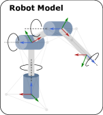

We eschew the common angle-based representation of the configuration space in favour of a distance-geometric model of robotic manipulators comprised of revolute joints [8]. This allows us to represent configurations as complete graphs . The edges are weighted by distances between a collection of points indexed by vertices , where is the workspace dimension. The coordinates of points corresponding to these distances are recovered by solving the distance geometry problem (DGP):
Distance Geometry Problem ([49]).
Given an integer , a set of vertices , and a simple undirected graph whose edges are assigned non-negative weights , find a function such that the Euclidean distances between neighbouring vertices match their edges’ weights (i.e., ).
It was shown in [9] that any solution may be mapped to a unique corresponding configuration .222Up to any Euclidean transformation of , since distances are invariant to such a transformation. Crucially, this allows us to a construct a partial graph , with corresponding to distances determined by an end-effector pose and the robot’s structure (i.e., those common to all elements of ), where each corresponds to a particular IK solution .
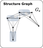
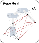
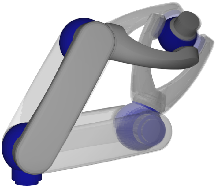
The generic procedure for constructing is demonstrated for a simple manipulator in Fig. 1. We visualize the point placement step for a pair of consecutive joints in Fig. 1(b). Two pairs of points labeled by vertices and are attached to the rotation axes of neighbouring joints at a unit distance. The edges associated with every combination of points are then weighted by their respective distances, which are defined solely by the link geometry. We build the structure graph shown in Fig. 1(c) by repeating this process for every pair of neighbouring joints. The resulting set of vertices and distance-weighted edges , shown in Fig. 1(c), describe the overall geometry and DOF of the robot because the edge weights are invariant to feasible motions of the robot (i.e., they remain constant in spite of changes to the configuration ). In order to uniquely specify points with known positions (i.e., end-effectors) in terms of distances, we define the “base vertices” , where and are the vertices in associated with the base joint. Setting the distances weighting the edges such that the points in form a coordinate frame with as the origin, we specify the edges weighted by distances between vertices in associated with the end-effector and the base vertices . The resulting subgraph , shown in Fig. 1(d), uniquely specifies an end-effector pose under the assumption of unconstrained rotation of the final joint, while is the partial graph that uniquely specifies the associated IK problem.
III-C Feature Representation for Learning
To train our GNN-based model, we must choose a representation for the partial graphs , representing the IK problem, and complete graphs , representing associated solution configurations. For a complete graph , we define the GNN node (vertex) features as a combination of point positions and general features , where each is a feature vector containing extra information about the node. For GGIK, we use a three-dimensional one-hot-encoding, and , that indicates whether the node defines the base coordinate system, a general joint or link, or the end-effector. Similarly, we use the known point positions of the partial graph as respective node features and set the remaining unknown node positions to zero. The partial graph shares the same general features as the complete graph, given that we know which part of the robot each node belongs to in advance. In both cases, the edge features are simply the corresponding inter-point distances between known node point positions. The unknown edges in the partial graph are also initialized as zeros. We note that the node feature encoding offers significant flexibility. For example, we could add an extra class or dimension to the general feature vector to indicate nodes that represent obstacles in the task space.
IV Methodology
GGIK is a learning-based IK solver that is, crucially, capable of producing multiple diverse solutions while also generalizing across a family of kinematic structures. In this section, we cover our learning procedure and our GNN network architecture in detail.
IV-A Learning to Generate Inverse Kinematics Solutions
We consider the problem of modelling complete graphs corresponding to IK solutions given partial graphs that define the problem instance (i.e., the robot’s geometric information and the task space goal pose). Intuitively, we would like our network to map or “complete” partial graphs into full graphs. Since multiple or infinite solutions may exist for a single task space goal and robot structure, a single partial graph may be associated with multiple or even infinite valid complete graphs. We interpret the learning problem through the lens of generative modelling and treat the solution space as a multimodal distribution conditioned on a single problem instance. By sampling this distribution, we are able generate diverse solutions that approximately cover the space of feasible configurations.
A visual overview of the training procedure is shown in Fig. 2. At its core, GGIK is a CVAE model [50] that parameterizes the conditional distribution using GNNs. By introducing an unobserved stochastic latent variable , our generative model is defined as
| (3) |
where is the likelihood of the full graph, is the prior, and are the learnable generative parameters. The likelihood is given by
| (4) |
where are the positions of all nodes, are the latent embeddings of each node, and are the predicted means of the distribution of node positions. We parametrize the likelihood distribution with a GNN decoder, in other words, is the output of . The GNN decoder propagates messages and updates the nodes at each intermediate layer and outputs the predicted means of all node positions at the final layer. In practice, for the input node features of , we concatenate the latent embeddings with the respective position features of the original partial graph when available and the general features . If unavailable, we concatenate the latent embeddings with the initialized position features set to zero. We follow the common practice of only learning the mean of the decoded Gaussian likelihood distribution and use a fixed diagonal covariance matrix [51]. The prior distribution is given by
| (5) |
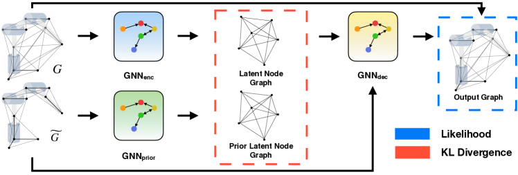
Here, we parameterize the prior as a Gaussian mixture model with components. Each Gaussian is in turn parameterized by a mean , diagonal covariance , and a mixing coefficient , where . We chose a mixture model to have an expressive prior capable of capturing the latent distribution of multiple solutions. We parameterize the prior distribution with a multi-headed GNN encoder that outputs parameters .
The goal of learning is to maximize the marginal likelihood or evidence of the data as shown in Eq. 3. As commonly done in the variational inference literature [52], we instead maximize a tractable evidence lower bound (ELBO):
| (6) |
where is the Kullback-Leibler (KL) divergence and is the inference model with learnable parameters , defined as
| (7) |
As with the prior distribution, we parameterize the inference distribution with a multi-headed GNN encoder, , that outputs parameters and . The inference model is an approximation of the intractable true posterior . We note that the resulting ELBO objective in Eq. 6 is based on an expectation with respect to the inference distribution , which itself is based on the parameters . Since we restrict to be a Gaussian variational approximation, we can use stochastic gradient descent (i.e., Monte Carlo gradient estimates) via the reparameterization trick [52] to optimize the lower bound with respect to parameters and .
At test time, given a goal pose and the manipulator’s geometric information encapsulated in a partial graph , we can use the prior network, , to encode the partial graph as a latent distribution . During training, the distribution is optimized to be simultaneously near multiple encodings of valid solutions by way of the KL divergence term in Eq. 6. We can sample this multimodal distribution as many times as needed, and subsequently decode all of the samples with the decoder network to generate IK solutions represented as complete graphs. This procedure can be done quickly and in parallel on the GPU. We provide a more detailed explanation of the sampling procedure in Section IV-C. At present, we do not consider joint limits, self-collisions, or obstacle avoidance—we simply sample randomly. However, these constraints can be incorporated into the distance-geometric formulation of IK [9, 30]; we return to this point in Section VI.
IV-B Equivariant Network Architecture
In this section, we discuss the choice of architecture for networks , , and . Recall that we are interested in mapping partial graphs into full graphs . In other words, our model maps partial point sets to full point sets , where is a combination of networks and applied sequentially. The point positions (i.e., and ) of each node in the distance geometry problem contain underlying geometric relationships and symmetries that we would like to preserve with our choice of architecture. Most importantly, the point sets are equivariant to the Euclidean group of rotations, translations, and reflections. Let be a transformation consisting of some combination of rotations, translations and reflections on the initial partial point set . Then, there exists an equivalent transformation on the complete point set such that:
| (8) |
As a specific example, if we translate a point set by , and let be shorthand for , then:
| (9) |
In other words, if we translate our initial partial graph, which defines the IK problem, then the complete graph, which defines the solution, will be equivalently translated. To leverage this structure or geometric prior in the data, we use -equivariant graph neural networks (EGNNs) [53] for , , and . The EGNN layer splits up the node features into an equivariant coordinate or position-based part and a non-equivariant part. We treat the positions and as the equivariant portion and the general features as non-equivariant. As an example, a single EGNN layer from is then defined as:
| (10) |
where, with a message embedding dimension of , , divides the sum by the number of elements, and and are typical edge and node operations approximated by multilayer perceptrons (MLPs). For more details about the model and a proof of the equivariance property, we refer readers to [53]. We present ablation studies on the use of the EGNN network architecture in Section V, indicating its importance to our approach.
IV-C Sampling Inverse Kinematics Solutions
We summarize the full sampling procedure in Algorithm 1. We first sample sets of latent variables from a Gaussian distribution parameterized by outputs from the prior encoder . The samples are then passed to the decoder network , producing point sets sampled from the distribution . Next, joint configuration (i.e., joint angle) estimates are recovered from the point sets using a simple geometric procedure described in [9]. Finally, we select the best configuratons according to some criteria. We choose to filter for the configurations with the lowest error with respect to the goal pose
Note that the configuration recovery and filtering steps may be performed in parallel for all configurations, in which case they require approximately 5 ms of computation time on a laptop CPU for . For more details on the total computation time required, see Section V-G.
V Experiments
In this section, we first cover how we generate our dataset. We then aim to (i) evaluate GGIK’s capability to learn accurate solutions and generalize within a class of manipulator structures, (ii) determine whether GGIK can be used effectively to initialize local numerical IK solvers, and (iii) investigate the importance of our choice of learning architecture. Finally, we evaluate the scaling of the computation time of a forward pass as a function of the number of samples and provide practical training advice. All experiments were performed on a laptop computer with a six-core 2.20 GHz Intel i7-8750H CPU and an NVIDIA GeForce GTX 1050 Ti Mobile GPU.
V-A Training Data
Acquiring training data is convenient—any valid manipulator configuration can be used for training. In our experiments, we use training data from two different datasets. The first dataset comprised of IK problems for existing commercial manipulators with typical kinematic structures. The second dataset contains IK problems for manipulators with randomly generated kinematic structures. In both datasets, IK ‘instances’ are generated by randomly sampling a set of joint angles and using forward kinematics to compute the associated end-effector pose. The end-effector pose is then used as the goal for IK, which ensures that all problems are feasible (i.e., have at least one solution).
Commercial manipulator dataset
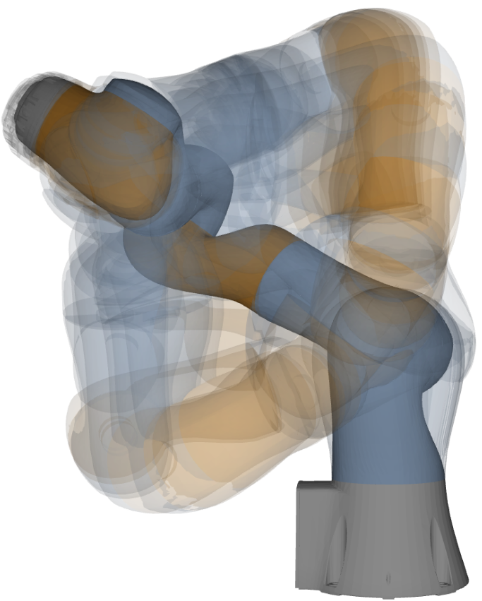
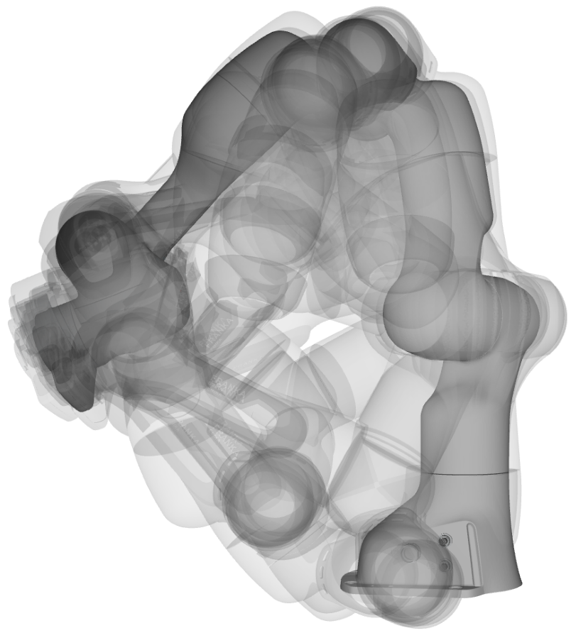
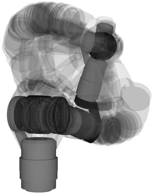
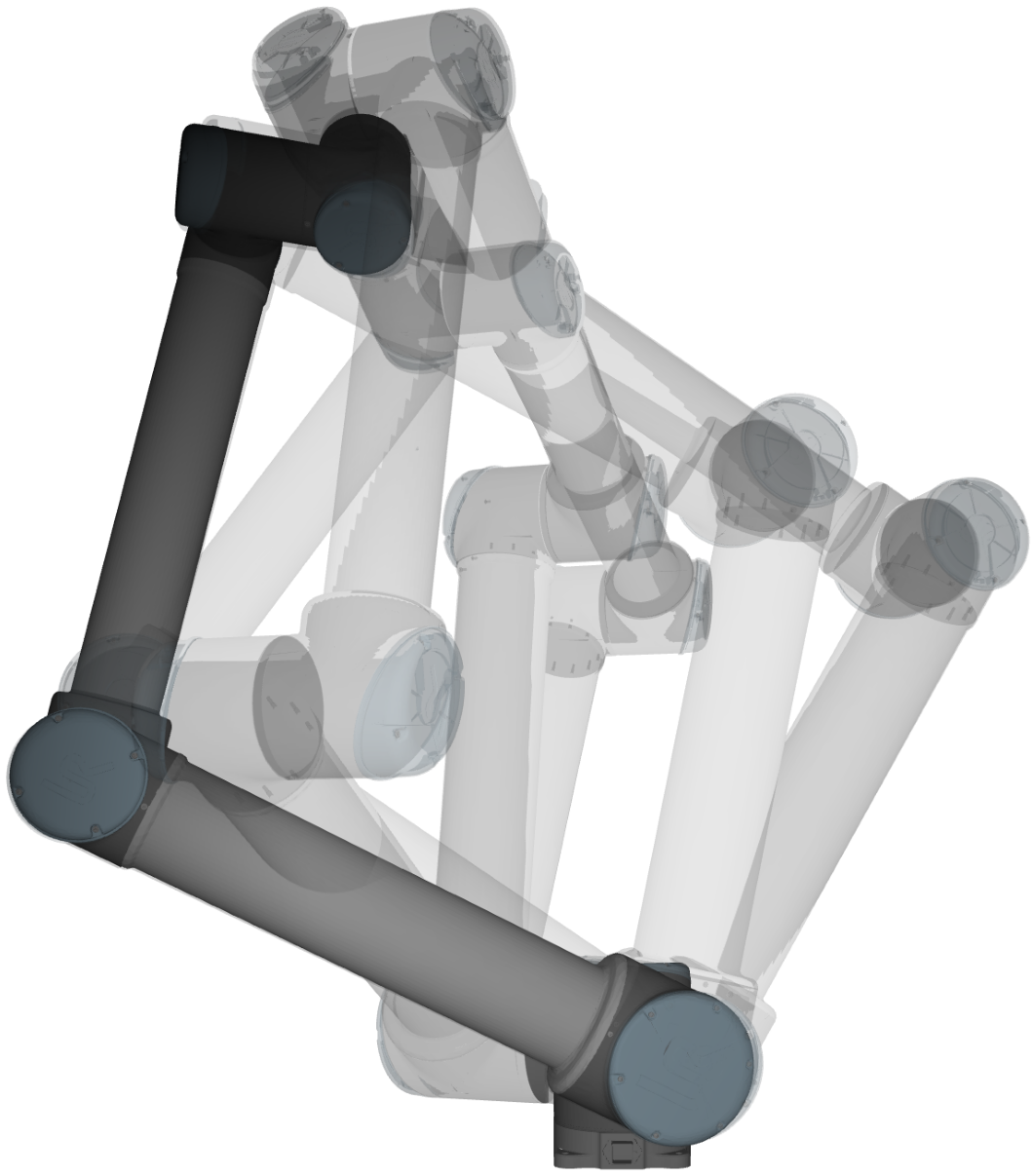
This dataset contains IK problems that are uniformly distributed over five different robots with a variety of kinematic properties. Specifically, we chose the Universal Robots UR10, Schunk LWA4P, Schunk LWA4D, KUKA IIWA and the Franka Emika Panda robots. The UR10 and LWA4P are 6 DOF robots with up to 16 discrete IK solutions for a given goal pose. On the other hand, the IIWA, LWA4D and the Panda robots all share a redundant kinematic structure with 7 DOF and, by extension, an infinite solution set to any feasible IK problem. The kinematic models for these robots are computed by parsing their respective URDF files, which allows us to render solutions generated by our model, as shown in Fig. 3.
Randomized manipulator dataset
This dataset contains a large number of randomly generated pairs of robots and associated IK problems. A unique robot was created for each problem. A key consideration for any randomization scheme used to produce such a dataset is that most real manipulators exist within a narrow class of kinematic structures. For example, the rotation axes of consecutive joints for many manipulators are either parallel or perpendicular. Furthermore, manipulators generally do not feature more than two sequential joints with parallel rotation axes, and these joints are generally displaced along a direction orthogonal to their axis of rotation. Therefore, we generate samples by randomizing DH parameters following the original convention of [48] using the procedure in Algorithm 2. This procedure accounts for regularities in kinematic structures of manipulators by sampling DH parameters from a mix of continuous and discrete distributions conditioned upon previous joints, which allows us to train models that generalize within the desired class of manipulators using a relatively small dataset. The resulting problems are constrained to robots with structures similar, but never identical to the commercial robots used in the first dataset.
V-B Accuracy
Robot Err. Pos. [mm] Err. Rot. [deg] Success [%] mean min max Q1 Q3 mean min max Q1 Q3 KUKA 5.3 1.8 9.6 3.8 6.6 0.4 0.1 0.6 0.3 0.5 100.0 Lwa4d 4.3 1.3 8.1 3.0 5.4 0.4 0.1 0.6 0.3 0.5 100.0 Lwa4p 3.8 1.6 6.5 2.9 4.7 0.3 0.1 0.4 0.2 0.4 99.6 Panda 5.8 1.6 11.1 4.0 7.4 0.4 0.1 0.7 0.3 0.5 100.0 UR10 5.5 2.7 8.6 4.4 6.6 0.3 0.1 0.5 0.2 0.4 95.3 UR10 with DT [1] 35.0 - - - - 16.0 - - - - - Panda with IKFlow [5] 7.7 - - - - 2.8 - - - - - Panda with IKNet [37] 31.0 - - 13.5 48.6 - - - - - -
Err. Pos. [mm] Err. Rot. [deg] Success [%] mean min max Q1 Q3 mean min max Q1 Q3 Robot KUKA 5.3 1.7 9.7 3.8 6.6 0.4 0.1 0.6 0.3 0.5 100.0 Lwa4d 4.7 1.4 9.1 3.2 5.9 0.4 0.1 0.6 0.3 0.5 100.0 Lwa4p 5.7 2.2 10.2 4.1 7.1 0.4 0.1 0.7 0.3 0.6 99.5 Panda 12.3 3.2 25.5 7.9 15.9 1.0 0.2 1.8 0.7 1.3 98.8 UR10 9.2 4.2 14.7 7.3 11.1 0.5 0.2 0.9 0.4 0.7 93.5
In this set of experiments, we evaluate the accuracy of GGIK for a variety of existing commercial manipulators featuring different structures and numbers of joints: the Kuka IIWA, Schunk LWA4D, Schunk LWA4P, Universal Robots UR10, and Franka Emika Panda.
Individual robots
We begin by training a model for each of the robots on 512,000 data points (IK problems) generated using the procedure described in Section V-A. We evaluate these models on 2,000 randomly generated IK problems per robot and report the errors between computed and goal end-effector poses, where the orientation error measures the magnitude of the angle in the axis-angle representation of the difference in orientation. The results in Table I show that GGIK generates solution configurations with a mean position error under 6 mm and a mean orientation error under 0.4 degrees. Moreover, the first () and third () quartile of the error distributions, as well as the maximum error values, show that the majority of sampled configurations produce end-effector poses that do not substantially deviate from the mean errors. Success rates are computed by determining whether any of the 32 samples drawn from the learned distribution for each goal pose are within a tolerance of 1 cm position error and 1 degree orientation error. We chose these tolerance bounds because they are compatible with the accuracy requirements for many human-scale tasks and would likely generate solutions in the basin of convergence of local solvers. Overall, these results indicate that, when trained on a particular manipulator, GGIK has the ability to produce solutions with an accuracy sufficient for common manipulation tasks such as grasping, pushing and obstacle avoidance.
As a benchmark, we trained a comparably-sized network on 100,000 UR10 poses using the distal teaching (DT) method of [1]. The DT network was only able to achieve a mean position error of 35 mm and a mean rotation error of 16 degrees. Moreover, this network only maps a single fixed solution to an end-effector pose, as it does not model the entire solution set—multiple calls to the network will always produce the same solution. We also compare the performance of GGIK with results reported from the IKFlow [5] and IKNet [37] models on the Franka Emika Panda manipulator. GGIK achieves a better overall accuracy than IKFlow with approximately 2 mm less translational error and 2 degrees less rotational error on average. It is also important to note that the IKFlow model is trained on 2.5 million problems per robot, roughly five times more than GGIK in Table I. GGIK achieves significantly better accuracy than IKNet, with approximately 25 mm less translational error on average. The authors of IKNet did not report on rotational errors.
Multiple robots
Next, we train a single instance of GGIK on a total of 2,560,000 IK problems uniformly distributed over all five manipulators, that is, a single model for multiple robots. The model is evaluated on 10,000 randomly generated feasible IK problems (2,000 per robot). The success rates in Table II suggest that the proposed approach is feasible for generating solutions in a variety of practical applications. The somewhat lower success rates for the UR10 and Panda robots are likely caused by their structural distinctness from the relatively similar kinematic structures of the remaining robots. This could induce a bias towards the Kuka IIWA, LWA4D and LWA4P, as there exists a higher degree of transferability between model parameters that minimize the associated loss terms. One possibility to mitigate this issue could be to modify the distribution of examples within the training set to compensate, which we leave for future investigation. The results shown in Fig. 4 indicate that by simply increasing the number of samples, the gap in solution accuracy between the various manipulators is reduced
robot using our standard procedure with 256,000 random training samples (robot configurations) of the Panda manipulator.
V-C Generalization
Err. Pos. [mm] Err. Rot. [deg] Success [%] mean min max Q1 Q3 mean min max Q1 Q3 Robot KUKA 39.7 11.4 75.5 27.8 50.4 2.5 0.5 4.6 1.7 3.3 44.0 Lwa4d 35.7 10.2 68.3 25.0 45.5 2.3 0.5 4.3 1.6 3.1 53.1 Lwa4p 22.5 7.3 40.4 16.3 28.2 1.5 0.4 2.6 1.0 1.9 80.0 UR10 46.5 22.1 69.7 37.9 55.3 2.0 0.6 3.5 1.4 2.5 26.9
In order to determine the capacity of GGIK to generalize to unseen manipulator structures, we evaluate the accuracy of the trained model on robots outside of the training set. To this end, we generate a dataset of inverse kinematics problems for manipulators with randomized kinematic structures, following the procedure outlined in Section V-A. The training set consists of 4,096,000 inverse kinematics problems, each for a unique six or seven DOF robot generated using randomized DH parameters (i.e., no two robots in the dataset are identical). Batches of 128 robots are randomly selected during training, independently of their DOF and structure. The robots and procedure used in evaluation are identical to the experiment presented in Section V-B. Results are presented in Table III, where each line in the table shows results from 2,000 IK problems solved by the trained model.
Our learned model is able to generalize reasonably well across all robots, reaching a mean position error of approximately 2 to 4 cm and a mean orientation error of 2 degrees. In contrast to the model trained on specific robots discussed in Section V-B, this model exchanges accuracy for the capability to generate approximate solutions for a much larger variety of robots. While the accuracy of this model is not sufficient alone for some practical use cases, the results in Section V-E suggest that the approximate solutions it provides can be refined by a few iterations of a local optimization procedure.
V-D Multimodality
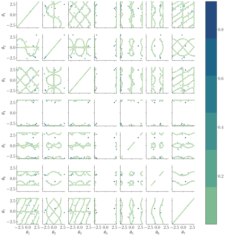
In addition to providing accurate solutions, GGIK is able to uniformly sample the entire set of feasible configurations for a given goal pose. This capability can be understood qualitatively by plotting pairs of joint angle variables for multiple solutions sampled from GGIK for a single query. An example of this visualization procedure for 1,000 samples for the Kuka arm is displayed in Fig. 5. Each of the plots in the symmetric upper and lower triangles of the array in Fig. 5 contains the sampled joint angles for a pair and . Since each pair contains samples from the torus , the and axes “wrap around” at . The hue of each sample is based on its pose error, with darker samples indicating less accurate solutions. The continuous and orderly curves produced by accurate solutions indicate that GGIK is able to learn a relatively complex distribution over a large, varied solution set.
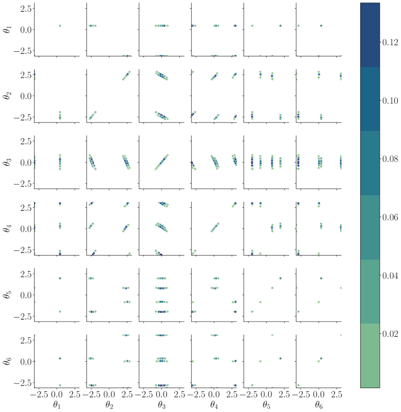
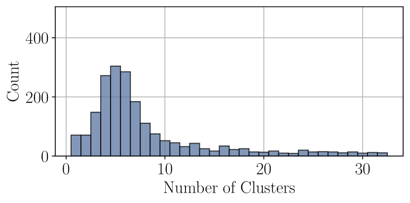
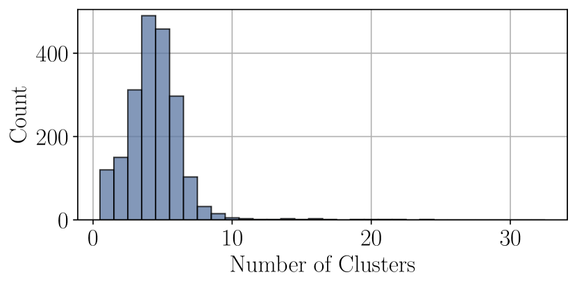
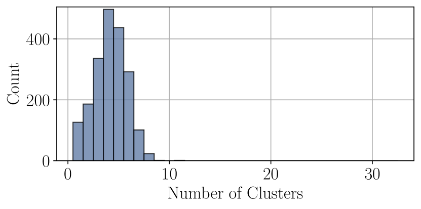
Since the UR10 is a (non-redundant) 6-DOF manipulator, we expect the same visualization for this arm to consist of discrete clusters. Fig. 6 demonstrates that this is indeed the case, with an interesting phenomenon occurring for this particular goal pose: the less accurate samples from GGIK appear to be attempts at interpolating between high accuracy clusters (i.e., those with lighter colouring). This does not occur for all poses sampled, and a quantitative clustering experiment confirms that GGIK is in fact learning a few accurate clusters for most poses. Using 32 GGIK samples for each of 2,000 random goal poses, we computed a Density-Based Spatial Clustering of Applications with Noise (DBSCAN) [54] using the product metric of the chordal distance for . DBSCAN was selected because it supports data on topological manifolds and has very few parameters to tune. Fig. 7 contains histograms displaying the distribution of the number of clusters recovered by DBSCAN with a variety of values for the radius parameter . In all three cases, the minimum cluster size was set to one in order to allow for clusters containing a single sample. Ideally, we would like to see the number of clusters concentrated around eight, which is the maximum number of solutions for the UR10. In Fig. 7(a), is small and noisy clusters are erroneously separated. However, the similarity between the distributions in Fig. 7(b) and Fig. 7(c) indicates that this is a fairly stable clustering procedure. Indeed, in both histograms there are very few poses for which GGIK produced greater than eight clusters, while the median number of clusters is four. Whether our approach can be modified to consistently produce the maximum number of solutions possible in the case of 6 DOF manipulators remains to be seen, but the results in Fig. 7 show that our current model does not learn distributions concentrated around a single solution.
V-E Initializing Numerical Solvers
Initialization Err. Pos. [mm] Err. Rot. [deg] Num. Iter. Time [ms] Success [%] mean min max Q1 Q3 mean min max Q1 Q3 mean std mean std SQP + rand 3.5 0.0 144.1 0.1 0.2 0.0 0.0 0.8 0.0 0.0 29.3 11.3 104.9 44.6 95.0 SQP + GGIK 0.7 0.0 8.7 0.1 0.7 0.0 0.0 0.1 0.0 0.0 10.9 4.4 39.8 14.9 100.0 GRAPHIK + rand 30.5 0.0 173.2 21.1 38.1 1.8 0.0 11.5 1.0 2.0 182.7 142.1 287.0 251.5 80.7 GRAPHIK + GGIK 0.2 0.0 9.1 0.1 0.2 0.0 0.0 0.4 0.0 0.0 84.0 109.9 192.6 237.1 99.9
GGIK learns a sampling distribution capable of producing multiple approximate solutions in parallel, which may be used as initializations for optimization-based methods. Table IV shows the results of repeating the experiment in Section V-B using an IK solver based on the SLSQP algortihm implemented in the scipy.optimize package [55], setting a maximum of 100 iterations and keeping other termination criteria at their default values. We compare the accuracy and number of iterations required by the solver before convergence when initialized with 32 random configurations per problem and 32 samples from our learned distribution. We average the results over all problems and all robots. While both approaches achieve a high degree of success and accuracy on these unconstrained problems, the results clearly show that using our model to initialize the optimization yields better overall performance. Specifically, the mean number of iterations required compared to random initializations is almost three times lower, and the accuracy of the solutions is notably higher as well. In difficult or highly constrained instances of IK, our model could be used as a way to provide a large number of informed initializations that are close to the solution manifold.
V-F Ablation Study on the Equivariant Network Architecture
Model Name Err. Pos. [mm] Err. Rot. [deg] Test ELBO Success [%] mean min max Q1 Q3 mean min max Q1 Q3 EGNN 4.6 1.5 8.5 3.3 5.8 0.4 0.1 0.6 0.3 0.4 -0.05 99.8 MPNN 143.2 62.9 273.7 113.1 169.1 17.7 5.3 13.6 21.6 34.1 -8.3 13.1 GAT - - - - - - - - - - -12.41 0.0 GCN - - - - - - - - - - -12.42 0.0 GRAPHsage - - - - - - - - - - -10.5 0.0
We conducted an ablation experiment to evaluate the importance of capturing the underlying equivariance of graphical IK in our learning architecture. We compare the use of the EGNN network [53] to four common and popular GNN layers that are not equivariant: GRAPHsage [56], GAT [57], GCN [58] and MPNN [59]. We match the number of parameters for each GNN architecture as closely as possible and keep all other experimental parameters fixed. Our dataset is the same one used in Section V-B, however the results are averaged over all manipulators as shown in Table V. Out of the five different architectures that we compare, only the EGNN and MPNN output point sets that can be successfully mapped to valid joint configurations. Point sets that are too far from those representing a valid joint configuration result in the configuration reconstruction procedure diverging. The equivariant EGNN model outperforms all other models in terms of the ELBO value attained and overall solution accuracy on a held-out test set.
V-G Time Taken to Generate Multiple Samples
We studied the scaling of the computation time as a function of the number of solution samples generated by GGIK. Batched requests can take advantage of the GPU architecture and yield very low per-solution solve times when amortized across larger batches. This could be used, for example, in sampling-based motion planning and workspace analysis. The results displayed in Fig. 8 demonstrate that GGIK is able to generate 10 samples in 10 milliseconds and 1,000 samples in 80 milliseconds.
V-H Training Details
We provide some brief and practical advice for training GGIK, based on our experimental observations. Picking a network architecture that captures the underlying geometry and equivariance of the problem improved the training by a large margin as shown by Table V. By far, the choice of GNN architecture had the most impact on the performance of our models. In order to increase the accuracy of our models, we found it particularly effective to lower the learning rate when the training loss stagnated. We empirically observed that increasing the number of layers in our GNNs up to five improved the overall performance. There was very little performance improvement beyond five layers. We found that using a mixture model for the distribution of the prior encoder lead to more accurate results. We hypothesize that a more expressive prior distribution can better fit multiple encoded IK solutions when conditioned on a single goal pose. Finally, we found that lowering the weight of the reconstruction loss or likelihood contribution from nodes that belonged to the structure graph (see Section III-B) led to overall lower losses. We used SiLU non-linearities [60] with layer normalization [61] and Adam with weight decay [62] and a learning rate of 3e-4. For more implementation details, we invite interested readers to refer to the open-source code.
VI Future Work
While our proposed architecture demonstrates a capacity for generalization and an ability to produce diverse solutions, GGIK outputs may require post-processing by local optimization methods in applications that require low tolerances for error. As interesting future work, we would like to learn constrained distributions of robot configurations that account for obstacles in the task space and for self-collisions; obstacles can be easily incorporated in the distance-geometric representation of IK [9, 30] as nodes. In particular, self-collisions are often addressed by enforcing joint limits, allowing us to avoid this problem by efficiently filtering the resulting configuration samples. Nevertheless, this problem may also be addressed by carefully curating collision-free configurations for the training set or by adding associated loss terms. Learning an obstacle- and collision-aware distribution would yield a solver that implements collision avoidance by way of message passing between manipulator and obstacle nodes.
VII Conclusion
We have presented GGIK, a generative graphical IK solver that is able to produce multiple diverse and accurate solutions in parallel across many different manipulator types. This capability is achieved through a distance-geometric representation of the IK problem in concert with GNNs and generative modelling. The accuracy of the generated solutions points to the potential of GGIK as both a standalone solver and as an initialization method for local optimization methods. To the best of our knowledge, this is the first approach capable of learning a model which can generate multiple solutions for robots not present in the training set. Importantly, because GGIK is fully differentiable, it can be incorporated as a flexible IK component that is part of an end-to-end learning-based robotic manipulation framework. GGIK provides a framework for learned general IK—a universal solver (or initializer) that can provide multiple diverse solutions for any manipulator structure in a way that complements or replaces numerical optimization.
References
- [1] T. von Oehsen, A. Fabisch, S. Kumar, and F. Kirchner, “Comparison of Distal Teacher Learning with Numerical and Analytical Methods to Solve Inverse Kinematics for Rigid-Body Mechanisms,” arXiv:2003.00225 [cs], Feb. 2020.
- [2] A. Aristidou, J. Lasenby, Y. Chrysanthou, and A. Shamir, “Inverse Kinematics Techniques in Computer Graphics: A Survey,” Computer Graphics Forum, vol. 37, no. 6, pp. 35–58, Sep. 2018.
- [3] H. Ren and P. Ben-Tzvi, “Learning inverse kinematics and dynamics of a robotic manipulator using generative adversarial networks,” Robotics and Autonomous Systems, vol. 124, p. 103386, 2020.
- [4] C.-K. Ho and C.-T. King, “Selective inverse kinematics: A novel approach to finding multiple solutions fast for high-dof robotic,” arXiv preprint arXiv:2202.07869, 2022.
- [5] B. Ames, J. Morgan, and G. Konidaris, “Ikflow: Generating diverse inverse kinematics solutions,” IEEE Robotics and Automation Letters, vol. 7, no. 3, pp. 7177–7184, 2022.
- [6] T. S. Lembono, E. Pignat, J. Jankowski, and S. Calinon, “Learning constrained distributions of robot configurations with generative adversarial network,” IEEE Robotics and Automation Letters, vol. 6, no. 2, pp. 4233–4240, 2021.
- [7] P. Beeson and B. Ames, “TRAC-IK: An open-source library for improved solving of generic inverse kinematics,” in 15th International Conf. on Humanoid Robots (Humanoids). IEEE, 2015, pp. 928–935.
- [8] J. Porta, L. Ros, F. Thomas, and C. Torras, “A branch-and-prune solver for distance constraints,” IEEE Trans. Robot., vol. 21, pp. 176–187, Apr. 2005.
- [9] F. Maric, M. Giamou, A. W. Hall, S. Khoubyarian, I. Petrovic, and J. Kelly, “Riemannian optimization for distance-geometric inverse kinematics,” IEEE Transactions on Robotics, 2021. [Online]. Available: https://arxiv.org/abs/2108.13720
- [10] H.-Y. Lee and C.-G. Liang, “A new vector theory for the analysis of spatial mechanisms,” Mech. Mach. Theory, vol. 23, no. 3, pp. 209–217, 1988.
- [11] D. Manocha and J. F. Canny, “Efficient inverse kinematics for general 6r manipulators,” IEEE Trans. Robot.
- [12] M. Husty, M. Pfurner, and H. Schröcker, “A new and efficient algorithm for the inverse kinematics of a general serial 6r manipulator,” Mech. Mach. Theory, vol. 42, no. 1, pp. 66–81, 2007.
- [13] R. Diankov, “Automated construction of robotic manipulation programs,” Ph.D. dissertation, Carnegie Mellon University, Pittsburgh, PA, September 2010.
- [14] D. E. Whitney, “Resolved motion rate control of manipulators and human prostheses,” IEEE Transactions on man-machine systems, vol. 10, no. 2, pp. 47–53, 1969.
- [15] L. Sciavicco and B. Siciliano, “Coordinate transformation: A solution algorithm for one class of robots,” vol. 16, no. 4, pp. 550–559, 1986.
- [16] Y. Nakamura, H. Hanafusa, and T. Yoshikawa, “Task-priority based redundancy control of robot manipulators,” Int. J. Rob. Res., vol. 6, no. 2, pp. 3–15, 1987.
- [17] K. M. Lynch and F. C. Park, Modern robotics. Cambridge University Press, 2017.
- [18] B. Siciliano, L. Sciavicco, L. Villani, and G. Oriolo, Robotics: Modelling, Planning and Control. Springer Science & Business Media, 2010.
- [19] R. Tedrake, Robotic Manipulation, 2022. [Online]. Available: http://manipulation.mit.edu
- [20] M. Engell-Nørregrd and K. Erleben, “A projected non-linear conjugate gradient method for interactive inverse kinematics,” in MATHMOD 2009-6th Vienna International Conference on Mathematical Modelling, 2009.
- [21] A. S. Deo and I. D. Walker, “Adaptive non-linear least squares for inverse kinematics,” in Proceedings IEEE International Conference on Robotics and Automation. IEEE, 1993, pp. 186–193.
- [22] K. Erleben and S. Andrews, “Solving inverse kinematics using exact Hessian matrices,” Comput. Graph., vol. 78, pp. 1–11, Feb. 2019.
- [23] S. Boyd and L. Vandenberghe, Convex Optimization. Cambridge University Press, 2004.
- [24] B. Kenwright, “Inverse kinematics–cyclic coordinate descent (CCD),” J. Graphics Tools, vol. 16, no. 4, pp. 177–217, 2012.
- [25] A. Aristidou and J. Lasenby, “FABRIK: A fast, iterative solver for the inverse kinematics problem,” Graph. Models, vol. 73, no. 5, p. 243–260, Sep. 2011.
- [26] J. G. de Jalón, “Twenty-five years of natural coordinates,” Multibody Sys. Dyn., vol. 18, no. 1, pp. 15–33, Aug. 2007.
- [27] H. Dai, G. Izatt, and R. Tedrake, “Global inverse kinematics via mixed-integer convex optimization,” Int. J. Rob. Res., vol. 38, no. 12-13, pp. 1420–1441, Oct. 2019.
- [28] T. Yenamandra, F. Bernard, J. Wang, F. Mueller, and C. Theobalt, “Convex Optimisation for Inverse Kinematics,” Proc. Int. Conf. 3D Vision (3DV), pp. 318–327, Sep. 2019.
- [29] T. Le Naour, N. Courty, and S. Gibet, “Kinematics in the metric space,” Comput. Graph., vol. 84, pp. 13–23, 2019.
- [30] M. Giamou, F. Maric, D. M. Rosen, V. Peretroukhin, N. Roy, I. Petrovic, and J. Kelly, “Convex iteration for distance-geometric inverse kinematics,” IEEE Robotics and Automation Letters, 2022, to Appear. [Online]. Available: https://arxiv.org/abs/2109.03374
- [31] M. I. Jordan and D. E. Rumelhart, “Forward models: Supervised learning with a distal teacher,” Cognitive science, vol. 16, no. 3, pp. 307–354, 1992.
- [32] A. D’Souza, S. Vijayakumar, and S. Schaal, “Learning inverse kinematics,” in Proceedings 2001 IEEE/RSJ International Conference on Intelligent Robots and Systems. Expanding the Societal Role of Robotics in the the Next Millennium (Cat. No. 01CH37180), vol. 1. IEEE, 2001, pp. 298–303.
- [33] B. Bócsi, D. Nguyen-Tuong, L. Csató, B. Schoelkopf, and J. Peters, “Learning inverse kinematics with structured prediction,” in 2011 IEEE/RSJ International Conference on Intelligent Robots and Systems. IEEE, 2011, pp. 698–703.
- [34] R. Villegas, J. Yang, D. Ceylan, and H. Lee, “Neural Kinematic Networks for Unsupervised Motion Retargetting,” ArXiv180405653 Cs, Apr. 2018.
- [35] L. Ardizzone, J. Kruse, C. Rother, and U. Köthe, “Analyzing inverse problems with invertible neural networks,” in International Conference on Learning Representations, 2018.
- [36] J. Kruse, L. Ardizzone, C. Rother, and U. Köthe, “Benchmarking invertible architectures on inverse problems,” arXiv preprint arXiv:2101.10763, 2021.
- [37] R. Bensadoun, S. Gur, N. Blau, and L. Wolf, “Neural inverse kinematic,” in Proceedings of the 39th International Conference on Machine Learning, ser. Proceedings of Machine Learning Research, K. Chaudhuri, S. Jegelka, L. Song, C. Szepesvari, G. Niu, and S. Sabato, Eds., vol. 162. Baltimore, Maryland, USA: PMLR, July 2022, pp. 1787–1797.
- [38] J. Ichnowski, Y. Avigal, V. Satish, and K. Goldberg, “Deep learning can accelerate grasp-optimized motion planning,” Science Robotics, vol. 5, no. 48, p. eabd7710, 2020.
- [39] A. Khan, A. Ribeiro, V. Kumar, and A. G. Francis, “Graph neural networks for motion planning,” arXiv preprint arXiv:2006.06248, 2020.
- [40] B. Ichter, J. Harrison, and M. Pavone, “Learning sampling distributions for robot motion planning,” in 2018 IEEE International Conference on Robotics and Automation (ICRA). IEEE, 2018, pp. 7087–7094.
- [41] A. H. Qureshi, Y. Miao, A. Simeonov, and M. C. Yip, “Motion planning networks: Bridging the gap between learning-based and classical motion planners,” IEEE Transactions on Robotics, vol. 37, no. 1, pp. 48–66, 2020.
- [42] R. Liao, “Graph neural networks: Graph generation,” in Graph Neural Networks: Foundations, Frontiers, and Applications, L. Wu, P. Cui, J. Pei, and L. Zhao, Eds. Singapore: Springer Singapore, 2022, pp. 225–250.
- [43] T. N. Kipf and M. Welling, “Variational graph auto-encoders,” arXiv preprint arXiv:1611.07308, 2016.
- [44] N. De Cao and T. Kipf, “Molgan: An implicit generative model for small molecular graphs,” arXiv preprint arXiv:1805.11973, 2018.
- [45] Y. Li, O. Vinyals, C. Dyer, R. Pascanu, and P. Battaglia, “Learning deep generative models of graphs,” arXiv preprint arXiv:1803.03324, 2018.
- [46] G. N. Simm and J. M. Hernández-Lobato, “A generative model for molecular distance geometry,” arXiv preprint arXiv:1909.11459, 2019.
- [47] R. M. Murray, Z. Li, and S. S. Sastry, A mathematical introduction to robotic manipulation. CRC press, 2017.
- [48] R. S. Hartenberg and J. Denavit, “A kinematic notation for lower pair mechanisms based on matrices,” J. Appl. Mech., vol. 77, no. 2, pp. 215–221, 1955.
- [49] L. Liberti, C. Lavor, N. Maculan, and A. Mucherino, “Euclidean Distance Geometry and Applications,” SIAM Rev., vol. 56, no. 1, pp. 3–69, Jan. 2014.
- [50] K. Sohn, X. Yan, and H. Lee, “Learning structured output representation using deep conditional generative models,” in Proceedings of the 28th International Conference on Neural Information Processing Systems - Volume 2, ser. NeurIPS’15. Cambridge, MA, USA: MIT Press, 2015, pp. 3483–3491.
- [51] C. Doersch, “Tutorial on variational autoencoders,” arXiv preprint arXiv:1606.05908, 2016.
- [52] D. P. Kingma and M. Welling, “Auto-encoding variational Bayes,” in International Conference on Learning Representations, Y. Bengio and Y. LeCun, Eds., 2014.
- [53] V. G. Satorras, E. Hoogeboom, and M. Welling, “E (n) equivariant graph neural networks,” in International Conference on Machine Learning. PMLR, 2021, pp. 9323–9332.
- [54] E. Schubert, J. Sander, M. Ester, H. P. Kriegel, and X. Xu, “Dbscan revisited, revisited: why and how you should (still) use dbscan,” ACM Transactions on Database Systems (TODS), vol. 42, no. 3, pp. 1–21, 2017.
- [55] P. Virtanen, R. Gommers, T. E. Oliphant, M. Haberland, T. Reddy, D. Cournapeau, E. Burovski, P. Peterson, W. Weckesser, J. Bright, S. J. van der Walt, M. Brett, J. Wilson, K. J. Millman, N. Mayorov, A. R. J. Nelson, E. Jones, R. Kern, E. Larson, C. J. Carey, İ. Polat, Y. Feng, E. W. Moore, J. VanderPlas, D. Laxalde, J. Perktold, R. Cimrman, I. Henriksen, E. A. Quintero, C. R. Harris, A. M. Archibald, A. H. Ribeiro, F. Pedregosa, P. van Mulbregt, and SciPy 1.0 Contributors, “SciPy 1.0: Fundamental Algorithms for Scientific Computing in Python,” Nature Methods, vol. 17, pp. 261–272, 2020.
- [56] W. Hamilton, Z. Ying, and J. Leskovec, “Inductive representation learning on large graphs,” Advances in neural information processing systems, vol. 30, 2017.
- [57] P. Velickovic, G. Cucurull, A. Casanova, A. Romero, P. Lio, and Y. Bengio, “Graph attention networks,” in International Conference on Learning Representations, 2018.
- [58] T. N. Kipf and M. Welling, “Semi-Supervised Classification with Graph Convolutional Networks,” in International Conference on Learning Representations, 2017.
- [59] J. Gilmer, S. S. Schoenholz, P. F. Riley, O. Vinyals, and G. E. Dahl, “Neural message passing for quantum chemistry,” in International Conference on Machine Learning. PMLR, 2017, pp. 1263–1272.
- [60] S. Elfwing, E. Uchibe, and K. Doya, “Sigmoid-weighted linear units for neural network function approximation in reinforcement learning,” Neural Networks, vol. 107, pp. 3–11, 2018.
- [61] J. L. Ba, J. R. Kiros, and G. E. Hinton, “Layer normalization,” arXiv preprint arXiv:1607.06450, 2016.
- [62] I. Loshchilov and F. Hutter, “Decoupled weight decay regularization,” in International Conference on Learning Representations, 2019.
![[Uncaptioned image]](/html/2209.08812/assets/figures/headshots/oliver.jpeg) |
Oliver Limoyo received his B.Eng. degree in mechanical engineering from McGill University in 2016. He is currently pursuing a Ph.D. degree at the Space and Terrestrial Autonomous Robotic Systems (STARS) laboratory at the University of Toronto. His research interests include the integration of generative models for robotics, reinforcement learning and imitation learning. |
![[Uncaptioned image]](/html/2209.08812/assets/x11.jpg) |
Filip Marić Received his Ph.D. degree from the University of Toronto, Canada and University of Zagreb, Croatia in 2023. He received his B.Sc. and M.Sc. Degrees in electrical engineering and information technology from the University of Zagreb in 2015 and 2017, respectively. He is currently a senior research AI research scientist at the Samsung AI Center in Montreal, Canada. His research interests include robotic manipulation, planning and multi-modal deep learning. |
![[Uncaptioned image]](/html/2209.08812/assets/figures/headshots/matt.png) |
Matthew Giamou received his Ph.D. degree from the University of Toronto in 2023. He is currently a postdoctoral researcher at the Northeastern University Robust Autonomy Laboratory (NEURAL), where he is developing efficient convex optimization methods for large-scale robust robotic perception. His research interests also include multi-robot systems, sensor calibration, and the integration of learned and classical models for state estimation. |
![[Uncaptioned image]](/html/2209.08812/assets/figures/headshots/petra.png) |
Petra Alexson is a fourth-year Engineering Science student at the University of Toronto, specializing in electrical and computer engineering. She was an undergraduate research assistant at the Space and Terrestrial Autonomous Robotic Systems (STARS) laboratory at the University of Toronto Institute for Aerospace Studies in the summer of 2021. During her time in STARS, she investigated several machine learning-based solutions to the inverse kinematics problem. She expects to receive her B.A.Sc in 2024. |
![[Uncaptioned image]](/html/2209.08812/assets/figures/headshots/petrovic_ivan.png) |
Ivan Petrović received the Master of Science and the Ph.D. degrees from FER Zagreb, Zagreb, Croatia, in 1990 and 1998, respectively. He is a Professor and the Head of the Laboratory for Autonomous Systems and Mobile Robotics, Faculty of Electrical Engineering and Computing, University of Zagreb, Zagreb, Croatia. He has published about 60 journal and 200 conference papers. His current research interest includes advanced control and estimation techniques and their application in autonomous systems and robotics. Prof. Petrović is a Full Member of the Croatian Academy of Engineering, and the Chair of the IFAC Technical Committee on Robotics. |
![[Uncaptioned image]](/html/2209.08812/assets/figures/headshots/kelly_jonathan.png) |
Jonathan Kelly received his Ph.D. degree from the University of Southern California, Los Angeles, USA, in 2011. From 2011 to 2013 he was a postdoctoral fellow in the Computer Science and Artificial Intelligence Laboratory at the Massachusetts Institute of Technology, Cambridge, USA. He is currently an associate professor and director of the Space and Terrestrial Autonomous Robotic Systems (STARS) Laboratory, University of Toronto Institute for Aerospace Studies, Toronto, Canada. Prof. Kelly holds the Tier II Canada Research Chair in Collaborative Robotics. His research interests include perception, planning, and learning for interactive robotic systems. |