An adaptive finite element method for distributed elliptic optimal control problems with
variable energy regularization

Abstract

We analyze the finite element discretization of distributed elliptic optimal control problems with variable energy regularization, where the usual $L^{2}(\Omega)$ norm regularization term with a constant regularization parameter $\varrho$ is replaced by a suitable representation of the energy norm in $H^{-1}(\Omega)$ involving a variable, mesh-dependent regularization parameter $\varrho(x)$. It turns out that the error between the computed finite element state $\widetilde{u}_{\varrho h}$ and the desired state $\overline{u}$ (target) is optimal in the $L^{2}(\Omega)$ norm provided that $\varrho(x)$ behaves like the local mesh size squared. This is especially important when adaptive meshes are used in order to approximate discontinuous target functions. The adaptive scheme can be driven by the computable and localizable error norm $\|\widetilde{u}_{\varrho h}-\overline{u}\|_{L^{2}(\Omega)}$ between the finite element state $\widetilde{u}_{\varrho h}$ and the target $\overline{u}$. The numerical results not only illustrate our theoretical findings, but also show that the iterative solvers for the discretized reduced optimality system are very efficient and robust.

Keywords: Distributed elliptic optimal control problem, variable energy regularization, finite element discretization, error estimates, adaptivity, solvers
2010 MSC: 49J20, 49M05, 35J05, 65M60, 65M15, 65N22

1 Introduction

Optimal control [2, 12, 19, 25] and inverse problems [8, 14, 23] subject to partial differential equations often involve some parameter-dependent cost or regularization terms, see also the recent special issue [7] on optimal control and inverse problems. While in optimal control problems the regularization parameter $\varrho$ is often considered as a given constant, in inverse problems, the parameter-dependent convergence as $\varrho\to 0$ is well studied, see, e.g., [1]. For tracking type cost functionals subject to elliptic partial differential equations, the regularization error was analyzed in [21] which depends on the regularity of the given target. In [17], and in the case of energy regularization, we have considered a related finite element analysis which resulted in an optimal choice of the regularization parameter $\varrho=h^{2}$, or vice versa, where $h$ is the mesh size of the globally quasi-uniform finite element mesh. While the latter can be used to approximate smooth target functions in the state space, adaptively refined finite element meshes should be used when considering less regular target functions, e.g., discontinuous or singular, or violating Dirichlet boundary conditions which are involved in the definition of the state space. This motivates the use of a variable regularization parameter function which can be defined by using the local finite element mesh sizes $h_{\ell}$. We are not aware of any paper on optimal control problems dealing with such an approach. However, there are several papers in imaging considering a similar approach: In [13], a variable regularization parameter is used for an adaptive balancing of the data fidelity and the regularization term, see equation (3) in [13]. A variable $L^{2}(\Omega)$ (TV) regularization is considered in [6, equation (1.1)]. Finally, a spatially adapted total generalized variation model was already used in [4, equation (1.4)], see also the more recent work [11].

As model problem we consider the optimal control problem to minimize the cost functional

$${\mathcal{J}}(u_{\varrho},z_{\varrho})=\frac{1}{2}\int_{\Omega}[u_{\varrho}(x)-\overline{u}(x)]^{2}dx+\frac{1}{2}\,\varrho\,\|z_{\varrho}\|^{2}_{H^{-1}(\Omega)}$$ (1.1)

subject to the Dirichlet boundary value problem for the Poisson equation,

$$-\Delta u_{\varrho}=z_{\varrho}\quad\mbox{in}\;\Omega,\quad u_{\varrho}=0\quad\mbox{on}\;\partial\Omega.$$ (1.2)

We assume that $\Omega\subset{\mathbb{R}}^{n}$, $n=1,2,3$, is a bounded Lipschitz domain, and $\varrho\in{\mathbb{R}}_{+}$ is some, at this time constant, regularization parameter, on which the solution $(u_{\varrho},z_{\varrho})$ depends. Our particular interest is in the behavior of $\|u_{\varrho}-\overline{u}\|_{L^{2}(\Omega)}$ as $\varrho\to 0$, see [21]. Note that the energy norm as used in (1.1) is given by

$$\|z_{\varrho}\|_{H^{-1}(\Omega)}^{2}=\|\nabla u_{\varrho}\|^{2}_{L^{2}(\Omega)}=\langle z_{\varrho},u_{\varrho}\rangle_{\Omega},=\langle z_{\varrho},{\mathcal{S}}z_{\varrho}\rangle_{\Omega},$$

where $u_{\varrho}={\mathcal{S}}z_{\varrho}\in H^{1}_{0}(\Omega)$ is the weak solution of the primal Dirichlet boundary value problem (1.2), and ${\mathcal{S}}:H^{-1}(\Omega)\to H^{1}_{0}(\Omega)\subset L^{2}(\Omega)$ is the associated solution operator. Hence we can write the reduced cost functional as

$$\widetilde{\mathcal{J}}(z_{\varrho})=\frac{1}{2}\,\|{\mathcal{S}}z_{\varrho}-\overline{u}\|^{2}_{L^{2}(\Omega)}+\frac{1}{2}\,\varrho\,\langle{\mathcal{S}}z_{\varrho},z_{\varrho}\rangle_{\Omega},$$ (1.3)

and its minimizer is given as the unique solution of the gradient equation

$${\mathcal{S}}^{*}({\mathcal{S}}z_{\varrho}-\overline{u})+\varrho\,{\mathcal{S}}z_{\varrho}=0\,.$$

In addition to $u_{\varrho}={\mathcal{S}}z_{\varrho}$ we now introduce the adjoint state $p_{\varrho}={\mathcal{S}}^{*}(u_{\varrho}-\overline{u})$ as unique solution of the Dirichlet boundary value problem

$$-\Delta p_{\varrho}=u_{\varrho}-\overline{u}\quad\mbox{in}\;\Omega,\quad p_{\varrho}=0\quad\mbox{on}\;\partial\Omega.$$ (1.4)

Hence we can rewrite the gradient equation as

$$p_{\varrho}+\varrho\,u_{\varrho}=0\quad\mbox{in}\;\Omega.$$

When eliminating the adjoint state $p_{\varrho}$ we can determine the optimal state $u_{\varrho}$ as the solution of the singularly perturbed Dirichlet boundary value problem

$$-\varrho\,\Delta u_{\varrho}+u_{\varrho}=\overline{u}\quad\mbox{in}\;\Omega,\quad u_{\varrho}=0\quad\mbox{on}\;\partial\Omega,$$ (1.5)

which is also known as differential filter in fluid mechanics [15]. The variational formulation of (1.5) is to find $u_{\varrho}\in H^{1}_{0}(\Omega)$ such that

$$\varrho\,\langle\nabla u_{\varrho},\nabla v\rangle_{L^{2}(\Omega)}+\langle u_{\varrho},v\rangle_{L^{2}(\Omega)}=\langle\overline{u},v\rangle_{L^{2}(\Omega)}\quad\mbox{for all}\;v\in H^{1}_{0}(\Omega).$$ (1.6)

For a finite element discretization of the variational formulation (1.5) we may use the ansatz space $V_{h}:=S_{h}^{1}(\Omega)\cap H^{1}_{0}(\Omega)$ of piecewise linear and continuous basis functions which are defined with respect to some admissible and globally quasi-uniform decomposition of $\Omega$ into simplicial finite elements of mesh size $h$. The Galerkin variational formulation of (1.6) is to find $u_{\varrho h}\in V_{h}$ such that

$$\varrho\,\langle\nabla u_{\varrho h},\nabla v_{h}\rangle_{L^{2}(\Omega)}+\langle u_{\varrho h},v_{h}\rangle_{L^{2}(\Omega)}=\langle\overline{u},v_{h}\rangle_{L^{2}(\Omega)}\quad\mbox{for all}\;v_{h}\in V_{h}.$$ (1.7)

When combining the regularization error estimates for $\|u_{\varrho}-\overline{u}\|_{L^{2}(\Omega)}$ as given in [21] with finite element error estimates for the approximate solution $u_{\varrho h}$, i.e., for $\|u_{\varrho h}-u_{\varrho}\|_{L^{2}(\Omega)}$, we were able to derive estimates for the error $\|u_{\varrho h}-\overline{u}\|_{L^{2}(\Omega)}$, see [17]. In particular for the optimal choice $\varrho=h^{2}$ this gives

$$\|u_{\varrho h}-\overline{u}\|_{L^{2}(\Omega)}\leq c\,h^{s}\,\|\overline{u}\|_{H^{s}(\Omega)},$$ (1.8)

when assuming $\overline{u}\in H^{s}_{0}(\Omega):=[L^{2}(\Omega),H^{1}_{0}(\Omega)]_{s}$ for $s\in[0,1]$, or $\overline{u}\in H^{1}_{0}(\Omega)\cap H^{s}(\Omega)$ for $s\in(1,2]$. This error estimate remains true when considering optimal control problems with energy regularization subject to time-dependent partial differential equations, see [18] in the case of the heat equation. However, when considering less regular target functions $\overline{u}$, e.g., singular or discontinuous targets, the use of adaptive finite elements seems to be mandatory in order to gain optimal computational complexity. In this case it is not obvious how to choose a constant regularization parameter $\varrho$, e.g., $\varrho=h_{\min{}}^{2}$. Instead, one may use a locally adapted regularization function $\varrho(x)$, $x\in\Omega$. The energy norm in $H^{-1}(\Omega)$ can be realized by duality when solving a Poisson equation with zero Dirichlet boundary conditions. When including the (constant) regularization parameter $\varrho$, we can generalize this approach by considering a diffusion equation with $\varrho(x)^{-1}$ as diffusion coefficient in order to realize the variable energy regularization within an adaptive finite element discretization.

The rest of this paper is organized as follows. In Section 2, we derive the analogon of the optimal control problem (1.1) when using a regularization function $\varrho(x)$ instead of a constant regularization parmeter $\varrho$, and the corresponding reduced optimality systems. Section 3 provides estimates of the derivation of the state $u_{\varrho}$ from the desired state $\overline{u}$ with respect to the $L^{2}$-norm in terms of the regularization function $\varrho(x)$, and the regularity of the target $\overline{u}$. In Section 4, we analyze the $L^{2}$-norm $\|\widetilde{u}_{\varrho h}-\overline{u}\|_{L^{2}(\Omega)}$ of the error between the computed finite element state $\widetilde{u}_{\varrho h}$ and the desired state $\overline{u}$ leading to an elementwise adaption of the regularization function $\varrho(x)$ to the local mesh size $h_{\ell}$. The first part of Section 5 is devoted to numerical studies of the error $\|\widetilde{u}_{\varrho h}-\overline{u}\|_{L^{2}(\Omega)}$ for benchmark problems with discontinuous targets $\overline{u}$, the second part devises a postprocessing algorithm for the computation of the control corresponding to the computed state, whereas the third part provides numerical studies of the proposed iterative solvers in the three-dimensional case $n=3$. Finally, in Section 6, we draw some conclusions, and give some outlook on further research work.

2 Distributed optimal control problems with
variable energy regularization

To give a motivation for the optimization problem to be solved, let us consider an alternative representation of the energy norm, still using a constant regularization parameter $\varrho$:

$$\varrho\,\|z_{\varrho}\|^{2}_{H^{-1}(\Omega)}=\|\sqrt{\varrho}\,z_{\varrho}\|^{2}_{H^{-1}(\Omega)}=\langle\sqrt{\varrho}\,z_{\varrho},w_{\varrho}\rangle_{\Omega},$$

where $w_{\varrho}\in H^{1}_{0}(\Omega)$ is the weak solution of the Dirichlet boundary value problem

$$-\Delta w_{\varrho}=\sqrt{\varrho}\,z_{\varrho}\quad\mbox{in}\;\Omega,\quad w_{\varrho}=0\quad\mbox{on}\;\partial\Omega.$$ (2.1)

Now we may introduce $\widetilde{w}_{\varrho}=\sqrt{\varrho}\,w_{\varrho}$ to conclude the diffusion equation

$$-\mbox{div}\left[\varrho^{-1}\,\nabla\widetilde{w}_{\varrho}\right]=z_{\varrho}\quad\mbox{in}\;\Omega,\quad\widetilde{w}_{\varrho}=0\quad\mbox{on}\;\partial\Omega,$$

and the norm representation

$$\varrho\,\|z_{\varrho}\|^{2}_{H^{-1}(\Omega)}=\langle\sqrt{\varrho}\,z_{\varrho},w_{\varrho}\rangle_{\Omega}=\langle z_{\varrho},\widetilde{w}_{\varrho}\rangle_{\Omega}.$$

Instead of using a constant regularization parameter $\varrho$ we now consider a diffusion equation with a variable diffusion coefficient $\varrho\in L^{\infty}(\Omega)$, that is uniformely bounded from above and below, i.e., there exists positive constants $\underline{\varrho}$ and $\overline{\varrho}$ such that $0<\underline{\varrho}\leq\varrho(x)\leq\overline{\varrho}<\infty$ for almost all $x\in\Omega$. More precisely, we consider the Dirichlet boundary value problem

$$-\mbox{div}\left[\frac{1}{\varrho(x)}\,\nabla\widetilde{w}_{\varrho}(x)\right]=z_{\varrho}(x)\quad\mbox{for}\;x\in\Omega,\quad\widetilde{w}_{\varrho}(x)=0\quad\mbox{for}\;x\in\partial\Omega,$$ (2.2)

and its variational formulation to find $\widetilde{w}_{\varrho}\in H^{1}_{0}(\Omega)$ such that

$$\langle A_{1/\varrho}\widetilde{w}_{\varrho},v\rangle_{\Omega}:=\int_{\Omega}\frac{1}{\varrho(x)}\,\nabla\widetilde{w}_{\varrho}(x)\cdot\nabla v(x)\,dx=\int_{\Omega}z_{\varrho}(x)\,v(x)\,dx$$

is satisfied for all $v\in H^{1}_{0}(\Omega)$, i.e., we have $\widetilde{w}_{\varrho}=A^{-1}_{1/\varrho}z_{\varrho}$. Instead of (1.3) we now consider the reduced cost functional

$$\widetilde{\mathcal{J}}(z_{\varrho})=\frac{1}{2}\,\|{\mathcal{S}}z_{\varrho}-\overline{u}\|^{2}_{L^{2}(\Omega)}+\frac{1}{2}\,\langle A^{-1}_{1/\varrho}z_{\varrho},z_{\varrho}\rangle_{\Omega},$$ (2.3)

whose minimizer is given as the unique solution of the gradient equation

$${\mathcal{S}}^{*}({\mathcal{S}}z_{\varrho}-\overline{u})+A^{-1}_{1/\varrho}z_{\varrho}=0,$$

i.e.,

$$p_{\varrho}+\widetilde{w}_{\varrho}=0\quad\mbox{in}\;\Omega.$$ (2.4)

The optimality system to be solved is now given by the primal problem (1.2), the adjoint problem (1.4), the gradient equation (2.4), and (2.2). When eliminating $\widetilde{w}_{\varrho}$ and $z_{\varrho}$, we end up with a coupled system of the primal problem

$$-\mbox{div}\left[\frac{1}{\varrho(x)}\,\nabla p_{\varrho}(x)\right]-\Delta u_{\varrho}(x)=0\quad\mbox{for}\;x\in\Omega,\quad u_{\varrho}(x)=0\quad\mbox{for}\;x\in\partial\Omega,$$ (2.5)

and the adjoint boundary value problem (1.4). The related variational formulation is to find $(u_{\varrho},p_{\varrho})\in H^{1}_{0}(\Omega)\times H^{1}_{0}(\Omega)$ such that

$$\int_{\Omega}\frac{1}{\varrho(x)}\,\nabla p_{\varrho}(x)\cdot\nabla v(x)\,dx+\int_{\Omega}\nabla u_{\varrho}(x)\cdot\nabla v(x)\,dx=0$$ (2.6)

for all $v\in H^{1}_{0}(\Omega)$, and

$$\int_{\Omega}u_{\varrho}(x)\,q(x)\,dx-\int_{\Omega}\nabla p_{\varrho}(x)\cdot\nabla q(x)\,dx=\int_{\Omega}\overline{u}(x)\,q(x)\,dx$$ (2.7)

for all $q\in H^{1}_{0}(\Omega)$. When introducing

$$\langle Bu,v\rangle_{\Omega}:=\int_{\Omega}\nabla u(x)\cdot\nabla v(x)\,dx\quad\mbox{for all}\;u,v\in H^{1}_{0}(\Omega),$$

we can write the coupled variational formulation (2.6) and (2.7) in operator form as

$$A_{1/\varrho}p_{\varrho}+Bu_{\varrho}=0,\quad u_{\varrho}-B^{*}p_{\varrho}=\overline{u},$$

and eliminating $p_{\varrho}$ results in the Schur complement system to find $u_{\varrho}\in H^{1}_{0}(\Omega)$ such that

$$B^{*}A^{-1}_{1/\varrho}Bu_{\varrho}+u_{\varrho}=\overline{u}.$$ (2.8)

Note that

$$S_{\varrho}:=B^{*}A^{-1}_{1/\varrho}B:H^{1}_{0}(\Omega)\to H^{-1}(\Omega)$$ (2.9)

is bounded, self-adjoint, and $H^{1}_{0}(\Omega)$ elliptic. Note that for a constant regularization parameter $\varrho(x)=\varrho$, (2.8) coincides with (1.5).

3 Regularization error estimates

In this section, we consider estimates for the regularization error $\|u_{\varrho}-\overline{u}\|_{L^{2}(\Omega)}$ when $u_{\varrho}\in H^{1}_{0}(\Omega)$ is the weak solution of the operator equation

$$S_{\varrho}u_{\varrho}+u_{\varrho}=\overline{u}\,,$$ (3.1)

and where $S_{\varrho}$ is as defined in (2.9). Note that $S_{\varrho}$ induces a norm, satisfying

$$\|v\|_{S_{\varrho}}:=\sqrt{\langle S_{\varrho}v,v\rangle_{\Omega}},\quad\langle S_{\varrho}u,v\rangle_{\Omega}\leq\|u\|_{S_{\varrho}}\|v\|_{S_{\varrho}}\quad\mbox{for all}\;u,v\in H^{1}_{0}(\Omega).$$

First we follow the general approach as given in [18, Section 2] in the case of a constant regularization parameter. The variational formulation of the operator equation (3.1) is to find $u_{\varrho}\in H^{1}_{0}(\Omega)$ such that

$$\langle S_{\varrho}u_{\varrho},v\rangle_{\Omega}+\langle u_{\varrho},v\rangle_{L^{2}(\Omega)}=\langle\overline{u},v\rangle_{L^{2}(\Omega)}$$ (3.2)

is satisfied for all $v\in H^{1}_{0}(\Omega)$. Unique solvability of the variational formulation (3.2) follows from the boundedness and ellipticity of $S_{\varrho}$.

Theorem 1.

Let $u_{\varrho}\in H^{1}_{0}(\Omega)$ be the unique solution of the variational formulation (3.2). For $\overline{u}\in L^{2}(\Omega)$, there holds the estimate

$$\|u_{\varrho}-\overline{u}\|_{L^{2}(\Omega)}\leq\|\overline{u}\|_{L^{2}(\Omega)}.$$ (3.3)

For $\overline{u}\in H^{1}_{0}(\Omega)$ we have

$$\|u_{\varrho}-\overline{u}\|_{S_{\varrho}}\leq\|\overline{u}\|_{S_{\varrho}},$$ (3.4)

and

$$\|u_{\varrho}-\overline{u}\|_{L^{2}(\Omega)}\leq\|\overline{u}\|_{S_{\varrho}}\,.$$ (3.5)

If $\overline{u}\in H^{1}_{0}(\Omega)$ is such that $S_{\varrho}\overline{u}\in L^{2}(\Omega)$ is satisfied, we also have

$$\|u_{\varrho}-\overline{u}\|_{L^{2}(\Omega)}\leq\|S_{\varrho}\overline{u}\|_{L^{2}(\Omega)},$$ (3.6)

and

$$\|u_{\varrho}-\overline{u}\|_{S_{\varrho}}\leq\|S_{\varrho}\overline{u}\|_{L^{2}(\Omega)}.$$ (3.7)

Proof.

When considering the variational formulation (3.2) for $v=u_{\varrho}\in H^{1}_{0}(\Omega)$, this gives

$$\langle S_{\varrho}u_{\varrho},u_{\varrho}\rangle_{\Omega}+\langle u_{\varrho},u_{\varrho}\rangle_{L^{2}(\Omega)}=\langle\overline{u},u_{\varrho}\rangle_{L^{2}(\Omega)},$$

which can be written as

$$\langle S_{\varrho}u_{\varrho},u_{\varrho}\rangle_{\Omega}+\langle u_{\varrho}-\overline{u},u_{\varrho}-\overline{u}\rangle_{L^{2}(\Omega)}=\langle\overline{u}-u_{\varrho},\overline{u}\rangle_{L^{2}(\Omega)},$$

i.e.,

$$\langle S_{\varrho}u_{\varrho},u_{\varrho}\rangle_{\Omega}+\|u_{\varrho}-\overline{u}\|_{L^{2}(\Omega)}^{2}=\langle\overline{u}-u_{\varrho},u_{\varrho}\rangle_{L^{2}(\Omega)}\leq\|u_{\varrho}-\overline{u}\|_{L^{2}(\Omega)}\|\overline{u}\|_{L^{2}(\Omega)}.$$

Hence we conclude (3.3). For $\overline{u}\in H^{1}_{0}(\Omega)$ we can consider the variational formulation (3.2) for $v=\overline{u}-u_{\varrho}\in H^{1}_{0}(\Omega)$ to obtain

$$\|\overline{u}-u_{\varrho}\|^{2}_{L^{2}(\Omega)} = \langle\overline{u}-u_{\varrho},\overline{u}-u_{\varrho}\rangle_{L^{2}(\Omega)}=\langle S_{\varrho}u_{\varrho},\overline{u}-u_{\varrho}\rangle_{\Omega}$$

$$= -\langle S_{\varrho}\overline{u}-u_{\varrho},\overline{u}-u_{\varrho}\rangle_{\Omega}+\langle S_{\varrho}\overline{u},\overline{u}-u_{\varrho}\rangle_{\Omega},$$

i.e.,

$$\|u_{\varrho}-\overline{u}\|^{2}_{L^{2}(\Omega)}+\|u_{\varrho}-\overline{u}\|^{2}_{S_{\varrho}}=\langle S_{\varrho}\overline{u},\overline{u}-u_{\varrho}\rangle_{\Omega}\leq\|\overline{u}\|_{S_{\varrho}}\|u_{\varrho}-\overline{u}\|_{S_{\varrho}}.$$

From this we conclude

$$\|u_{\varrho}-\overline{u}\|_{S_{\varrho}}\leq\|\overline{u}\|_{S_{\varrho}},$$

that is (3.4), and

$$\|u_{\varrho}-\overline{u}\|_{L^{2}(\Omega)}\leq\|\overline{u}\|_{S_{\varrho}},$$

i.e., (3.5). If $\overline{u}\in H^{1}_{0}(\Omega)$ is such that $S_{\varrho}\overline{u}\in L^{2}(\Omega)$ is satisfied, we also have

$$\|u_{\varrho}-\overline{u}\|^{2}_{L^{2}(\Omega)}+\|u_{\varrho}-\overline{u}\|^{2}_{S_{\varrho}}=\langle S_{\varrho}\overline{u},\overline{u}-u_{\varrho}\rangle_{\Omega}\leq\|S_{\varrho}\overline{u}\|_{L^{2}(\Omega)}\|u_{\varrho}-\overline{u}\|_{L^{2}(\Omega)}.$$

Hence we obtain

$$\|u_{\varrho}-\overline{u}\|_{L^{2}(\Omega)}\leq\|S_{\varrho}\overline{u}\|_{L^{2}(\Omega)},$$

that is (3.6), and

$$\|u_{\varrho}-\overline{u}\|_{S_{\varrho}}\leq\|S_{\varrho}\overline{u}\|_{L^{2}(\Omega)},$$

i.e., (3.7). ∎

Let us now consider the operator $S_{\varrho}$ as defined in (2.9). For $u\in H^{1}_{0}(\Omega)$, let $p_{u}=A^{-1}_{1/\varrho}Bu\in H^{1}_{0}(\Omega)$ be the unique solution of the variational formulation

$$\langle A_{1/\varrho}p_{u},v\rangle_{\Omega}=\int_{\Omega}\frac{1}{\varrho(x)}\,\nabla p_{u}(x)\cdot\nabla v(x)\,dx=\int_{\Omega}\nabla u(x)\cdot\nabla v(x)\,dx=\langle Bu,v\rangle_{\Omega}$$

for all $v\in H^{1}_{0}(\Omega)$. We first conclude

$$\|u\|_{S_{\varrho}}^{2}\,=\,\langle S_{\varrho}u,u\rangle_{\Omega}\,=\,\langle B^{*}A^{-1}_{1/\varrho}Bu,u\rangle_{\Omega}\,=\,\langle p_{u},Bu\rangle_{\Omega}\,=\,\langle A_{1/\varrho}p_{u},p_{u}\rangle_{\Omega}.$$

Moreover, using a weighted Cauchy–Schwarz inequality, this gives

$$\langle A_{1/\varrho}p_{u},p_{u}\rangle_{\Omega} = \int_{\Omega}\frac{1}{\varrho(x)}\,\nabla p_{u}(x)\cdot\nabla p_{u}(x)\,dx\,=\,\int_{\Omega}\nabla u(x)\cdot\nabla p_{u}(x)\,dx$$

$$\leq\left(\int_{\Omega}\varrho(x)\,\nabla u(x)\cdot\nabla u(x)\,dx\right)^{1/2}\left(\int_{\Omega}\frac{1}{\varrho(x)}\,\nabla p_{u}(x)\cdot\nabla p_{u}(x)\,dx\right)^{1/2},$$

i.e.,

$$\|u\|_{S_{\varrho}}^{2}\leq\int_{\Omega}\varrho(x)\,|\nabla u(x)|^{2}\,dx\quad\mbox{for all}\;u\in H^{1}_{0}(\Omega).$$ (3.8)

When combining this with the regularization error estimate (3.5) this gives, for $\overline{u}\in H^{1}_{0}(\Omega)$,

$$\|u_{\varrho}-\overline{u}\|_{L^{2}(\Omega)}^{2}\leq\int_{\Omega}\varrho(x)\,|\nabla\overline{u}(x)|^{2}\,dx\,.$$ (3.9)

It remains to consider $\|S_{\varrho}u\|_{L^{2}(\Omega)}$ when $S_{\varrho}$ is given as in (2.9), i.e.,

$$\|S_{\varrho}u\|_{L^{2}(\Omega)}=\|-\Delta p_{u}\|_{L^{2}(\Omega)},\quad-\mbox{div}\left[\frac{1}{\varrho(x)}\nabla p_{u}(x)\right]=-\Delta u(x).$$

We first compute

$$\varrho(x)\Delta u(x) = \varrho(x)\,\mbox{div}\left[\frac{1}{\varrho(x)}\nabla p_{u}(x)\right]\,=\,\varrho(x)\sum\limits_{k=1}^{n}\frac{\partial}{\partial x_{k}}\left[\frac{1}{\varrho(x)}\frac{\partial}{\partial x_{k}}p_{u}(x)\right]$$

$$= \varrho(x)\,\nabla\left(\frac{1}{\varrho(x)}\right)\cdot\nabla p_{u}(x)+\Delta p_{u}(x)\,.$$

For the first part, we further have

$$\varrho(x)\frac{\partial}{\partial x_{k}}\frac{1}{\varrho(x)}=\varrho(x)\,\left[-\frac{1}{[\varrho(x)]^{2}}\frac{\partial}{\partial x_{k}}\varrho(x)\right]=-\frac{1}{\varrho(x)}\frac{\partial}{\partial x_{k}}\varrho(x),$$

and hence,

$$\varrho(x)\,\nabla\left(\frac{1}{\varrho(x)}\right)\cdot\nabla p_{u}(x)=-\frac{1}{\varrho(x)}\,\nabla\varrho(x)\cdot\nabla p_{u}(x),$$

i.e.,

$$\Delta p_{u}(x)=\varrho(x)\Delta u(x)+\frac{1}{\varrho(x)}\,\nabla\varrho(x)\cdot\nabla p_{u}(x).$$

When taking the square and applying Hölder’s inequality we obtain

$$[\Delta p_{u}(x)]^{2} \leq 2\,[\varrho(x)\Delta\overline{u}(x)]^{2}+2\,\frac{1}{[\varrho(x)]^{2}}\,\Big{[}\nabla\varrho(x)\cdot\nabla p_{u}(x)\Big{]}^{2}$$

$$\leq 2\,[\varrho(x)\Delta\overline{u}(x)]^{2}+2\,\frac{1}{[\varrho(x)]^{2}}\,|\nabla\varrho(x)|^{2}\,|\nabla p_{u}(x)|^{2},$$

and therefore

$$\|\Delta p_{u}\|^{2}_{L^{2}(\Omega)} \leq 2\,\|\varrho\Delta\overline{u}\|^{2}_{L^{2}(\Omega)}+2\,\int_{\Omega}\frac{|\nabla\varrho(x)|^{2}}{[\varrho(x)]^{2}}\,|\nabla p_{u}(x)|^{2}\,dx$$

$$\leq 2\,\|\varrho\Delta\overline{u}\|^{2}_{L^{2}(\Omega)}+2\,\sup\limits_{x\in\Omega}\frac{|\nabla\varrho(x)|^{2}}{[\varrho(x)]}\int_{\Omega}\frac{1}{[\varrho(x)]}\,|\nabla p_{u}(x)|^{2}\,dx$$

follows. Using (3.8) we finally obtain

$$\|S_{\varrho}u\|^{2}_{L^{2}(\Omega)}\leq 2\,\|\varrho\Delta u\|^{2}_{L^{2}(\Omega)}+2\,\sup\limits_{x\in\Omega}\frac{|\nabla\varrho(x)|^{2}}{[\varrho(x)]}\int_{\Omega}\varrho(x)]\,|\nabla u(x)|^{2}\,dx\,.$$

When assuming

$$\sup\limits_{x\in\Omega}\frac{|\nabla\varrho(x)|^{2}}{[\varrho(x)]}\leq c_{\varrho},$$ (3.10)

and combining this with (3.6) we obtain

$$\|u_{\varrho}-\overline{u}\|_{L^{2}(\Omega)}^{2}\leq 2\,\|\varrho\Delta\overline{u}\|^{2}_{L^{2}(\Omega)}+2\,c_{\varrho}\,\int_{\Omega}\varrho(x)\,|\nabla\overline{u}(x)|^{2}\,dx\,.$$ (3.11)

While for a constant regularization parameter $\varrho(x)=\varrho$ we obviously have $c_{\varrho}=0$, in the more general situation of a, e.g., piecewise linear parameter function $\varrho(x)$ we finally obtain a similar error estimate as in (3.9) when assuming $\overline{u}\in H^{1}_{0}(\Omega)$ only. Hence we restrict our considerations to $\overline{u}\in H^{1}_{0}(\Omega)$, and to less regular target functions $\overline{u}\in[L^{2}(\Omega),H^{1}_{0}(\Omega)]_{s}$ for $s\in[0,1)$, where we can formulate the following results.

Theorem 2.

Let $u_{\varrho}\in H^{1}_{0}(\Omega)$ be the unique solution of the Schur complement system (2.8), where the regularization function $\varrho\in L^{\infty}(\Omega)$ is assumed to be bounded and uniform positive. For $\overline{u}\in H^{1}_{0}(\Omega)$, there holds the regularization error estimate

$$\|u_{\varrho}-\overline{u}\|_{L^{2}(\Omega)}^{2}\leq\int_{\Omega}\varrho(x)\,|\nabla\overline{u}(x)|^{2}\,dx.$$ (3.12)

Using space interpolation arguments we can combine the error estimates (3.3) and (3.12) to derive related estimates also for $\overline{u}\in[L^{2}(\Omega),H^{1}_{0}(\Omega)]_{s}$ for some $s\in(0,1)$. Since the right hand side in (3.12) defines a weighted norm in $H^{1}_{0}(\Omega)$, we can consider the eigenvalue problem

$$-\mbox{div}\left[\frac{1}{\varrho(x)}\,\nabla v(x)\right]=\lambda\,v(x)\quad\mbox{for}\;x\in\Omega,\quad v(x)=0\quad\mbox{for}\;x\in\partial\Omega,\quad\|v\|_{L^{2}(\Omega)}=1,$$

where the eigenfunctions $\{v_{i}\}_{i\in{\mathbb{N}}}$ form an orthonormal basis in $L^{2}(\Omega)$, and the eigenvalues $\lambda_{i}=\lambda_{i}(\varrho)\in{\mathbb{R}}_{+}$ are positive and tend to infinity as $i\to\infty$. Hence we can define, for $s\in[0,1]$, the weighted Sobolev norms

$$\|u\|^{2}_{H^{s}_{\varrho}(\Omega)}:=\sum\limits_{i=1}^{\infty}\lambda_{i}^{s}\,u_{i}^{2},\quad u_{i}=\langle u,v_{i}\rangle_{L^{2}(\Omega)}.$$

Now we can formulate the final result of this section.

Theorem 3.

For $\overline{u}\in[L^{2}(\Omega),H^{1}_{0}(\Omega)]_{s}$ with some $s\in[0,1]$, there holds the error estimate

$$\|u_{\varrho}-\overline{u}\|_{L^{2}(\Omega)}\leq\|\overline{u}\|_{H^{s}_{\varrho}(\Omega)}.$$ (3.13)

Proof.

Recall that (3.13) for $s=0$ is (3.3), while we have (3.12) for $s=1$. Hence the assertion for $s\in(0,1)$ follows from interpolation. Under additional assumptions on $\varrho$, one can give a more explicit representation of the norm for $H_{\varrho}^{s}(\Omega)$ showing the explicit dependency on the powers of $\varrho$, see [24, Theorem 3.4.3]. ∎

4 Finite element error estimates

Let $V_{h}=S_{h}^{1}(\Omega)\cap H^{1}_{0}(\Omega)=\mbox{span}\{\varphi_{k}\}_{k=1}^{M}$ be the finite element space of piecewise linear and continuous basis functions $\varphi_{k}$, which are defined with respect to some admissible locally quasi-uniform decomposition of the computational domain $\Omega$ into $N$ simplicial shape-regular finite elements $\tau_{\ell}$ of local mesh size $h_{\ell}=\Delta_{\ell}^{1/n}$, where $\Delta_{\ell}$ is the volume of the finite element $\tau_{\ell}$, $\ell=1,\ldots,N$. As regularization we consider the piecewise constant function

$$\varrho(x)=h_{\ell}^{2}\quad\mbox{for}\;x\in\tau_{\ell}.$$ (4.1)

The Galerkin variational formulation of the abstract operator equation (3.1) is to find $u_{\varrho h}\in V_{h}$ such that

$$\langle S_{\varrho}u_{\varrho h},v_{h}\rangle_{\Omega}+\langle u_{\varrho h},v_{h}\rangle_{L^{2}(\Omega)}=\langle\overline{u},v_{h}\rangle_{L^{2}(\Omega)}\quad\mbox{for all}\;v_{h}\in V_{h}.$$ (4.2)

Using standard arguments we conclude Cea’s lemma,

$$\|u_{\varrho}-u_{\varrho h}\|_{S_{\varrho}}^{2}+\|u_{\varrho}-u_{\varrho h}\|^{2}_{L^{2}(\Omega)}\leq\inf\limits_{v_{h}\in V_{h}}\Big{[}\|u_{\varrho}-v_{h}\|_{S_{\varrho}}^{2}+\|u_{\varrho}-v_{h}\|^{2}_{L^{2}(\Omega)}\Big{]},$$ (4.3)

from which we further obtain

$$\|u_{\varrho}-u_{\varrho h}\|^{2}_{L^{2}(\Omega)} \leq 2\,\Big{[}\|u_{\varrho}-\overline{u}\|^{2}_{S_{\varrho}}+\|u_{\varrho}-\overline{u}\|^{2}_{L^{2}(\Omega)}$$

$$\hskip 42.67912pt+\inf\limits_{v_{h}\in V_{h}}\Big{(}\|\overline{u}-v_{h}\|_{S_{\varrho}}^{2}+\|\overline{u}-v_{h}\|^{2}_{L^{2}(\Omega)}\Big{)}\Big{]}.$$

When assuming $\overline{u}\in H^{1}_{0}(\Omega)$, and using the regularization error estimates (3.4) and (3.5), this gives

$$\|u_{\varrho}-u_{\varrho h}\|^{2}_{L^{2}(\Omega)}\leq 2\,\Big{[}2\,\|\overline{u}\|^{2}_{S_{\varrho}}+\inf\limits_{v_{h}\in V_{h}}\Big{(}\|\overline{u}-v_{h}\|_{S_{\varrho}}^{2}+\|\overline{u}-v_{h}\|^{2}_{L^{2}(\Omega)}\Big{)}\Big{]}.$$

Let $\Pi_{h}\overline{u}\in V_{h}$ be a quasi-interpolation of $\overline{u}\in H^{1}_{0}(\Omega)$, e.g., using the Scott–Zhang operator $\Pi_{h}$, see, e.g., [5], and satisfying the error estimates

$$\|\overline{u}-\Pi_{h}\overline{u}\|_{L^{2}(\tau_{\ell})}\leq c\,h_{\ell}\,\|\nabla\overline{u}\|_{L^{2}(\omega_{\ell})},$$ (4.5)

and

$$\|\nabla(\overline{u}-\Pi_{h}\overline{u})\|_{L^{2}(\tau_{\ell})}\leq c\,\|\nabla\overline{u}\|_{L^{2}(\omega_{\ell})}.$$ (4.6)

Here, $\omega_{\ell}:=\{\tau_{j}:\overline{\tau}_{\ell}\cap\overline{\tau}_{j}\neq\emptyset\}$ is the simplex patch of $\tau_{\ell}$. Then we can estimate, using (3.8) and (4.6),

$$\|\overline{u}-\Pi_{h}\overline{u}\|_{S_{\varrho}}^{2} \leq \int_{\Omega}\varrho(x)\,|\nabla(\overline{u}-\Pi_{h}\overline{u}(x))|^{2}\,dx$$

$$= \sum_{\ell=1}^{N}h_{\ell}^{2}\int_{\tau_{\ell}}|\nabla(\overline{u}(x)-\Pi_{h}\overline{u}(x))|^{2}\,dx$$

$$= \sum_{\ell=1}^{N}h_{\ell}^{2}\,\|\nabla(\overline{u}-\Pi_{h}\overline{u})\|_{L^{2}(\tau_{\ell})}^{2}\,\leq\,c\,\sum_{\ell=1}^{N}h_{\ell}^{2}\,\|\nabla\overline{u}\|_{L^{2}(\omega_{\ell})}^{2}.$$

Moreover, using (4.5), we also have

$$\|\overline{u}-\Pi_{h}\overline{u}\|_{L^{2}(\Omega)}^{2}=\sum_{\ell=1}^{N}\|\overline{u}-\Pi_{h}\overline{u}\|_{L^{2}(\tau_{\ell})}^{2}\leq c\,\sum_{\ell=1}^{N}h_{\ell}^{2}\,\|\nabla\overline{u}\|_{L^{2}(\omega_{\ell})}^{2}.$$

Together with (3.8) we then obtain

$$\|u_{\varrho}-u_{\varrho h}\|^{2}_{L^{2}(\Omega)}\leq c\,\sum_{\ell=1}^{N}h_{\ell}^{2}\,\|\nabla\overline{u}\|_{L^{2}(\omega_{\ell})}^{2},$$ (4.7)

and with (3.9) this finally gives

$$\|u_{\varrho h}-\overline{u}\|_{L^{2}(\Omega)}^{2}\leq c\,\sum_{\ell=1}^{N}h_{\ell}^{2}\,\|\nabla\overline{u}\|_{L^{2}(\omega_{\ell})}^{2}.$$ (4.8)

The variational formulation (4.2) requires, for any given $u\in H^{1}_{0}(\Omega)$, the evaluation of $S_{\varrho}u=B^{*}A_{1/\varrho}^{-1}Bu=B^{*}p_{u}$, where $p_{u}=A_{1/\varrho}^{-1}Bu\in H^{1}_{0}(\Omega)$ is the unique solution of the variational formulation

$$\int_{\Omega}\frac{1}{\varrho(x)}\,\nabla p_{u}(x)\cdot\nabla v(x)\,dx=\int_{\Omega}\nabla u(x)\cdot\nabla v(x)\,dx\quad\mbox{for all}\;v\in H^{1}_{0}(\Omega).$$ (4.9)

Hence we can define the approximate solution $p_{uh}\in V_{h}$ satisfying

$$\int_{\Omega}\frac{1}{\varrho(x)}\,\nabla p_{uh}(x)\cdot\nabla v_{h}(x)\,dx=\int_{\Omega}\nabla u(x)\cdot\nabla v_{h}(x)\,dx\quad\mbox{for all}\;v_{h}\in V_{h},$$ (4.10)

and therefore we can introduce an approximation $\widetilde{S}_{\varrho}u=B^{*}p_{uh}$ of $S_{\varrho}u=B^{*}p_{u}$. Instead of (4.2) we now consider the perturbed variational formulation to find $\widetilde{u}_{\varrho h}\in V_{h}$ such that

$$\langle\widetilde{S}_{\varrho}\widetilde{u}_{\varrho h},v_{h}\rangle_{\Omega}+\langle\widetilde{u}_{\varrho h},v_{h}\rangle_{L^{2}(\Omega)}=\langle\overline{u},v_{h}\rangle_{L^{2}(\Omega)}\quad\mbox{for all}\;v_{h}\in V_{h}.$$ (4.11)

Unique solvability of (4.11) follows since the stiffness matrix of $\widetilde{S}_{\varrho}$ is positive semi-definite, while the mass matrix related to the inner product in $L^{2}(\Omega)$ is positive definite.

Lemma 1.

Let $\widetilde{u}_{\varrho h}\in V_{h}$ be the unique solution of the perturbed variational formulation (4.11). Then there holds the error estimate

$$\|\widetilde{u}_{\varrho h}-u_{\varrho h}\|_{L^{2}(\Omega)}\leq c\,\sum\limits_{\ell=1}^{N}h_{\ell}^{2}\,\|\nabla\overline{u}\|^{2}_{L^{2}(\omega_{\ell})}.$$ (4.12)

Proof.

The difference of the variational formulations (4.2) and (4.11) first gives the Galerkin orthogonality

$$\langle S_{\varrho}u_{\varrho h}-\widetilde{S}_{\varrho}\widetilde{u}_{\varrho h},v_{h}\rangle_{\Omega}+\langle u_{\varrho h}-\widetilde{u}_{\varrho h},v_{h}\rangle_{L^{2}(\Omega)}=0\quad\mbox{for all}\;v_{h}\in V_{h},$$

which can be written as

$$\langle\widetilde{S}_{\varrho}(\widetilde{u}_{\varrho h}-u_{\varrho h}),v_{h}\rangle_{\Omega}+\langle\widetilde{u}_{\varrho h}-u_{\varrho h},v_{h}\rangle_{L^{2}(\Omega)}=\langle(S_{\varrho}-\widetilde{S}_{\varrho})u_{\varrho h},v_{h}\rangle_{\Omega}\quad\mbox{for all}\;v_{h}\in V_{h}.$$

When chosing $v_{h}=\widetilde{u}_{\varrho h}-u_{\varrho h}\in V_{h}$, and using $\langle\widetilde{S}_{\varrho}u,u\rangle_{\Omega}\geq 0$ for all $u\in H^{1}_{0}(\Omega)$, this gives

$$\|\widetilde{u}_{\varrho h}-u_{\varrho h}\|^{2}_{L^{2}(\Omega)} \leq \langle(S_{\varrho}-\widetilde{S}_{\varrho})u_{\varrho h},\widetilde{u}_{\varrho h}-u_{\varrho h}\rangle_{\Omega}$$

$$=\,\langle B^{*}(p_{u_{\varrho h}}-p_{u_{\varrho h}h}),\widetilde{u}_{\varrho h}-u_{\varrho h}\rangle_{\Omega}$$

$$=\,\int_{\Omega}\nabla(p_{u_{\varrho h}}-p_{u_{\varrho h}h})\cdot\nabla(\widetilde{u}_{\varrho h}-u_{\varrho h})\,dx$$

$$\leq\,\left(\int_{\Omega}\frac{1}{\varrho}\,|\nabla(p_{u_{\varrho h}}-p_{u_{\varrho h}h})|^{2}\,dx\right)^{1/2}\left(\int_{\Omega}\varrho\,|\nabla(\widetilde{u}_{\varrho h}-u_{\varrho h})|^{2}\,dx\right)^{1/2}.$$

Using (4.1) and an inverse inequality locally, we further have

$$\int_{\Omega}\varrho\,|\nabla(\widetilde{u}_{\varrho h}-u_{\varrho h})|^{2}\,dx = \sum\limits_{\ell=1}^{N}h_{\ell}^{2}\,\|\nabla(\widetilde{u}_{\varrho h}-u_{\varrho h})\|_{L^{2}(\tau_{\ell})}^{2}$$

$$\leq c\,\sum\limits_{\ell=1}^{N}\|\widetilde{u}_{\varrho h}-u_{\varrho h}\|_{L^{2}(\tau_{\ell})}^{2}\,=\,c\,\|\widetilde{u}_{\varrho h}-u_{\varrho h}\|_{L^{2}(\Omega)}^{2},$$

and hence,

$$\|\widetilde{u}_{\varrho h}-u_{\varrho h}\|_{L^{2}(\Omega)}^{2} \leq c\,\int_{\Omega}\frac{1}{\varrho}\,|\nabla(p_{u_{\varrho h}}-p_{u_{\varrho h}h})|^{2}\,dx$$

$$=\,c\,\langle A_{1/\varrho}(p_{u_{\varrho h}}-p_{u_{\varrho h}h}),p_{u_{\varrho h}}-p_{u_{\varrho h}h}\rangle_{\Omega}\,=\,c\,\|p_{u_{\varrho h}}-p_{u_{\varrho h}h}\|^{2}_{A_{1/\varrho}},$$

i.e.,

$$\|\widetilde{u}_{\varrho h}-u_{\varrho h}\|_{L^{2}(\Omega)} \leq c\,\|p_{u_{\varrho h}}-p_{u_{\varrho h}h}\|_{A_{1/\varrho}}$$

$$\leq\,c\,\Big{[}\|p_{u_{\varrho h}}-p_{\overline{u}}\|_{A_{1/\varrho}}+\|p_{\overline{u}h}-p_{u_{\varrho h}h}\|_{A_{1/\varrho}}+\|p_{\overline{u}}-p_{\overline{u}h}\|_{A_{1/\varrho}}\Big{]}.$$

Note that we have

$$\int_{\Omega}\frac{1}{\varrho}\,\nabla(p_{u_{\varrho h}}-p_{\overline{u}})\cdot\nabla v\,dx=\int_{\Omega}\,\nabla(u_{\varrho h}-\overline{u})\cdot\nabla v\,dx\quad\mbox{for all}\;v\in H^{1}_{0}(\Omega)$$

and

$$\int_{\Omega}\frac{1}{\varrho}\,\nabla(p_{u_{\varrho h}h}-p_{\overline{u}h})\cdot\nabla v_{h}\,dx=\int_{\Omega}\,\nabla(u_{\varrho h}-\overline{u})\cdot\nabla v_{h}\,dx\quad\mbox{for all}\;v_{h}\in V_{h}.$$

Hence we conclude

$$\|p_{u_{\varrho h}}-p_{\overline{u}}\|_{A_{1/\varrho}}^{2}\leq\int_{\Omega}\varrho\,|\nabla(u_{\varrho h}-\overline{u})|^{2}\,dx,$$

as well as

$$\|p_{u_{\varrho h}h}-p_{\overline{u}h}\|_{A_{1/\varrho}}^{2}\leq\int_{\Omega}\varrho\,|\nabla(u_{\varrho h}-\overline{u})|^{2}\,dx.$$

We can further obtain, inserting the Scott-Zhang interpolation $\Pi_{h}\overline{u}$,

$$\int_{\Omega}\varrho\,|\nabla(u_{\varrho h}-\overline{u})|^{2}\,dx \leq 2\,\left[\int_{\Omega}\varrho\,|\nabla(u_{\varrho h}-\Pi_{h}\overline{u})|^{2}\,dx+\int_{\Omega}\varrho\,|\nabla(\overline{u}-\Pi_{h}\overline{u})|^{2}\,dx\right]$$

$$\leq 2\,\left[\int_{\Omega}\varrho\,|\nabla(u_{\varrho h}-\Pi_{h}\overline{u})|^{2}\,dx+c\,\sum_{\ell=1}^{N}h_{\ell}^{2}\,\|\nabla\overline{u}\|_{L^{2}(\omega_{\ell})}^{2}\right].$$

Using an inverse inequality locally, we further estimate the first term by

$$\int_{\Omega}\varrho\,|\nabla(u_{\varrho h}-\Pi_{h}\overline{u})|^{2}\,dx = \sum_{\ell=1}^{N}h_{\ell}^{2}\,\|\nabla(u_{\varrho h}-\Pi_{h}\overline{u})\|_{L^{2}(\tau_{\ell})}^{2}$$

$$\leq\,c\,\sum_{\ell=1}^{N}\|u_{\varrho h}-\Pi_{h}\overline{u}\|_{L^{2}(\tau_{\ell})}^{2}\,=\,\|u_{\varrho h}-\Pi_{h}\overline{u}\|_{L^{2}(\Omega)}^{2}$$

$$\leq\,2\,\left[\|u_{\varrho h}-\overline{u}\|_{L^{2}(\Omega)}^{2}+\|\overline{u}-\Pi_{h}\overline{u}\|_{L^{2}(\Omega)}^{2}\right]\,\leq\,c\,\sum_{\ell=1}^{N}h_{\ell}^{2}\,\|\nabla\overline{u}\|_{L^{2}(\omega_{\ell})}^{2}.$$

Recall that $p_{\overline{u}}\in H^{1}_{0}(\Omega)$ solves

$$\int_{\Omega}\frac{1}{\varrho(x)}\,\nabla p_{\overline{u}}\cdot\nabla v(x)\,dx=\int_{\Omega}\nabla\overline{u}(x)\cdot\nabla v(x)\,dx\quad\mbox{for all}\;v\in H^{1}_{0}(\Omega),$$

while $p_{\overline{u}h}\in V_{h}\subset H^{1}_{0}(\Omega)$ solves

$$\int_{\Omega}\frac{1}{\varrho(x)}\,\nabla p_{\overline{u}h}\cdot\nabla v_{h}(x)\,dx=\int_{\Omega}\nabla\overline{u}(x)\cdot\nabla v_{h}(x)\,dx\quad\mbox{for all}\;v_{h}\in V_{h}.$$

Hence we conclude the Galerkin orthogonality

$$\int_{\Omega}\frac{1}{\varrho(x)}\,\nabla(p_{\overline{u}}(x)-p_{\overline{u}h}(x))\cdot\nabla v_{h}(x)\,dx=0\quad\mbox{for all}\;v_{h}\in V_{h},$$

and

$$\|p_{\overline{u}}-p_{\overline{u}h}\|_{A_{1/\varrho}}\leq\|p_{\overline{u}}\|_{A_{1/\varrho}}.$$

Now the assertion follows from

$$\|p_{\overline{u}}\|^{2}_{A_{1/\varrho}}=\int_{\Omega}\frac{1}{\varrho(x)}\,|\nabla p_{\overline{u}}(x)|^{2}\,dx\leq\int_{\Omega}\varrho(x)\,|\nabla\overline{u}(x)|^{2}\,dx\,\leq\,\sum_{\ell=1}^{N}h_{\ell}^{2}\,\|\nabla\overline{u}\|_{L^{2}(\omega_{\ell})}^{2}.$$

∎

Now we are in the position to state the main results of this paper.

Theorem 4.

Let $\widetilde{u}_{\varrho h}\in V_{h}\subset H^{1}_{0}(\Omega)$ be the unique solution of the perturbed variational formulation (4.11) where the regularization function $\varrho(x)$ is given as in (4.1), and where the underlying finite element mesh is assumed to be locally quasi-uniform. Then there holds the error estimate

$$\|\widetilde{u}_{\varrho h}-\overline{u}\|^{2}_{L^{2}(\Omega)}\leq c\,\sum\limits_{\ell=1}^{N}h_{\ell}^{2}\,\|\nabla\overline{u}\|^{2}_{L^{2}(\tau_{\ell})}=c\int_{\Omega}\varrho(x)\,|\nabla\overline{u}(x)|^{2}\,dx\,.$$ (4.13)

Proof.

The estimate (4.13) follows from the finite element error estimates (4.8) and (4.12), since the finite element mesh is assumed to be locally quasi-uniform. ∎

Theorem 5.

Similar as before we also have the error estimate

$$\|\widetilde{u}_{\varrho h}-\overline{u}\|_{L^{2}(\Omega)}\leq c\,\|\overline{u}\|_{H^{s}_{\varrho}(\Omega)},$$

when assuming $\overline{u}\in[L^{2}(\Omega),H^{1}_{0}(\Omega)]_{s}$ for some $s\in[0,1]$.

The perturbed Galerkin finite element formulation (4.11) can be written as coupled system to find $(\widetilde{u}_{\varrho h},\widetilde{p}_{\varrho h})\in V_{h}\times V_{h}$ such that

$$\int_{\Omega}\frac{1}{\varrho(x)}\,\nabla\widetilde{p}_{\varrho h}(x)\cdot\nabla v_{h}(x)\,dx+\int_{\Omega}\nabla\widetilde{u}_{\varrho h}(x)\cdot\nabla v_{h}(x)\,dx=0$$ (4.14)

for all $v_{h}\in V_{h}$, and

$$\int_{\Omega}\widetilde{u}_{\varrho h}(x)\,q_{h}(x)\,dx-\int_{\Omega}\nabla\widetilde{p}_{\varrho h}(x)\cdot\nabla q_{h}(x)\,dx=\int_{\Omega}\overline{u}(x)\,q_{h}(x)\,dx$$ (4.15)

for all $q_{h}\in V_{h}$. Note that this system corresponds to the finite element discretization of the coupled variational formulation (2.6) and (2.7).

The finite element variational formulation (4.14) and (4.15) is equivalent to a coupled linear system of algebraic equations,

$$K_{\varrho h}\underline{p}+K_{h}\underline{u}=\underline{0},\quad M_{h}\underline{u}-K_{h}\underline{p}=\underline{f},$$ (4.16)

where we use the standard finite element stiffness and mass matrices defined as

$$K_{h}[j,k] = \int_{\Omega}\nabla\varphi_{k}(x)\cdot\nabla\varphi_{j}(x)\,dx,$$

$$K_{\varrho h}[j,k] = \int_{\Omega}\frac{1}{\varrho(x)}\,\nabla\varphi_{k}(x)\cdot\nabla\varphi_{j}(x)\,dx,$$

$$M_{h}[j,k] = \int_{\Omega}\varphi_{k}(x)\,\varphi_{j}(x)\,dx$$

for $j,k=1,\ldots,M$, and the entries of the load vector

$$f_{j}=\int_{\Omega}\overline{u}(x)\,\varphi_{j}(x)\,dx\quad\mbox{for}\;j=1,\ldots,M.$$

Since the finite element stiffness matrix $K_{\varrho h}$ is invertible, we can eliminate the adjoint $\underline{p}$ to end up with the Schur complement system

$$\Big{[}M_{h}+K_{h}K_{\varrho h}^{-1}K_{h}\Big{]}\underline{u}=\underline{f}.$$ (4.17)

Since all involved stiffness and mass matrices are symmetric and positive definite, unique solvability of the Schur complement system and therefore of the Galerkin variational formulation (4.14) and (4.15) follows.

5 Numerical results

5.1 Convergence studies

As a first numerical example we consider the two-dimensional domain $\Omega=(0,1)^{2}$, and the discontinuous target function

$$\overline{u}_{2D}(x)=\left\{\begin{array}[]{ccl}1&&\mbox{for}\;x\in(0.25,0.75)^{2},\\[2.84526pt] 0&&\mbox{else.}\end{array}\right.$$

The initial mesh consists of $32$ triangular finite elements and $9$ degrees of freedom, see Figure 1.

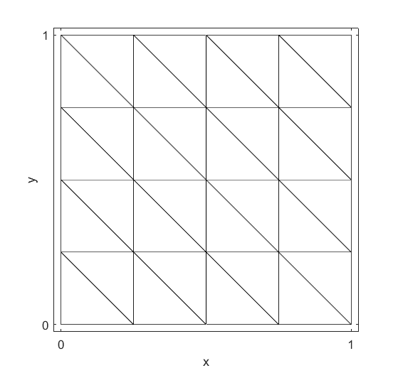
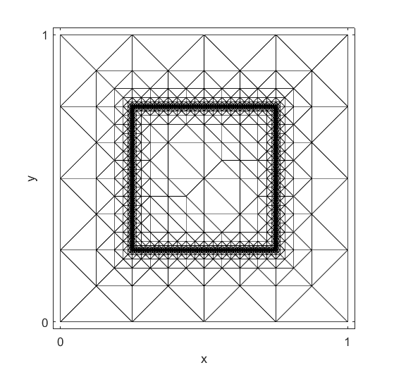
Figure 1: Initial mesh and adaptively refined mesh at level 14 for $\Omega=(0,1)^{2}$ and $\overline{u}_{2D}$.

For a given mesh we compute the approximate solution $\widetilde{u}_{\varrho h}$, the global error

$$\eta:=\|\widetilde{u}_{\varrho h}-\overline{u}\|_{L^{2}(\Omega)},$$

and the local error indicators

$$\eta_{\ell}:=\|\widetilde{u}_{\varrho h}-\overline{u}\|_{L^{2}(\tau_{\ell})},\quad\eta^{2}=\sum\limits_{\ell=1}^{N}\eta_{\ell}^{2}.$$

We mark all elements $\tau_{\ell}$ when

$$\eta_{\ell}>\theta\max\limits_{\ell=1,\ldots,N}\eta_{\ell}$$

is satisfied, with $\theta=0.5$. After $14$ refinement steps we obtain the mesh as shown in Fig. 1 with $1.310.444$ finite elements and $655.215$ degrees of freedom. According to the final error estimate (4.13) we expect a linear order of convergence. The numerical results are shown in Fig. 2 where in addition to the present approach we also present the convergence results when considering energy regularization [18] with the optimal choice $\varrho=h^{2}$, and the regularization in $L^{2}(\Omega)$ with $\varrho=h^{4}$, see [16]. As expected, we observe a linear order of convergence when using the variable energy regularization in the adaptive version described above, while both the energy regularization and the regularization in $L^{2}(\Omega)$ almost coincide with half the order of convergence. For a comparison of the different approaches, see also the computed states as shown in Fig. 3.

Figure 2: Convergence plots for $\overline{u}_{2D}$ choosing $\varrho=h^{4}$ for the $L^{2}(\Omega)$ regularization, $\varrho=h^{2}$ for the energy regularization, and $\varrho(x)=h_{\ell}^{2}$ for $x\in\tau_{\ell}$ for the diffusion regularization.

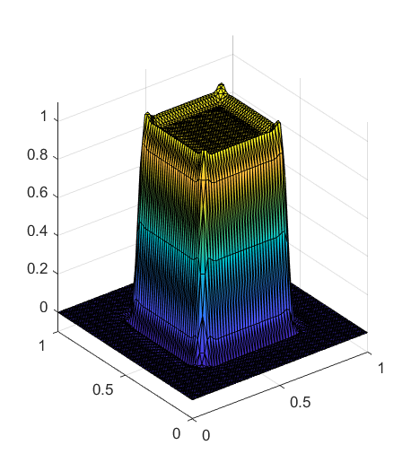
(a) $L^{2}(\Omega)$ regularization

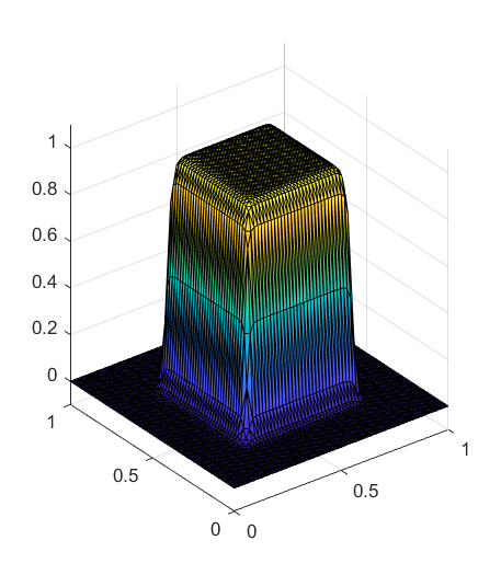
(b) Energy regularization

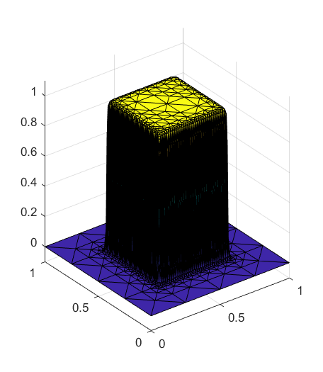
(c) Diffusion regularization

Figure 3: Solution $\widetilde{u}_{\varrho h}$ for the three different regularization approaches, with 8192 finite elements (level 4) using a uniform refinement strategy for $L^{2}(\Omega)$ and energy regularization, and with 4972 finite elements (level 6) for an adaptive refinement for the diffusion regularization.

Next we consider the three-dimensional domain $\Omega=(0,1)^{3}$, and the target function

$$\overline{u}_{3D}(x)=\begin{cases}1&\mbox{for}\;x\in(0.25,0.75)^{3},\\ 0&\mbox{else}.\end{cases}$$

As shown in Fig. 4 we still observe a $h^{1/2}$ convergence for a uniform refinement in the case of both the $L^{2}(\Omega)$ and energy regularizations, but a $h^{3/4}$ convergence for the adaptive diffusion approach, where $h=N^{-1/3}$.

Figure 4: Convergence plots for $\overline{u}_{3D}$ choosing $\varrho=h^{4}$ for the $L^{2}(\Omega)$ regularization, $\varrho=h^{2}$ for the energy regularization, and $\varrho(x)=h_{\ell}^{2}$ for $x\in\tau_{\ell}$ for the diffusion regularization.

To explain the different convergence behaviour for the adaptive refinement in two and three space dimensions, we first consider the 2D case for the example $\overline{u}_{2D}\in H^{1/2-\varepsilon}(\Omega)$, $\varepsilon>0$ for a uniform refinement of the triangulation with $N$ triangles (see Fig. 1 (left)). Let further $m$ denote approximately the number of elements in each row/column of the mesh grid, i.e., $N\sim m\cdot m=m^{2}$. Due to the regularity of $\overline{u}_{2D}$, the optimal order of convergence is de facto $1/2$. Thus, refining all of the $N$ elements uniformly, will lead to a an error reduction of order $h^{1/2}$, as observed. Now we aim for an adaptive refinement. Since for the particular test example the singularity of $\overline{u}_{2D}$ is only along the boundary of the square $(0.25,0.75)^{2}$, it is sufficient (after an initializing phase), to refine only ${\mathcal{O}}(m)={\mathcal{O}}(\sqrt{N})$ elements in the neighborhood of this boundary in order to have the optimal rate of $1/2$. Note, that for a uniform refinement, the number of elements would grow by a factor of 4 in each step, for the adaptive scheme, we only refine ${\mathcal{O}}(m)={\mathcal{O}}(\sqrt{N})$ elements in the neighborhood of the discontinuity. Therefore, the number of elements only grows by a factor of 2. Hence, if we adaptively refine ${\mathcal{O}}(N)$ elements, we can expect an error reduction of order $h$, which is exactly what we see in the numerical example as given in Fig. 2.

Now let us look at the 3D case. Here again counting the elements along each edge, denoted by $m$, we get the relation $N\sim m^{3}$. For a uniform refinement we get a convergence rate $h^{1/2}$. In order to get the same rate with an adaptive scheme, we need to refine at least the elements in the neighborhood of the boundary of the cube $[0.25,0.75]^{3}$, where $\overline{u}_{3D}$ jumps. Each side of the cube consists of approximately ${\mathcal{O}}(m^{2})$ elements. So the whole boundary of the interior cube has approximately ${\mathcal{O}}(m^{2})={\mathcal{O}}(N^{2/3})$ neighboring elements. So, refining $O(N^{2/3})$ elements adaptively gives a rate of $1/2$. Hence, if we refine ${\mathcal{O}}(N)$ elements adaptively, we might expect an error reduction of order $h^{3/2\cdot 1/2}=h^{3/4}$, which is exactly what we observe in Fig. 4.

Finally we consider the one-dimensional domain $\Omega=(0,1)$ and the target

$$\overline{u}_{1D}(x)=\begin{cases}1&\mbox{for}\;x\in(0.25,0.75),\\ 0&\mbox{else}.\end{cases}$$

For $\overline{u}_{1D}\in H^{1/2-\varepsilon}(\Omega)$, $\varepsilon>0$, and for uniformly refining $N$ elements, we will get an error reduction of order $h^{1/2}$. Using an adaptive refinement though, it is enough to refine exactly $4\sim{\mathcal{O}}(\log(N))$ elements in each step to get the optimal order of $1/2$. Thus we can expect exponential convergence, which is also what we observe in the numerical example in Fig. 5.

Figure 5: Convergence plots for $\overline{u}_{1D}$ choosing $\varrho=h^{4}$ for the $L^{2}(\Omega)$ regularization, $\varrho=h^{2}$ for the energy regularization, and $\varrho(x)=h_{\ell}^{2}$ for $x\in\tau_{\ell}$ for the diffusion regularization.

5.2 Control recovering

Once we have computed an approximation $\widetilde{u}_{\varrho h}$ of the state $u_{\varrho}$, we can easily recover the corresponding control via postprocessing. Using $A=-\Delta:H^{1}_{0}(\Omega)\to H^{-1}(\Omega)$ we can write the state equation (1.2) as $A^{-1}z_{\varrho}=u_{\varrho}$, i.e., $z_{\varrho}\in H^{-1}(\Omega)$ solves the variational formulation

$$\langle A^{-1}z_{\varrho},\psi\rangle_{\Omega}=\langle u_{\varrho},\psi\rangle_{\Omega}\quad\mbox{for all}\;\psi\in H^{-1}(\Omega).$$

In addition to the finite element space $V_{h}\subset H^{1}_{0}(\Omega)$ of piecewise linear and continuous basis functions, we now define the ansatz space $Z_{H}=S_{H}^{0}(\Omega)=\text{span}\{\psi_{\ell}\}_{\ell=1}^{N_{H}}$ of piecewise constant basis functions which are defined with respect to some mesh of mesh size $H\sim h$. Hence we may determine $\widetilde{z}_{\varrho H}\in Z_{H}$ as the unique solution of the Galerkin variational formulation

$$\langle A^{-1}z_{\varrho H},\psi_{H}\rangle_{\Omega}=\langle\widetilde{u}_{\varrho h},\psi_{H}\rangle_{\Omega}\quad\mbox{for all}\;\psi_{H}\in Z_{H}.$$

While we can derive related error estimates using standard arguments, in general we are not able to evaluate the inverse operator $A^{-1}$. Hence we need to introduce a suitable approxiation as follows: For any $z\in H^{-1}(\Omega)$ we define $p_{z}\in H^{1}_{0}(\Omega)$ as the unique solution of the variational formulation

$$\langle Ap_{z},q\rangle_{\Omega}=\langle\nabla p,\nabla q\rangle_{L^{2}(\Omega)}=\langle z,q\rangle_{\Omega}\quad\mbox{for all}\;q\in H^{1}_{0}(\Omega).$$

In addition we determine an approximate solution $p_{zh}\in V_{h}$ such that

$$\langle\nabla p_{zh},\nabla q_{h}\rangle_{L^{2}(\Omega)}=\langle z,q_{h}\rangle_{\Omega}\quad\mbox{for all}\;q_{h}\in V_{h},$$

which defines an approximation $\widetilde{A}^{-1}z:=p_{zh}$ of $p_{z}=A^{-1}z$. Hence we finally consider the variational formulation to find $\widehat{z}_{\varrho H}\in Z_{H}$ such that

$$\langle\widetilde{A}^{-1}\widehat{z}_{\varrho H},\psi_{H}\rangle_{\Omega}=\langle\widetilde{u}_{\varrho h},\psi_{H}\rangle_{\Omega}\quad\mbox{for all}\;\psi_{H}\in Z_{H}.$$

Unique solvability follows when $\widetilde{A}^{-1}$ is discrete elliptic for all $\psi_{H}\in Z_{H}$ which can be ensured for an appropriate choice of the finite element spaces $Z_{H}$ and $V_{h}$ where the latter has to be defined on a sufficiently refined mesh than $Z_{H}$. From a practical point of view, one additional refinement is sufficient. Note that the above perturbed variational problem can be written as a mixed variational formulation to find $(\widehat{z}_{\varrho H},p_{\widehat{z}_{\varrho H}h})\in Z_{H}\times V_{h}$ such that

$$\langle p_{\widehat{z}_{\varrho H}h},\psi_{H}\rangle_{L^{2}(\Omega)}=\langle\widetilde{u}_{\varrho h},\psi_{H}\rangle_{L^{2}(\Omega)},\quad\langle\nabla p_{\widehat{z}_{\varrho H}h},\nabla q_{h}\rangle_{L^{2}(\Omega)}=\langle\widehat{z}_{\varrho H},q_{h}\rangle_{L^{2}(\Omega)}$$

is satisfied for all $(\psi_{H},q_{h})\in Z_{H}\times V_{h}$. Related error estimates rely on the use of the Strang lemma. A more detailed numerical analysis of the approach was already given in [9]. Using the fe-isomorphism $\mathbb{R}^{M}\ni\textbf{u}_{\varrho h}\leftrightarrow\widetilde{u}_{\varrho h}\in V_{h}$, we can reconstruct the control $\mathbb{R}^{N_{H}}\ni\textbf{z}_{\varrho H}\leftrightarrow\widehat{z}_{\varrho H}\in Z_{H}$ by solving

$$\begin{pmatrix}K_{h}&-\hat{M}_{h}^{\top}\\ \hat{M}_{h}&0\end{pmatrix}\begin{pmatrix}\textbf{p}_{h}\\ \textbf{z}_{\varrho H}\end{pmatrix}=\begin{pmatrix}\textbf{0}_{h}\\ \hat{M}_{h}\textbf{u}_{\varrho h}\end{pmatrix}$$

where the stiffness and mass matrices admit the entries

$$K_{h}[i,j]=\int_{\Omega}\nabla\varphi_{j}(x)\cdot\nabla\varphi_{i}(x)\,dx\quad\text{and}\quad\hat{M}_{h}[\ell,j]=\int_{\Omega}\varphi_{j}(x)\psi_{\ell}(x)\,dx$$ (5.1)

for $i,j=1,\ldots,M$ and $\ell=1,\ldots,N_{H}$. To obtain stability, the coarse mesh of the control is chosen such that $h=H/4$. The reconstructed controls for the target $\overline{u}_{2D}$ for both a uniform refinement with $N_{H}=2048$ elements and an adaptive refinement with $N_{H}=544$ elements are depicted in Figure 6.

(a) Uniform $N=2048$

(b) Adaptive $N=544$

Figure 6: Reconstructed controls $\hat{z}_{\varrho H}\in Z_{H}$ for the target $\overline{u}_{2D}$ for a uniform and an adaptive refinement.

5.3 Solver studies

While all the numerical results presented in the previous subsection were computed using Matlab with a sparse direct solver, we finally discuss the use of preconditioned iterative solution strategies which are robust with respect to the regularization parameter function $\varrho(x)$. Here we will restrict our considerations to the three-dimensional case with the target $\overline{u}_{3D}$.

We first consider the preconditioned conjugate gradient (PCG) solver applied to the Schur complement equation (4.17) with a proper preconditioner. When performing a uniform refinement, the diffusion coefficients (the inverse of the regularization parameters) are constant on all elements, and we may replace $\varrho(x)$ by $h^{2}$ with $h$ being the global mesh size. Therefore, the Schur complement is simplified as $M_{h}+K_{h}K_{\varrho h}^{-1}K_{h}=M_{h}+\varrho K_{h}K_{h}^{-1}K_{h}=M_{h}+h^{2}K_{h}$. Robust preconditioners for such a Schur complement have been studied in our previous work [17], and the spectral equivalence of this Schur complement to the mass matrix was analyzed in our recent work [16]. Since, in this case, the Schur complement $M_{h}+\varrho K_{h}K_{h}^{-1}K_{h}=M_{h}+h^{2}K_{h}$ is spectrally equivalent to the mass matrix $M_{h}$, we can use a simple diagonal approximation to the mass matrix such as $\textup{diag}[M_{h}]$ or $\textup{lump}[M_{h}]$ as cheap preconditioners for the Schur complement. In the case of an adaptive refinement, both the local mesh refinement and the use of varying diffusion coefficients $\varrho(x)$, which are piecewise constant, play a decisive role in developing robust Schur complement preconditioners with respect to the mesh size and diffusion coefficient jumps. Indeed, the following lemma states that the lumped mass matrix $\textup{lump}[M_{h}]$ is spectrally equivalent to the Schur complement $S_{h}=M_{h}+K_{h}K_{\varrho h}^{-1}K_{h}$.

Lemma 2.

Let us again assume that the computational domain $\Omega\subset\mathbb{R}^{n}$ is decomposed into $N$ shape-regular finite elements $\tau_{\ell}$, $\ell=1,\ldots,N$, and the finite element space $V_{h}=\mbox{span}\{\varphi_{k}\}_{k=1}^{M}\subset H^{1}_{0}(\Omega)$ is spanned by continuous, piecewise linear basis functions. Then the spectral equivalence inequalities

$$c_{1}\,\textup{lump}[M_{h}]\leq M_{h}\leq M_{h}+K_{h}K_{\varrho h}^{-1}K_{h}\leq(1+c_{\text{\tiny inv}}^{2})M_{h}\leq c_{2}\,\textup{lump}[M_{h}]$$ (5.2)

hold, where $c_{1}=1/(n+2)$, $c_{2}=1+c_{\text{\tiny inv}}^{2}$, and $c_{\text{\tiny inv}}$ is nothing but the constant from the local inverse inequalities

$$\|\nabla u_{h}\|_{L^{2}(\tau_{\ell})}\leq c_{\text{\tiny inv}}\,h_{\ell}^{-1}\,\|u_{h}\|_{L^{2}(\tau_{\ell})}\quad\mbox{for all}\;u_{h}\in V_{h},\;\ell=1,2,\ldots,N.$$ (5.3)

We note that $c_{\text{\tiny inv}}$ is a generic positive constant that can be computed from the shape-regularity parameters.

Proof.

It remains to estimate $K_{h}K_{\varrho h}^{-1}K_{h}$ from above by the mass matrix $M_{h}$ in the spectral sense. Using Cauchy’s inequality, (4.1), and the inverse inequalities (5.3), we get the estimate

$$(K_{h}K_{\varrho h}^{-1}K_{h}\underline{u},\underline{u}) = \sup_{\underline{q}\in\mathbb{R}^{M}}\frac{(K_{h}\underline{u},\underline{q})^{2}}{(K_{\varrho h}\underline{q},\underline{q})}$$

$$= \sup_{q_{h}\in V_{h}}\frac{[\int_{\Omega}\varrho^{1/2}\nabla u_{h}\cdot\varrho^{-1/2}\nabla q_{h}\,dx]^{2}}{\int_{\Omega}\varrho^{-1}\nabla q_{h}\cdot\nabla q_{h}\,dx}$$

$$\leq \sup_{q_{h}\in V_{h}}\frac{\|\varrho^{1/2}\nabla u_{h}\|_{L^{2}(\Omega)}^{2}\,\|\varrho^{-1/2}\nabla q_{h}\|_{L^{2}(\Omega)}^{2}}{\|\varrho^{-1/2}\nabla q_{h}\|_{L^{2}(\Omega)}^{2}}$$

$$= \|\varrho^{1/2}\nabla u_{h}\|_{L^{2}(\Omega)}^{2}=\int_{\Omega}\varrho\,\nabla u_{h}\cdot\nabla u_{h}\,dx$$

$$= \sum_{\ell=1}^{N}\int_{\tau_{\ell}}h_{\ell}^{2}\,\nabla u_{h}\cdot\nabla u_{h}\,dx=\sum_{\ell=1}^{N}h_{\ell}^{2}\,\|\nabla u_{h}\|_{L^{2}(\tau_{\ell})}^{2}$$

$$\leq \sum_{\ell=1}^{N}h_{\ell}^{2}c_{\text{\tiny inv}}^{2}h_{\ell}^{-2}\,\|u_{h}\|_{L^{2}(\tau_{\ell})}^{2}=c_{\text{\tiny inv}}^{2}(M_{h}\underline{u},\underline{u})$$

for all nodal vectors $\underline{u}\in\mathbb{R}^{M}$, where $u_{h}\in V_{h}$ is the associated finite element function. The spectral equivalence inequalities

$$(1/(n+2))\,\textup{lump}[M_{h}]\leq M_{h}\leq\textup{lump}[M_{h}]$$ (5.4)

complete the proof. The spectral equivalence inequalities (5.4) can easily be proven by the element matrix representation. ∎

We note that $\textup{lump}[M_{h}]$ can be replaced by $\textup{diag}[M_{h}]$, i.e., $\textup{diag}[M_{h}]$ is also spectrally equivalent to $S_{h}$. The robustness with respect to the minimal and maximal local mesh size ($h_{\min}$ and $h_{\max}$) is numerically confirmed by the constant iteration numbers of the PCG method preconditioned by the lumped mass matrix (Its (PCG)) on the adaptive refinements in Table 1, in comparison with the increasing conjugate gradient (CG) iteration numbers without using the preconditioner (Its (CG)). Note that we solve the Schur complement equation (4.17) until the relative preconditioned residual error is reduced by a factor $10^{6}$. For the inverse operation of $K_{\varrho h}^{-1}$ applied to a vector $\underline{v}$ within the PCG iteration, we have used the classical Ruge–Stüben algebraic multigrid (AMG) [22] preconditioned CG method to solve $K_{\varrho h}\underline{w}=\underline{v}$ until the relative preconditioned residual error reaches $10^{-12}$ in order to perform a sufficiently accurate multiplication with the Schur complement. Alternatively, one can here use a sparse factorization in a preprocessing step.

Level	#Dofs	$h_{\min}$	$h_{\max}$	$\|\widetilde{u}_{\varrho h}-\overline{u}\|_{L^{2}(\Omega)}$	Its (PCG)	Its (CG)
$L_{1}$	$125$	$2^{-2}$	$2^{-2}$	$3.01923$e$-1$	$7$	$8$
$L_{2}$	$223$	$2^{-3}$	$2^{-2}$	$2.55302$e$-1$	$18$	$22$
$L_{3}$	$1,059$	$2^{-4}$	$2^{-2}$	$1.79986$e$-1$	$23$	$52$
$L_{4}$	$4,728$	$2^{-5}$	$2^{-2}$	$1.26353$e$-1$	$26$	$127$
$L_{5}$	$18,827$	$2^{-6}$	$2^{-2}$	$8.84306$e$-2$	$25$	$317$
$L_{6}$	$75,603$	$2^{-7}$	$2^{-2}$	$6.21010$e$-2$	$24$	$829$
$L_{7}$	$303,782$	$2^{-8}$	$2^{-2}$	$4.37439$e$-2$	$23$	$2,103$
$L_{8}$	$1,218,846$	$2^{-9}$	$2^{-2}$	$3.08691$e$-2$	$23$	$5,219$
$L_{9}$	$4,884,317$	$2^{-10}$	$2^{-2}$	$2.18069$e$-2$	$19$	$>10,000$
$L_{10}$	$19,553,202$	$2^{-11}$	$2^{-2}$	$1.54097$e$-2$	$17$	$>20,000$
$L_{11}$	$78,277,988$	$2^{-12}$	$2^{-2}$	$1.08918$e$-2$	$15$	$>40,000$

Table 1: Comparison of the PCG (Its (PCG)) and CG iterations (Its (CG)) for the Schur complement equation (4.17) on the adaptive refinements.

Furthermore, we provide some numerical results concerning robust solvers for the coupled optimality system (4.16):

$$\begin{bmatrix}K_{\varrho h}&K_{h}\\ -K_{h}&M_{h}\end{bmatrix}\begin{bmatrix}\underline{p}\\ \underline{u}\end{bmatrix}=\begin{bmatrix}\underline{0}\\ \underline{f}\end{bmatrix}.$$ (5.5)

Since the system matrix is non-symmetric and positive definite, we apply the GMRES method with the following proposed block diagonal preconditioner:

$${\mathcal{P}}_{h}=\begin{bmatrix}\widehat{K}_{\varrho h}&0\\ 0&\textup{lump}[M_{h}]\end{bmatrix}.$$

The number of GMRES iterations (Its) using such a preconditioner are given in Table 2. We solve the system until the relative preconditioned residual error is reduced by a factor $10^{6}$. In the preconditioner ${\mathcal{P}}_{h}$, we have utilized the Ruge–Stüben AMG preconditioner $\widehat{K}_{\varrho h}$ for $K_{\varrho h}$, whereas the lumped mass matrix $\textup{lump}[M_{h}]$ has been used as preconditioner for the Schur complement. We observe almost constant iteration numbers of the GMRES method preconditioned by ${\mathcal{P}}_{h}$ on the uniform refinement as well as on the adaptive refinements as given in Table 2. We only see slightly higher iteration numbers on the adaptive meshes than on the uniform ones.

Level	Adaptive			Uniform
	#Dofs	$\|\widetilde{u}_{\varrho h}-\overline{u}\|_{L^{2}(\Omega)}$	Its	#Dofs	$\|\widetilde{u}_{\varrho h}-\overline{u}\|_{L^{2}(\Omega)}$	Its
$L_{1}$	$250$	$3.01923$e$-1$	$14$	$250$	$3.01923$e$-1$	$14$
$L_{2}$	$446$	$2.55302$e$-1$	$33$	$1,458$	$2.26341$e$-1$	$28$
$L_{3}$	$2,118$	$1.79985$e$-1$	$40$	$9,826$	$1.61850$e$-1$	$36$
$L_{4}$	$9,456$	$1.26356$e$-1$	$46$	$71,874$	$1.14659$e$-1$	$36$
$L_{5}$	$37,656$	$8.84293$e$-2$	$48$	$549,250$	$8.10582$e$-2$	$34$
$L_{6}$	$151,212$	$6.20997$e$-2$	$47$	$4,293,378$	$5.72923$e$-2$	$32$
$L_{7}$	$607,586$	$4.37450$e$-2$	$46$	$33,949,186$	$4.04944$e$-2$	$30$
$L_{8}$	$2,437,880$	$3.08701$e$-2$	$44$	$270,011,394$	$2.86176$e$-2$	$28$
$L_{9}$	$9,769,496$	$2.18075$e$-2$	$44$
$L_{10}$	$39,108,934$	$1.54100$e$-2$	$42$
$L_{11}$	$156,568,020$	$1.08922$e$-2$	$42$

Table 2: Comparison of the preconditioned GMRES solver on both the adaptive and uniform refinements.

On the other hand, we may reformulate the coupled system (5.5) in the following equivalent form

$$\begin{bmatrix}K_{\varrho h}&K_{h}\\ K_{h}&-M_{h}\end{bmatrix}\begin{bmatrix}\underline{p}\\ \underline{u}\end{bmatrix}=\begin{bmatrix}\underline{0}\\ -\underline{f}\end{bmatrix}.$$ (5.6)

When applying the Bramble–Pasciak transformation

$$\mathcal{T}_{h}=\begin{bmatrix}K_{\varrho h}C_{h}^{-1}-I_{h}&0\\ K_{h}C_{h}^{-1}&-I_{h}\\ \end{bmatrix}$$

to the symmetric but indefinite system (5.6), this leads to the equivalent system

$$\mathcal{K}_{h}\begin{bmatrix}\underline{p}\\ \underline{u}\end{bmatrix}=\begin{bmatrix}\underline{0}\\ \underline{f}\end{bmatrix}\equiv\mathcal{T}_{h}\begin{bmatrix}\underline{0}\\ -\underline{f}\end{bmatrix},$$

with the symmetric and positive definite system matrix

$$\mathcal{K}_{h} =\begin{bmatrix}K_{\varrho h}C_{h}^{-1}-I_{h}&0\\ K_{h}C_{h}^{-1}&-I_{h}\\ \end{bmatrix}\begin{bmatrix}K_{\varrho h}&K_{h}\\ K_{h}&-M_{h}\end{bmatrix}$$

$$=\begin{bmatrix}(K_{\varrho h}-C_{h})C_{h}^{-1}K_{\varrho h}&(K_{\varrho h}-C_{h})C_{h}^{-1}K_{h}\\ K_{h}C_{h}^{-1}(K_{\varrho h}-C_{h})&K_{h}C_{h}^{-1}K_{h}+M_{h}\\ \end{bmatrix}.$$

Here, $I_{h}$ denotes the identity, and $C_{h}$ is some symmetric and positive definite (spd) matrix that is assumed to be spectrally equivalent to the matrix $K_{\varrho h}$, and less than $K_{\varrho h}$, i.e., $C_{h}<K_{\varrho h}$. In particular, we can again take the classical spd Ruge–Stüben AMG preconditioner $\widehat{K}_{\varrho h}=\delta K_{\varrho h}(I_{h}-N_{\varrho h}^{j})^{-1}$ with a proper scaling $\delta>0$ as $C_{h}$, where $N_{\varrho h}$ denotes the AMG iteration matrix, and $j$ the number of AMG cycles; see, e.g., [26]. In our numerical experiments, we have chosen $\delta=0.5$, and we use the AMG V-cycle with $2$ forward Gauss-Seidel pre-smoothing steps and $2$ backward Gauss-Seidel post-smoothing steps at all levels, where $j$ is equal to $8$ and $12$ for uniform and adaptive refinements, respectively. Now using $C_{h}=\widehat{K}_{\varrho h}$ and the lumped mass matrix $\textup{lump}[M_{h}]$ as preconditioner for the Schur complement $M_{h}+K_{h}K_{\varrho h}^{-1}K_{h}$, we arrive at the following (inexact) BP preconditioner:

$${\mathcal{P}}_{h}=\begin{bmatrix}K_{\varrho h}-C_{h}&0\\ 0&\textup{lump}[M_{h}]\end{bmatrix}.$$

Details on the BP-CG can be found in the original paper [3]; see also [27] for improved convergence rate estimates. The number of BP-CG iterations (Its) using the preconditioner ${\mathcal{P}}_{h}$ are provided in Table 3. The solver stops the iteration when the relative preconditioned residual error is reduced by a factor $10^{6}$. From the constant PB-CG iteration numbers on both the uniform and adaptive mesh refinements, we observe the robustness of the proposed preconditioner for the coupled optimality system.

Level	Adaptive			Uniform
	#Dofs	$\|\widetilde{u}_{\varrho h}-\overline{u}\|_{L^{2}(\Omega)}$	Its	#Dofs	$\|\widetilde{u}_{\varrho h}-\overline{u}\|_{L^{2}(\Omega)}$	Its
$L_{1}$	$250$	$3.01923$e$-1$	$13$	$250$	$3.01923$e$-1$	$13$
$L_{2}$	$446$	$2.55302$e$-1$	$32$	$1,458$	$2.26348$e$-1$	$25$
$L_{3}$	$2,118$	$1.79986$e$-1$	$34$	$9,826$	$1.61863$e$-1$	$30$
$L_{4}$	$9,456$	$1.26353$e$-1$	$38$	$71,874$	$1.14657$e$-1$	$31$
$L_{5}$	$37,654$	$8.84307$e$-2$	$39$	$549,250$	$8.10658$e$-2$	$25$
$L_{6}$	$151,206$	$6.21010$e$-2$	$38$	$4,293,378$	$5.73048$e$-2$	$24$
$L_{7}$	$607,558$	$4.37438$e$-2$	$36$	$33,949,186$	$4.05125$e$-2$	$23$
$L_{8}$	$2,437,674$	$3.08690$e$-2$	$35$	$270,011,394$	$2.86430$e$-2$	$23$
$L_{9}$	$9,768,526$	$2.18067$e$-2$	$33$
$L_{10}$	$39,105,552$	$1.54096$e$-2$	$34$
$L_{11}$	$156,550,890$	$1.089170$$-2$	$30$

Table 3: Comparison of the preconditioned PB-CG solver on both the adaptive and uniform refinements.

Now we can use the preconditioned PB-CG solver in a nested iteration process that interpolates the iterative approximation from the coarser mesh in order to obtain a good initial guess; see, e.g., [10]. Table 4 shows that we can obtain approximate solutions $\widetilde{u}_{\varrho h}$, which differ from the desired state $\overline{u}$ in the order of the discretization error, with considerable less iterations that are pretty constant across the levels; cf. also with Table 3.

Level	Adaptive			Uniform
	#Dofs	$\|\widetilde{u}_{\varrho h}-\overline{u}\|_{L^{2}(\Omega)}$	Its	#Dofs	$\|\widetilde{u}_{\varrho h}-\overline{u}\|_{L^{2}(\Omega)}$	Its
$L_{1}$	$250$	$3.01923$e$-1$	$13$	$250$	$3.01923$e$-1$	$13$
$L_{2}$	$446$	$2.55278$e$-1$	$12$	$1,458$	$2.26412$e$-1$	$10$
$L_{3}$	$2,118$	$1.80027$e$-1$	$13$	$9,826$	$1.61959$e$-1$	$12$
$L_{4}$	$9,458$	$1.26535$e$-1$	$16$	$71,874$	$1.14724$e$-1$	$12$
$L_{5}$	$37,696$	$8.84904$e$-2$	$16$	$549,250$	$8.11476$e$-2$	$11$
$L_{6}$	$151,220$	$6.21325$e$-2$	$16$	$4,293,378$	$5.73597$e$-2$	$11$
$L_{7}$	$607,170$	$4.37623$e$-2$	$16$	$33,949,186$	$4.05516$e$-2$	$11$
$L_{8}$	$2,435,524$	$3.08822$e$-2$	$16$	$270,011,394$	$2.86695$e$-2$	$11$
$L_{9}$	$9,758,590$	$2.18163$e$-2$	$16$
$L_{10}$	$39,065,548$	$1.54165$e$-2$	$16$
$L_{11}$	$156,371,118$	$1.089660$$-2$	$16$

Table 4: Comparison of the preconditioned PB-CG solver on both the adaptive and uniform refinements using nested iteration, where the stopping criterio for the nested iteration is: the relative preconditioned residual error of the full system (including both state and adjoint states) is smaller than $\alpha[n_{l}/n_{l-1}]^{-\frac{\beta}{3}}$, $l=2,3,...$, $\beta=0.5$ (uniform), $\beta=0.75$ (adaptive), and $\alpha=0.025$.

6 Conclusion and outlook

We have studied finite element discretizations of the reduced optimality system for the standard distributed space-tracking elliptic optimal control problem, but using a new variable energy regularization technique. It has been shown that the choice of the local mesh-size squared as local regularization parameter $\varrho(x)$ leads to optimal rates of convergence of the computed finite element state $\widetilde{u}_{\varrho h}$ to the prescribed target $\overline{u}$ in the $L^{2}$ norm. In particular, this approach allows us to adapt the local regularization parameter to the local mesh-size when using an adaptive mesh refinement, where the adaptivity is driven by the localization of the $L^{2}$ norm of the error between $\overline{u}$ and $\widetilde{u}_{\varrho h}$ as computable local error indicator. Numerical studies made for discontinuous targets in one, two and three space dimensions illustrate that these simple adaptive schemes show a significantly better performance than the uniform refinement. The control can easily be recovered from the computed state in a postprocessing procedure. We have also proposed iterative solvers for the finite element equations corresponding to the reduced optimality system. The numerical studies have shown that these solvers are robust and efficient at the same time. This behavior is based on the fact that the mass matrix $M_{h}$, and, therefore, also the lumped mass matrix $\text{lump}[M_{h}]$ are spectrally equivalent to the Schur complement $K_{h}K_{\varrho h}^{-1}K_{h}+M_{h}$, and can be used as robust preconditioners in the preconditioned BP-CG, MINRES, or GMRES solvers. Obviously, the classical plain Ruge–Stüben AMG preconditioner is doing this job for $K_{\varrho h}$. Here we may develop more efficient and robust preconditioners that are especially adapted to the diffusion coefficient $\varrho(x)$ that changes from element to element according to the mesh-sizes. In a possibly adaptive, multilevel setting, the nested iteration technique can be used to compute state approximations which differ from the desired state in the order of the discretization error in asymptotically optimal complexity. The computation of the control can be integrated in the nested iteration process that can then be stopped if the cost of the computed control exceeds some threshold or the required approximation of the desired state is reached. Moreover, the parallelization of such iterative solution strategies should be implemented in order to solve really large-scale systems in three space dimensions.

Finally, the variable energy regularization and the robust solvers for the corresponding linear system of algebraic equations can be extended to optimal control problems with state or control constraints; see [9] for the case of a constant regularization parameter. Furthermore, the results can be generalized to other state equations like elasticity, Maxwell, and Stokes equations, but also to time-dependent problems such as parabolic and hyperbolic initial boundary value problems [18, 20].

Declarations

Conflict of interest: The authors declared that they have no conflict of interest.
Data availability: Data will be made available on request.

References

- [1] V. Albani, A. De Cezaro, and J. P. Zubelli. On the choice of the Tikhonov regularization parameter and the discretization level: a discrepancy-based strategy. Inverse Probl. Imaging, 10(1):1–25, 2016.
- [2] A. Borzì and V. Schulz. Computational optimization of systems governed by partial differential equations, volume 8 of Computational Science & Engineering. Society for Industrial and Applied Mathematics (SIAM), Philadelphia, PA, 2012.
- [3] J. H. Bramble and J. E. Pasciak. A preconditioning technique for indefinite systems resulting from mixed approximations of elliptic problems. Math. Comp., 50(181):1–17, 1988.
- [4] K. Bredies, Y. Dong, and M. Hintermüller. Spatially dependent regularization parameter selection in total generalized variation models for image restoration. Int. J. Comput. Math., 90:109–123, 2013.
- [5] S. C. Brenner and L. R. Scott. The mathematical theory of finite element methods, volume 15 of Texts in Applied Mathematics. Springer, New York, third edition, 2008.
- [6] C. Chung, J. De los Reyes, and C. Schönlieb. Learning optimal spatially-dependent regularization parameters in total variation image denoising. Inverse Problems, 33:074005, 2017.
- [7] C. Clason and B. Kaltenbacher. Optimal control and inverse problems. Inverse Problems, 36:060301, 2020.
- [8] H. Engl, M. Hanke, and A. Neubauer. Regularization of Inverse Problems, volume 375 of Mathematics and its Applications. Kluwer, Dordrecht, 1996.
- [9] P. Gangl, R. Löscher, and O. Steinbach. Regularization and finite element error estimates for elliptic distributed optimal control problems with energy regularization and state or control constraints, 2023. arXiv:2306.15316.
- [10] W. Hackbusch. Iterative Solution of Large Sparse Systems of Equations, volume 95 of Applied Mathematical Sciences. Springer, second edition, 2016.
- [11] M. Hintermüller, K. Papafitsoros, C. N. Rautenberg, and H. Sun. Dualization and automatic distributed parameter selection of total generalized variation via bilevel optimization. Numer. Funct. Anal. Optim., 43:887–932, 2022.
- [12] M. Hinze, R. Pinnau, M. Ulbrich, and S. Ulbrich. Optimization with PDE Constraints, volume 23. Springer-Verlag, Berlin, 2009.
- [13] B. Hong, J. Koo, and M. Burger. Adaptive regularization in convex composite optimization for variational imaging problems. In V. Roth and T. Vetter, editors, Pattern Recognition. GCPR 2017, volume 10496 of Lecture Notes in Computer Science, pages 268–280. Springer, Cham, 2017.
- [14] V. Isakov. Inverse problems for partial differential equations, volume 127 of Applied Mathematical Sciences. Springer, Cham, third edition, 2017.
- [15] V. John. Finite Element Methods for Incompressible Flow Problems, volume 51 of Springer Series in Computational Mathematics. Springer, 2016.
- [16] U. Langer, R. Löscher, O. Steinbach, and H. Yang. Robust finite element discretization and solvers for distributed elliptic optimal control problems, 2022. arXiv:2207.04664.
- [17] U. Langer, O. Steinbach, and H. Yang. Robust discretization and solvers for elliptic optimal control problems with energy regularization. Comput. Meth. Appl. Math., 22:97–111, 2022.
- [18] U. Langer, O. Steinbach, and H. Yang. Robust space-time finite element error estimates for parabolic distributed optimal control problems with energy regularization, 2022. arXiv:2206.06455.
- [19] J.-L. Lions. Optimal control of systems governed by partial differential equations. Die Grundlehren der mathematischen Wissenschaften, Band 170. Springer-Verlag, New York-Berlin, 1971.
- [20] R. Löscher and O. Steinbach. Space-time finite element methods for distributed optimal control of the wave equation. arXiv:2211.02562v1, 2022.
- [21] M. Neumüller and O. Steinbach. Regularization error estimates for distributed control problems in energy spaces. Math. Methods Appl. Sci., 44:4176–4191, 2021.
- [22] J. W. Ruge and K. Stüben. Algebraic multigrid (AMG). In S. F. McCormick, editor, Multigrid Methods, pages 73–130. Society for Industrial and Applied Mathematics, Philadelphia, 1987.
- [23] T. Schuster, B. Kaltenbacher, B. Hofmann, and K. Kazimierski. Regularization Methods in Banach Spaces, volume 10 of Radon Series on Computational and Applied Mathematics. de Gruyter, Berlin, 2012.
- [24] H. Triebel. Interpolation theory, function spaces, differential operators, volume 18 of North-Holland Mathematical Library. North-Holland Publishing Co., Amsterdam-New York, 1978.
- [25] F. Tröltzsch. Optimal control of partial differential equations, volume 112 of Graduate Studies in Mathematics. American Mathematical Society, Providence, RI, 2010.
- [26] U. Trottenberg, C. Oosterlee, and A. Schüller. Multigrid. Academic Press, London, 2001.
- [27] W. Zulehner. Analysis of iterative methods for saddle point problems: a unified approach. Math. Comp., 71(238):479–505, 2002.