Grid-Free MIMO Beam Alignment through Site-Specific Deep Learning

Abstract

Beam alignment is a critical bottleneck in *mmWave communication. An ideal beam alignment technique should achieve high *BF gain with low latency, scale well to systems with higher carrier frequencies, larger antenna arrays and multiple *UE, and not require hard-to-obtain *CI. These qualities are collectively lacking in existing methods. We depart from the conventional *CB approach where the optimal beam is chosen from quantized codebooks and instead propose a *GF beam alignment method that directly synthesizes the *Tx and *Rx beams from the continuous search space using measurements from a few site-specific probing beams found via a *DL pipeline. In realistic settings, the proposed method achieves a far superior *SNR-latency trade-off compared to the *CB baselines: it aligns near-optimal beams 100x faster or equivalently finds beams with 10-15 dB higher average *SNR in the same number of searches, relative to an exhaustive search over a conventional codebook.

I Introduction

mmWave devices require highly directional BF to compensate for the severe isotropic path loss and to achieve viable signal strength. To reduce the cost and power consumption of a fully digital system, practical mmWave systems often adopt analog beams that concentrate energy in particular directions. On the other hand, the optimal choice of these narrow beams are susceptible to changes in the propagation environment such as blockage and reflection. It is critical for mmWave BS and UE to find good BF directions during initial connection and then track these analog beams as the propagation conditions change, such as when a UE moves and rotates. As future cellular systems move to unlock larger bandwidths at higher carrier frequencies extending to the so-called “sub-THz” bands of up to 300 GHz, devices will adopt ever denser antenna arrays and narrower beams. As a result, beam management – the process of discovering and maintaining good analog BF directions – is a severe challenge that will only worsen as we move towards 6G and beyond.

I-A Background and Related Work

Existing beam management approaches typically assume a “grid-of-beams” or CB framework, where BS and UE adopt codebooks of quantized BF directions. In order to ensure coverage in any site, the quantized beams usually distribute energy uniformly in the angular space, such as by using DFT codebooks. In this context, the problem of beam alignment becomes selecting the optimal beams from the finite codebooks at the BS and potentially at the UE. The most widely adopted method of beam selection is through a search. For instance, 5G NR adopts a beam management framework based on beam sweeping, measurement and reporting [2, 3]. In the downlink, the BS exhaustively searches its codebook by periodically sending beamformed RS called SSB. The UE measures and reports the received signal strength, and the BS then selects the best beam based on the UE’s feedback. The obvious drawback of an exhaustive search is its beam sweeping latency, which grows linearly with the total number of beam pairs. As systems move higher in frequency and adopt narrower beams, the size of the codebook increases accordingly. A THz system may easily adopt tens of thousands of beam pairs, rendering the the exhaustive search infeasible due to the prohibitive beam sweeping latency. A hierarchical search can reduce the latency for a single UE. By sweeping wider beams first and progress to narrower child beams, it iteratively reduces the search space. In the 5G NR framework, the BS can use SSB to sweep the wide beams and use the more flexible CSI-RS for narrow-beam refinement. On the other hand, the radiation patterns of the wide beams need to be carefully designed since the hierarchical search is more prone to search errors caused by noisy measurements and imperfect wide-beam shapes [4, 5].

Another way to reduce the beam sweeping latency is to leverage CI. The optimal beam pair of a link is intuitively a function of the topology of the propagation environment and the locations of the BS and the UE. Such spatial properties can be captured through CI such as sub-6 GHz OOB measurements [6], GNSS coordinates of the UE [7, 8], radar measurements [9, 10], images captured by cameras and 3D point clouds of the environment [11, 12]. By constructing a mapping from the CI to the index of the optimal beam through a lookup table or ML models, the search space can be substantially reduced. However, these CI-based methods are difficult to standardize and are not widely-adopted in practice due to the requirement of additional sensors and the varying hardware capabilities of mmWave devices. They are also not suitable for standalone systems due to the need of a robust feedback link usually occupying a lower frequency band.

Inspired by the success of DL in computer vision and natural language processing, recent works have explored DL in beam management. NN models can extract features from side information such as CI [12, 7, 10, 11] and history measurements [13] to predict the optimal beam. RL approaches have been proposed to learn beam management policies through iterative interactions with the environment [14, 15]. Reviews of beam management solutions based on ML and DL can be found in [16, 17].

I-B Site-specific Adaptation

A promising way to reduce the beam sweeping latency is through site-specific adaptation. In scenarios where the AoA and AoD distributions of the channel paths are highly non-uniform, such as in particular environment topologies and when there are several spatial clusters of UE, some beams in a uniform codebook may never get used. Leveraging this fact, the BS can compute the statistics of the entire codebook after an exhaustive training phase and prioritize the most frequently used beams [18, 19]. By training using explicit CSI [20] or through implicit rewards in a RL framework [21], NN can generate smaller codebooks from scratch that adapt to the environment and strategically direct energy towards the UE. The data-driven approach can also help select analog beams from standard codebooks using sensing measurements by optimizing the mapping function [22] or jointly learning the sensing beams and the mapping function [23].

Compared to CB beam management methods whose BF gain is limited by the resolution of the codebook, a GF approach extends the search space for the optimal beam to the high-dimensional continuous space and can in theory achieve better gain. For instance, MRT is known to be optimal under the unit power constraint and EGT under the unit modulus constraint. However, they require full CSI to compute the BF weights, which is generally unavailable before beam alignment. Furthermore, even with CSI, finding the optimal EGT and EGC beams requires a grid search over possible weights in the MIMO setting and is computationally prohibitive [24]. Recent works have explored directly predicting the hybrid BF weights for the BS without full CSI by learning sensing matrices [25] or a sequence of interactive sensing vectors based on feedback of previous measurements [26].

In our previous work [27], we proposed a CB beam alignment method that uses the measurements of a few site-specific probing beams to predict the index of the optimal Tx narrow beam. However, it benefits significantly from trying a few candidate beams for each UE. As a result, the gain in the beam sweeping overhead diminishes with increasing number of UE. This is a common and important limitation of many existing methods: the hierarchical search requires searching all child beams, many CI-based models require trying the most likely candidates, and active learning-based methods require sweeping a different sequence of sensing beams for each UE. A beam sweeping procedure needs to be repeated for all UE in the cell, each of which may require a different set of beams. Hence the total beam sweeping latency increases linearly with the number of UE, which can be large and unknown in cellular systems. In CB approaches, eventually the entire codebook will need to be searched, a major shortcoming of many of the aforementioned methods.

I-C Contributions

In this work, we propose DL-GF, a one-shot GF beam alignment method based on unsupervised DL. The proposed method learns a small number of probing beams through site-specific training and directly predicts the optimal analog BF vectors without using a quantized codebook. It possesses several qualities of an ideal beam alignment method, many of which are lacking in existing approaches:

• High BF gain beyond standard codebooks. The proposed method synthesizes continuous-valued analog BF weights. With the additional degree of freedom, the synthesized beams can achieve better BF gain compared to choosing optimally from large quantized codebooks.

• Low beam sweeping latency with optimal scaling. With site-specific training, the proposed method requires sweeping just a few probing beam pairs to capture sufficient channel information. Unlike many existing approaches that require sweeping a few candidate beams or child beams for each UE, the proposed method synthesizes the analog beams in one-shot. As a result, the beam sweeping latency does not increase with the number of UE. In our setting, DL-GF reduces the beam sweeping overhead by over 500$\times$ vs. the exhaustive CB method regardless of the number of UE.

• Easy to adopt in cellular standards. The proposed method does not require hard-to-obtain CI such as the location of UE and OOB measurements. Instead, it purely relies on measuring and reporting a few probing beams. The probing beams are also optimized for coverage, allowing the BS to discover new UE.

• Joint Tx-Rx beam alignment. Unlike many existing methods that only consider beam alignment for the BS, the proposed method jointly predicts the analog beam for both the BS and the UE without any additional beam sweeping for the UE. The synthesized Tx and Rx beam pairs are jointly optimized to achieve high BF gain, even when the UE have random orientations.

A preliminary version of this work considers Tx-only beam alignment [1]. This work extends the conference version to consider Tx and Rx joint beam alignment in the MIMO setting, proposes a more sophisticated utility function, and presents much more comprehensive results.

The rest of this article is organized as follows. The system model is described in Section II. The proposed beam alignment approach, the appropriate metrics and the baselines of comparison are explained in Section III. The datasets used are described in Section IV. The simulation results are presented in Section V. We provide the conclusion and final remarks in Section VI.

Notation: The following notations are used in this paper: $|a|$ denotes the magnitude of the scalar $a$, $||\mathbf{A}||_{\mathrm{F}}$ denotes the Frobenius norm, $\mathbf{A}^{\mathrm{real}},\mathbf{A}^{\mathrm{imag}}$ denote the real and imaginary parts of a complex matrix $\mathbf{A}$, $\mathbf{A}^{T}$ denotes the transpose, $\mathbf{A}^{H}$ denotes the conjugate transpose, $\mathrm{diag}(\mathbf{a})$ denotes the diagonal matrix constructed from the vector $\mathbf{a}$, $\mathrm{diag}(\mathbf{A})$ denotes the vector of diagonal elements of the matrix $\mathbf{A}$, $[\mathbf{a}]_{i}$ denotes the $i$th element of the vector $\mathbf{a}$, $\mathbf{a}\otimes\mathbf{b}$ denotes the Kronecker product, $\mathbf{A}\oslash\mathbf{B}$ denotes the element-wise division and $\mathbf{A}^{|\cdot|}$ denotes the element-wise magnitude.

II System Model

A MIMO system is considered where the BS has an array of $N_{\textnormal{T}}$ antennas, the UE has an array of $N_{\textnormal{R}}$ antennas and both perform beam alignment. A geometric channel model with $L$ paths is adopted:

$$\mathbf{H}=\sum_{l=1}^{L}\alpha_{l}e^{j(\theta_{l}-2\pi\tau_{l}B)}\mathbf{a}_{\textnormal{R}}(\omega_{l}^{az},\omega_{l}^{el})\mathbf{a}_{\textnormal{T}}(\phi_{l}^{az},\phi_{l}^{el})^{H},$$ (1)

where $\mathbf{a}_{\textnormal{T}},\mathbf{a}_{\textnormal{R}}$ are the Tx and Rx array response vectors, $\alpha_{l},\theta_{l},\tau_{l}$ are the gain, Doppler shift and delay, $\omega_{l}^{az},\omega_{l}^{el},\phi_{l}^{az},\phi_{l}^{el}$ are the azimuth and elevation AoA and AoD of path $l$. For a UPA with $N_{y}$ and $N_{z}$ antennas in the $y-z$ plane, its array response vector is given by:

$$\mathbf{a}_{y}(\phi^{az},\phi^{el})=\\ \begin{bmatrix}1&e^{j\frac{2\pi}{\lambda}d\sin\phi^{az}\sin\phi^{el}}&\cdots&e^{j(N_{y}-1)\frac{2\pi}{\lambda}d\sin\phi^{az}\sin\phi^{el}}\end{bmatrix}^{T},$$ (2)

$$\mathbf{a}_{z}(\phi^{el})=\begin{bmatrix}1&e^{j\frac{2\pi}{\lambda}d\cos\phi^{el}}&\cdots&e^{j(N_{z}-1)\frac{2\pi}{\lambda}d\cos\phi^{el}}\end{bmatrix}^{T},$$ (3)

$\lambda$ is the carrier wavelength and $d$ is the antenna spacing.

During data transmission in the downlink, if the BS adopts a Tx beam $\mathbf{v}_{\textnormal{T}}\in\mathbbm{C}^{N_{\textnormal{T}}\times 1}$ and transmits a symbol $s$ and the UE adopts a Rx beam $\mathbf{v}_{\textnormal{R}}\in\mathbbm{C}^{N_{\textnormal{R}}\times 1}$, the received signal can be written as

$$y=\sqrt{P_{\textnormal{T}}}\mathbf{v}_{\textnormal{R}}^{H}\mathbf{H}\mathbf{v}_{\textnormal{T}}s+\mathbf{v}_{\textnormal{R}}^{H}\mathbf{n},$$ (4)

where $P_{\textnormal{T}}$ is the Tx power and $\mathbf{n}\sim\mathcal{CN}(0,\sigma^{2}\mathbb{I})$ is a complex AWGN. Assuming unit-power transmitted symbols, the SNR achieved by the beam pair is

$$\textnormal{SNR}=\frac{P_{\textnormal{T}}|\mathbf{v}_{\textnormal{R}}^{H}\mathbf{H}\mathbf{v}_{\textnormal{T}}|^{2}}{\sigma^{2}}.$$ (5)

The BS and the UE are assumed to perform analog BF only. Each device has a single RF chain connected to an array of phase shifters. Hence the BF vectors satisfy the unit-power, constant modulus constraint:

$$|[\mathbf{v}_{\textnormal{T}}]_{i}|=\frac{1}{\sqrt{N_{\textnormal{T}}}},i=1,\dots,N_{\textnormal{T}}\$$ (6)

$$|[\mathbf{v}_{\textnormal{R}}]_{j}|=\frac{1}{\sqrt{N_{\textnormal{R}}}},j=1,\dots,N_{\textnormal{R}}.$$ (7)

The orientation of a UE is modeled with random rotations with respect to the local coordinate system which is attached to and rotates with the UE [28]. Each UE first rotates by the $z$ axis, then by the new $y$ axis, and finally by the new $x$ axis. The angles of the three elemental rotations are modeled as random variables. The AoA of the channel is then adjusted according to the orientation of the UE. A more sophisticated model may consider the shape of the UE and self–blockage of the device, which is left for future work.

III The Proposed Method, Metrics and Baselines

Our objective is to directly predict optimal Tx and Rx beams without searching large codebooks or candidate beams. In our previous work [27], we demonstrated that a NN classifier can accurately select the optimal beam index from a large codebook using measurements of a few learned site-specific probing beams, i.e., each BS learns unique probing beams that are well-suited to its propagation environment. Inspired by this idea, we propose to learn a small number of probing beam pairs at the BS and the UE then use their measurements to synthesize the optimal narrow beam pair from the continuous search space. The BS first sweeps $N_{\mathbf{F}}$ Tx probing beams while the UE measures the received signal power using $N_{\mathbf{W}}$ Rx sensing beams. After the probing-beam sweeping phase, the UE uses the collected measurements as inputs to its beam synthesizer function $f_{\textnormal{R}}$ to generate its Rx beam. The measurements are also fed back to the BS, which uses them as inputs to its own beam synthesizer function $f_{\textnormal{T}}$ to generate the Tx beam.

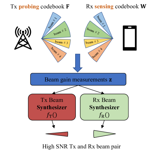
Figure 1: Illustration of the proposed beam alignment procedure based on site-specific probing. The learned probing and sensing beams are implemented in RF and measured through beam sweeping.

The proposed beam alignment procedure is illustrated in Fig. 1. During the first phase of the proposed method, the BS and the UE sweep a small number of probing and sensing beams to capture information about the channel. Let $\mathbf{F}\in\mathbbm{C}^{N_{\textnormal{T}}\times N_{\mathbf{F}}},\mathbf{W}\in\mathbbm{C}^{N_{\textnormal{R}}\times N_{\mathbf{W}}}$ be matrices representing the BS probing and UE sensing beams, whose entries satisfy the constant modulus constraint for analog BF. The BS periodically broadcasts probing symbols $\mathbf{s}_{\textnormal{probe}}$ using beams in $\mathbf{F}$ while each UE measures using the sensing beams in $\mathbf{W}$. Note that all UE in the cell share the same sensing beams. The periodic sweeping of the probing beams is similar to SSB transmission in 5G, which also allows new UE to be discovered and synchronize to the BS. The total number of beams swept does not increase with the number of UE since multiple UE can measure the probing beams using shared time and frequency resources.

After beam sweeping, the composite received signal $\mathbf{Y}\in\mathbbm{C}^{N_{\mathbf{W}}\times N_{\mathbf{F}}}$ consisting of the received signal of all combinations of probing and sensing beams can be written as

$$\mathbf{Y}=\sqrt{P_{\textnormal{T}}}\mathbf{W}^{H}\mathbf{H}\mathbf{F}\mathrm{diag}(\mathbf{s}_{\textnormal{probe}})+\mathbf{W}^{H}\mathbf{N},$$ (8)

where $\mathbf{s}_{\textnormal{probe}}\in\mathbbm{C}^{N_{\textnormal{F}}\times 1}$ is the vector of transmitted probing symbols and $\mathbf{N}\in\mathbbm{C}^{N_{\textnormal{R}}\times N_{\mathbf{F}}}$ is the AWGN measurement noise matrix whose each element has noise power $\sigma_{\textnormal{probe}}^{2}$.

The probing beam pairs will likely have lower gain since there are many fewer of them to cover the angular space. To combat the low SNR during the probing measurement phase, the BS can introduce redundancy in the probing symbols over time or frequency, such as by using a spreading sequence or repeating over subcarriers [2, 29]. This is not too wasteful in the context of analog BF and 5G beam alignment, since a single analog beam can be transmitted at a time (such as for each SSB). A spreading gain of $\beta\geq 1$ is introduced to model the effective SNR of the probing measurements:

$$\textnormal{SNR}_{\textnormal{probe}}=\beta\frac{P_{\textnormal{T}}|\mathbf{w}^{H}\mathbf{H}\mathbf{f}|^{2}}{\sigma^{2}}.$$ (9)

We focus on the special case where $N_{\mathbf{F}}=N_{\mathbf{W}}=N_{\mathrm{probe}}$: the BS sweeps $N_{\mathrm{probe}}$ probing beams while the UE uses a different Rx sensing beam for each Tx probing beam so that the total number of probing beam pairs is $N_{\mathrm{probe}}$. The UE then reports the $N_{\mathrm{probe}}$ received signal power measurements. As a result, the input feature to the beam synthesizer functions is

$$\mathbf{z}=\begin{bmatrix}|[\mathrm{diag}(\mathbf{Y})]_{1}|^{2}&\cdots&|[\mathrm{diag}(\mathbf{Y})]_{N_{\mathrm{probe}}}|^{2}\end{bmatrix}^{T}.$$ (10)

The beam synthesizer functions $f_{\textnormal{T}},f_{\textnormal{R}}$ at the BS and the UE then predict the Tx and Rx beams for data transmission.

In principle, both the measurement and the feedback procedures are flexible and can be design choices. For example, the number of probing and sensing beams can be arbitrary. The UE can measure and feedback all combinations of probing and sensing beams, and the beam synthesizer functions can utilize the full measurement matrix $\mathbf{Y}\in\mathbbm{C}^{N_{\mathbf{W}}\times N_{\mathbf{F}}}$ to generate the BF vectors. The UE may also feedback just $N_{\mathbf{F}}$ measurements corresponding to the strongest sensing beam for each Tx probing beam. The specific design considered in this work is motivated by our wish to reduce the measurement and feedback overhead, i.e., $N_{\mathrm{probe}}\ll N_{\mathbf{F}}N_{\mathbf{W}}$. Furthermore, it is also more compatible with the RS feedback procedure in 5G NR, where the UE beam is transparent to the BS. A comparison of different probing strategies is discussed in Sect. V-C1. However, there is extensive scope for future work exploring other approaches.

III-A Problem Formulation

The parameters of the proposed method include the probing and sensing beams $\mathbf{F},\mathbf{W}$ as well as the beam synthesizers $f_{\textnormal{T}},f_{\textnormal{R}}$, which need to be optimized with respect to a utility function. With the unit modulus constraint of the probing and predicted beam pairs in mind, the optimization problem can be written as:

$$\begin{array}[]{rrcll}\displaystyle\max_{\mathbf{F},\mathbf{W},f_{\textnormal{T}},f_{\textnormal{R}}}&&\mathcal{U}&&\\ \textrm{s.t.}&\mathbf{v}_{\mathrm{T}}&=&f_{\textnormal{T}}(\mathbf{z})&\\ &\mathbf{v}_{\mathrm{R}}&=&f_{\textnormal{R}}(\mathbf{z})&\\ &|[\mathbf{v}_{\mathrm{T}}]_{i}|&=&\frac{1}{\sqrt{N_{\textnormal{T}}}},&\forall i=1,\cdots,N_{\textnormal{T}}\\ &|[\mathbf{v}_{\mathrm{R}}]_{i}|&=&\frac{1}{\sqrt{N_{\textnormal{R}}}},&\forall i=1,\cdots,N_{\textnormal{R}}\\ &|[\mathbf{F}]_{i,j}|&=&\frac{1}{\sqrt{N_{\textnormal{T}}}},&\forall i=1,\cdots,N_{\textnormal{T}},\\ &&&&\forall j=1,\cdots,N_{\mathbf{F}}\\ &|[\mathbf{W}]_{i,j}|&=&\frac{1}{\sqrt{N_{\textnormal{R}}}},&\forall i=1,\cdots,N_{\textnormal{R}},\\ &&&&\forall j=1,\cdots,N_{\mathbf{W}}.\\ \end{array}$$ (11)

There are several considerations when designing the utility function. The beam synthesizer functions should generate beams that tend to maximize the BF gain for each channel realization. The probing and sensing beams in $\mathbf{F}$ and $\mathbf{W}$ serve two important purposes. First, they provide helpful information to the beam synthesizers and thus should capture characteristics of the channel. Second, they should allow the BS to discover new UE during the IA process and thus should satisfy a minimum SNR requirement. Since the optimal BF vectors can be easily computed in closed-form in the simpler MISO or SIMO setting, the synthesized beams can be optimized to resemble the optimal EGT or EGC beams by minimizing a supervised loss function such as the MSE in [20]. However, finding the EGT and EGC beam pairs in the MIMO setting requires solving its own non-convex optimization problem and may require a grid-search over possible weights, making a supervised utility function undesirable. To this end, we propose a two-component unsupervised utility function that does not require explicit labels for the probing or synthesized beams:

$$\mathcal{U} =\gamma\mathcal{U}_{\textnormal{BF}}+(1-\gamma)\mathcal{U}_{\textnormal{IA}}$$ (12)

$$\mathcal{U}_{\textnormal{BF}} =\mathop{\mathbb{E}}\limits_{\mathbf{H}\in\mathcal{H}}\left[\frac{|\mathbf{v}_{\mathrm{R}}^{H}\mathbf{H}\mathbf{v}_{\mathrm{T}}|^{2}}{||\mathbf{H}||^{2}_{\text{F}}}\right]$$ (13)

$$\mathcal{U}_{\textnormal{IA}} =\mathop{\mathbb{E}}\limits_{\mathbf{H}\in\mathcal{H}\setminus\mathcal{H}_{\textnormal{IA}}}\left[\max\limits_{i\in{1,\cdots,N_{\textnormal{probe}}}}\frac{|\mathbf{w}_{i}^{H}\mathbf{H}\mathbf{f}_{i}|^{2}}{||\mathbf{H}||^{2}_{\text{F}}}\right]$$ (14)

$$\mathcal{H}_{\textnormal{IA}} =\{\mathbf{H}\in\mathcal{H}:\max\limits_{i\in{1,\cdots,N_{\textnormal{probe}}}}\frac{P_{\textnormal{T}}|\mathbf{w}_{i}^{H}\mathbf{H}\mathbf{f}_{i}|^{2}}{\sigma^{2}}\geq\textnormal{SNR}_{\textnormal{TH}}\}$$ (15)

Let $\mathcal{H}$ denote the set of channel realizations corresponding to possible UE locations in the cell. The first term $\mathcal{U}_{\textnormal{BF}}$ focuses on the BF gain of the synthesized beams $\mathbf{v}_{\mathrm{T}},\mathbf{v}_{\mathrm{R}}$ and is the end-to-end objective. An obvious choice for the utility function is the average SNR or achievable rate of the predicted beam pairs, such as adopted in [25]. However, it tends to emphasize UE with good channels more and neglect cell edge UE. In order to provide better coverage to all UE, we maximize the average BF gain normalized by the channel norm to give equal emphasis even for UE with worse channels. It also performs better than simply maximizing the average rate.

The second term $\mathcal{U}_{\textnormal{IA}}$ ensures the coverage of the probing beams, which are transmitted using SSB in 5G so that a new UE may synchronize and connect with the BS. The strongest probing beam pair for a UE needs to exceed an SNR threshold $\textnormal{SNR}_{\textnormal{TH}}$ for that UE to be discovered. In the context of 5G, a new UE needs to decode the synchronization signals, MIB and SIB in an SSB, which may not enjoy the proposed spreading gain of the probing symbols. Let $\mathbf{f}_{i}$ and $\mathbf{w}_{i}$ denote the $i$th probing and sensing beams, the SNR for IA is that of the strongest probing beam pair:

$$\textnormal{SNR}_{\textnormal{IA}}=\max\limits_{i\in{1,\cdots,N_{\textnormal{probe}}}}\frac{P_{\textnormal{T}}|\mathbf{w}_{i}^{H}\mathbf{H}\mathbf{f}_{i}|^{2}}{\sigma^{2}}.$$ (16)

Let $\mathcal{H}_{\textnormal{IA}}$ denote the set of channel realizations corresponding to UE that can achieve the SNR threshold $\textnormal{SNR}_{\textnormal{TH}}$ for IA with their strongest probing beam pairs. The second term $\mathcal{U}_{\textnormal{IA}}$ seeks to maximize the average normalized BF gain of the strongest probing beam pairs for those UE that cannot meet the minimum SNR threshold $\textnormal{SNR}_{\textnormal{TH}}$ with any of the probing beam pairs. The coefficient $\gamma\in[0,1]$ is a design parameter to balance the trade-off between the gain of the synthesized beams and of the probing beam pairs.

We focus on the beam alignment problem that finds analog beams for each UE individually. Systems that adopt hybrid BF can first perform beam alignment and select good analog beams, then design digital beams that optimize for inter-user interference and sum-rate based on the effective channel. Joint optimization of analog and digital beams in a multi-UE setting is a promising direction and is left for future work.

III-B The Proposed NN Architecture

The optimization problem in (11) is difficult to solve since the unit-modulus constraints are non-convex while the functions $f_{\textnormal{T}}$ and $f_{\textnormal{R}}$ are generally unknown. We propose to parameterize the probing and sensing beams $\mathbf{F},\mathbf{W}$ as well as the beam synthesizers $f_{\textnormal{T}},f_{\textnormal{R}}$ using NN and optimize them in a data-driven fashion. The overall NN architecture is illustrated in Fig. 2. During the offline training phase, the input to the entire NN model are the channel matrices. The Tx probing and Rx sensing beams are implemented in the complex NN module as two complex matrices. The entire complex NN module essential computes complex-valued matrix multiplication and addition on the channel matrix. To enforce the unit-modulus constraint, the complex matrices are normalized element-wise by the magnitude. We find this implementation to perform better empirically compared to the implementation used in our previous work [27], where the complex matrices are computed using the phase-shift values. The complex NN module computes the composite matrix of received signals of all combinations of probing and sensing beams in (8) and can be considered to perform virtual sweeping of the probing beam pairs while being differentiable. The power of the $N_{\textnormal{probe}}$ probing beam pairs corresponding to the diagonal elements are extracted and fed into the Tx and Rx beam synthesizer functions, each parameterized using an MLP. The MLP consists of 2 hidden layers with ReLU activation and a final linear layer outputting the real and imaginary parts of the synthesized BF vector. The final predicted beams are normalized element-wise to enforce the unit-modulus constraint. With each batch of training channel realizations, the utility can be computed using the BF gain of the synthesized beams and that of the best probing beam pairs. The probing and sensing beams as well as the beam synthesizer functions are trained through stochastic gradient descent and backpropagation.

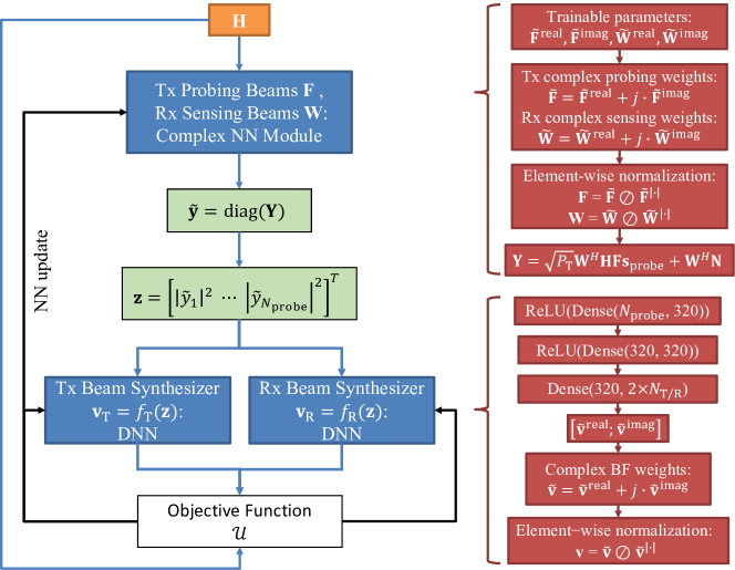
Figure 2: The architecture of the proposed NN, including the probing beam pairs $\mathbf{F}$ and $\mathbf{W}$ and the beam selection functions $f_{\textnormal{T}}(\cdot)$ and $f_{\textnormal{R}}(\cdot)$. The Tx and Rx beam synthesizers have the same architecture.

III-C Practicality of the Proposed Method

The NN model is trained offline prior to deployment. The training data can be obtained through ray-tracing simulations or from measurements. Due to the difficulty of obtaining CSI in real time, online training and adaptation of the NN remain an open research problem. On the other hand, the model proves to be fairly robust against imperfect training data, as we will show in Section V-D2. After the offline training phase, the probing beam pairs are extracted from the complex NN module and implemented in RF. The beam synthesizers $f_{\mathrm{T}},f_{\mathrm{R}}$ are implemented at the BS and the UE respectively. During deployment, the BS and the UE periodically sweep the probing beam pairs while the UE measures the received signal power. The probing measurements are then reported to the BS. The BS and the UE use the probing measurements as inputs to $f_{\mathrm{T}}$ and $f_{\mathrm{R}}$ to synthesize the Tx and Rx beams. Since the probing beams and the beam synthesizers are site-specific, $\mathbf{W}$ and $f_{\mathrm{R}}$ need to be transmitted to the UE. In a non-standalone system, this can be done through a lower-frequency side link. A new UE can then complete IA using the strongest probing beam pair. We have previously shown that the Tx probing beams can be used for IA in the MISO setting [1]. Therefore in a standalone system, the BS may sweep the Tx probing beams while a new UE receives using a quasi-omnidirectional beam. The UE can complete IA with the strongest Tx probing beam, download the Rx components $\mathbf{W}$ and $f_{\mathrm{R}}$, then perform the full joint Tx-Rx beam alignment.

III-D Baselines and Metrics

The proposed method optimizes the GF beam synthesizers and the probing beam pairs through DL, hence is referred to as the DL-GF method. It will be compared with five baselines: the DL-CB method, the exhaustive search, the genie with DFT codebooks, the DFT+EGC method, and MRT+MRC. The same probing measurement spreading gain of $\beta$ is adopted in DL-GF, DL-CB and the exhaustive search for a fair comparison.

• DL-CB. The DL-CB method replaces the Tx and Rx beam synthesizers with two classifiers that predict the optimal beam indices in the BS and UE codebooks. It is an extension of our previous work [27] to the MIMO scenario. To improve its accuracy, the DL-CB method can sweep the top few candidate beam pairs predicted by the classifiers. In our experiment, the best beam pair is selected after trying all combinations of the top-3 predicted Tx and Rx beams.

• Exhaustive search. The exhaustive search sweeps and measures all combinations of beam pairs in the BS and UE codebooks and selects the beam pair with the highest received signal power. Since the measurements are corrupted by noise, the beam pair selected by the exhaustive search may not be the one maximizing SNR.

• Genie DFT. A genie always selects the optimal beam pair in the BS and UE codebooks. It is the same as the exhaustive search when the measurement noise power is zero.

• DFT+EGC. Only the BS has a codebook in the DFT+EGC baseline. The BS exhaustively tries all beams in its codebook while the UE uses the corresponding EGC vector for each Tx beam. The best beam pair is selected assuming no measurement noise. It is expected to perform better than the genie DFT baseline due to the additional degree of freedom at the UE.

• MRT+MRC. Neither the BS nor the UE uses a codebook. The BS uses the optimal MRT beam while the UE uses the MRC beam. The BF gain can be computed through an eigendecomposition of $\mathbf{H}^{H}\mathbf{H}$. The MRT+MRC baseline is the theoretical upper bound under the unit-power constraint and cannot be achieved under the stricter unit-modulus constraint.

One important performance metric for beam alignment is the SNR achieved by the selected beams. We will compare the average SNR as well as the SNR distribution across different baselines. Secondly, new UE need to satisfy a minimum SNR requirement so that they can be discovered during the IA process and connect to the BS. This is generally not a concern for CB approaches that adopt uniform codebooks, but may be problematic when the probing beams are site-specific and have severe coverage holes. Therefore, we will also investigate the misdetection probability of UE, which is the probability that a UE achieves below-threshold SNR with the strongest probing beam pair, formally defined as

$$P\Bigl{(}\max\limits_{i\in{1,\cdots,N_{\textnormal{probe}}}}\frac{P_{\textnormal{T}}|\mathbf{w}_{i}^{H}\mathbf{H}\mathbf{f}_{i}|^{2}}{\sigma^{2}}<\textnormal{SNR}_{\textnormal{TH}}\Bigr{)}.$$ (17)

The SNR threshold is chosen to be -5 dB [30].

IV Dataset

Four scenarios from the public DeepMIMO dataset [31] are considered to capture a wide range of propagation environments, including indoor and outdoor environments, 28 GHz and 60 GHz carrier frequencies, as well as LOS and NLOS UE. The channel realizations are computed through ray-tracing with a state-of-the-art commercial-grade software [32], which is one of the most accurate ways of simulating mmWave channels once the environment topology is specified. The BS and UE adopt UPA with half-wavelength spacing. The simulation parameters are summarized in Table I for the four scenarios described below.

TABLE I: Simulation Parameters

BS Antenna	$8\times 8$ UPA
BS Codebook Size	$16\times 16=256$
UE Antenna	$4\times 4$ UPA
UE Codebook Size	$8\times 8=64$
Antenna Element	Isotropic
Carrier Frequency	Outdoor LOS (O1): 28 GHz Indoor (I3): 60 GHz Outdoor NLOS (O1 blockage): 28 GHz
Bandwidth ($B$)	100 MHz
Transmit Power ($P_{T}$)	O1: 20 dBm I3, BS 1: 10 dBm I3, BS 2: 20 dBm O1 blockage: 35 dBm
Noise Power $\sigma^{2}$	-81 dBm
Probing Measurement Spreading Gain $\beta$	16
UE Orientation Range	$z:Unif(-\pi,\pi)$ $y:Unif(-\frac{\pi}{2},\frac{\pi}{2})$ $x:Unif(-\frac{\pi}{2},\frac{\pi}{2})$

O1 Scenario. The O1 scenario captures an outdoor urban street environment with LOS UE. An illustration of the scenario is shown in Fig. 3(a). We select BS 3 and UE from row #800 to row #1200 from the original dataset. The BS is placed on the street side and a total of 72,581 UE are placed on a uniform grid on the street. The carrier frequency is 28 GHz.

I3 Scenarios. The I3 scenarios captures an indoor office environment with both LOS and NLOS UE. An illustration of the environment is shown in Fig. 3(c). There are two BS in this scenario: BS 1 is placed on the inside wall of the conference room and BS 2 is placed on the opposite wall. A grid of LOS UE is placed inside the conference room and a grid of NLOS UE is placed in the corridor outside. There are a total of 118,959 UE and the carrier frequency is 60 GHz. We consider two scenarios based on this environment, each with one of the two BS activated.

O1 Blockage Scenario. The O1 blockage scenario is artificially created based on the O1 scenario with a metal screen placed in front of the BS and two reflectors placed on both ends of the street, as illustrated in Fig. 3(b). The carrier frequency is 28 GHz and there are a total of 497,931 UE positions. While it may not be representative of practical mmWave deployments, the extreme topology allows us to gain some intuition on the beam patterns learned in this environment.

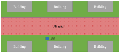
(a)

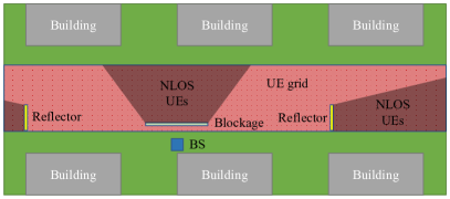
(b)

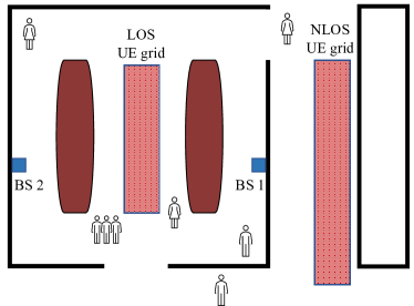
(c)

Figure 3: Illustration of the DeepMIMO ray-tracing scenarios.

V Evaluation

The datasets discussed in Section IV are partitioned so that 60% is used to train the NN, 20% is used for validation and hyper-parameter tuning, and the remaining 20% is used for testing. The NN are trained for 2000 epochs with a batch size of 800 using the ADAM optimizer [33]. The $\gamma$ parameter in the utility function is chosen to be 0.3 empirically to balance the SNR and IA performance. Operators may tune $\gamma$ individually for each deployment scenario as a hyperparameter. The measurement noise is AWGN. For CB baselines, the BS and the UE adopt over-sampled DFT codebooks with 256 and 64 beams respectively. The rest of the simulation parameters are summarized in Table I. The code for this work is published.

V-A Gain of DL-GF vs. Baselines

V-A1 Can DL-GF Achieve High SNR?

An ideal beam alignment method should quickly select near-optimal beams and achieve high SNR. The average SNR achieved by the proposed DL-GF method and the baselines in the more realistic O1 and I3 scenarios are shown in Fig. 4, 5, 6. It is evident that with the DL-CB approach, the beam classifiers can accurately select the best beam pairs. With an increasing number of probing beam pairs, the average SNR achieved by the DL-CB baseline approaches that by the genie DFT. Nevertheless, its performance is limited by the resolution of the BS and UE codebooks since there is still a 1 dB gap between the DFT+EGC baseline and the genie DFT. On the other hand, the proposed DL-GF method improves upon DL-CB with its fully synthesized beams and is able to beat the exhaustive search with 20 probing beam pairs in the O1 scenario, 12 in I3 with BS 1 activated, and 8 in I3 with BS 2 activated. It is eventually able to outperform the DFT+EGC baseline with as few as 20 probing beam pairs in the I3 scenarios and 32 in O1. A comparison of the 10th, 50th, 90th percentile and the average SNR with 32 probing beam pairs is shown in Table II. The proposed DL-GF method outperforms the exhaustive search everywhere in the distribution in both the O1 and the I3 scenario with BS 1 activated, and is only slightly worse in the 10th percentile SNR in the I3 scenario with BS 2 activated. Meanwhile, the misdetection probability is just 0.117$\%$, 0.013$\%$ and 2.422$\%$ in the O1, I3 BS 1 and I3 BS 2 environments, guaranteeing that the vast majority of UE can complete IA with one of the probing beams.

The gain of DL-GF is twofold. First, in the probing phase, the site-specific probing and sensing beams allow the BS and the UE to capture crucial channel information with fewer measurements. Second, in the beam prediction phase, the beam synthesizer functions can be intuitively viewed as infinitely large codebooks, whose resolution in practice is only limited by the floating-point precision of the NN and the range of probing measurements. By generating analog beams at increased spatial resolutions that are also adapted to the specific environment, DL-GF achieves additional gain over the standard DFT codebooks. The proposed method can also be viewed to perform implicit channel estimation and beam alignment jointly. The probing phase is analogous to CS, where a few learned site-specific beams are used to sense the channel. As a result, the proposed method can approach and even beat baselines such as DFT+EGC which require full CSI.

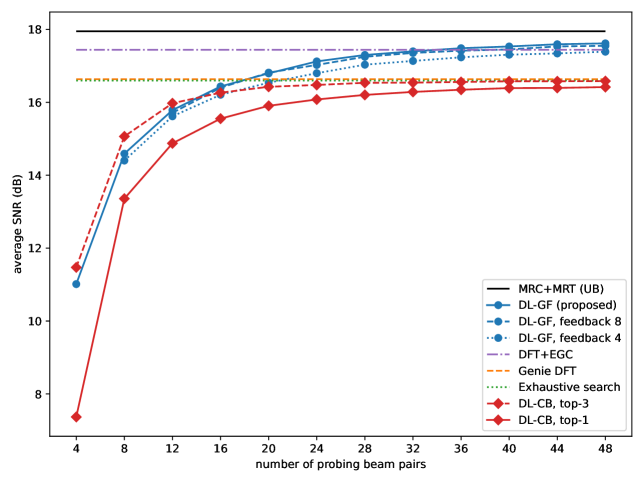
Figure 4: The average SNR vs. number of probing beam pairs in the O1 scenario.

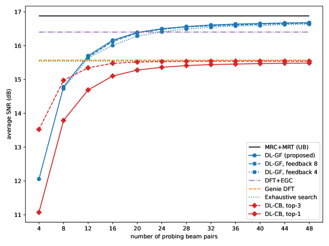
Figure 5: The average SNR vs. number of probing beam pairs in the I3 BS 1 scenario.

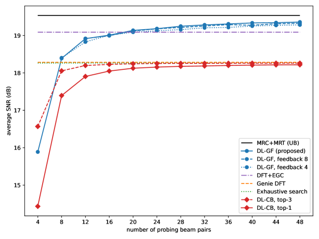
Figure 6: The average SNR vs. number of probing beam pairs in the I3 BS 2 scenario.

TABLE II: SNR Comparison with 32 Probing Beam Pairs

Scenario	SNR (dB)	DL-GF	DL-CB top-3	Exhaustive search	Genie DFT	DFT+EGC	MRT+MRC
O1 (misdetection probability = 0.117%)	10th %	11.249	10.591	10.630	10.835	11.744	12.421
	50th %	16.286	15.310	15.315	15.365	16.217	16.707
	90th %	20.513	19.661	19.713	19.723	20.517	20.918
	average	17.398	16.540	16.597	16.634	17.440	17.949
I3, BS 1 (misdetection probability = 0.013%)	10th %	13.804	12.535	12.535	12.624	13.805	14.316
	50th %	16.513	15.351	15.353	15.385	16.269	16.771
	90th %	18.349	17.472	17.472	17.480	18.170	18.518
	average	16.611	15.541	15.542	15.572	16.402	16.879
I3, BS 2 (misdetection probability = 2.422%)	10th %	5.327	5.492	5.793	6.185	7.246	8.090
	50th %	17.641	16.571	16.614	16.635	17.672	18.167
	90th %	23.385	22.348	22.351	22.358	23.131	23.529
	average	19.283	18.255	18.262	18.283	19.089	19.535

V-A2 The SNR vs. Beam Alignment Speed Trade-off

Conventional CB beam alignment approaches can always find better beams more frequently by trying more candidates and increasing the resolution of the codebook. Similarly, the proposed DL-GF method can achieve better SNR by sweeping more probing beams. However, such SNR gain usually occurs at the cost of higher latency. In practical cellular systems with multiple UE, the beam alignment procedure may need to be performed for each UE. It is therefore important for operators to consider the trade-off between the SNR and the overall beam alignment speed, which we define as the reciprocal of the total number of beams swept for all UE. The average SNR achieved at each beam alignment speed for DL-GF, DL-CB and the exhaustive search is shown in Fig. 7. Compared to the exhaustive search, the proposed DL-GF method is better by 5 to 10 dB in terms of the average SNR at a given speed or faster by around two orders of magnitude when the achieved average SNR is from 10 to 15 dB. The proposed GF approach is also strictly better than the CB method, achieving 1-2.5 dB higher SNR at each beam alignment speed. With multiple UE, other beam alignment methods that require an additional beam sweeping phase for each UE are expected to achieve a similar SNR-speed trade-off as the DL-CB with top-$k$ search does. Since DL-GF is faster than DL-CB with top-3 search by an order of magnitude with 10 or 20 UE, similar gains can be expected over methods such as the hierarchical search and active learning approaches. Interestingly, increasing the number of probing beams is often more efficient than searching more candidates for the DL-CB method, particularly when a high beam alignment speed is required.

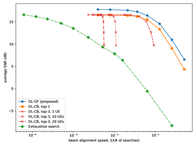
Figure 7: Average SNR vs. the total beam alignment speed in the O1 scenario.

A more detailed analysis of the total number of beams swept for different beam alignment methods in a cell with $K$ UE is shown in Table III. In the hierarchical search, the BS and the UE adopt 2-tier codebooks with $N_{\mathbf{F}}$ and $N_{\mathbf{W}}$ wide beams respectively. The BS first performs the Tx hierarchical search while the UE uses an omnidirectional Rx beam, then the UE performs the Rx hierarchical search. The exhaustive search requires sweeping all combinations of the $M_{\textnormal{T}}$ Tx beams and $M_{\textnormal{R}}$ Rx beams, which amounts to a total of 16,384 beam pairs in our setting. Methods such as the hierarchical search and DL-CB with top-$k$ search require an additional beam sweeping phase for each UE. As a result, the overall beam sweeping overhead increases linearly with the number of UE. On the other hand, since the proposed DL-GF method predicts the beams in one shot after sweeping a common set of probing beam pairs for all UE, its beam sweeping overhead is constant regardless of the number of UE. In our setting, DL-GF reduces the beam sweeping overhead by over 500$\times$ while scaling optimally with increasing number of UE.

TABLE III: Beam Sweeping Overhead for $K$ UEs

Beam alignment method	Beam sweeping overhead	Feedback overhead
DL-GF	$N_{\textnormal{probe}}$	$KN_{\textnormal{probe}}$ power values
DL-CB, top-$k$	$N_{\textnormal{probe}}+\min(K\cdot k_{\mathbbm{1}_{\{k>1\}}},M_{\textnormal{T}}M_{\textnormal{R}})$	$KN_{\textnormal{probe}}$ power values + $K\cdot\mathbbm{1}_{\{k>1\}}$ beam indices
Hierarchical search with $N_{\mathbf{F}},N_{\mathbf{W}}$ Tx and Rx wide beams	$N_{\mathbf{F}}+\min(K\frac{M_{\textnormal{T}}}{N_{\mathbf{F}}},M_{\textnormal{T}})+N_{\mathbf{W}}+\min(K\frac{M_{\textnormal{R}}}{N_{\mathbf{W}}},M_{\textnormal{R}})$	$4K$ beam indices
Exhaustive search of $M_{\textnormal{T}},M_{\textnormal{R}}$ Tx and Rx beams	$M_{\textnormal{T}}M_{\textnormal{R}}$	$K$ beam indices

V-B Intuition Behind the Learned Beams

To better understand how the probing beam pairs and the beam synthesizer functions achieve better performance, we investigate the learned beam patterns in the O1 Blockage scenario without random UE orientations. For easier visualization, the BS and the UE are equipped with ULA arrays that only beamform in the azimuth domain. A UE located on the left of the BS is selected from the testing dataset as a case study. With 4 probing beam pairs, the probing and sensing beam patterns are heavily adapted to the propagation environment by directing most of the energy towards the reflectors on both ends of the street while avoiding the blockage in the broadside direction, as shown in Fig. 8. The probing and sensing beams often have multiple lobes, which likely allows them to capture channel information more effectively. On the other hand, the synthesizers predict sub-optimal beams. Both the Tx and Rx beams have a single narrow main lobe, but are misaligned with the dominant path by 2.51 and 1.79 degrees respectively. As the number of probing beam pairs is increased to 24, the learned probing beams have much larger spatial coverage, as shown in Fig. 9. This is particularly noticeable in the Rx sensing beams since the range of AoA is much larger compared to that of the AoD with more variations in the location of UE. Utilizing the increased information gathered by the probing beam pairs, the beam synthesizers also learn to focus energy more accurately. Both the predicted Tx and Rx beams are better aligned with the dominant path and are off by just 0.73 degrees. Overall, this allows DL-GF to achieve better SNR by adopting more probing beams.

\begin{overpic}[width=433.62pt]{Figures/O1_28B_BS_3_64x16_MIMO_ULA_4_probing_beams_probing_beam_pattern.pdf} \put(0.0,160.0){\small\noindent\hbox{}\hfill{{\hbox{\begin{tabular}[c]{@{}c@{}}highly site-specific\\ probing spatial coverage\\ to avoid blockage\end{tabular}}}}\hfill\hbox{}} \end{overpic}

(a) Learned probing beam pairs

\begin{overpic}[width=433.62pt]{Figures/O1_28B_BS_3_64x16_MIMO_ULA_4_probing_beams_predicted_beam_pattern.pdf} \put(0.0,160.0){\small\noindent\hbox{}\hfill{{\hbox{\begin{tabular}[c]{@{}c@{}}narrow predicted beams\\ slightly misaligned with\\ the dominant path\end{tabular}}}}\hfill\hbox{}} \end{overpic}

(b) Predicted beam pair for communication

Figure 8: Radiation patterns of learned probing beam pairs and predicted beams in the O1 blockage scenario, $N_{\mathrm{probe}}=4$.

\begin{overpic}[width=433.62pt]{Figures/O1_28B_BS_3_64x16_MIMO_ULA_24_probing_beams_probing_beam_pattern.pdf} \put(20.0,160.0){\small\noindent\hbox{}\hfill{{\hbox{\begin{tabular}[c]{@{}c@{}}increased probing\\ spatial coverage\end{tabular}}}}\hfill\hbox{}} \end{overpic}

(a) Learned probing beam pairs

\begin{overpic}[width=433.62pt]{Figures/O1_28B_BS_3_64x16_MIMO_ULA_24_probing_beams_predicted_beam_pattern.pdf} \put(0.0,160.0){\small\noindent\hbox{}\hfill{{\hbox{\begin{tabular}[c]{@{}c@{}}narrow predicted beams\\ closely aligned with\\ the dominant path\end{tabular}}}}\hfill\hbox{}} \end{overpic}

(b) Predicted beam pair for communication

Figure 9: Radiation patterns of learned probing beam pairs and predicted beams in the O1 blockage scenario, $N_{\mathrm{probe}}=24$.

V-C Validating the Proposed Design

V-C1 Benefits of Site-specific Probing

The learned probing beam pairs provide important information about the channel for the downstream NN beam synthesizers. To verify the benefits of site-specific probing, the learned probing and sensing beams are replaced with evenly spaced pencil beams from sub-sampled DFT codebooks. Compared to learning site-specific probing beam pairs, the average SNR drops by over 10 dB when both the BS and the UE adopt DFT beams as shown in Fig. 10. Note that in this setting, the UE measures and reports all combinations of the probing and sensing beams so that the total number of probing beam pairs is $N_{\textnormal{probe}}^{2}$. If the BS learns site-specific probing beams while the UE adopts DFT sensing beams, there is still a 2 dB loss in the average SNR. Therefore, learning site-specific probing and sensing beams for the BS and the UE can provide significant gain.

The proposed method learns a UE beam for each BS probing beam. An alternative strategy is to measure all combinations of probing and sensing beams and feed back all the measurements, which requires a total number of $N_{\textnormal{probe}}^{2}$ probing beam pairs instead of $N_{\textnormal{probe}}$ in the proposed design. As shown in Fig. 10, this approach is consistently worse than the proposed design, particularly when the number of probing beam pairs is small. Feeding back only the maximum Rx measurement for each BS probing beam results in little further performance degradation when using more than 25 probing beam pairs. This indicates that most of the sensing measurements for each probing beam provide little additional information about the channel. Overall, the proposed probing strategy can capture information about the channel more efficiently with a limited number of probing measurements.

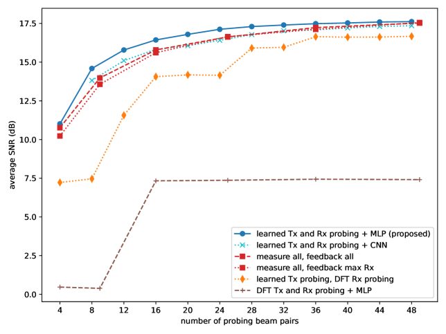
Figure 10: Average SNR vs. the number of probing beam pairs with different probing beam designs, probing strategies and NN architectures in the O1 scenario.

V-C2 Verifying the Beam Synthesizer Architecture

The NN beam synthesizers use a fully connected MLP architecture due to the relatively small feature dimension. For comparison, an alternative beam synthesizer is designed with 3 one-dimensional convolutional layers followed by max pooling with a stride of 2 and a kernel size of 2, flattening, and a final fully connected output layer. Each convolutional layer has 64 channels, a kernel size of 3 and ReLU activation. As shown in Fig. 10, the proposed design consistently achieves better average SNR than the CNN-based design does, indicating that the MLP is an appropriate architecture in this setting.

V-C3 Reducing the Misdetection Probability

The ideal beam alignment solution should not only achieve high BF gain for connected UE, but also be able to discover new UE and allow them to complete IA. With the proposed DL-GF method, a new UE can do so with one of the probing beam pairs if it satisfies a minimum SNR requirement. Naturally, adopting more probing beams will allow each to cover a smaller angular space, thus increasing the gain of the probing beams and reducing the misdetection probability. By explicitly incorporating the IA performance in the utility function, we provide another tuning nob to reduce the misdetection probability. The proposed utility function can indeed further reduce the misdetection probability when the number of probing beam pairs is fixed, as shown in Fig. 11. Compared to simply optimizing the BF gain of the synthesized beams ($\gamma=1.0$), incorporating the IA performance ($\gamma=0.3$) reduces the misdetection probability by 6.3 percentage points with 8 probing beam pairs and by 3.2 percentage points with 12 probing beam pairs while suffering from little SNR loss. Although the gain diminishes with more probing beams, the two-component utility function still provides a powerful tool to improve the IA coverage when the number of probing beams is limited. Since the $\mathcal{U}_{\textnormal{IA}}$ term only covers UE below a specified SNR threshold, the proposed utility function also allows the NN model to adapt to different SNR requirements for IA. As shown in Fig. 12, the misdetection probability is reduced at various SNR threshold values for IA compared to simply optimizing the BF gain. The gain is more significant if a higher SNR threshold is required.

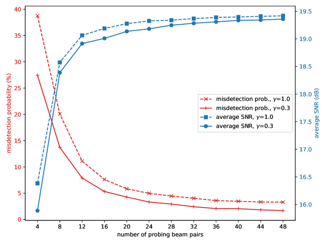
Figure 11: The misdetection probability and average SNR vs. the number of probing beam pairs with different $\gamma$ during training in the I3 scenario with BS 2 activated.

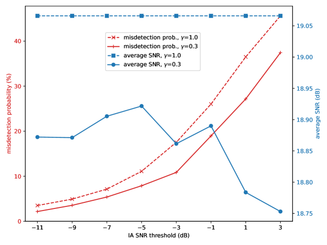
Figure 12: The misdetection probability and average SNR vs. the IA SNR threshold with different $\gamma$ in the I3 scenario with BS 2 activated. The proposed method uses 12 probing beam pairs.

V-D Robustness of DL-GF

V-D1 Robustness to Noisy Measurements

The beam synthesizers rely on the probing measurements to generate the BF weights. While measurement noise can cause search errors in exhaustive and hierarchical searches, it can also impact the prediction of the NN models. A comparison of the average SNR achieved by the predicted beams with increasing probing measurement spreading gain is shown in Fig. 13. Both DL-based methods are trained at each probing measurement spreading gain level. As expected, the performance of the DL-GF, DL-CB and exhaustive search improves with increasing measurement spreading gain. The exhaustive search benefits less: its performance plateaus with almost no measurement spreading gain. On the other hand, the proposed DL-GF and the DL-CB methods are less robust to measurement noise due to their probing beams having lower gain. They both require a spreading gain of around 12 dB in the probing measurements to achieve their best performance. To further investigate the impact of noise, negative spreading gain is considered, which implies a setting where the measurements are noisier during probing than in data transmission. Interestingly, the average SNR of the exhaustive search drops sharply and becomes the worst when the measurements are extremely noisy. At this point, the exhaustive search essentially produces random guesses since the beam measurements are dominated by noise. On the other hand, the DL-based methods converge to always predict the same beam pair. In the case of DL-CB, the predicted beam pair happens to be the most frequent optimal beam pair.

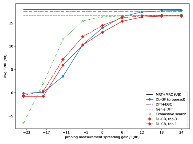
Figure 13: Comparison of the average SNR with increasing spreading gain in the probing measurements in the O1 scenario. The DL-GF and DL-CB methods have 32 probing beam pairs. A negative spreading gain means measurements during probing are noisier than in data transmission.

V-D2 Robustness to Imperfect Training Data

Training DL models typically requires high-quality data. While ray-tracing is one of the most accurate ways to simulate mmWave channels, it is not easily scalable to a city-wide deployment and the generated data may still differ from actual channels due to mismatched environments and imperfect propagation models. If the training data is acquired through measurement campaigns, noisy measurement and channel estimation errors would also affect the quality of the data. It is therefore important to investigate the performance of the proposed method when there is a mismatch between the channels used for training and the actual channels during deployment. To simulate imperfect training data, the training channel matrices are corrupted with AWGN while the model is tested on clean channel data. The average SNR of the proposed DL-GF method, the DL-CB baseline and the exhaustive search with increasing NMSE in the training data is shown in Fig. 14. Both the DL-GF and the DL-CB methods are relatively robust to noisy training data, experiencing little performance degradation when the channel NMSE is smaller than -3 dB. A small amount of noisy in the training data actually benefits the proposed DL-GF method, which is a common phenomenon in ML where noisy training data can sometimes improve the robustness and generalizability of ML models [34]. Even with a channel NMSE of 1 dB, the proposed DL-GF method can still outperform the exhaustive search and the DL-CB baseline trained on clean data. The added noise likely does not fundamentally shift the distribution of channels but instead makes it more “fuzzy”. During the unsupervised training procedure, the proposed NN still learn to beamform on these noisy channels and generalize well to the clean actual channels.

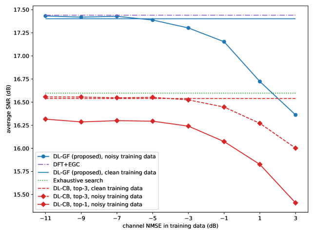
Figure 14: Comparison of the average SNR with increasing training channel NMSE in the O1 scenario. The DL-GF and DL-CB methods have 32 probing beam pairs.

V-D3 Reducing the Feedback Overhead

The gain of DL-GF can be partially attributed to the much richer uplink feedback: it uses all the measurements as feature vectors to synthesize the BF weights instead of simply selecting the strongest beam. The feedback overhead of different methods are summarized in Table III. To reduce the feedback overhead, UE can report measurements of a few strongest probing beam pairs so that UE use all the measurements to synthesize their beams while the BS uses only the reported measurements. The Rx beam synthesizer $f_{\textnormal{R}}$ takes the full measurement vector $\mathbf{z}$ as input. The Tx beam synthesizer $f_{\textnormal{T}}$ takes a masked version of $\mathbf{z}$ so that only the top-$m$ highest measurements are non-zero. Since the shape of the feature vector is roughly maintained, reducing the feedback only results in a small degradation in the average SNR, as shown in Fig. 4, 5, 6. For instance, in the O1 scenario with 32 probing beam pairs in total, the average SNR drops by 0.263 dB when reporting 4 beam pairs and by only 0.043 dB when reporting the best 8.

V-D4 Impact of Random UE Orientations

The orientation of UE has a large impact on the performance of the proposed DL-GF method. A comparison of the average SNR and the misdetection probability with and without random UE rotation in the O1 scenario is shown in Fig. 15. Without random UE rotation, the proposed method can achieve better average SNR and lower misdetection probability with significantly fewer probing beam pairs. The random UE rotation increases the effective range of AoA. As a result, more probing beam pairs are required to capture sufficient channel information on the UE side. The UE’s sensing beams also need to distribute energy and cover a larger angular space, leading to reduced BF gain and worse misdetection probability.

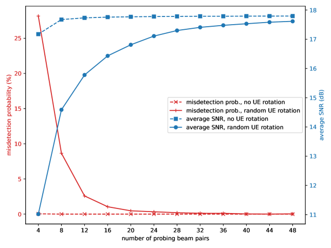
Figure 15: The average SNR and misdetection probability of the proposed DL-GF method with and without random UE orientations in the O1 scenario.

VI Conclusion

The proposed GF approach provides a promising new paradigm for mmWave beam alignment by achieving better SNR while being faster than existing methods by orders of magnitude. Its gain can be attributed to the combination of site-specific adaptation and the joint optimization of channel probing and beam synthesis. Next-generation cellular systems can reap the benefits without overhauling the existing beam sweeping-based framework: the probing beams can be transmitted using periodic RS while traditional beamforming codebooks are replaced with NN beam synthesizers. Operators can select the number of probing beam pairs based on the SNR and IA coverage requirement for each site.

There are many possible directions that this line of research could be extended, many of which have been identified throughout the paper. For example, scaling the site-specific training to city-wide networks and online adaptation to dynamic environments remain open research problems. Multi-beam and multi-UE communication including the joint optimization of analog and digital BF is another promising direction. The beam alignment problem has mostly been investigated to date from the BS point of view. It is important to also consider the unique beam alignment challenges on the UE side arising from multiple antenna panels, precarious dynamic rotations and more demanding power management.

References

- [1] Y. Heng and J. G. Andrews, “Grid-less mmWave beam alignment through deep learning,” in Proc. IEEE GLOBECOM. IEEE, Dec. 2022, pp. 2290–2295.
- [2] M. Giordani, M. Polese, A. Roy, D. Castor, and M. Zorzi, “A tutorial on beam management for 3GPP NR at mmWave frequencies,” IEEE Commun. Surv. Tut., vol. 21, no. 1, pp. 173–196, Sep. 2019.
- [3] Y. Heng, J. G. Andrews, J. Mo, V. Va, A. Ali, B. L. Ng, and J. C. Zhang, “Six key challenges for beam management in 5.5G and 6G systems,” IEEE Commun. Mag., vol. 59, no. 7, pp. 74–79, Jul. 2021.
- [4] Z. Xiao, T. He, P. Xia, and X.-G. Xia, “Hierarchical codebook design for beamforming training in millimeter-wave communication,” IEEE Trans. Wireless Commun., vol. 15, no. 5, pp. 3380–3392, May 2016.
- [5] C. Qi, K. Chen, O. A. Dobre, and G. Y. Li, “Hierarchical codebook-based multiuser beam training for millimeter wave massive MIMO,” IEEE Trans. Wireless Commun., vol. 19, no. 12, pp. 8142–8152, Sep. 2020.
- [6] A. Ali, N. González-Prelcic, and R. W. Heath, “Millimeter wave beam-selection using out-of-band spatial information,” IEEE Trans. Wireless Commun., vol. 17, no. 2, pp. 1038–1052, Feb. 2018.
- [7] Y. Heng and J. G. Andrews, “Machine learning-assisted beam alignment for mmWave systems,” IEEE Trans. Cogn. Commun. Netw., vol. 7, no. 4, pp. 1142–1155, May 2021.
- [8] V. Va, J. Choi, T. Shimizu, G. Bansal, and R. W. Heath, “Inverse multipath fingerprinting for millimeter wave V2I beam alignment,” IEEE Trans. Veh. Technol., vol. 67, no. 5, pp. 4042–4058, Dec. 2017.
- [9] N. González-Prelcic, R. Méndez-Rial, and R. W. Heath, “Radar aided beam alignment in mmWave V2I communications supporting antenna diversity,” in Proc. Inf. Theory and Appl. Workshop (ITA), Feb. 2016, pp. 1–5.
- [10] U. Demirhan and A. Alkhateeb, “Radar aided 6G beam prediction: Deep learning algorithms and real-world demonstration,” in Proc. IEEE WCNC, Apr. 2022, pp. 2655–2660.
- [11] B. Salehihikouei, G. Reus-Muns, D. Roy, Z. Wang, T. Jian, J. Dy, S. Ioannidis, and K. Chowdhury, “Deep learning on multimodal sensor data at the wireless edge for vehicular network,” IEEE Trans. Veh. Technol., vol. 71, no. 7, pp. 7639–7655, Apr. 2022.
- [12] W. Xu, F. Gao, S. Jin, and A. Alkhateeb, “3D scene-based beam selection for mmWave communications,” IEEE Wireless Commun. Letters, vol. 9, no. 11, pp. 1850–1854, Jun. 2020.
- [13] S. H. Lim, S. Kim, B. Shim, and J. W. Choi, “Deep Learning-Based Beam Tracking for Millimeter-Wave Communications Under Mobility,” IEEE Trans. Commun., vol. 69, no. 11, pp. 7458–7469, Aug. 2021.
- [14] F. B. Mismar, B. L. Evans, and A. Alkhateeb, “Deep reinforcement learning for 5G networks: Joint beamforming, power control, and interference coordination,” IEEE Trans. Commun., vol. 68, no. 3, pp. 1581–1592, Mar. 2020.
- [15] Q. Xue, Y.-J. Liu, Y. Sun, J. Wang, L. Yan, G. Feng, and S. Ma, “Beam management in ultra-dense mmWave network via federated reinforcement learning: An intelligent and secure approach,” IEEE Trans. Cogn. Commun. Netw., Oct. 2022.
- [16] K. Ma, Z. Wang, W. Tian, S. Chen, and L. Hanzo, “Deep learning for mmWave beam-management: State-of-the-art, opportunities and challenges,” IEEE Wireless Commun., pp. 1–8, Aug. 2022.
- [17] M. Qurratulain Khan, A. Gaber, P. Schulz, and G. Fettweis, “Machine learning for millimeter wave and terahertz beam management: A survey and open challenges,” IEEE Access, vol. 11, pp. 11 880–11 902, Feb. 2023.
- [18] M. N. Khormuji and R.-A. Pitaval, “Statistical beam codebook design for mmWave massive MIMO systems,” in Proc. IEEE EuCNC, Jun. 2017, pp. 1–5.
- [19] W. Liu and Z. Wang, “Statistics-assisted beam training for mmWave massive MIMO systems,” IEEE Commun. Letters, vol. 23, no. 8, pp. 1401–1404, Jun. 2019.
- [20] M. Alrabeiah, Y. Zhang, and A. Alkhateeb, “Neural networks based beam codebooks: Learning mmWave massive MIMO beams that adapt to deployment and hardware,” IEEE Trans. Commun., vol. 70, no. 6, pp. 3818–3833, Apr. 2022.
- [21] Y. Zhang, M. Alrabeiah, and A. Alkhateeb, “Reinforcement learning of beam codebooks in millimeter wave and terahertz MIMO systems,” IEEE Trans. Commun., vol. 70, no. 2, pp. 904–919, Nov. 2021.
- [22] W. Ma, C. Qi, and G. Y. Li, “Machine learning for beam alignment in millimeter wave massive MIMO,” IEEE Wireless Commun. Letters, vol. 9, no. 6, pp. 875–878, Jun. 2020.
- [23] X. Li and A. Alkhateeb, “Deep learning for direct hybrid precoding in millimeter wave massive MIMO systems,” in Proc. IEEE Asilomar, Nov. 2019, pp. 800–805.
- [24] D. J. Love and R. W. Heath, “Equal gain transmission in multiple-input multiple-output wireless systems,” IEEE Trans. Commun., vol. 51, no. 7, pp. 1102–1110, Jul. 2003.
- [25] K. M. Attiah, F. Sohrabi, and W. Yu, “Deep learning for channel sensing and hybrid precoding in TDD massive MIMO OFDM systems,” IEEE Trans. Wireless Commun., Jul. 2022, early access.
- [26] F. Sohrabi, T. Jiang, W. Cui, and W. Yu, “Active sensing for communications by learning,” IEEE Journal on Sel. Areas in Communications, vol. 40, no. 6, pp. 1780–1794, Mar. 2022.
- [27] Y. Heng, J. Mo, and J. G. Andrews, “Learning site-specific probing beams for fast mmWave beam alignment,” IEEE Trans. Wireless Commun., vol. 21, no. 8, pp. 5785–5800, Jan. 2022.
- [28] 3GPP, “Technical Specification Group Radio Access Network; Study on channel model for frequencies from 0.5 to 100 GHz,” 3rd Generation Partnership Project (3GPP), Technical Report (TR) 38.901, Dec. 2019, version 16.1.0.
- [29] C. N. Barati, S. A. Hosseini, S. Rangan, P. Liu, T. Korakis, S. S. Panwar, and T. S. Rappaport, “Directional cell discovery in millimeter wave cellular networks,” IEEE Trans. Wireless Commun., vol. 14, no. 12, pp. 6664–6678, Jul. 2015.
- [30] M. Giordani, M. Mezzavilla, and M. Zorzi, “Initial access in 5G mmWave cellular networks,” IEEE Commun. Mag., vol. 54, pp. 40–47, Nov. 2016.
- [31] A. Alkhateeb, “DeepMIMO: A generic deep learning dataset for millimeter wave and massive MIMO applications,” in Proc. Inf. Theory and Appl. Workshop (ITA), Feb. 2019, pp. 1–8.
- [32] Wireless InSite 3.2.0 Reference Manual, Remcom Inc., 2017. [Online]. Available: https://www.remcom.com/wireless-insite-em-propagation-software/
- [33] D. P. Kingma and J. Ba, “Adam: A method for stochastic optimization,” in Proc. ICLR, 2015.
- [34] I. Goodfellow, Y. Bengio, and A. Courville, Deep Learning. MIT Press, 2016, ch. 7, [Online.] Available: http://www.deeplearningbook.org.