Thompson Sampling with Virtual Helping Agents

Kartik Anand Pant    Amod Hegde    and K. V. Srinivas    \IEEEmembershipMember, IEEE This paragraph of the first footnote will contain the date on which you submitted your paper for review. It will also contain support information, including sponsor and financial support acknowledgment.Kartik Anand Pant is with Purdue University, USA. This work was done while he was student at the Electronics Engineering Department, IIT (BHU), Varanasi, India (e-mail: kpant@purdue.edu).Amod Hegde is with Stanford University, USA. This work was done while he was student at the Electronics Engineering Department, IIT (BHU), Varanasi, India (e-mail: amod96@stanford.edu).K. V. Srinivas is with Motorola Mobility, Canada. This work was done while he was working at the Electronics Engineering Department, IIT (BHU), Varanasi, India (e-mail: kvsrinivas@ieee.org).This paragraph will include the Associate Editor who handled your paper.
Abstract

We address the problem of online sequential decision making, i.e., balancing the trade-off between exploiting the current knowledge to maximize immediate performance and exploring the new information to gain long-term benefits using the multi-armed bandit framework. Thompson sampling is one of the heuristics for choosing actions that address this exploration-exploitation dilemma. We first propose a general framework that helps heuristically tune the exploration versus exploitation trade-off in Thompson sampling using multiple samples from the posterior distribution. Utilizing this framework, we propose two algorithms for the multi-armed bandit problem and provide theoretical bounds on the cumulative regret. Next, we demonstrate the empirical improvement in the cumulative regret performance of the proposed algorithm over Thompson Sampling. We also show the effectiveness of the proposed algorithm on real-world datasets. Contrary to the existing methods, our framework provides a mechanism to vary the amount of exploration/ exploitation based on the task at hand. Towards this end, we extend our framework for two additional problems, i.e., best arm identification and time-sensitive learning in bandits and compare our algorithm with existing methods.

{IEEEImpStatement}

The Multi-Armed Bandit problem has been extensively studied in the last decade. It has wide-ranging applications from clinical trials to product assortment. Recently, it has been utilized in web advertisements and recommendation systems. Thompson sampling (TS) provides a simple heuristic solution to the MAB problem with sub-linear regret bounds. However, TS doesn’t provide control over the amount of exploration and exploitation executed by the policy. In this letter, we provide an extension to TS allowing variation in the exploration and exploitation in TS with strong theoretical guarantees. We believe that our framework can be easily augmented with the existing TS based solution and enhance its performance. Our work finds its application even in scenarios where the objective is to find satisficing (nearly optimal) actions on a short horizon or best actions over a long time horizon.

{IEEEkeywords}

Multi-arm Bandits, Thompson sampling, Sequential Decision Making, Gaussian Bandits.

1 Introduction

\IEEEPARstart

In a stochastic multi-armed bandit (MAB) setting, an agent faces the problem of sequential decision making in the face of uncertainty. At each time step, the agent takes an action from a set of actions and each action produces a reward drawn from an underlying, fixed but unknown, distribution associated with that action. As the agent observes the reward at each time step, she learns about the underlying reward distributions and tries to optimize her long-term performance. The agent faces the dilemma of exploiting the already acquired knowledge to maximize her immediate rewards or exploring actions from which few/no observations have been made to acquire more knowledge for potential future gains while facing the risk of immediate loss.

Various algorithms have been proposed to solve the exploitation-exploration dilemma in the stochastic MAB problem. They include simple heuristics such as greedy and ϵitalic-ϵ\epsilon-greedy algorithms [1], computationally intensive approaches such as Gittins indices [2], and the Upper Confidence Bound (UCB) family of algorithms which offer low computational cost and strong theoretical guarantees on the performance [3], [4], [5], [6], [7], [8].

Thompson proposed a simple heuristic for the stochastic MAB with Bernoulli rewards [9]. Starting with a prior distribution over the unknown parameters of the reward distribution of each action, the algorithm updates the posterior distributions as the actions are played. At each time step, an action is chosen according to its posterior probability of being the best action. This algorithm is known as Thompson sampling (TS) (and also as posterior sampling, probability matching) and has attracted a lot of attention in recent times. While [10], [11], [12], [13], [14] presented empirical studies showing excellent performance of TS in comparison with other state-of-the-art algorithms along with some weak theoretical guarantees of TS, [15], [16], [17], [18], [19] and [20] have presented rigorous theoretical analysis establishing tight bounds on the regret performance of TS.

In this paper, we present a modified TS algorithm, referred to as Thompson Sampling with Virtual Helping Agents and Combining (TS-VHA-𝖢𝖢\mathsf{C}). The real (or, primary) agent playing the MAB game is assisted by N1>0𝑁10N-1>0 virtual helping agents, with each agent generating an independent sample from the posterior distribution of each arm; All the N𝑁N samples (N1𝑁1N-1 samples generated by the N1𝑁1N-1 virtual helping agents and the one generated by the primary agent), corresponding to each arm, are processed using a combiner and which arm to play next is decided based on the values of the combined samples. Here, we propose two linear combiners 𝖢𝟣𝖢𝟣\mathsf{C1} and 𝖢𝟤𝖢𝟤\mathsf{C2}. Compared to the (conventional) TS, 𝖢𝟣𝖢𝟣\mathsf{C1} increases the exploitation at the expense of exploration and 𝖢𝟤𝖢𝟤\mathsf{C2} increases the exploration at the expense of exploitation.

Importantly, our work may be considered as a framework for varying exploration vs. exploitation for Thompson sampling, by choosing the number of virtual helping agents and the type of combiner, enabling us to achieve a better regret performance (compared to TS) for some of the MAB problems. It is to be noted that one can design other combiners that achieve a different exploitation-exploration tradeoff.

Rest of the paper is organized as follows. After introducing the details of stochastic MAB problem and the Thompson sampling in Section 2, we present the TS-VHA algorithm in Section 3. Section 4 states the main theoretical results that we present and the corresponding proofs. In Section 5, we present simulation results to substantiate our theoretical results and Section 6 concludes the paper.

2 The Stochastic Multi-armed Bandit Problem

Consider an agent faced with a stochastic MAB problem. Given a slot machine with K𝐾K arms, the agent has to choose an arm to play at each time step t>0𝑡subscriptabsent0t\in\mathbb{Z}_{>0}. The real-valued reward produced by each arm, when played, is a random variable whose distribution is fixed but unknown with a finite support over [0,1]01[0,1]. The rewards obtained by playing an arm repeatedly are independent and identically distributed (i.i.d) and are independent of the plays of the other arms. The agent has to decide which arm to play at each time t𝑡t, based on its observations of the past t1𝑡1t-1 plays and their outcomes, to maximize the expected total reward at time T𝑇T, a widely used performance metric in the stochastic MAB setting. The set of arms can also be referred to as the set of actions and playing arm i𝑖i is equivalent to choosing action i𝑖i.

Denoting the (unknown) expected reward of arm i𝑖i with μisubscript𝜇𝑖\mu_{i} and the index of the arm played at time t𝑡t with i(t)𝑖𝑡i(t), the expected total reward at time T𝑇T is given by 𝔼[t=1Tμi(t)]𝔼delimited-[]superscriptsubscript𝑡1𝑇subscript𝜇𝑖𝑡\mathbb{E}\left[\sum_{t=1}^{T}\mu_{i(t)}\right]. An equivalent (and convenient) metric to work with is the expected total regret, given by

𝔼[R(T)]=𝔼[t=1Tμμi(t)],𝔼delimited-[]𝑅𝑇𝔼delimited-[]superscriptsubscript𝑡1𝑇superscript𝜇subscript𝜇𝑖𝑡\mathbb{E}[R(T)]=\mathbb{E}\left[\sum_{t=1}^{T}\mu^{*}-\mu_{i(t)}\right], (1)

where μmaxiμisuperscript𝜇subscript𝑖subscript𝜇𝑖\mu^{\ast}\coloneqq\max_{i}\mu_{i} and the expectation is over the random choices of arms played by the algorithm.

2.1 Thompson Sampling

As stated before, Thompson sampling takes a Bayesian approach. It starts by assuming an independent prior belief P(μ~i)𝑃subscript~𝜇𝑖P(\tilde{\mu}_{i}) over the expected reward of each arm i𝑖i and a likelihood function P(rμ~i)𝑃conditional𝑟subscript~𝜇𝑖P(r\mid\tilde{\mu}_{i}) representing the probability of observing reward r𝑟r upon playing arm i𝑖i. When an arm i𝑖i is played, its posterior is updated based on the observed reward r𝑟r using the Bayes rule: P(μ~ir)P(rμ~i)P(μ~i)proportional-to𝑃conditionalsubscript~𝜇𝑖𝑟𝑃conditional𝑟subscript~𝜇𝑖𝑃subscript~𝜇𝑖P(\tilde{\mu}_{i}\mid r)\propto P(r\mid\tilde{\mu}_{i})P(\tilde{\mu}_{i}). At each time t𝑡t, an arm is played according to its posterior probability of having the highest mean reward; In practice, this is done by simply drawing a sample from the posterior distribution of each arm and playing the arm that produces the largest sample. Algorithm 1 presents the Thompson sampling.

Algorithm 1 Thompson Sampling (TS)
0:  K𝐾K, priors P(μ^i)𝑃subscript^𝜇𝑖P(\hat{\mu}_{i}), likelihood P(rμ^i),i=1,,Kformulae-sequence𝑃conditional𝑟subscript^𝜇𝑖𝑖1𝐾P(r\mid\hat{\mu}_{i}),~{}i=1,\ldots,K.
  for each t=1,2,𝑡12t=1,2,\ldots do
     Sample:
     Draw θi(t)P(μ^i),i=1,,Kformulae-sequencesimilar-tosubscript𝜃𝑖𝑡𝑃subscript^𝜇𝑖𝑖1𝐾\theta_{i}(t)\sim P(\hat{\mu}_{i}),i=1,\ldots,K
     Select action:
     Play arm i(t)=argmaxiθi(t)𝑖𝑡subscript𝑖subscript𝜃𝑖𝑡i(t)=\arg\max_{i}\theta_{i}(t) and observe its reward r(t)𝑟𝑡r(t)
     Update distribution:
     P(μ^i(t))P(μ^i(t)r(t))𝑃subscript^𝜇𝑖𝑡𝑃conditionalsubscript^𝜇𝑖𝑡𝑟𝑡P(\hat{\mu}_{i(t)})\leftarrow P(\hat{\mu}_{i(t)}\mid r(t)), where P(μ^i(t)r(t))P(r(t)μ^i(t))P(μ^i(t))proportional-to𝑃conditionalsubscript^𝜇𝑖𝑡𝑟𝑡𝑃conditional𝑟𝑡subscript^𝜇𝑖𝑡𝑃subscript^𝜇𝑖𝑡P(\hat{\mu}_{i(t)}\mid r(t))\propto P(r(t)\mid\hat{\mu}_{i(t)})P(\hat{\mu}_{i(t)})
  end for

3 Thompson Sampling with Virtual Helping Agents

Thompson sampling has three essential steps. First, the agent draws a sample from the posterior distribution of the expected reward of each arm, which acts as an estimate of the arm’s expected reward. Next, the agent selects the arm with the largest sample and observes a reward. Finally, the agent updates the posterior distribution of the expected reward of the selected arm based on the observed reward.

Our proposed algorithm introduces two significant changes to the Thompson sampling. First, we modify the sampling step of TS by employing N1𝑁1N-1 virtual helping agents. Let 𝒦={1,2,,K}𝒦12𝐾\mathcal{K}=\{1,2,\ldots,K\} represent the set of arms and let 𝒜={1}{2,,N}={1,2,,N}𝒜12𝑁12𝑁\mathcal{A}=\{1\}\cup\{2,\ldots,N\}=\{1,2,\ldots,N\} denote the set of all agents, containing the real agent and the N1𝑁1N-1 virtual helping agents. At every time step t𝑡t, all the N𝑁N agents perform the sampling activity; i.e., every agent n𝒜𝑛𝒜n\in\mathcal{A} draws a sample, independently, from P(μ^i)𝑃subscript^𝜇𝑖P(\hat{\mu}_{i}), the posterior distribution of the expected reward of ithsuperscript𝑖thi^{\text{th}} arm, i𝒦for-all𝑖𝒦\forall i\in\mathcal{K}. At the end of the sampling step, each agent n𝒜𝑛𝒜n\in\mathcal{A} has K𝐾K samples θi,n(t),i=1,,Kformulae-sequencesubscript𝜃𝑖𝑛𝑡𝑖1𝐾\theta_{i,n}(t),i=1,\ldots,K, where θi,n(t)subscript𝜃𝑖𝑛𝑡\theta_{i,n}(t) is the sample drawn by agent n𝑛n from the posterior distribution of arm i𝑖i at time t𝑡t. Note that the sampling activity (for generating the samples θi,n(t),i=1,,K,n=1,,Nformulae-sequencesubscript𝜃𝑖𝑛𝑡𝑖1𝐾𝑛1𝑁\theta_{i,n}(t),i=1,\ldots,K,n=1,\ldots,N) is independent across the agents and across the arms.

Next, for each arm i𝒦𝑖𝒦i\in\mathcal{K}, we combine the samples θi,n(t),n=1,,Nformulae-sequencesubscript𝜃𝑖𝑛𝑡𝑛1𝑁\theta_{i,n}(t),n=1,\ldots,N, using a combiner f:1×N:𝑓superscript1𝑁f:\mathbb{R}^{1\times N}\rightarrow\mathbb{R} to arrive at the final combined estimate of the expected reward θi(t)subscript𝜃𝑖𝑡\theta_{i}(t) of the ithsuperscript𝑖thi^{\text{th}} arm. After the combining step, like in TS, we select the arm with the largest combined sample, observe the reward and update the posterior of the selected arm based on the observed reward. Note that the posterior update is same as that of the TS.

Algorithm 2 TS with Virtual Helping Agents (TS-VHA)
0:  K𝐾K, N𝑁N, priors P(μ^i)𝑃subscript^𝜇𝑖P(\hat{\mu}_{i}), likelihood P(rμ^i),i=1,,Kformulae-sequence𝑃conditional𝑟subscript^𝜇𝑖𝑖1𝐾P(r\mid\hat{\mu}_{i}),~{}i=1,\ldots,K, Combiner f𝑓f.
  for each t=1,2,𝑡12t=1,2,\ldots do
     Sample:
     for each n=1,2,,N𝑛12𝑁n=1,2,\ldots,N do
        Draw θi,n(t)P(μ^i),i𝒦formulae-sequencesimilar-tosubscript𝜃𝑖𝑛𝑡𝑃subscript^𝜇𝑖for-all𝑖𝒦\theta_{i,n}(t)\sim P(\hat{\mu}_{i}),\forall i\in\mathcal{K}
     end for
     Combine:
     θi(t)=f(θi,1(t),,θi,N(t)),i𝒦formulae-sequencesubscript𝜃𝑖𝑡𝑓subscript𝜃𝑖1𝑡subscript𝜃𝑖𝑁𝑡for-all𝑖𝒦\theta_{i}(t)=f(\theta_{i,1}(t),\ldots,\theta_{i,N}(t)),\forall i\in\mathcal{K}
     Select action:
     Play arm i(t)=argmaxiθi(t)𝑖𝑡subscript𝑖subscript𝜃𝑖𝑡i(t)=\arg\max_{i}\theta_{i}(t) and observe its reward r(t)𝑟𝑡r(t)
     Update distribution:
     P(μ^i(t))P(μ^i(t)r(t))𝑃subscript^𝜇𝑖𝑡𝑃conditionalsubscript^𝜇𝑖𝑡𝑟𝑡P(\hat{\mu}_{i(t)})\leftarrow P(\hat{\mu}_{i(t)}\mid r(t)), where P(μ^i(t)r(t))P(r(t)μ^i(t))P(μ^i(t))proportional-to𝑃conditionalsubscript^𝜇𝑖𝑡𝑟𝑡𝑃conditional𝑟𝑡subscript^𝜇𝑖𝑡𝑃subscript^𝜇𝑖𝑡P(\hat{\mu}_{i(t)}\mid r(t))\propto P(r(t)\mid\hat{\mu}_{i(t)})P(\hat{\mu}_{i(t)})
  end for

Algorithm 2 details the proposed Thompson sampling with virtual helping agents (TS-VHA). With no virtual agents (i.e., N1=0𝑁10N-1=0) and identity function as the combiner (i.e., f(θi)=θi)f(\theta_{i})=\theta_{i}), TS-VHA reduces to TS. In other words, TS-VHA can be interpreted as TS with N1𝑁1N-1 virtual helping agents and a combiner. The N1𝑁1N-1 virtual agents provide the real agent (who is actually trying to solve the MAB problem) with additional samples from the posterior to help her in manipulating the exploitation vs. exploration and deciding which arm to play at each time step.The agents are virtual as they do not really play the arms. Compared to TS, the additional cost of TS-VHA is in generating N1𝑁1N-1 additional samples and processing them through the combiner function.

In this work, we propose two combiners, 𝖢𝟣𝖢𝟣\mathsf{C1} and 𝖢𝟤𝖢𝟤\mathsf{C2}, which enable us to increase the exploitation (at the cost of exploration) and exploration (at the cost of exploitation), respectively. Both the combiners are linear, having the generic form given below.

f(θi,1(t),,θi,N(t))=n=1Ncnθi,n,i𝒦.formulae-sequence𝑓subscript𝜃𝑖1𝑡subscript𝜃𝑖𝑁𝑡superscriptsubscript𝑛1𝑁subscript𝑐𝑛subscript𝜃𝑖𝑛for-all𝑖𝒦f(\theta_{i,1}(t),\ldots,\theta_{i,N}(t))=\sum_{n=1}^{N}c_{n}\theta_{i,n},\forall i\in\mathcal{K}. (2)

Combiners 𝖢𝟣𝖢𝟣\mathsf{C1} and 𝖢𝟤𝖢𝟤\mathsf{C2} differ only in the choice of the coefficients cnsubscript𝑐𝑛c_{n} as described in the following.

3.1 Combiner 𝖢𝟣𝖢𝟣\mathsf{C1}: Increasing Exploitation

Combiner 𝖢𝟣𝖢𝟣\mathsf{C1} is given by

cn=1N,n𝒜formulae-sequencesubscript𝑐𝑛1𝑁for-all𝑛𝒜c_{n}=\frac{1}{N},\forall n\in\mathcal{A} (3)

Employing combiner 𝖢𝟣𝖢𝟣\mathsf{C1} in TS-VHA (which will be referred to as TS-VHA-𝖢𝟣𝖢𝟣\mathsf{C1} now onward) leads to higher exploitation as compared to TS. Observe that, for any arm i𝑖i, the variance of the distribution of θi(t)subscript𝜃𝑖𝑡\theta_{i}(t) is 1N1𝑁\frac{1}{N} times that of the distribution of θi,n(t),n=1,,Nformulae-sequencesubscript𝜃𝑖𝑛𝑡𝑛1𝑁\theta_{i,n}(t),n=1,\ldots,N, whereas the mean remains the same. Thus, for each arm, the variance of the distribution of the combined sample is lower compared to the variance of the posterior distribution of that particular arm. Thus, TS-VHA-𝖢𝟣𝖢𝟣\mathsf{C1} places more confidence on its empirical estimates μ^i(t)subscript^𝜇𝑖𝑡\hat{\mu}_{i}(t), resulting in increased exploitation and lower exploration when compared with TS. As N𝑁N\rightarrow\infty, θi(t)μ^i(t)subscript𝜃𝑖𝑡subscript^𝜇𝑖𝑡\theta_{i}(t)\rightarrow\hat{\mu}_{i}(t) and TS-VHA-𝖢𝟣𝖢𝟣\mathsf{C1} emulates greedy decision making.

3.2 Combiner 𝖢𝟤𝖢𝟤\mathsf{C2}: Increasing Exploration

Combiner 𝖢𝟤𝖢𝟤\mathsf{C2} is for increasing the variance of the distribution of θi(t)subscript𝜃𝑖𝑡\theta_{i}(t), the combined sample for arm i𝑖i, compared to the posterior distribution of arm i𝑖i and is given by the following set of coefficients cnsubscript𝑐𝑛c_{n}:

WhenNisaneveninteger,𝑊𝑒𝑛𝑁𝑖𝑠𝑎𝑛𝑒𝑣𝑒𝑛𝑖𝑛𝑡𝑒𝑔𝑒𝑟\displaystyle When~{}N~{}is~{}an~{}even~{}integer,
cn=1N+(N2+1N)n+1,n=1,,N.formulae-sequencesubscript𝑐𝑛1𝑁superscriptsuperscript𝑁21𝑁𝑛1𝑛1𝑁\displaystyle c_{n}=\frac{1}{N}+\left(\sqrt{\frac{N^{2}+1}{N}}\right)^{n+1},\ n=1,\ldots,N. (4)
WhenNisanoddinteger,𝑊𝑒𝑛𝑁𝑖𝑠𝑎𝑛𝑜𝑑𝑑𝑖𝑛𝑡𝑒𝑔𝑒𝑟\displaystyle When~{}N~{}is~{}an~{}odd~{}integer,
cn={1N+(N+1N)n+1,n=1,,N1,1n,n=N.subscript𝑐𝑛cases1𝑁superscript𝑁1𝑁𝑛1𝑛1𝑁11𝑛𝑛𝑁\displaystyle c_{n}=\left\{\begin{array}[]{l l}\frac{1}{N}+\left(\sqrt{\frac{N+1}{N}}\right)^{n+1},&n=1,\ldots,N-1,\\ \frac{1}{n},&n=N.\end{array}\right. (7)

Observe that, for any arm i𝑖i, the variance of the distribution of θi(t)subscript𝜃𝑖𝑡\theta_{i}(t) is N𝑁N times that of the distribution of θi,n(t),n=1,,Nformulae-sequencesubscript𝜃𝑖𝑛𝑡𝑛1𝑁\theta_{i,n}(t),n=1,\ldots,N, whereas the mean remains the same. Due to this increase in the variance, TS-VHA with 𝖢𝟤𝖢𝟤\mathsf{C2} as its combiner (which will be referred to as TS-VHA-𝖢𝟤𝖢𝟤\mathsf{C2} hereafter) places less confidence on its empirical estimates μ^i(t)subscript^𝜇𝑖𝑡\hat{\mu}_{i}(t) and leads to higher exploration as compared to TS. Increasing the number of agents in this case makes TS-VHA-𝖢𝟤𝖢𝟤\mathsf{C2} to over-explore.

Though our focus in this work is on the two linear combiners 𝖢𝟣𝖢𝟣\mathsf{C1} and 𝖢𝟤𝖢𝟤\mathsf{C2} (given by (2), (3), (4), (7)), note that TS-VHA provides a generic framework to manipulate exploitation vs. exploration. One can design other forms of combiners with desired exploitation-exploration tradeoff for a wide-range of MAB problems for which TS can be applied. To highlight this point, we present 𝖢𝟥𝖢𝟥\mathsf{C3}, a third combiner.

3.3 Combiner 𝖢𝟥𝖢𝟥\mathsf{C3}: Dynamic Exploitation

𝖢𝟥𝖢𝟥\mathsf{C3} is a non-linear combiner that computes the combined sample θi(t)subscript𝜃𝑖𝑡\theta_{i}(t) for each arm i𝒦𝑖𝒦i\in\mathcal{K} as

θi(t)=max(n=1N(t)1N(t)θi,n(t),minj𝒦(μ^j(t))),i𝒦formulae-sequencesubscript𝜃𝑖𝑡superscriptsubscript𝑛1𝑁𝑡1𝑁𝑡subscript𝜃𝑖𝑛𝑡subscript𝑗𝒦subscript^𝜇𝑗𝑡for-all𝑖𝒦\theta_{i}(t)=\max\left(\sum_{n=1}^{N(t)}\frac{1}{N(t)}\theta_{i,n}(t),\min_{j\in\mathcal{K}}(\hat{\mu}_{j}(t))\right),\forall i\in\mathcal{K} (8)

where μ^j(t)subscript^𝜇𝑗𝑡\hat{\mu}_{j}(t) is the observed empirical mean reward of arm i𝑖i at time t𝑡t, θi,n(t)subscript𝜃𝑖𝑛𝑡\theta_{i,n}(t) is the sample generated by agent n𝑛n for arm i𝑖i at time t𝑡t and N(t)𝑁𝑡N(t) is the total number of agents (among which N1𝑁1N-1 are the virtual helping agents) which is dynamically determined at each time step t𝑡t as,

N(t)=max(1,tΔ~)𝑁𝑡1𝑡~ΔN(t)=\left\lfloor{\max(1,t\cdot\tilde{\Delta})}\right\rfloor (9)

where Δ~=μ^(1)(t)μ^(2)(t)~Δsuperscript^𝜇1𝑡superscript^𝜇2𝑡\tilde{\Delta}=\hat{\mu}^{(1)}(t)-\hat{\mu}^{(2)}(t), and μ^(1)(t)superscript^𝜇1𝑡\hat{\mu}^{(1)}(t), μ^(2)(t)superscript^𝜇2𝑡\hat{\mu}^{(2)}(t) are the largest and the second-largest values, respectively, in the set {μ^1(t),,μ^K(t)}subscript^𝜇1𝑡subscript^𝜇𝐾𝑡\{\hat{\mu}_{1}(t),\ldots,\hat{\mu}_{K}(t)\}.

In (8), the term n=1N(t)1N(t)θi,n(t)superscriptsubscript𝑛1𝑁𝑡1𝑁𝑡subscript𝜃𝑖𝑛𝑡\sum_{n=1}^{N(t)}\frac{1}{N(t)}\theta_{i,n}(t) is similar to combiner 𝖢𝟣𝖢𝟣\mathsf{C1} with N(t)𝑁𝑡N(t) number of agents. Note that, here, the number of agents N(t)𝑁𝑡N(t) is a function of time unlike in 𝖢𝟣𝖢𝟣\mathsf{C1}. As discussed previously, the value of N(t)𝑁𝑡N(t) commands the exploitation-exploration trade-off. The expression for N(t)𝑁𝑡N(t) in (9) is based on the following intuition:

  • With time, we expect our best empirical arm to be the optimal arm with increasing confidence. Thus, tuning TS to increase exploitation with time could reduce the regret incurred at later time steps and improve its performance.

  • If the difference in the empirical means of the top two candidate arms Δ~~Δ\tilde{\Delta} is high, it may suggest that the best empirical arm is indeed the optimal arm. Increasing exploitation in this case may help reduce the cumulative regret on average. On the other hand, if Δ~~Δ\tilde{\Delta} is low, we may have to explore more to better discern the optimal arm. Hence, we set N(t)Δ~proportional-to𝑁𝑡~ΔN(t)\propto\tilde{\Delta}.

Based on the above intuition111We would like to emphasize that these points are only our intuition and we do not have a mathematical justification, we hypothesize that the number of agents to be deployed should be dependent on time t𝑡t and μ^1(t)μ^2(t)superscript^𝜇1𝑡superscript^𝜇2𝑡\hat{\mu}^{1}(t)-\hat{\mu}^{2}(t). Next, inspired from [14] we apply a max operation (8). Note that, unlike OBS, we take the maximum of the averaged estimate and the minimum among the empirical means of all arms. We observe that this step yields superior empirical results.

In Section 5, we provide simulation studies that prove the effectiveness of TS-VHA, for all the three combiners 𝖢𝟣𝖢𝟣\mathsf{C1}, 𝖢𝟤𝖢𝟤\mathsf{C2} and 𝖢𝟥𝖢𝟥\mathsf{C3}, on Bernoulli bandits and Gaussian bandits. However, due to the analytical tractability of Gaussian distribution, we focus on Gaussian bandits while analyzing the regret performance of TS-VHA. We provide the mathematical regret analysis only for combiners 𝖢𝟣𝖢𝟣\mathsf{C1} and 𝖢𝟤𝖢𝟤\mathsf{C2} and leave the analysis of the non-linear combiner 𝖢𝟥𝖢𝟥\mathsf{C3} for future work.

3.4 Gaussian Bandits

In the rest of the paper, we mainly focus on stochastic multi-armed bandits where the likelihood of the reward distributions are Gaussian; To be precise, the likelihood of the reward of arm i𝒦𝑖𝒦i\in\mathcal{K} is Gaussian distributed with mean μisubscript𝜇𝑖\mu_{i} (unknown a priori) and unit variance222As in [16], we consider the single-parameter model where only the mean of the reward distribution is unknown. We do not consider the two-parameter model where both mean and variance of the reward distribution are unknown.. Equivalently, the likelihood of ri(t)subscript𝑟𝑖𝑡r_{i}(t), reward from arm i𝑖i at time t𝑡t, given parameter μi(t)subscript𝜇𝑖𝑡\mu_{i}(t), is given by 𝒩(μi(t),1)𝒩subscript𝜇𝑖𝑡1\mathcal{N}(\mu_{i}(t),1). Denote the arm played at time t𝑡t with i(t)𝑖𝑡i(t) and the number of plays of arm i𝑖i until (and including) t1𝑡1t-1 with ki(t)subscript𝑘𝑖𝑡k_{i}(t). Define μ^i(t)τ=1:i(τ)=it1ri(τ)ki(t)+1subscript^𝜇𝑖𝑡superscriptsubscript:𝜏1𝑖𝜏𝑖𝑡1subscript𝑟𝑖𝜏subscript𝑘𝑖𝑡1\hat{\mu}_{i}(t)\coloneqq\frac{\sum_{\tau=1:i(\tau)=i}^{t-1}r_{i}(\tau)}{k_{i}(t)+1}, and μ^i(1)0subscript^𝜇𝑖10\hat{\mu}_{i}(1)\coloneqq 0. With the Gaussian likelihood, it is convenient to use Gaussian priors. Consider 𝒩(μ^i(t),1ki(t)+1)𝒩subscript^𝜇𝑖𝑡1subscript𝑘𝑖𝑡1\mathcal{N}\left(\hat{\mu}_{i}(t),\frac{1}{k_{i}(t)+1}\right) as the prior for μisubscript𝜇𝑖\mu_{i} at time t𝑡t. When arm i𝑖i is played at time t𝑡t, the posterior distribution for μisubscript𝜇𝑖\mu_{i}, by applying Bayes rule, turns out to be 𝒩(μ^i(t+1),1ki(t+1)+1)𝒩subscript^𝜇𝑖𝑡11subscript𝑘𝑖𝑡11\mathcal{N}\left(\hat{\mu}_{i}(t+1),\frac{1}{k_{i}(t+1)+1}\right).

By using the Gaussian priors and likelihoods in Algorithm 1, TS can be employed for Gaussian bandits and is referred to as TS using Gaussian priors.

3.5 TS-VHA using Gaussian Priors

For a Gaussian bandit, we can apply TS-VHA by using Gaussian priors and Gaussian likelihoods in Algorithm 2 resulting in Algorithm 3. The additional step of generating multiple samples and combining them in TS-VHA may alter the distribution of θi(t)subscript𝜃𝑖𝑡\theta_{i}(t) in Algorithm 2. However, with Gaussian distributions and a linear combiner f𝑓f (such as the one given by (2)), the distribution of θi(t)subscript𝜃𝑖𝑡\theta_{i}(t) remains Gaussian.

Algorithm 3 TS-VHA using Gaussian Priors
0:  𝒦,N,Setμi(1)=0i𝒦𝑁𝑆𝑒𝑡subscript𝜇𝑖10for-all𝑖absent\mathcal{K},N,Set\ \mu_{i}(1)=0\>\forall\>i\in priors P(μ^i)𝑃subscript^𝜇𝑖P(\hat{\mu}_{i}), likelihood P(rμ^i),i=1,,Kformulae-sequence𝑃conditional𝑟subscript^𝜇𝑖𝑖1𝐾P(r\mid\hat{\mu}_{i}),~{}i=1,\ldots,K, Combiner f𝑓f.
  for each t=1,2,𝑡12t=1,2,\ldots do
     Sample:
     for each n=1,2,,N𝑛12𝑁n=1,2,\ldots,N do
        Draw θi,n(t)P(μ^i),i𝒦formulae-sequencesimilar-tosubscript𝜃𝑖𝑛𝑡𝑃subscript^𝜇𝑖for-all𝑖𝒦\theta_{i,n}(t)\sim P(\hat{\mu}_{i}),\forall i\in\mathcal{K}
     end for
     Combine:
     θi(t)=f(θi,1(t),,θi,N(t)),i𝒦formulae-sequencesubscript𝜃𝑖𝑡𝑓subscript𝜃𝑖1𝑡subscript𝜃𝑖𝑁𝑡for-all𝑖𝒦\theta_{i}(t)=f(\theta_{i,1}(t),\ldots,\theta_{i,N}(t)),\forall i\in\mathcal{K}
     Select action:
     Play arm i(t)=argmaxiθi(t)𝑖𝑡subscript𝑖subscript𝜃𝑖𝑡i(t)=\arg\max_{i}\theta_{i}(t) and observe its reward r(t)𝑟𝑡r(t)
     Update distribution:
     P(μ^i(t))P(μ^i(t)r(t))𝑃subscript^𝜇𝑖𝑡𝑃conditionalsubscript^𝜇𝑖𝑡𝑟𝑡P(\hat{\mu}_{i(t)})\leftarrow P(\hat{\mu}_{i(t)}\mid r(t)), where P(μ^i(t)r(t))P(r(t)μ^i(t))P(μ^i(t))proportional-to𝑃conditionalsubscript^𝜇𝑖𝑡𝑟𝑡𝑃conditional𝑟𝑡subscript^𝜇𝑖𝑡𝑃subscript^𝜇𝑖𝑡P(\hat{\mu}_{i(t)}\mid r(t))\propto P(r(t)\mid\hat{\mu}_{i(t)})P(\hat{\mu}_{i(t)})
  end for

In the next Section, we bound the finite time expected regret of TS-VHA-𝖢𝟣𝖢𝟣\mathsf{C1} and TS-VHA-𝖢𝟤𝖢𝟤\mathsf{C2} for Gaussian bandits. Note that we have investigated the performance of TS-VHA-𝖢𝟥𝖢𝟥\mathsf{C3} only through simulation experiments, presented in Section 5. Understanding the theoretical implications of 𝖢𝟥𝖢𝟥\mathsf{C3} would be interesting and we will consider it in our future work.

4 Regret Analysis

For the finite time regret analysis presented in this section, we consider employing TS-VHA with N1>0𝑁10N-1>0 virtual helping agents for Gaussian bandits with reward distribution being finite support over [0, 1]. When we chose 𝖢𝟣𝖢𝟣\mathsf{C1} as the combiner, the variance of the combined sample θi(t),i𝒦subscript𝜃𝑖𝑡for-all𝑖𝒦\theta_{i}(t),\forall i\in\mathcal{K}, gets scaled by 1/N1𝑁1/N compared to the variance of the posterior distribution of arm i,i𝒦𝑖for-all𝑖𝒦i,\forall i\in\mathcal{K}. With combiner 𝖢𝟤𝖢𝟤\mathsf{C2}, variance of θi(t),i𝒦subscript𝜃𝑖𝑡for-all𝑖𝒦\theta_{i}(t),\forall i\in\mathcal{K}, gets scaled by N𝑁N compared to the variance of the posterior distribution of arm i,i𝒦𝑖for-all𝑖𝒦i,\forall i\in\mathcal{K}.

In both the cases, the mean of the combined sample for each arm is equal to the mean of the posterior distribution of the corresponding arm. Equivalently, at each time step t𝑡t, TS-VHA-𝖢𝟣𝖢𝟣\mathsf{C1} results in scaling the variance of θi(t),i𝒦subscript𝜃𝑖𝑡for-all𝑖𝒦\theta_{i}(t),\forall i\in\mathcal{K} by a factor 1/N1𝑁1/N and TS-VHA-𝖢𝟤𝖢𝟤\mathsf{C2} scales the variance of θi(t),i𝒦subscript𝜃𝑖𝑡for-all𝑖𝒦\theta_{i}(t),\forall i\in\mathcal{K} by N𝑁N, when compared to Thompson sampling.

To unify the regret analysis of TS-VHA-𝖢𝟣𝖢𝟣\mathsf{C1} and TS-VHA-𝖢𝟤𝖢𝟤\mathsf{C2}, we introduce 1/γ1𝛾1/\gamma as the factor that determines the variance scaling. Thus, γ>1𝛾1\gamma>1 corresponds to TS-VHA-𝖢𝟣𝖢𝟣\mathsf{C1}, γ(0,1)𝛾01\gamma\in(0,1) corresponds to TS-VHA-𝖢𝟤𝖢𝟤\mathsf{C2}.

Theorem 1.

For the K𝐾K-armed stochastic bandit problem, Thompson sampling with virtual helping agents using Gaussian priors and with variance scaling factor γ𝛾\gamma has expected regret at time TK𝑇𝐾T\geq K.
Forγ(0,4),𝐹𝑜𝑟𝛾04For\ \gamma\ \in(0,4),

𝔼[R(T)]i=2K(ci1lnTΔi2+fi1(β,γ,ϵ)Δi+9.5Δi)𝔼delimited-[]𝑅𝑇superscriptsubscript𝑖2𝐾subscriptsuperscript𝑐1𝑖𝑇superscriptsubscriptΔ𝑖2superscriptsubscript𝑓𝑖1𝛽𝛾italic-ϵsubscriptΔ𝑖9.5subscriptΔ𝑖\mathbb{E}[R(T)]\leq\sum_{i=2}^{K}\left(c^{1}_{i}\ln{T\Delta_{i}^{2}}+f_{i}^{1}(\beta,\gamma,\epsilon)\Delta_{i}+\frac{9.5}{\Delta_{i}}\right) (10)

Forγ4,𝐹𝑜𝑟𝛾4For\ \gamma\ \geq 4,

𝔼[R(T)]i=2K(ci1lnTΔi2+c(T1+ϵ2βγ11+ϵ2βγ+g(ϵ)+1)Δi+9.5Δi)𝔼delimited-[]𝑅𝑇superscriptsubscript𝑖2𝐾subscriptsuperscript𝑐1𝑖𝑇superscriptsubscriptΔ𝑖2superscript𝑐superscript𝑇1italic-ϵ2𝛽𝛾11italic-ϵ2𝛽𝛾𝑔italic-ϵ1subscriptΔ𝑖9.5subscriptΔ𝑖\mathbb{E}[R(T)]\leq\sum_{i=2}^{K}(c^{1}_{i}\ln{T\Delta_{i}^{2}}+\\ c^{\prime}\left(\frac{T^{1+\epsilon-\frac{2\beta}{\gamma}}-1}{1+\epsilon-\frac{2\beta}{\gamma}}+g(\epsilon)+1\right)\Delta_{i}+\frac{9.5}{\Delta_{i}}) (11)

where ci1=2(H(β)+1)Δiγ(yixi)2,fi1(β,γ,ϵ)=c(g(e)+ζ(2βγϵ))+1formulae-sequencesuperscriptsubscript𝑐𝑖12𝐻𝛽1subscriptΔ𝑖𝛾superscriptsubscript𝑦𝑖subscript𝑥𝑖2superscriptsubscript𝑓𝑖1𝛽𝛾italic-ϵsuperscript𝑐𝑔𝑒𝜁2𝛽𝛾italic-ϵ1c_{i}^{1}=\frac{2(H(\beta)+1)\Delta_{i}}{\gamma(y_{i}-x_{i})^{2}},f_{i}^{1}(\beta,\gamma,\epsilon)=c^{\prime}(g(e)+\zeta(\frac{2\beta}{\gamma}-\epsilon))+1 and β,ϵ,yi,xi,Δi,c𝛽italic-ϵsubscript𝑦𝑖subscript𝑥𝑖subscriptΔ𝑖superscript𝑐\beta,\epsilon,y_{i},x_{i},\Delta_{i},c^{\prime} are all constants at time TK𝑇𝐾T\geq K.

4.1 Proof of Theorem 1

We adopt the notation and definitions from [20] and follow the same methodology as that of [20] in analyzing the finite cumulative regret achieved by TS-VHA using Gaussian priors when employed over a K𝐾K armed Gaussian bandit. Without loss of generality, we assume that μ=μ1>argmaxi1μisuperscript𝜇subscript𝜇1subscript𝑖1subscript𝜇𝑖\mu^{\ast}=\mu_{1}>\arg\max_{i\neq 1}\mu_{i}.

Definition 1.

i(t)𝑖𝑡i(t) denotes the arm played at time t𝑡t, ki(t)subscript𝑘𝑖𝑡k_{i}(t) denotes the number of plays of arm i𝑖i until, and including, time t1𝑡1t-1. μ^i(t)subscript^𝜇𝑖𝑡\hat{\mu}_{i}(t) denotes the empirical mean, given by μ^i(t)=τ=1:i(τ)=it1ri(τ)ki(t)+1subscript^𝜇𝑖𝑡superscriptsubscript:𝜏1𝑖𝜏𝑖𝑡1subscript𝑟𝑖𝜏subscript𝑘𝑖𝑡1\hat{\mu}_{i}(t)=\frac{\sum_{\tau=1:i(\tau)=i}^{t-1}r_{i}(\tau)}{k_{i}(t)+1}, where ri(t)subscript𝑟𝑖𝑡r_{i}(t) denotes the reward observed from arm i𝑖i at time t𝑡t and μ^i(t)=0subscript^𝜇𝑖𝑡0\hat{\mu}_{i}(t)=0 when ki(t)=0subscript𝑘𝑖𝑡0k_{i}(t)=0.

Definition 2.

θi,n(t)subscript𝜃𝑖𝑛𝑡\theta_{i,n}(t) denotes the nthsuperscript𝑛thn^{\text{th}} sample generated, independently, from 𝒩(μ^i(t),1ki(t)+1)𝒩subscript^𝜇𝑖𝑡1subscript𝑘𝑖𝑡1\mathcal{N}\left(\hat{\mu}_{i}(t),\frac{1}{k_{i}(t)+1}\right), the posterior distribution of arm i𝑖i at time t𝑡t and θi(t)=f(θi,1,,θi,N)subscript𝜃𝑖𝑡𝑓subscript𝜃𝑖1subscript𝜃𝑖𝑁\theta_{i}(t)=f(\theta_{i,1},\ldots,\theta_{i,N}).

Definition 3.

For arm i=2,,K𝑖2𝐾i=2,\ldots,K, xisubscript𝑥𝑖x_{i} and yisubscript𝑦𝑖y_{i} denote thresholds such that μi<xi<yi<μ1subscript𝜇𝑖subscript𝑥𝑖subscript𝑦𝑖subscript𝜇1\mu_{i}<x_{i}<y_{i}<\mu_{1}.

Definition 4.

For i=2,,K𝑖2𝐾i=2,\ldots,K, Eiμ(t)superscriptsubscript𝐸𝑖𝜇𝑡E_{i}^{\mu}(t) is the event μ^i(t)xisubscript^𝜇𝑖𝑡subscript𝑥𝑖\hat{\mu}_{i}(t)\leq x_{i} and Eiθ(t)superscriptsubscript𝐸𝑖𝜃𝑡E_{i}^{\theta}(t) is the event θi(t)yisubscript𝜃𝑖𝑡subscript𝑦𝑖\theta_{i}(t)\leq y_{i}.

Definition 5.

t={i(τ),ri(τ)(τ),τ=1,2,,t}\mathcal{F}_{t}=\{i(\tau),r_{i(\tau)}(\tau),\tau=1,2,\ldots,t\} is the history of arm play until time t𝑡t, where i(τ)𝑖𝜏i(\tau) is the arm played at time τ𝜏\tau and ri(τ)(τ)subscript𝑟𝑖𝜏𝜏r_{i(\tau)}(\tau) is the reward observed from arm i(τ)𝑖𝜏i(\tau) at time τ𝜏\tau. Define 0=subscript0\mathcal{F}_{0}=\emptyset. By definition, 01T1subscript0subscript1subscript𝑇1\mathcal{F}_{0}\subseteq\mathcal{F}_{1}\subseteq\ldots\mathcal{F}_{T-1}.

Definition 6.

Define pi,tsubscript𝑝𝑖𝑡p_{i,t} as the probability

pi,t=Pr(θ1(t)>yit1).subscript𝑝𝑖𝑡Prsubscript𝜃1𝑡conditionalsubscript𝑦𝑖subscript𝑡1p_{i,t}=\text{Pr}(\theta_{1}(t)>y_{i}\mid\mathcal{F}_{t-1}).

The expected total regret in time T𝑇T is given by

𝔼[R(T)]=𝔼[t=1T(μμi(t))]=iΔi𝔼[ki(T)],𝔼delimited-[]𝑅𝑇𝔼delimited-[]superscriptsubscript𝑡1𝑇superscript𝜇subscript𝜇𝑖𝑡subscript𝑖subscriptΔ𝑖𝔼delimited-[]subscript𝑘𝑖𝑇\mathbb{E}[R(T)]=\mathbb{E}\left[\sum_{t=1}^{T}(\mu^{*}-\mu_{i(t)})\right]=\sum_{i}\Delta_{i}\mathbb{E}[k_{i}(T)], (12)

where Δi=μμisubscriptΔ𝑖superscript𝜇subscript𝜇𝑖\Delta_{i}=\mu^{\ast}-\mu_{i} and μmaxiμisuperscript𝜇subscript𝑖subscript𝜇𝑖\mu^{\ast}\coloneqq\max_{i}\mu_{i}. In order to bound the expected regret, we need to bound 𝔼[ki(T)]𝔼delimited-[]subscript𝑘𝑖𝑇\mathbb{E}[k_{i}(T)] for i1𝑖1i\neq 1,

which can be decomposed into three terms as follows:

𝔼[ki(T)]𝔼delimited-[]subscript𝑘𝑖𝑇\displaystyle\mathbb{E}[k_{i}(T)] =t=1TPr(i(t)=i)absentsuperscriptsubscript𝑡1𝑇Pr𝑖𝑡𝑖\displaystyle=\sum_{t=1}^{T}\text{Pr}(i(t)=i) (13)
=t=1TPr(i(t)=i,Eiμ(t),Eiθ(t))absentsuperscriptsubscript𝑡1𝑇Pr𝑖𝑡𝑖superscriptsubscript𝐸𝑖𝜇𝑡superscriptsubscript𝐸𝑖𝜃𝑡\displaystyle=\sum_{t=1}^{T}\text{Pr}\left(i(t)=i,E_{i}^{\mu}(t),E_{i}^{\theta}(t)\right) (A)
+t=1TPr(i(t)=i,Eiμ(t),Eiθ(t)¯)superscriptsubscript𝑡1𝑇Pr𝑖𝑡𝑖superscriptsubscript𝐸𝑖𝜇𝑡¯superscriptsubscript𝐸𝑖𝜃𝑡\displaystyle\quad+\sum_{t=1}^{T}\text{Pr}\left(i(t)=i,E_{i}^{\mu}(t),\overline{E_{i}^{\theta}(t)}\right) (B)
+t=1TPr(i(t)=i,Eiμ(t)¯)superscriptsubscript𝑡1𝑇Pr𝑖𝑡𝑖¯superscriptsubscript𝐸𝑖𝜇𝑡\displaystyle\qquad+\sum_{t=1}^{T}\text{Pr}\left(i(t)=i,\overline{E_{i}^{\mu}(t)}\right) (C)

We will now consider the terms (A), (B) and (C) individually. In the following, we consider xi=μi+Δi3subscript𝑥𝑖subscript𝜇𝑖subscriptΔ𝑖3x_{i}=\mu_{i}+\frac{\Delta_{i}}{3}, yi=μ1Δi3subscript𝑦𝑖subscript𝜇1subscriptΔ𝑖3y_{i}=\mu_{1}-\frac{\Delta_{i}}{3} and let Li(T)=2lnTΔi2γ(yixi)2subscript𝐿𝑖𝑇2𝑇superscriptsubscriptΔ𝑖2𝛾superscriptsubscript𝑦𝑖subscript𝑥𝑖2L_{i}(T)=\frac{2\ln{T\Delta_{i}^{2}}}{\gamma(y_{i}-x_{i})^{2}}.

4.2 Term (A)

For k1𝑘1k\geq 1, let τksubscript𝜏𝑘\tau_{k} be the time step at which the first arm is played for the kthsuperscript𝑘thk^{\text{th}} time, and let τ0=0subscript𝜏00\tau_{0}=0. Then, as shown in [20] (cf. Eqn. (4), Section 2.1 in [20]), for i1𝑖1i\neq 1,

t=1TPr(i(t)=i,Eiμ(t),Eiθ(t))k=0T1𝔼[(1pi,τk+1)pi,τk+1].superscriptsubscript𝑡1𝑇Pr𝑖𝑡𝑖superscriptsubscript𝐸𝑖𝜇𝑡superscriptsubscript𝐸𝑖𝜃𝑡superscriptsubscript𝑘0𝑇1𝔼delimited-[]1subscript𝑝𝑖subscript𝜏𝑘1subscript𝑝𝑖subscript𝜏𝑘1\sum_{t=1}^{T}\text{Pr}\left(i(t)=i,E_{i}^{\mu}(t),E_{i}^{\theta}(t)\right)\leq\sum_{k=0}^{T-1}\mathbb{E}\left[\frac{(1-p_{i,\tau_{k}+1})}{p_{i,\tau_{k}+1}}\right]. (14)

It is easy to verify that (14) does not get affected by the distribution of the sample θi(t),i𝒦subscript𝜃𝑖𝑡for-all𝑖𝒦\theta_{i}(t),\forall i\in\mathcal{K} . Hence, (14) holds good for TS as well as TS-VHA. We utilize (14) to prove the following bound on term (A).

Lemma 1.

For γ(0,4)𝛾04\gamma\in(0,4),

t=1TPr(i(t)=i,Eiμ(t),Eiθ(t))H(β)Li(T)+c(g(ϵ)+ζ(2βγϵ))+4Δi2,superscriptsubscript𝑡1𝑇Pr𝑖𝑡𝑖superscriptsubscript𝐸𝑖𝜇𝑡superscriptsubscript𝐸𝑖𝜃𝑡𝐻𝛽subscript𝐿𝑖𝑇superscript𝑐𝑔italic-ϵ𝜁2𝛽𝛾italic-ϵ4superscriptsubscriptΔ𝑖2\sum_{t=1}^{T}\text{Pr}(i(t)=i,E_{i}^{\mu}(t),E_{i}^{\theta}(t))\leq H(\beta)L_{i}(T)+\\ c^{\prime}\left(g(\epsilon)+\zeta(\frac{2\beta}{\gamma}-\epsilon)\right)+\frac{4}{\Delta_{i}^{2}}, (15)

For γ4𝛾4\gamma\geq 4,

t=1TPr(i(t)=i,Eiμ(t),Eiθ(t))H(β)Li(T)+c(g(ϵ)+T1+ϵ2βγ11+ϵ2βγ)+4Δi2,superscriptsubscript𝑡1𝑇Pr𝑖𝑡𝑖superscriptsubscript𝐸𝑖𝜇𝑡superscriptsubscript𝐸𝑖𝜃𝑡𝐻𝛽subscript𝐿𝑖𝑇superscript𝑐𝑔italic-ϵsuperscript𝑇1italic-ϵ2𝛽𝛾11italic-ϵ2𝛽𝛾4superscriptsubscriptΔ𝑖2\sum_{t=1}^{T}\text{Pr}(i(t)=i,E_{i}^{\mu}(t),E_{i}^{\theta}(t))\leq H(\beta)L_{i}(T)+\\ c^{\prime}\left(g(\epsilon)+\frac{T^{1+\epsilon-\frac{2\beta}{\gamma}}-1}{1+\epsilon-\frac{2\beta}{\gamma}}\right)+\frac{4}{\Delta_{i}^{2}}, (16)

where β[1,2)𝛽12\beta\in[1,2), ϵ>0italic-ϵ0\epsilon>0 and ζ𝜁\zeta is the Riemann zeta function.

{IEEEproof}

Please refer to Appendix 8.

4.3 Term (B)

Lemma 2.

For i1𝑖1i\neq 1,

t=1TPr(i(t)=i,Eiμ(t),Eiθ(t)¯)Li(T)+1Δi2superscriptsubscript𝑡1𝑇𝑃𝑟𝑖𝑡𝑖superscriptsubscript𝐸𝑖𝜇𝑡¯superscriptsubscript𝐸𝑖𝜃𝑡subscript𝐿𝑖𝑇1superscriptsubscriptΔ𝑖2\sum_{t=1}^{T}Pr\left(i(t)=i,E_{i}^{\mu}(t),\overline{E_{i}^{\theta}(t)}\right)\leq L_{i}(T)+\frac{1}{\Delta_{i}^{2}}
{IEEEproof}

t=1TPr(i(t)=i,Eiμ(t),Eiθ(t)¯)superscriptsubscript𝑡1𝑇Pr𝑖𝑡𝑖superscriptsubscript𝐸𝑖𝜇𝑡¯superscriptsubscript𝐸𝑖𝜃𝑡\sum_{t=1}^{T}\text{Pr}\left(i(t)=i,E_{i}^{\mu}(t),\overline{E_{i}^{\theta}(t)}\right) can be subdivided into two parts based on the values of ki(T)subscript𝑘𝑖𝑇k_{i}(T).

t=1TPr(i(t)=i,Eiμ(t),Eiθ(t)¯)=t=1TPr(i(t)=i,Eiμ(t),ki(T)Li(T),Eiθ(t)¯)+t=1TPr(i(t)=i,Eiμ(t),ki(T)>Li(T),Eiθ(t)¯)superscriptsubscript𝑡1𝑇Pr𝑖𝑡𝑖superscriptsubscript𝐸𝑖𝜇𝑡¯superscriptsubscript𝐸𝑖𝜃𝑡superscriptsubscript𝑡1𝑇Prformulae-sequence𝑖𝑡𝑖superscriptsubscript𝐸𝑖𝜇𝑡subscript𝑘𝑖𝑇subscript𝐿𝑖𝑇¯superscriptsubscript𝐸𝑖𝜃𝑡superscriptsubscript𝑡1𝑇Prformulae-sequence𝑖𝑡𝑖superscriptsubscript𝐸𝑖𝜇𝑡subscript𝑘𝑖𝑇subscript𝐿𝑖𝑇¯superscriptsubscript𝐸𝑖𝜃𝑡\sum_{t=1}^{T}\text{Pr}\left(i(t)=i,E_{i}^{\mu}(t),\overline{E_{i}^{\theta}(t)}\right)=\\ \sum_{t=1}^{T}\text{Pr}\left(i(t)=i,E_{i}^{\mu}(t),k_{i}(T)\leq L_{i}(T),\overline{E_{i}^{\theta}(t)}\right)\\ +\sum_{t=1}^{T}\text{Pr}\left(i(t)=i,E_{i}^{\mu}(t),k_{i}(T)>L_{i}(T),\overline{E_{i}^{\theta}(t)}\right) (17)

The first term on the RHS of (17) is bounded by 𝔼[t=1TI(i(t)=i,ki(t)<Li(T))]𝔼delimited-[]superscriptsubscript𝑡1𝑇𝐼formulae-sequence𝑖𝑡𝑖subscript𝑘𝑖𝑡subscript𝐿𝑖𝑇\mathbb{E}\left[\sum_{t=1}^{T}I\left(i(t)=i,k_{i}(t)<L_{i}(T)\right)\right] which is upper bounded by Li(T)subscript𝐿𝑖𝑇L_{i}(T). We now bound the second term on the RHS.

t=1TPr(i(t)=i,Eiμ(t),ki(T)>Li(T),Eiθ(t)¯)𝔼[t=1TPr(i(t)=i,Eiθ(t)¯|ki(t)>Li(T),Eiμ(t),t1)]𝔼[t=1TPr(θi(t)>yi|ki(t)>Li(T),μ^i(t)xi,t1)]superscriptsubscript𝑡1𝑇Prformulae-sequence𝑖𝑡𝑖superscriptsubscript𝐸𝑖𝜇𝑡subscript𝑘𝑖𝑇subscript𝐿𝑖𝑇¯superscriptsubscript𝐸𝑖𝜃𝑡𝔼delimited-[]superscriptsubscript𝑡1𝑇Pr𝑖𝑡𝑖¯superscriptsubscript𝐸𝑖𝜃𝑡ketsubscript𝑘𝑖𝑡subscript𝐿𝑖𝑇superscriptsubscript𝐸𝑖𝜇𝑡subscript𝑡1𝔼delimited-[]superscriptsubscript𝑡1𝑇Prformulae-sequencesubscript𝜃𝑖𝑡subscript𝑦𝑖ketsubscript𝑘𝑖𝑡subscript𝐿𝑖𝑇subscript^𝜇𝑖𝑡subscript𝑥𝑖subscript𝑡1\sum_{t=1}^{T}\text{Pr}\left(i(t)=i,E_{i}^{\mu}(t),k_{i}(T)>L_{i}(T),\overline{E_{i}^{\theta}(t)}\right)\\ \leq\mathbb{E}\left[\sum_{t=1}^{T}\text{Pr}\left(i(t)=i,\overline{E_{i}^{\theta}(t)}\;\middle|\;k_{i}(t)>L_{i}(T),E_{i}^{\mu}(t),\mathcal{F}_{t-1}\right)\right]\\ \leq\mathbb{E}\left[\sum_{t=1}^{T}\text{Pr}\left(\theta_{i}(t)>y_{i}\;\middle|\;k_{i}(t)>L_{i}(T),\hat{\mu}_{i}(t)\leq x_{i},\mathcal{F}_{t-1}\right)\right] (18)

Note that, θi(t)𝒩(μ^i(t),1γ(ki(t)+1))similar-tosubscript𝜃𝑖𝑡𝒩subscript^𝜇𝑖𝑡1𝛾subscript𝑘𝑖𝑡1\theta_{i}(t)\sim\mathcal{N}\left(\hat{\mu}_{i}(t),\frac{1}{\gamma(k_{i}(t)+1)}\right). Let νi(t)𝒩(xi,1γ(ki(t)+1))similar-tosubscript𝜈𝑖𝑡𝒩subscript𝑥𝑖1𝛾subscript𝑘𝑖𝑡1\nu_{i}(t)\sim\mathcal{N}\left(x_{i},\frac{1}{\gamma(k_{i}(t)+1)}\right). Then, as μ^i(t)xisubscript^𝜇𝑖𝑡subscript𝑥𝑖\hat{\mu}_{i}(t)\leq x_{i}

Pr(θi(t)>yi|ki(t)>Li(T),μ^i(t)xi,t1)Pr(νi(t)>yi|ki(t)>Li(T),μ^i(t)xi,t1)Prformulae-sequencesubscript𝜃𝑖𝑡subscript𝑦𝑖ketsubscript𝑘𝑖𝑡subscript𝐿𝑖𝑇subscript^𝜇𝑖𝑡subscript𝑥𝑖subscript𝑡1Prformulae-sequencesubscript𝜈𝑖𝑡subscript𝑦𝑖ketsubscript𝑘𝑖𝑡subscript𝐿𝑖𝑇subscript^𝜇𝑖𝑡subscript𝑥𝑖subscript𝑡1\text{Pr}\left(\theta_{i}(t)>y_{i}|k_{i}(t)>L_{i}(T),\hat{\mu}_{i}(t)\leq x_{i},\mathcal{F}_{t-1}\right)\\ \leq\text{Pr}\left(\nu_{i}(t)>y_{i}|k_{i}(t)>L_{i}(T),\hat{\mu}_{i}(t)\leq x_{i},\mathcal{F}_{t-1}\right) (19)

Using Inequality 3, for any fixed ki(t)>Li(T)=2ln(TΔi2)γ(yixi)2subscript𝑘𝑖𝑡subscript𝐿𝑖𝑇2𝑇superscriptsubscriptΔ𝑖2𝛾superscriptsubscript𝑦𝑖subscript𝑥𝑖2k_{i}(t)>L_{i}(T)=\frac{2\ln(T\Delta_{i}^{2})}{\gamma(y_{i}-x_{i})^{2}},

Pr(νi(t)>yi)Prsubscript𝜈𝑖𝑡subscript𝑦𝑖\displaystyle\text{Pr}(\nu_{i}(t)>y_{i}) 12eγ(ki(t)+1)(yixi)22absent12superscript𝑒𝛾subscript𝑘𝑖𝑡1superscriptsubscript𝑦𝑖subscript𝑥𝑖22\displaystyle\leq\frac{1}{2}e^{-\frac{\gamma(k_{i}(t)+1)(y_{i}-x_{i})^{2}}{2}}
12eγLi(T)(yixi)22absent12superscript𝑒𝛾subscript𝐿𝑖𝑇superscriptsubscript𝑦𝑖subscript𝑥𝑖22\displaystyle\leq\frac{1}{2}e^{-\frac{\gamma L_{i}(T)(y_{i}-x_{i})^{2}}{2}}
1TΔi2absent1𝑇superscriptsubscriptΔ𝑖2\displaystyle\leq\frac{1}{T\Delta_{i}^{2}} (20)

This results in,

t=1TPr(θi(t)>yi|ki(t)>Li(T),μ^i(t)xi,t1)1Δi2,superscriptsubscript𝑡1𝑇Prformulae-sequencesubscript𝜃𝑖𝑡subscript𝑦𝑖ketsubscript𝑘𝑖𝑡subscript𝐿𝑖𝑇subscript^𝜇𝑖𝑡subscript𝑥𝑖subscript𝑡11superscriptsubscriptΔ𝑖2\sum_{t=1}^{T}\text{Pr}\left(\theta_{i}(t)>y_{i}\;\middle|\;k_{i}(t)>L_{i}(T),\hat{\mu}_{i}(t)\leq x_{i},\mathcal{F}_{t-1}\right)\leq\frac{1}{\Delta_{i}^{2}},

bounding the second term on the RHS of (17) with 1Δi21superscriptsubscriptΔ𝑖2\frac{1}{\Delta_{i}^{2}}.

4.4 Term (C)

Term (C) denotes the probability of pulling the sub-optimal arm i𝑖i when it is neither well estimated nor well sampled.

Lemma 3.

For i1𝑖1i\neq 1,

t=1TPr(i(t)=i,Eiμ(t)¯)1di(xi,μi)92Δi2+1.superscriptsubscript𝑡1𝑇Pr𝑖𝑡𝑖¯superscriptsubscript𝐸𝑖𝜇𝑡1subscript𝑑𝑖subscript𝑥𝑖subscript𝜇𝑖92superscriptsubscriptΔ𝑖21\sum_{t=1}^{T}\text{Pr}\left(i(t)=i,\overline{E_{i}^{\mu}(t)}\right)\leq\frac{1}{d_{i}(x_{i},\mu_{i})}\leq\frac{9}{2\Delta_{i}^{2}}+1.
{IEEEproof}

The proof for Lemma 3 follows from [20]. Since, the proof for the Lemma 3 doesn’t depend on the posterior distribution of the arms, the proof provided for Lemma 2.15 in[20] holds valid as a proof for our Lemma 3. 𝔼[ki(T)]𝔼delimited-[]subscript𝑘𝑖𝑇\mathbb{E}[k_{i}(T)] can be bounded by substituting Lemma 12 and 3 in (13) and using this bound on 𝔼[ki(T)]𝔼delimited-[]subscript𝑘𝑖𝑇\mathbb{E}[k_{i}(T)] in (12) completes the proof of Theorem 1.

5 Simulation Experiments

Refer to caption
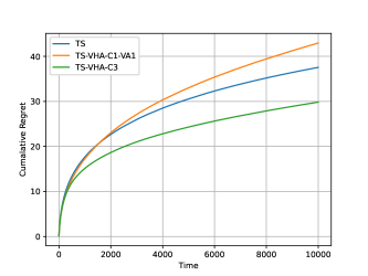
(a) 20 Arms
Refer to caption
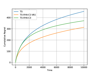
(b) 200 Arms
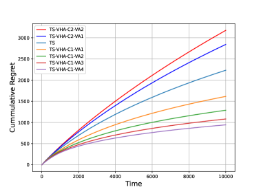
Figure 1: Gaussian bandit: Cumulative regret comparison of TS with TS-VHA-𝖢𝟣𝖢𝟣\mathsf{C1} and TS-VHA-𝖢𝟤𝖢𝟤\mathsf{C2}.

In this section, we present computational experiments that illustrate the potential benefits of TS-VHA. In the following, TS-VHA-𝖢𝟣𝖢𝟣\mathsf{C1}-VAn𝑛n and TS-VHA-𝖢𝟤𝖢𝟤\mathsf{C2}-VAn𝑛n denote TS-VHA with n𝑛n virtual helping agents, with combiner 𝖢𝟣𝖢𝟣\mathsf{C1} and 𝖢𝟤𝖢𝟤\mathsf{C2}, respectively. Note that, as per the notation introduced in Section 3, N1=n𝑁1𝑛N-1=n and TS corresponds to N=1𝑁1N=1 with identity function as the combiner.

5.1 Gaussian Bandits

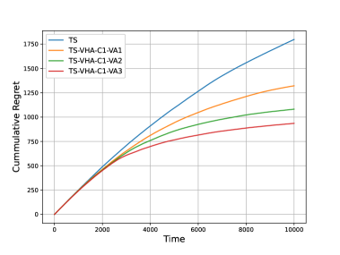
We evaluate the performance of TS-VHA-𝖢𝟣𝖢𝟣\mathsf{C1} and TS-VHA-𝖢𝟤𝖢𝟤\mathsf{C2} and compare it with TS for Gaussian bandits. First, we consider a 20 armed bandit problem with reward from arm i𝑖i modeled as 𝒩(μi,1)𝒩subscript𝜇𝑖1\mathcal{N}(\mu_{i},1), where the mean reward μisubscript𝜇𝑖\mu_{i} is independently sampled from 𝒰[0,1]𝒰01\mathcal{U}[0,1]. Fig. 1(a) shows the cumulative regret over 10000 time steps, averaged over 1000 independently sampled problem instances. Fig. 1(b) corresponds to a second Gaussian bandit problem with 200 arms, keeping all the other details same as that of the 20 armed bandit.

For TS-VHA-𝖢𝟣𝖢𝟣\mathsf{C1}-VAn𝑛n (TS-VHA-𝖢𝟤𝖢𝟤\mathsf{C2}-VAn𝑛n), exploitation (exploration) increases with n𝑛n, as compared to TS. As can be observed from the plots, increasing exploitation through TS-VHA-𝖢𝟣𝖢𝟣\mathsf{C1} improves the regret performance. It should be noted that having more exploitation might turn out to be counter-productive. As discussed in Section 3.1, as n𝑛n grows to a higher value, TS-VHA-𝖢𝟣𝖢𝟣\mathsf{C1}-VAn𝑛n starts behaving like the greedy algorithm. Observe that, in Fig. 1(a), TS-VHA-𝖢𝟣𝖢𝟣\mathsf{C1}-VA4 accumulates more regret and performs poorly relative to TS-VHA-𝖢𝟣𝖢𝟣\mathsf{C1}-VAn𝑛n, n=1,2,3𝑛123n=1,2,3.

Refer to caption
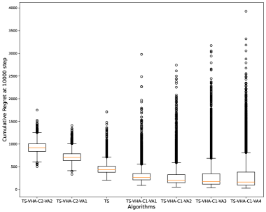
Figure 2: Variation in the cumulative regret with TS, TS-VHA-𝖢𝟣𝖢𝟣\mathsf{C1} and TS-VHA-𝖢𝟤𝖢𝟤\mathsf{C2} for Gaussian bandits.

Fig. 2 shows the distribution of final cumulative regret at the end of 10000 time steps, over 1000 runs, for a Gaussian bandit with 20 arms. Reward from arm i𝑖i is distributed as 𝒩(μi,1)𝒩subscript𝜇𝑖1\mathcal{N}(\mu_{i},1), where μi,i=1,,20formulae-sequencesubscript𝜇𝑖𝑖120\mu_{i},i=1,\ldots,20, is chosen by sampling independently from 𝒰[0,1]𝒰01\mathcal{U}[0,1] once at the beginning of the experiment and kept constant throughout the 1000 runs. TS-VHA-𝖢𝟣𝖢𝟣\mathsf{C1} has a higher variance in its final cumulative regret and is thus not suitable for risk-sensitive scenarios. On the other hand, TS-VHA-𝖢𝟤𝖢𝟤\mathsf{C2} results in a lower variance in its final cumulative regret and may be preferred in risk-averse applications.

5.2 Bernoulli Bandits
Refer to caption
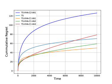
(a) 20 Arms
Refer to caption
(b) 200 Arms
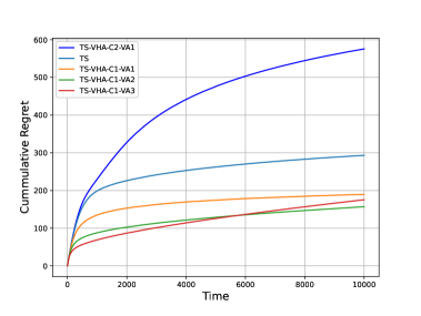
Figure 3: Bernoulli bandit: Cumulative regret comparison of TS with TS-VHA-𝖢𝟣𝖢𝟣\mathsf{C1} and TS-VHA-𝖢𝟤𝖢𝟤\mathsf{C2}.

We now evaluate the performance of TS-VHA over Bernoulli bandits, i.e., bandit problems with Bernoulli distributed rewards and Beta distribution as the prior.

5.2.1 Bernoulli Bandit with Randomized Mean Rewards

Similar to the Gaussian bandits discussed above, we consider two Bernoulli bandit problems, one with 20 arms and the other with 200 arms, with mean reward of each arm is independently sampled from 𝒰[0,1]𝒰01\mathcal{U}[0,1].

Fig. 3(a) and Fig. 3(b) shows the cumulative regret over 100000 time steps, averaged over 1000 independently sampled problem instances, for the 20 armed bandit and the 200 armed bandit, respectively.

5.2.2 Real World Datasets

Here, we show the effectiveness of TS-VHA-𝖢𝟣𝖢𝟣\mathsf{C1} on the real-world data sets Coupon-Purchase [25] and edX-Courses [26].
Refer to caption
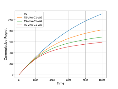
(a) Considering coupon purchase rate as the mean reward of each arm.
Refer to caption
(b) Considering coupon purchase rate multiplied by the normalized selling price as the mean reward of each arm.
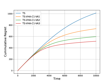
Figure 4: Bernoulli bandit problem with 142 arms, formulated using the Coupon-Purchase dataset.

The Coupon-Purchase dataset contains discount coupons applied to online purchases. From the dataset, we have considered only 142 coupons that correspond to products priced less than or equal to 200 price units and purchased by at least one customer (as in [27]). For these 142 coupons, we have extracted the purchase rate that lies within [0,0.3]00.3[0,0.3] and the final selling price normalized by 200 price units, which lies within (0,1]01(0,1]. With each coupon as an independent arm that (when played) generates a binary valued reward according to a Bernoulli distribution, we formulate two bandit problems. In the first one, the mean reward of an arm is equal to the corresponding coupon purchase rate and, in the second problem, the mean reward of each arm is equal to the coupon purchase rate multiplied by the corresponding selling price normalized by 200. By modeling the mean reward of each arm using a Beta distribution, we present the performance of TS and TS-VHA-𝖢𝟣𝖢𝟣\mathsf{C1}-VAn𝑛n, n=1,2,3𝑛123n=1,2,3, in Fig. 4(a) and Fig. 4(b), corresponding to the first and the second problem, respectively. As can be seen, TS-VHA with combiner 𝖢𝟣𝖢𝟣\mathsf{C1} helps achieving a lower cumulative regret for both the problems.
Refer to caption
(a) Considering the course certification rate as the mean reward of each arm.
Refer to caption
(b) Considering the course certification rate multiplied by the course participation rate as the mean reward of each arm.
Figure 5: Bernoulli bandit problem with 290 arms, formulated using the edX-Course datset.

The edX-Courses dataset contains information regarding 290 Harvard and MIT courses and, as in [28], we compute the normalized course participation rates (that lie within unit interval) through min-max normalization of the number of participants in each course and obtain the course certification rates by dividing the number of certified participants in each course by the number of course participants. We formulate two bandit problems by considering each course as an independent arm that returns a Bernoulli distributed reward. In the first problem, the mean reward of each arm is given by the course certification rate and in the second, course certification rate multiplied by the course participation rate is the mean reward.

With Beta distribution as the prior for the mean reward of each arm, Fig. 5(a) and Fig. 5(b) compare the cumulative regret performance of TS and and TS-VHA-𝖢𝟣𝖢𝟣\mathsf{C1}-VAn𝑛n, n=1,2,3𝑛123n=1,2,3, for the first and the second problem, respectively.
Refer to caption
(a) Deterministic bandit.
Refer to caption
(b) Bernoulli bandit
Refer to caption
(c) Independent Gaussian
Refer to caption
(d) Linear Gaussian
Figure 6: Time-sensitive Bandit Learning
Refer to caption
(a) Gaussian bandit with two arms. Mean rewards: 0.5, 0.25.
Refer to caption
(b) Bernoulli bandit with two arms. Mean rewards: 0.51, 0.5.
Figure 7: Best arm identification for two armed Bernoulli and Gaussian bandits.
Refer to caption
(a) Bernoulli bandit, 2 arms
Refer to caption
(b) Bernoulli bandit, 20 arms
Refer to caption
(c) Gaussian bandit, 2 arms
Refer to caption
(d) Gaussian bandit, 20 arms
Figure 8: Cumulative regret comparison of TS-VHA-𝖢𝟥𝖢𝟥\mathsf{C3} with TS and TS-VHA-𝖢𝟥𝖢𝟥\mathsf{C3}

5.3 Time-Sensitive Bandit Learning

Most of the bandit algorithms focus on learning the optimal arm (or, action). Often, especially for bandit problems having a very large set of arms, convergence to optimality may take a long time rendering them not useful in some practical applications. For example, in the case of a recommender system, the learning agent may be required to impress upon the users through its near optimal recommendations during the early interactions; Or, the learning agent may not have enough number of interactions with each user to converge onto perfect recommendations.

In [29], the authors have addressed the problem of learning near-optimal satisficing actions considering situations where the near term performance is more important than the performance over an asymptotically long time horizon, or, the optimal action is costly to learn relative to near-optimal actions. Satisficing Thompson Sampling (STS), proposed in [29], performs time-sensitive learning by modifying the Select action step of TS.

Recall that, in TS (i.e., Algorithm 1), θi(τ)subscript𝜃𝑖𝜏\theta_{i}(\tau) is the sample drawn from posterior of arm i𝑖i at time τ𝜏\tau, i(τ)𝑖𝜏i(\tau) is the index of arm played at time τ𝜏\tau and θi(τ)subscript𝜃𝑖𝜏\theta_{i(\tau)} is the expected reward of the arm played at time τ𝜏\tau. At each time step t𝑡t, STS identifies an ϵitalic-ϵ\epsilon-optimal action through the following Select action step.

Select action (in STS):

  • Let i(t)=argmaxiθi(t)𝑖𝑡subscript𝑖subscript𝜃𝑖𝑡i(t)=\arg\max_{i}\theta_{i}(t).

  • Let τ^=min{τ{1,,t1}:θi(τ)+ϵθi(t)}^𝜏:𝜏1𝑡1subscript𝜃𝑖𝜏italic-ϵsubscript𝜃𝑖𝑡{\hat{\tau}}=\min\{\tau\in\{1,\ldots,t-1\}:\theta_{i(\tau)}+\epsilon\geq\theta_{i(t)}\}.

  • If τ^^𝜏\hat{\tau} is not null, then i(t)=i(τ^)𝑖𝑡𝑖^𝜏i(t)=i(\hat{\tau}).

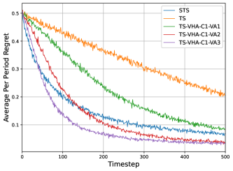
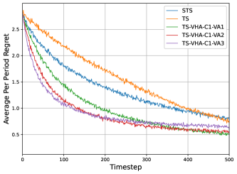
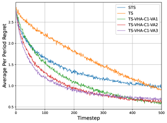
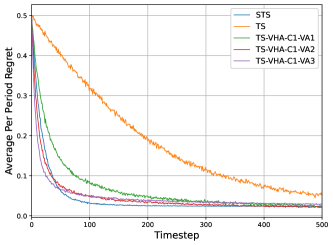
Essentially, at each time step t𝑡t, STS chooses to play an arm k𝑘k that has already been played in the past, as long as the estimate of the expected reward from arm k𝑘k is not lower than the estimate of the expected reward from an optimal arm (optimal at time t𝑡t as per the TS) by ϵitalic-ϵ\epsilon units. Thus, STS exploits more by re-using near-optimal satisficing arms rather than exploring un-used arms. With per period regret as the performance metric (that captures the time preference), the simulation experiments reported in [29] show that STS can significantly outperform TS when the optimal action is costly to learn relative to satisficing near-optimal actions. We consider four simulation experiments that are same as those considered in [29] and compare the performance of TS-VHA-𝖢𝟣𝖢𝟣\mathsf{C1} with that of STS and TS in Fig. 8. For all the four experiments, we compute the per period regret over 500 time steps, averaged over 5000 runs. Fig. 6(a) considers a deterministic bandit with 250 arms with mean reward of each arm sampled independently from 𝒰[0,1]𝒰01\mathcal{U}[0,1]. As every arm, when played, returns the reward equal to its mean reward, it is referred to as a deterministic bandit. Performance of TS-VHA-𝖢𝟣𝖢𝟣\mathsf{C1}-VA2 and TS-VHA-𝖢1𝖢1\mathsf{C}1-VA3 is very close to that of STS. Fig. 6(b) corresponds to a bandit that differs from that of Fig. 6(a) as follows: Whenever an arm is played, the observed reward is a Bernoulli random variable with success probability equal to the mean reward. Note that, in Fig. 6(a) and Fig. 6(b), we consider ϵ=0.05italic-ϵ0.05\epsilon=0.05 for the STS. It can be observed that TS-VHA-𝖢𝟣𝖢𝟣\mathsf{C1}-VA2 and TS-VHA-𝖢𝟣𝖢𝟣\mathsf{C1}-VA3 perform better than STS for time step values above (approximately) 150 and 50, respectively. Fig. 6(c) corresponds to a 250 armed Gaussian bandit with mean reward of each arm sampled independently from 𝒩(0,1)𝒩01\mathcal{N}(0,1); When an arm is played, the realized reward is the sum of the arm’s mean reward and an independent sample from 𝒩(0,1)𝒩01\mathcal{N}(0,1). Here, ϵ=0.5italic-ϵ0.5\epsilon=0.5 for the STS. Finally, we consider linear Gaussian bandit with 250 arms in Fig. 6(d). The mean rewards are given by the vector 𝐋𝜽250×1𝐋𝜽superscript2501\mathbf{L}\boldsymbol{\theta}\in\mathbb{R}^{250\times 1}, where 𝜽250×1𝜽superscript2501\boldsymbol{\theta}\in\mathbb{R}^{250\times 1} is sampled from 𝒩(0,𝐈)𝒩0𝐈\mathcal{N}(0,\mathbf{I}) and 𝐋250×250𝐋superscript250250\mathbf{L}\in\mathbb{R}^{250\times 250} is a random matrix with each row drawn independently and uniformly from the unit sphere. While 𝜽𝜽\boldsymbol{\theta} is unknown a priori, 𝐋𝐋\mathbf{L} is known before hand. When an arm is played the observed reward is the sum of the mean reward and an independent sample from 𝒩(0,2)𝒩02\mathcal{N}(0,2). As can be observed from Fig. 6(c) and Fig. 6(d), TS-VHA-𝖢𝟣𝖢𝟣\mathsf{C1} outperforms TS and STS for both independent Gaussian and Linear Gaussian bandits.

We think, the above simulation experiments only indicate that it might be interesting to investigate (and analyze) the TS-VHA-𝖢𝟣𝖢𝟣\mathsf{C1} from the aspect of time-sensitive learning.

5.4 Best Arm Identification

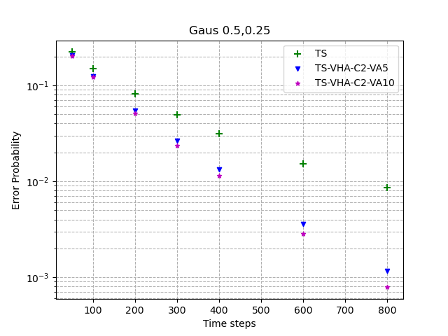
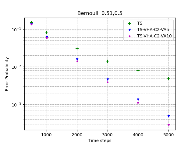
Next, we consider the fixed budget setting of the Best Arm Identification problem as discussed in [30]. The idea is to identify the best arm amongst all the bandit arms by playing them intelligently for a fixed number of time steps t𝑡t. The metric used to compare algorithms is the probability of error in identifying the best arm after the fixed time step t𝑡t.

TS can be utilized to solve this problem by designating the arm with the highest empirical mean after t𝑡t time steps as the best arm. However, TS performs poorly for this pure-exploration problem because of its high exploitative nature. Therefore, with the intention to increase the exploration in TS, we evaluate the applicability of TS-VHA-𝖢𝟤𝖢𝟤\mathsf{C2} in this scenario.

In Fig. 7, we consider the Bernoulli bandit as well as Gaussian bandit, each having two arms. The plots on the left and right have arms with mean rewards equal to (0.5,0.25)0.50.25(0.5,0.25) and (0.51,0.5)0.510.5(0.51,0.5), respectively. For both the scenarios, we observe that TS-VHA-𝖢𝟤𝖢𝟤\mathsf{C2} outperforms TS empirically.

5.5 Combiner 𝖢𝟥𝖢𝟥\mathsf{C3}

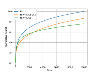
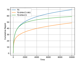
Finally, we evaluate the cumulative regret performance of Combiner 𝖢𝟥𝖢𝟥\mathsf{C3}, through simulations, for Bernoulli bandits and Gaussian bandits and compare its performance with TS and TS-VHA-𝖢𝟣𝖢𝟣\mathsf{C1}.

Similar to section 5-A and 5-B, we first evaluate the performance of 𝖢𝟥𝖢𝟥\mathsf{C3} on the randomized 20 arms case. As shown in Fig. 8(b) and Fig. 8(d), for both Gaussian and Bernoulli bandits, TS-VHA-𝖢𝟥𝖢𝟥\mathsf{C3} outperforms TS.

Next, we choose the same randomized scenario but with two arms in Fig. 8(a) and Fig. 8(c). In this case, 𝖢𝟥𝖢𝟥\mathsf{C3} outperforms both TS and TS-VHA-𝖢𝟣𝖢𝟣\mathsf{C1} significantly. Interestingly, for the Gaussian bandits, TS-VHA-𝖢𝟣𝖢𝟣\mathsf{C1} performs inferior to TS, suggesting that, in some cases, increasing exploitation from the beginning does not help in optimizing the cumulative regret. But, dynamically adjusting the amount of exploitation over time by 𝖢𝟥𝖢𝟥\mathsf{C3} provides superior performance. A mathematical analysis of the regret bound for 𝖢𝟥𝖢𝟥\mathsf{C3} would help gaining more insight into it.

6 Conclusion

We have proposed a general framework, Thompson Sampling with Virtual Helping Agents (TS-VHA), that combines samples drawn by the virtual agents to maneuver the exploration vs exploitation tradeoff in Thompson Sampling. Based on this framework, we developed two linear combiners (TS-VHA-𝖢𝟣𝖢𝟣\mathsf{C1} and TS-VHA-𝖢𝟤𝖢𝟤\mathsf{C2}) and analysed theoretically their cumulative regret performance on Gaussian Bandits. Moreover, we showed their empirical efficacy on both Gaussian and Bernoulli bandits for multiple metrics: cumulative regret, best-arm identification and time-sensitive learning. We defer the analysis of the regret bounds on these metrics for our future work. To exhibit the broad scope of the framework, we also put forth a nonlinear combiner TS-VHA-𝖢𝟥𝖢𝟥\mathsf{C3} that dynamically tunes the amount of exploration/exploitation and offers superior empirical performance. It would be interesting to experiment and devise more sophisticated combiners. TS-VHA can be applied wherever Thompson Sampling can be applied and we leave extending TS-VHA (along with designing combiners) for contextual bandits, non-stationary bandits and restless bandits for future work. Finally, exploring the usage of neural networks in developing combiners would be an exciting avenue for future work.

\appendices

7 Inequalities used in the regret analysis

Inequality 1.

(Chernoff-Hoeffding Bound) Let X1,,Xnsubscript𝑋1subscript𝑋𝑛X_{1},\ldots,X_{n} be independent 0 - 1 r.v.s with E[Xi]=pi𝐸delimited-[]subscript𝑋𝑖subscript𝑝𝑖E[X_{i}]=p_{i} (not necessarily equal). Let X=1niXi𝑋1𝑛subscript𝑖subscript𝑋𝑖X=\frac{1}{n}\sum_{i}X_{i}, μ=E[X]=1ni=1npi𝜇𝐸delimited-[]𝑋1𝑛superscriptsubscript𝑖1𝑛subscript𝑝𝑖\mu=E[X]=\frac{1}{n}\sum_{i=1}^{n}p_{i}. Then, for any 0<λ<1μ0𝜆1𝜇0<\lambda<1-\mu,

Pr(Xμ+λ)end(μ+λ,μ),Pr𝑋𝜇𝜆superscript𝑒𝑛𝑑𝜇𝜆𝜇\text{Pr}(X\geq\mu+\lambda)\leq e^{-nd(\mu+\lambda,\mu)},

and for any 0<λ<μ0𝜆𝜇0<\lambda<\mu,

Pr(Xμλ)end(μλ,μ),Pr𝑋𝜇𝜆superscript𝑒𝑛𝑑𝜇𝜆𝜇\text{Pr}(X\geq\mu-\lambda)\leq e^{-nd(\mu-\lambda,\mu)},

where d(a,b)=alnab+(1a)ln1a1b𝑑𝑎𝑏𝑎𝑎𝑏1𝑎1𝑎1𝑏d(a,b)=a\ln{\frac{a}{b}+(1-a)\ln{\frac{1-a}{1-b}}}

Inequality 2.

(Chernoff-Hoeffding Bound) Let X1,,Xnsubscript𝑋1subscript𝑋𝑛X_{1},\ldots,X_{n} be random variables with common range [0,1]01[0,1] and such that 𝔼[Xt|X1,,Xt1]=μ𝔼delimited-[]conditionalsubscript𝑋𝑡subscript𝑋1subscript𝑋𝑡1𝜇\mathbb{E}[X_{t}|X_{1},\ldots,X_{t-1}]=\mu. Let Sn=i=1nXisubscript𝑆𝑛superscriptsubscript𝑖1𝑛subscript𝑋𝑖S_{n}=\sum_{i=1}^{n}X_{i}. Then, for all a0𝑎0a\geq 0,

Pr(Snnμ+a)e2a2/n,Prsubscript𝑆𝑛𝑛𝜇𝑎superscript𝑒2superscript𝑎2𝑛\text{Pr}(S_{n}\geq n\mu+a)\leq e^{-2a^{2}/n},

and

Pr(Snnμa)e2a2/n.Prsubscript𝑆𝑛𝑛𝜇𝑎superscript𝑒2superscript𝑎2𝑛\text{Pr}(S_{n}\leq n\mu-a)\leq e^{-2a^{2}/n}.

The following inequalities can be derived for a Gaussian random variable from Formula 7.1.137.1.137.1.13 in [24].

Inequality 3.

For a Gaussian distributed random variable Z𝑍Z with mean m𝑚m and variance σ2superscript𝜎2\sigma^{2},

Pr(Z>m+xσ)x2π(x2+1)ex2/2.Pr𝑍𝑚𝑥𝜎𝑥2𝜋superscript𝑥21superscript𝑒superscript𝑥22\text{Pr}(Z>m+x\sigma)\geq\frac{x}{\sqrt{2\pi}(x^{2}+1)}e^{-x^{2}/2}.
Inequality 4.

For a Gaussian distributed random variable Z𝑍Z with mean m𝑚m and variance σ2superscript𝜎2\sigma^{2}, for any z𝑧z,

14πe7z2/2<Pr(|Zm|>zσ)12ez2/2.14𝜋superscript𝑒7superscript𝑧22𝑃𝑟𝑍𝑚𝑧𝜎12superscript𝑒superscript𝑧22\frac{1}{4\sqrt{\pi}}e^{-7z^{2}/2}<Pr(|Z-m|>z\sigma)\leq\frac{1}{2}e^{-z^{2}/2}.
Inequality 5.

Let Sn=i=1n1ipsubscript𝑆𝑛superscriptsubscript𝑖1𝑛1superscript𝑖𝑝S_{n}=\sum_{i=1}^{n}\frac{1}{i^{p}}. Then for 0<p<10𝑝10<p<1 from [31],

Sn<1+(n+1)1p11psubscript𝑆𝑛1superscript𝑛11𝑝11𝑝S_{n}<1+\frac{(n+1)^{1-p}-1}{1-p}

8 Proof of Lemma 1

Recall that θi(t)𝒩(μ^i(t),1γ(ki(t)+1))similar-tosubscript𝜃𝑖𝑡𝒩subscript^𝜇𝑖𝑡1𝛾subscript𝑘𝑖𝑡1\theta_{i}(t)\sim\mathcal{N}\left(\hat{\mu}_{i}(t),\frac{1}{\gamma(k_{i}(t)+1)}\right), xi=μi+Δi3subscript𝑥𝑖subscript𝜇𝑖subscriptΔ𝑖3x_{i}=\mu_{i}+\frac{\Delta_{i}}{3}, yi=μ1Δi3subscript𝑦𝑖subscript𝜇1subscriptΔ𝑖3y_{i}=\mu_{1}-\frac{\Delta_{i}}{3} and Li(T)=2lnTΔi2γ(yixi)2subscript𝐿𝑖𝑇2𝑇superscriptsubscriptΔ𝑖2𝛾superscriptsubscript𝑦𝑖subscript𝑥𝑖2L_{i}(T)=\frac{2\ln{T\Delta_{i}^{2}}}{\gamma(y_{i}-x_{i})^{2}}. Given τksubscriptsubscript𝜏𝑘\mathcal{F}_{\tau_{k}}, let ΘksubscriptΘ𝑘\Theta_{k} denote a Gaussian random variable distributed as 𝒩(μ^1(τk+1),1γ(k+1))𝒩subscript^𝜇1subscript𝜏𝑘11𝛾𝑘1\mathcal{N}\left(\hat{\mu}_{1}(\tau_{k}+1),\frac{1}{\gamma(k+1)}\right). For convenience, we denote μ^1(τk+1)subscript^𝜇1subscript𝜏𝑘1\hat{\mu}_{1}(\tau_{k}+1) with μ^1subscript^𝜇1\hat{\mu}_{1} in the following. Let Gksubscript𝐺𝑘G_{k} be the geometric random variable representing the number of consecutive independent trials until a sample of ΘksubscriptΘ𝑘\Theta_{k} becomes greater than yisubscript𝑦𝑖y_{i}. Using ΘksubscriptΘ𝑘\Theta_{k} and Definition 6, we can write pi,τk+1=Pr(Θk>yi|τk)subscript𝑝𝑖subscript𝜏𝑘1PrsubscriptΘ𝑘conditionalsubscript𝑦𝑖subscriptsubscript𝜏𝑘p_{i,\tau_{k}+1}=\text{Pr}(\Theta_{k}>y_{i}|\mathcal{F}_{\tau_{k}}), and

𝔼[(1pi,τk+1)pi,τk+1]=𝔼[𝔼[Gk|τk]]=𝔼[Gk].𝔼delimited-[]1subscript𝑝𝑖subscript𝜏𝑘1subscript𝑝𝑖subscript𝜏𝑘1𝔼delimited-[]𝔼delimited-[]conditionalsubscript𝐺𝑘subscriptsubscript𝜏𝑘𝔼delimited-[]subscript𝐺𝑘\mathbb{E}\left[\frac{(1-p_{i,\tau_{k}+1})}{p_{i,\tau_{k}+1}}\right]=\mathbb{E}[\mathbb{E}[G_{k}|\ \mathcal{F}_{\tau_{k}}]]=\mathbb{E}[G_{k}].

Therefore,

k=0T1𝔼[(1pi,τk+1)pi,τk+1]=k=04Li(T)1𝔼[Gk]Sum (21a)+k=4Li(T)T1𝔼[Gk]Sum (21b)superscriptsubscript𝑘0𝑇1𝔼delimited-[]1subscript𝑝𝑖subscript𝜏𝑘1subscript𝑝𝑖subscript𝜏𝑘1subscriptsuperscriptsubscript𝑘04subscript𝐿𝑖𝑇1𝔼delimited-[]subscript𝐺𝑘Sum (21a)subscriptsuperscriptsubscript𝑘4subscript𝐿𝑖𝑇𝑇1𝔼delimited-[]subscript𝐺𝑘Sum (21b)\sum_{k=0}^{T-1}\mathbb{E}\left[\frac{(1-p_{i,\tau_{k}+1})}{p_{i,\tau_{k}+1}}\right]=\underbrace{\sum_{k=0}^{4L_{i}(T)-1}\mathbb{E}[G_{k}]}_{\text{Sum (\ref{eq:sums}a)}}+\underbrace{\sum_{k=4L_{i}(T)}^{T-1}\mathbb{E}[G_{k}]}_{\text{Sum (\ref{eq:sums}b)}} (21)

We will now bound Sum (21a), first term on the RHS of (21). Let z=lnrβ𝑧superscript𝑟𝛽z=\sqrt{\ln{r^{\beta}}}, where r1𝑟1r\geq 1 is an integer, β[1,2)𝛽12\beta\in[1,2), and let Mrsubscript𝑀𝑟M_{r} denote the maximum of r𝑟r independent samples of ΘksubscriptΘ𝑘\Theta_{k}.

Pr(Gk<r)Prsubscript𝐺𝑘𝑟\displaystyle\text{Pr}(G_{k}<r) Pr(Mr>yi)absentPrsubscript𝑀𝑟subscript𝑦𝑖\displaystyle\geq\text{Pr}(M_{r}>y_{i})
Pr(Mr>μ^1+zγ(k+1)>yi)absentPrsubscript𝑀𝑟subscript^𝜇1𝑧𝛾𝑘1subscript𝑦𝑖\displaystyle\geq\text{Pr}\left(M_{r}>\hat{\mu}_{1}+\frac{z}{\sqrt{\gamma(k+1)}}>y_{i}\right)
=𝔼[𝔼[Mr>η>yiτk]]absent𝔼delimited-[]𝔼delimited-[]subscript𝑀𝑟𝜂conditionalsubscript𝑦𝑖subscriptsubscript𝜏𝑘\displaystyle=\mathbb{E}\left[\mathbb{E}\left[M_{r}>\eta>y_{i}\mid\mathcal{F}_{\tau_{k}}\right]\right]
=𝔼[I(η>yi)Pr(Mr>ητk)],absent𝔼delimited-[]𝐼𝜂subscript𝑦𝑖Prsubscript𝑀𝑟conditional𝜂subscriptsubscript𝜏𝑘\displaystyle=\mathbb{E}\left[I\left(\eta>y_{i}\right)\text{Pr}\left(M_{r}>\eta\mid\mathcal{F}_{\tau_{k}}\right)\right], (22)

where η=μ^1+zγ(k+1)𝜂subscript^𝜇1𝑧𝛾𝑘1\eta=\hat{\mu}_{1}+\frac{z}{\sqrt{\gamma(k+1)}}. Since Θk𝒩(μ^1,1γ(k+1))similar-tosubscriptΘ𝑘𝒩subscript^𝜇11𝛾𝑘1\Theta_{k}\sim\mathcal{N}\left(\hat{\mu}_{1},\frac{1}{\gamma(k+1)}\right), using Inequality 3, we can write

Pr(Mr>η|τk=Fτk)\displaystyle\text{Pr}\left(M_{r}>\eta\;\middle|\;\mathcal{F}_{\tau_{k}}=F_{\tau_{k}}\right) 1(112πzz2+1ez22)rabsent1superscript112𝜋𝑧superscript𝑧21superscript𝑒superscript𝑧22𝑟\displaystyle\geq 1-\left(1-\frac{1}{\sqrt{2\pi}}\frac{z}{z^{2}+1}e^{\frac{-z^{2}}{2}}\right)^{r}
1er1β22βπlnr.absent1superscript𝑒superscript𝑟1𝛽22𝛽𝜋𝑟\displaystyle\geq 1-e^{-\frac{r^{1-\frac{\beta}{2}}}{\sqrt{2\beta\pi\ln{r}}}}. (23)

Note that Fτksubscript𝐹subscript𝜏𝑘F_{\tau_{k}} is any realization of τksubscriptsubscript𝜏𝑘\mathcal{F}_{\tau_{k}}. As β[1,2)𝛽12\beta\in[1,2), there exists a number h(β)>0𝛽subscriptabsent0h(\beta)\in\mathbb{R}_{>0} such that er1β22βπlnr1r2superscript𝑒superscript𝑟1𝛽22𝛽𝜋𝑟1superscript𝑟2e^{-\frac{r^{1-\frac{\beta}{2}}}{\sqrt{2\beta\pi\ln{r}}}}\leq\frac{1}{r^{2}} for rh(β)𝑟𝛽r\geq h(\beta). Hence, for any rh(β)𝑟𝛽r\geq h(\beta) and any γ>0𝛾0\gamma>0,

Pr(Mr>η|τk=Fτk)11r2\text{Pr}\left(M_{r}>\eta\;\middle|\;\mathcal{F}_{\tau_{k}}=F_{\tau_{k}}\right)\geq 1-\frac{1}{r^{2}} (24)

On substituting (24) in (22) we get, for any rh(β)𝑟𝛽r\geq h(\beta),

Pr(Gk<r)Prsubscript𝐺𝑘𝑟\displaystyle\text{Pr}(G_{k}<r) 𝔼[I(ηyi)(11r2)]absent𝔼delimited-[]𝐼𝜂subscript𝑦𝑖11superscript𝑟2\displaystyle\geq\mathbb{E}\left[I\left(\eta\geq y_{i}\right)\left(1-\frac{1}{r^{2}}\right)\right]
=(11r2)Pr(ηyi)absent11superscript𝑟2Pr𝜂subscript𝑦𝑖\displaystyle=\left(1-\frac{1}{r^{2}}\right)\text{Pr}(\eta\geq y_{i}) (25)

We will now find a lower bound on Pr(ηyi)Pr𝜂subscript𝑦𝑖\text{Pr}(\eta\geq y_{i}).

Pr(ηyi)=Pr(μ^1+zγ(k+1)μ1Δi3)=Pr(μ^1+1k+1μ1(Δi3+zγ(k+1)1k+1))Pr𝜂subscript𝑦𝑖Prsubscript^𝜇1𝑧𝛾𝑘1subscript𝜇1subscriptΔ𝑖3Prsubscript^𝜇11𝑘1subscript𝜇1subscriptΔ𝑖3𝑧𝛾𝑘11𝑘1\text{Pr}(\eta\geq y_{i})=\text{Pr}\left(\hat{\mu}_{1}+\frac{z}{\sqrt{\gamma(k+1)}}\geq\mu_{1}-\frac{\Delta_{i}}{3}\right)=\\ \text{Pr}\left(\hat{\mu}_{1}+\frac{1}{k+1}\geq\mu_{1}-\left(\frac{\Delta_{i}}{3}+\frac{z}{\sqrt{\gamma(k+1)}}-\frac{1}{k+1}\right)\right) (26)

1k+11𝑘1\frac{1}{k+1} was added to μ^1subscript^𝜇1\hat{\mu}_{1} to account for the fact that μ^1subscript^𝜇1\hat{\mu}_{1} is not the average of the past k𝑘k observations, but it is the sum of the past k𝑘k observations divided by (k+1)𝑘1(k+1). Applying Inequality 2 to (26),

Pr(ηyi)1e2(Δi(k+1)3+zγ1k+1)2.Pr𝜂subscript𝑦𝑖1superscript𝑒2superscriptsubscriptΔ𝑖𝑘13𝑧𝛾1𝑘12\text{Pr}(\eta\geq y_{i})\geq 1-e^{-2\left(\frac{\Delta_{i}\sqrt{(k+1)}}{3}+\frac{z}{\sqrt{\gamma}}-\frac{1}{\sqrt{k+1}}\right)^{2}}. (27)

Substituting (27) back into (25), for any rh(β)𝑟𝛽r\geq h(\beta),

Pr(Gk<r)Prsubscript𝐺𝑘𝑟\displaystyle\text{Pr}(G_{k}<r) (11r2)(1e2(Δi(k+1)3+zγ1k+1)2)absent11superscript𝑟21superscript𝑒2superscriptsubscriptΔ𝑖𝑘13𝑧𝛾1𝑘12\displaystyle\geq\left(1-\frac{1}{r^{2}}\right)\left(1-e^{-2\left(\frac{\Delta_{i}\sqrt{(k+1)}}{3}+\frac{z}{\sqrt{\gamma}}-\frac{1}{\sqrt{k+1}}\right)^{2}}\right)
11r2e2(Δi(k+1)3+zγ1k+1)2.absent11superscript𝑟2superscript𝑒2superscriptsubscriptΔ𝑖𝑘13𝑧𝛾1𝑘12\displaystyle\geq 1-\frac{1}{r^{2}}-e^{-2\left(\frac{\Delta_{i}\sqrt{(k+1)}}{3}+\frac{z}{\sqrt{\gamma}}-\frac{1}{\sqrt{k+1}}\right)^{2}}. (28)

This leads us to

k=04Li(T)1𝔼[Gk]=k=04Li(T)1r=0TPr(Gkr)k=04Li(T)1r=0T(1r2+e2(Δi(k+1)3+zγ1k+1)2)superscriptsubscript𝑘04subscript𝐿𝑖𝑇1𝔼delimited-[]subscript𝐺𝑘superscriptsubscript𝑘04subscript𝐿𝑖𝑇1superscriptsubscript𝑟0𝑇Prsubscript𝐺𝑘𝑟superscriptsubscript𝑘04subscript𝐿𝑖𝑇1superscriptsubscript𝑟0𝑇1superscript𝑟2superscript𝑒2superscriptsubscriptΔ𝑖𝑘13𝑧𝛾1𝑘12\sum_{k=0}^{4L_{i}(T)-1}\mathbb{E}[G_{k}]=\sum_{k=0}^{4L_{i}(T)-1}\sum_{r=0}^{T}\text{Pr}(G_{k}\geq r)\\ \leq\sum_{k=0}^{\small{4L_{i}(T)-1}}\sum_{r=0}^{T}\left(\frac{1}{r^{2}}\right.\\ +\left.e^{-2\left(\frac{\Delta_{i}\sqrt{(k+1)}}{3}+\frac{z}{\sqrt{\gamma}}-\frac{1}{\sqrt{k+1}}\right)^{2}}\right) (29)

First term on the RHS in (29) can be upper bounded as follows.

k=04Li(T)1(r=0T1r2)superscriptsubscript𝑘04subscript𝐿𝑖𝑇1superscriptsubscript𝑟0𝑇1superscript𝑟2\displaystyle\sum_{k=0}^{4L_{i}(T)-1}\left(\sum_{r=0}^{T}\frac{1}{r^{2}}\right) k=04Li(T)1(h(β)+rh(β)1r2)absentsuperscriptsubscript𝑘04subscript𝐿𝑖𝑇1𝛽subscript𝑟𝛽1superscript𝑟2\displaystyle\leq\sum_{k=0}^{4L_{i}(T)-1}\left(h(\beta)+\sum_{r\geq h(\beta)}\frac{1}{r^{2}}\right)
k=04Li(T)1(h(β)+ζ(2))absentsuperscriptsubscript𝑘04subscript𝐿𝑖𝑇1𝛽𝜁2\displaystyle\leq\sum_{k=0}^{4L_{i}(T)-1}\left(h(\beta)+\zeta(2)\right)
(h(β)+ζ(2))4Li(T),absent𝛽𝜁24subscript𝐿𝑖𝑇\displaystyle\leq(h(\beta)+\zeta(2))4L_{i}(T), (30)

where ζ𝜁\zeta is the Riemann zeta function. Next, we consider the second term on the RHS of (29) and use k=k+1superscript𝑘𝑘1k^{\prime}=k+1 for convenience.

k=14Li(T)r=0Te2(Δik3+βlnrγ1k)2superscriptsubscriptsuperscript𝑘14subscript𝐿𝑖𝑇superscriptsubscript𝑟0𝑇superscript𝑒2superscriptsubscriptΔ𝑖superscript𝑘3𝛽𝑟𝛾1superscript𝑘2\displaystyle\sum_{k^{\prime}=1}^{\small{4L_{i}(T)}}\sum_{r=0}^{T}e^{-2\left(\frac{\Delta_{i}\sqrt{k^{\prime}}}{3}+\frac{\sqrt{\beta\ln{r}}}{\sqrt{\gamma}}-\frac{1}{\sqrt{k^{\prime}}}\right)^{2}}
=r=0Tk=14Li(T)e2(Δik3+βlnrγ)2e2ke4(βlnrkγ)e4Δi3absentsuperscriptsubscript𝑟0𝑇superscriptsubscriptsuperscript𝑘14subscript𝐿𝑖𝑇superscript𝑒2superscriptsubscriptΔ𝑖superscript𝑘3𝛽𝑟𝛾2superscript𝑒2superscript𝑘superscript𝑒4𝛽𝑟superscript𝑘𝛾superscript𝑒4subscriptΔ𝑖3\displaystyle=\sum_{r=0}^{T}\sum_{k^{\prime}=1}^{\small{4L_{i}(T)}}e^{-2\left(\frac{\Delta_{i}\sqrt{k^{\prime}}}{3}+\sqrt{\frac{\beta\ln{r}}{\gamma}}\right)^{2}}e^{\frac{-2}{k^{\prime}}}e^{4\left(\sqrt{\frac{\beta\ln{r}}{k^{\prime}\gamma}}\right)}e^{\frac{4\Delta_{i}}{3}}
r=0Tk=14Li(T)e2(Δik3+βlnrγ)2e4(βlnrkγ)e4Δi3absentsuperscriptsubscript𝑟0𝑇superscriptsubscriptsuperscript𝑘14subscript𝐿𝑖𝑇superscript𝑒2superscriptsubscriptΔ𝑖superscript𝑘3𝛽𝑟𝛾2superscript𝑒4𝛽𝑟superscript𝑘𝛾superscript𝑒4subscriptΔ𝑖3\displaystyle\leq\sum_{r=0}^{T}\sum_{k^{\prime}=1}^{\small{4L_{i}(T)}}e^{-2\left(\frac{\Delta_{i}\sqrt{k^{\prime}}}{3}+\sqrt{\frac{\beta\ln{r}}{\gamma}}\right)^{2}}e^{4\left(\sqrt{\frac{\beta\ln{r}}{k^{\prime}\gamma}}\right)}e^{\frac{4\Delta_{i}}{3}}
=r=0Tk=14Li(T)e2βlnrγe2Δi2k9e4Δi3βklnrγe4(βlnrγk)e4Δi3absentsuperscriptsubscript𝑟0𝑇superscriptsubscriptsuperscript𝑘14subscript𝐿𝑖𝑇superscript𝑒2𝛽𝑟𝛾superscript𝑒2superscriptsubscriptΔ𝑖2superscript𝑘9superscript𝑒4subscriptΔ𝑖3𝛽superscript𝑘𝑟𝛾superscript𝑒4𝛽𝑟𝛾superscript𝑘superscript𝑒4subscriptΔ𝑖3\displaystyle=\sum_{r=0}^{T}\sum_{k^{\prime}=1}^{\small{4L_{i}(T)}}e^{\frac{-2\beta\ln{r}}{\gamma}}e^{\frac{-2\Delta_{i}^{2}k^{\prime}}{9}}e^{\frac{-4\Delta_{i}}{3}\sqrt{\frac{\beta k^{\prime}\ln{r}}{\gamma}}}e^{4\left(\sqrt{\frac{\beta\ln{r}}{\gamma k^{\prime}}}\right)}e^{\frac{4\Delta_{i}}{3}}
(a)r=0Te2βlnrγe4(βlnrγ(1Δi3))e4Δi3k=14Li(T)e2Δi2k9𝑎superscriptsubscript𝑟0𝑇superscript𝑒2𝛽𝑟𝛾superscript𝑒4𝛽𝑟𝛾1subscriptΔ𝑖3superscript𝑒4subscriptΔ𝑖3superscriptsubscriptsuperscript𝑘14subscript𝐿𝑖𝑇superscript𝑒2superscriptsubscriptΔ𝑖2superscript𝑘9\displaystyle\overset{(a)}{\leq}\sum_{r=0}^{T}e^{\frac{-2\beta\ln{r}}{\gamma}}e^{4\left(\sqrt{\frac{\beta\ln{r}}{\gamma}}\left(1-\frac{\Delta_{i}}{3}\right)\right)}e^{\frac{4\Delta_{i}}{3}}\sum_{k^{\prime}=1}^{\small{4L_{i}(T)}}e^{\frac{-2\Delta_{i}^{2}k^{\prime}}{9}}
r=0Te2βlnrγe4(βlnrγ(1Δi3))e2Δi31e(2Δi291)absentsuperscriptsubscript𝑟0𝑇superscript𝑒2𝛽𝑟𝛾superscript𝑒4𝛽𝑟𝛾1subscriptΔ𝑖3superscript𝑒2subscriptΔ𝑖31superscript𝑒2superscriptsubscriptΔ𝑖291\displaystyle\overset{}{\leq}\sum_{r=0}^{T}e^{\frac{-2\beta\ln{r}}{\gamma}}e^{4\left(\sqrt{\frac{\beta\ln{r}}{\gamma}}\left(1-\frac{\Delta_{i}}{3}\right)\right)}e^{\frac{2\Delta_{i}}{3}}\frac{1}{e^{(\frac{2\Delta_{i}^{2}}{9}-1)}}
=(b)r=0Tcr2βγe4(βlnrγ(1Δi3))𝑏superscriptsubscript𝑟0𝑇superscript𝑐superscript𝑟2𝛽𝛾superscript𝑒4𝛽𝑟𝛾1subscriptΔ𝑖3\displaystyle\overset{(b)}{=}\sum_{r=0}^{T}\frac{c^{\prime}}{r^{\frac{2\beta}{\gamma}}}e^{4\left(\sqrt{\frac{\beta\ln{r}}{\gamma}}\left(1-\frac{\Delta_{i}}{3}\right)\right)} (31)

(a)𝑎(a) is due to the fact that max(e4Δi3(βklnrγ)e4(βlnrγk))=e4(βlnrγ(1Δi3))superscript𝑒4subscriptΔ𝑖3𝛽superscript𝑘𝑟𝛾superscript𝑒4𝛽𝑟𝛾superscript𝑘superscript𝑒4𝛽𝑟𝛾1subscriptΔ𝑖3\max\left(e^{\frac{-4\Delta_{i}}{3}\left(\sqrt{\frac{\beta k^{\prime}\ln{r}}{\gamma}}\right)}e^{4\left(\sqrt{\frac{\beta\ln{r}}{\gamma k^{\prime}}}\right)}\right)=e^{4\left(\sqrt{\frac{\beta\ln{r}}{\gamma}}\left(1-\frac{\Delta_{i}}{3}\right)\right)} at k=1superscript𝑘1k^{\prime}=1. In (b)𝑏(b), c=e4Δi3/(e2Δi291)superscript𝑐superscript𝑒4subscriptΔ𝑖3superscript𝑒2superscriptsubscriptΔ𝑖291c^{\prime}=e^{\frac{4\Delta_{i}}{3}}/(e^{\frac{2\Delta_{i}^{2}}{9}-1}). For any ϵ>0italic-ϵ0\epsilon>0, there exists a number g(ϵg(\epsilon) such that e4lnrγ(1Δi3)r2βγ1r2βγϵsuperscript𝑒4𝑟𝛾1subscriptΔ𝑖3superscript𝑟2𝛽𝛾1superscript𝑟2𝛽𝛾italic-ϵ\frac{e^{4\sqrt{\frac{\ln{r}}{\gamma}}\left(1-\frac{\Delta_{i}}{3}\right)}}{r^{\frac{2\beta}{\gamma}}}\leq\frac{1}{r^{\frac{2\beta}{\gamma}-\epsilon}} for rg(ϵ)𝑟𝑔italic-ϵr\geq g(\epsilon). Hence, for β[1,2)𝛽12\beta\in[1,2), γ>0𝛾0\gamma>0, ϵ>0italic-ϵ0\epsilon>0 and rg(ϵ)𝑟𝑔italic-ϵr\geq g(\epsilon),

k=14Li(T)r=0Te2(Δik3+βlnrγ1k)2r=0Tcr2βγϵsuperscriptsubscriptsuperscript𝑘14subscript𝐿𝑖𝑇superscriptsubscript𝑟0𝑇superscript𝑒2superscriptsubscriptΔ𝑖superscript𝑘3𝛽𝑟𝛾1superscript𝑘2superscriptsubscript𝑟0𝑇superscript𝑐superscript𝑟2𝛽𝛾italic-ϵ\sum_{k^{\prime}=1}^{\small{4L_{i}(T)}}\sum_{r=0}^{T}e^{-2\left(\frac{\Delta_{i}\sqrt{k^{\prime}}}{3}+\frac{\sqrt{\beta\ln{r}}}{\sqrt{\gamma}}-\frac{1}{\sqrt{k^{\prime}}}\right)^{2}}\leq\sum_{r=0}^{T}\frac{c^{\prime}}{r^{\frac{2\beta}{\gamma}-\epsilon}} (32)

We will analyze (32) separately for γ(0,4)𝛾04\gamma\in(0,4) and γ4𝛾4\gamma\geq 4.

For any value of γ(0,4)𝛾04\gamma\in(0,4), we choose β[1,2)𝛽12\beta\in[1,2) such that γ<2β𝛾2𝛽\gamma<2\beta. Then, we select ϵ>0italic-ϵ0\epsilon>0 to have 2βγϵ>12𝛽𝛾italic-ϵ1\frac{2\beta}{\gamma}-\epsilon>1. Thus, for γ(0,4)𝛾04\gamma\in(0,4), (32) can be further simplified as,

k=14Li(T)r=0Te2(Δik3+βlnrγ1k)2r=0Tcr2βγϵsuperscriptsubscriptsuperscript𝑘14subscript𝐿𝑖𝑇superscriptsubscript𝑟0𝑇superscript𝑒2superscriptsubscriptΔ𝑖superscript𝑘3𝛽𝑟𝛾1superscript𝑘2superscriptsubscript𝑟0𝑇superscript𝑐superscript𝑟2𝛽𝛾italic-ϵ\displaystyle\sum_{k^{\prime}=1}^{\small{4L_{i}(T)}}\sum_{r=0}^{T}e^{-2\left(\frac{\Delta_{i}\sqrt{k^{\prime}}}{3}+\frac{\sqrt{\beta\ln{r}}}{\sqrt{\gamma}}-\frac{1}{\sqrt{k^{\prime}}}\right)^{2}}\leq\sum_{r=0}^{T}\frac{c^{\prime}}{r^{\frac{2\beta}{\gamma}-\epsilon}}
cg(ϵ)+rcg(ϵ)cr2βγϵabsentsuperscript𝑐𝑔italic-ϵsubscript𝑟superscript𝑐𝑔italic-ϵsuperscript𝑐superscript𝑟2𝛽𝛾italic-ϵ\displaystyle\leq c^{\prime}g(\epsilon)+\sum_{r\geq c^{\prime}g(\epsilon)}\frac{c^{\prime}}{r^{\frac{2\beta}{\gamma}-\epsilon}}
c(g(ϵ)+ζ(2βγϵ))absentsuperscript𝑐𝑔italic-ϵ𝜁2𝛽𝛾italic-ϵ\displaystyle\leq c^{\prime}\left(g(\epsilon)+\zeta\left(\frac{2\beta}{\gamma}-\epsilon\right)\right) (33)

Since 2βγϵ>12𝛽𝛾italic-ϵ1\frac{2\beta}{\gamma}-\epsilon>1 and ζ𝜁\zeta is the Riemann zeta function, ζ(2βγϵ)𝜁2𝛽𝛾italic-ϵ\zeta\left(\frac{2\beta}{\gamma}-\epsilon\right) is a finite number.

On the other hand, for γ4𝛾4\gamma\geq 4, 2βγϵ<12𝛽𝛾italic-ϵ1\frac{2\beta}{\gamma}-\epsilon<1 for any choice of β𝛽\beta and ϵitalic-ϵ\epsilon. If we fix β[1,2)𝛽12\beta\in[1,2) and ϵ>0italic-ϵ0\epsilon>0 such that 2βγϵ>02𝛽𝛾italic-ϵ0\frac{2\beta}{\gamma}-\epsilon>0 (32) results in,

k=14Li(T)r=0Tsuperscriptsubscriptsuperscript𝑘14subscript𝐿𝑖𝑇superscriptsubscript𝑟0𝑇\displaystyle\sum_{k^{\prime}=1}^{\small{4L_{i}(T)}}\sum_{r=0}^{T} e2(Δik3+βlnrγ1k)2superscript𝑒2superscriptsubscriptΔ𝑖superscript𝑘3𝛽𝑟𝛾1superscript𝑘2\displaystyle e^{-2\left(\frac{\Delta_{i}\sqrt{k^{\prime}}}{3}+\frac{\sqrt{\beta\ln{r}}}{\sqrt{\gamma}}-\frac{1}{\sqrt{k^{\prime}}}\right)^{2}}
r=0Tcr2βγϵabsentsuperscriptsubscript𝑟0𝑇superscript𝑐superscript𝑟2𝛽𝛾italic-ϵ\displaystyle\leq\sum_{r=0}^{T}\frac{c^{\prime}}{r^{\frac{2\beta}{\gamma}-\epsilon}}
c(g(ϵ)+r1cr2βγϵ)absentsuperscript𝑐𝑔italic-ϵsubscript𝑟1superscript𝑐superscript𝑟2𝛽𝛾italic-ϵ\displaystyle\leq c^{\prime}\left(g(\epsilon)+\sum_{r\geq 1}\frac{c^{\prime}}{r^{\frac{2\beta}{\gamma}-\epsilon}}\right)
(a)c(g(ϵ)+1+T1+ϵ2βγ11+ϵ2βγ)𝑎superscript𝑐𝑔italic-ϵ1superscript𝑇1italic-ϵ2𝛽𝛾11italic-ϵ2𝛽𝛾\displaystyle\overset{(a)}{\leq}c^{\prime}\left(g(\epsilon)+1+\frac{T^{1+\epsilon-\frac{2\beta}{\gamma}}-1}{1+\epsilon-\frac{2\beta}{\gamma}}\right) (34)

The inequality (a)𝑎(a) in (8) follows from Inequality 5. On substituting (33), (8) and (30) back into (29) gives us the bound for Sum (21a), the first term on the RHS of (21).

k=04Li(T)1𝔼[Gk]{H(β)Li(T)+c(g(ϵ)+ζ(2βγϵ))forγ(0,4),H(β)Li(T)+c(g(ϵ)+T1+ϵ2βγ11+ϵ2βγ)forγ4,superscriptsubscript𝑘04subscript𝐿𝑖𝑇1𝔼delimited-[]subscript𝐺𝑘cases𝐻𝛽subscript𝐿𝑖𝑇superscript𝑐𝑔italic-ϵ𝜁2𝛽𝛾italic-ϵfor𝛾04𝐻𝛽subscript𝐿𝑖𝑇superscript𝑐𝑔italic-ϵsuperscript𝑇1italic-ϵ2𝛽𝛾11italic-ϵ2𝛽𝛾for𝛾4\sum_{k=0}^{4L_{i}(T)-1}\mathbb{E}[G_{k}]\leq\\ \left\{\begin{array}[]{l}H(\beta)L_{i}(T)+c^{\prime}\left(g(\epsilon)+\zeta(\frac{2\beta}{\gamma}-\epsilon)\right)~{}{\text{for}}~{}\gamma\in(0,4),\\ H(\beta)L_{i}(T)+c^{\prime}\left(g(\epsilon)+\frac{T^{1+\epsilon-\frac{2\beta}{\gamma}}-1}{1+\epsilon-\frac{2\beta}{\gamma}}\right)~{}{\text{for}}~{}\gamma\geq 4,\end{array}\right. (35)

where, H(β)=4(h(β)+ζ(2))𝐻𝛽4𝛽𝜁2H(\beta)=4(h(\beta)+\zeta(2)).

Next, we bound Sum (21b), second term on the RHS of (21)) where the index of summation k4Li(T)𝑘4subscript𝐿𝑖𝑇k\geq 4L_{i}(T). We will start by defining At1subscript𝐴𝑡1A_{t-1} as the event in which μ^1(t)Δi6>yisubscript^𝜇1𝑡subscriptΔ𝑖6subscript𝑦𝑖\hat{\mu}_{1}(t)-\frac{\Delta_{i}}{6}>y_{i} and use the notation t1|At1evaluated-atsubscript𝑡1subscript𝐴𝑡1\mathcal{F}_{t-1}|_{A_{t-1}} to indicate random variable t1subscript𝑡1\mathcal{F}_{t-1} conditioned on At1subscript𝐴𝑡1A_{t-1} being true. Then,

𝔼[1pi,τk+1]𝔼delimited-[]1subscript𝑝𝑖subscript𝜏𝑘1\displaystyle\mathbb{E}\left[\frac{1}{p_{i,\tau_{k}+1}}\right] =𝔼[1Pr(Θk>yi|τk)]absent𝔼delimited-[]1PrsubscriptΘ𝑘conditionalsubscript𝑦𝑖subscriptsubscript𝜏𝑘\displaystyle=\mathbb{E}\left[\frac{1}{\text{Pr}(\Theta_{k}>y_{i}|\mathcal{F}_{\tau_{k}})}\right]
𝔼[1Pr(Θk>yi|τk|Aτk)Pr(Aτk)]absent𝔼delimited-[]1PrsubscriptΘ𝑘subscript𝑦𝑖subscriptsubscriptsubscript𝜏𝑘subscript𝐴subscript𝜏𝑘Prsubscript𝐴subscript𝜏𝑘\displaystyle\leq\mathbb{E}\left[\frac{1}{\text{Pr}\left(\Theta_{k}>y_{i}\Big{|}\mathcal{F}_{\tau_{k}}|_{A_{\tau_{k}}}\right)\text{Pr}(A_{\tau_{k}})}\right] (36)

We now bound Pr(Θk>yi|τk|Aτk)PrsubscriptΘ𝑘subscript𝑦𝑖subscriptsubscriptsubscript𝜏𝑘subscript𝐴subscript𝜏𝑘\text{Pr}(\Theta_{k}>y_{i}|\mathcal{F}_{\tau_{k}}|_{A_{\tau_{k}}}) and Pr(Aτk)Prsubscript𝐴subscript𝜏𝑘\text{Pr}(A_{\tau_{k}}).

Pr(Θk>yi|τk|Aτk)\displaystyle\text{Pr}\left(\Theta_{k}>y_{i}\;\middle|\;\mathcal{F}_{\tau_{k}}|_{A_{\tau_{k}}}\right) Pr(Θk>μ^1Δi6|τk|Aτk)\displaystyle\geq\text{Pr}\left(\Theta_{k}>\hat{\mu}_{1}-\frac{\Delta_{i}}{6}\;\middle|\;\mathcal{F}_{\tau_{k}}|_{A_{\tau_{k}}}\right)
(a)1eγ(k+1)Δi2/72𝑎1superscript𝑒𝛾𝑘1superscriptsubscriptΔ𝑖272\displaystyle\overset{(a)}{\geq}1-e^{-\gamma(k+1)\Delta_{i}^{2}/72}
(b)1eγ(4Li(T))Δi2/72𝑏1superscript𝑒𝛾4subscript𝐿𝑖𝑇superscriptsubscriptΔ𝑖272\displaystyle\overset{(b)}{\geq}1-e^{-\gamma(4L_{i}(T))\Delta_{i}^{2}/72}
11TΔi2absent11𝑇superscriptsubscriptΔ𝑖2\displaystyle\geq 1-\frac{1}{T\Delta_{i}^{2}} (37)

In the above, (a)𝑎(a) follows from Inequality 2 with z=γ(k+1)Δi/6𝑧𝛾𝑘1subscriptΔ𝑖6z=\sqrt{\gamma(k+1)}\Delta_{i}/6 and (b)𝑏(b) is due to the fact that k4Li(T)𝑘4subscript𝐿𝑖𝑇k\geq 4L_{i}(T). Note that we can use Inequality 2 here because we assume that the reward distribution has a finite support over [0,1]01[0,1].

Observe that for any tτk+1𝑡subscript𝜏𝑘1t\geq\tau_{k}+1, we have k1(t)k4Li(T)subscript𝑘1𝑡𝑘4subscript𝐿𝑖𝑇k_{1}(t)\geq k\geq 4L_{i}(T), and, using Inequality 2, we obtain,

Pr(Aτk)=Pr(μ^1(t)>μ1Δi6)Prsubscript𝐴subscript𝜏𝑘Prsubscript^𝜇1𝑡subscript𝜇1subscriptΔ𝑖6\displaystyle\text{Pr}(A_{\tau_{k}})=\text{Pr}\left(\hat{\mu}_{1}(t)>\mu_{1}-\frac{\Delta_{i}}{6}\right) 1e2γk1(t)Δi2/36absent1superscript𝑒2𝛾subscript𝑘1𝑡superscriptsubscriptΔ𝑖236\displaystyle\geq 1-e^{-2\gamma k_{1}(t)\Delta_{i}^{2}/36}
11TΔi2absent11𝑇superscriptsubscriptΔ𝑖2\displaystyle\geq 1-\frac{1}{T\Delta_{i}^{2}} (38)

Substituting (37) and (38) into (36), for k4Li(T)𝑘4subscript𝐿𝑖𝑇k\geq 4L_{i}(T),

𝔼[1pi,τk+1]1𝔼delimited-[]1subscript𝑝𝑖subscript𝜏𝑘11\displaystyle\mathbb{E}\left[\frac{1}{p_{i,\tau_{k}+1}}\right]-1 1(11TΔi2)21absent1superscript11𝑇superscriptsubscriptΔ𝑖221\displaystyle\leq\frac{1}{\left(1-\frac{1}{T\Delta_{i}^{2}}\right)^{2}}-1
4TΔi2absent4𝑇superscriptsubscriptΔ𝑖2\displaystyle\leq\frac{4}{T\Delta_{i}^{2}} (39)

For any γ>0𝛾0\gamma>0, using (39), we get the following bound on Sum (21b).

4Li(T)T1𝔼[Gk]superscriptsubscript4subscript𝐿𝑖𝑇𝑇1𝔼delimited-[]subscript𝐺𝑘\displaystyle\sum_{\small{4L_{i}(T)}}^{T-1}\mathbb{E}[G_{k}] 4Li(T)T14TΔi2absentsuperscriptsubscript4subscript𝐿𝑖𝑇𝑇14𝑇superscriptsubscriptΔ𝑖2\displaystyle\leq\sum_{\small{4L_{i}(T)}}^{T-1}\frac{4}{T\Delta_{i}^{2}}
4Δi2absent4superscriptsubscriptΔ𝑖2\displaystyle\leq\frac{4}{\Delta_{i}^{2}} (40)

Combining the results from (35), (40), (21) and (14) completes the proof of Lemma 1.

References

  • [1] R. S. Sutton, A. G. Barto, “Multi-armed Bandits,” in Reinforcement Learning: An Introduction, 2nd ed., Cambridge, MA, USA: The MIT Press, 2018, pp.25–46.
  • [2] J. Gittins, K. Glazebrook, and R. Weber, Multi-armed bandit allocation indices, John Wiley & Sons, 2011.
  • [3] T. L. Lai and H. Robbins, “Asymptotically efficient adaptive allocation rules,” Adv. Appl. Math., vol. 6, no. 1, pp. 4–22, Mar., 1985. 10.1016/0196-8858(85)90002-8.
  • [4] P. Auer, N. Cesa-Bianchi, and P. Fischer, “Finite-time analysis of the multiarmed bandit problem,” Machine Learning, vol. 47, pp. 235–256, May 2002, 10.1023/A:1013689704352.
  • [5] J.-Y. Audibert and S. Bubeck, “Minimax policies for adversarial and stochastic bandits,” Proc. COLT, Montreal, QC, Canada, 2009.
  • [6] A. Garivier and O. Capp´e, “The KL-UCB algorithm for bounded stochastic bandits and beyond,” in Proc. COLT, Budapest, Hungary, 2011, pp. 359-376.
  • [7] O.-A. Maillard, R. Munos, and G. Stoltz, “Finite time analysis of multi-armed bandits problems with Kullback-Leibler divergences,” in Proc. COLT, Budapest, Hungary, 2011, pp. 497–514.
  • [8] E. Kaufmann, O. Capp´e, and A. Garivier, “On Bayesian upper confidence bounds for bandit problems,” in Proc. AISTATS, La Palma, Canary Islands, 2012, pp. 592–600.
  • [9] W. Thompson, “On the likelihood that one unknown probability exceeds another in view of the evidence of two samples,” Biometrika, vol. 25, no. 3-4, pp. 285–294, Dec. 1933.
  • [10] O.-C. Granmo, “Solving two-armed Bernoulli bandit problems using a Bayesian learning automaton,” International Journal of Intelligent Computing and Cybernetics, vol. 3, no. 2, pp. 207–234, June 2010, 10.1108/17563781011049179.
  • [11] S. Scott, “A modern Bayesian look at the multi-armed bandit,” Appl. Stoch. Model. Bus. Ind., vol. 26, no. 6, pp. 639–658, Nov. 2010, 10.1002/asmb.874.
  • [12] T. Graepel, J. Q. Candela, T. Borchert, and R. Herbrich, “Web-Scale Bayesian Click-Through rate Prediction for Sponsored Search Advertising in Microsoft’s Bing Search Engine,” in Proc. ICML, Haifa, Israel, 2010, pp. 13–20, 2010.
  • [13] O. Chapelle and L. Li, “An empirical evaluation of Thompson sampling,” in Proc. NeurIPS, Granada, Spain, 2011, pp. 2249–2257.
  • [14] B. C. May and D. S. Leslie, “Simulation studies in optimistic Bayesian sampling in contextual-bandit problems,” Statistics Group, Department of Mathematics, University of Bristol, Technical Report 11:02, 2011.
  • [15] S. Agrawal and N. Goyal, “Analysis of Thompson sampling for the multi-armed bandit problem,” in Proc. COLT, Edinburgh, Scotland, 2012, pp. 39.1–39.26.
  • [16] S. Agrawal and N. Goyal, “Further optimal regret bounds for Thompson sampling,” in Proc. AISTATS, Scottsdale, AZ, USA, 2013, pp. 99–107.
  • [17] E. Kaufmann, N. Korda, and R. Munos, “Thompson sampling: An asymptotically optimal finite-time analysis,” in Proc. ALT, Lyon, France, 2012, pp. 199–213.
  • [18] A. Gopalan, S. Mannor, and Y. Mansour, “Thompson sampling for complex online problems,” in Proc. ICML, Beijing, China, 2014, pp. 100–108.
  • [19] D. Russo and B. Van Roy, “An Information-Theoretic analysis of Thompson sampling,” J. Mach. Learn. Res., vol. 17, no. 1, pp. 2442–2471, Jan. 2016, 10.5555/2946645.3007021
  • [20] S. Agrawal and N. Goyal, “Near-Optimal Regret Bounds for Thompson Sampling”, J. ACM, vol. 64, no. 5, Oct., 2017, 10.1145/3088510.
  • [21] D. Russo, “Simple bayesian algorithms for best arm identification,”, in Proc. COLT, New York, NY, USA, 2016, pp. 1417–1418.
  • [22] S. Bubeck and N. Cesa-Bianchi, “Regret analysis of stochastic and nonstochastic multi-armed bandit problems,” Foundations and Trends in Machine Learning, vol. 5, no. 1, pp. 1–122, 10.1561/2200000024.
  • [23] B. C. May, N. Korda, A. Lee, and D. S. Leslie, “Optimistic Bayesian sampling in contextual-bandit problems,” J. Mach. Learn. Res., vol. 13, pp. 2069–2106, June, 2012, 10.5555/2188385.2343711.
  • [24] M. Abramowitz and I. A. Stegun, Handbook of Mathematical Functions with Formulas, Graphs, and Mathematical Tables, New York, USA: Dover, 1964.
  • [25] Kaggle. “Coupon Purchase Data.” [online]. Available: https://www.kaggle.com/c/coupon-purchase-prediction/data.
  • [26] I. Chuang, and A. Ho, “HarvardX and MITx: Four years of open online courses–fall 2012-summer 2016.” [online]. Available: http://dx.doi.org/10.2139/ssrn.2889436.
  • [27] V. Saxena, J. Jalden, and J. Gonzalez, “Thompson Sampling for Linearly Constrained Bandits,” in Proc. AISTATS, Palermo, Italy, 2020, pp. 1999–2009.
  • [28] K. Chen, K. Cai, L. Huang, and J. C. Lui, “Beyond the click-through rate: Web link selection with multi-level feedback,” in Proc. IJCAI, Stockholm, Sweden, 2018, pp. 3308–3314.
  • [29] D. Russo, and B. Van Roy, “Satisficing in time-sensitive bandit learning,” arXiv preprint arXiv:1803.02855v2.
  • [30] E. Kaufmann, O. Cappé, and A. Garivier, “On the Complexity of Best-Arm Identification in Multi-Armed Bandit Models,” J. Mach. Learn. Res., vol. 17, pp. 1532–4435, Jan., 2016, 10.5555/2946645.2946646.
  • [31] Edward Chlebus, “An approximate formula for a partial sum of the divergent p-series,” J. Applied Mathematics Letters, Volume 22, Issue 5, 2009, ISSN 0893-9659.
{IEEEbiography}

[[Uncaptioned image]]Kartik Anand Pant was born in Bhopal, Madhya Pradesh, India. He received his B.Tech. degree in electronics engineering from IIT (BHU) Varanasi, India, in 2018. He was a Scientist at Indian Space Research Organization, India, from 2018 to 2021.

He is currently a Master’s student and a Graduate Research Assistant in Aeronautical and Astronautical Engineering at Purdue University. His research interests include Robotics and Control theory. He is a recipient of the Chintakindi Amba Rao Fellowship at Purdue University in 2021.

{IEEEbiography}

[[Uncaptioned image]]Amod Hegde was born in Sirsi, Karnataka, India, in 1996. He received the B.Tech. degree in electronics engineering from IIT (BHU) Varanasi, India, in 2018.

He is currently a Master’s student in computational social science at Stanford University. His research interests include optimization techniques/theory and machine learning. He was a recipient of the Director’s Gold Medal at IIT BHU Varanasi, for outstanding all-round performance in the graduating class

{IEEEbiography}

[[Uncaptioned image]]K. V. Srinivas was born in Vijayawada, India. He received the B.E. degree in electronics and communications engineering from the Andhra University College of Engineering, Vishakhapatnam, India, in June 1996, the M.Tech. degree from the Indian Institute of Technology, Kanpur, India, in 1998, and the Ph.D degree from the Indian Institute of Technology Madras, Chennai, India, in 2009, both in electrical engineering.

He was a Postdoctoral Fellow at the Department of Electrical and Computer Engineering, University of Toronto, from March 2009 to October 2011. From January 2015 to December 2018, he was a Faculty member at the Indian Institute of Technology (BHU), Varanasi, India. His past industry experience includes working at the Indian Space Research Organisation, Samsung Electronics and Nokia Networks and Ericsson. In 2022 he joined Motorola Mobility/Lenovo as a researcher working on 5G NR standardization activities. His research interests include wireless communications, with emphasis on physical and MAC layer algorithms, and machine learning.