FluTO: Graded Multiscale Fluid Topology Optimization using Neural Networks
Abstract
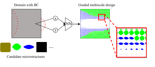
Fluid-flow devices with low dissipation, but high contact area, are of importance in many applications. A well-known strategy to design such devices is multi-scale topology optimization (MTO), where optimal microstructures are designed within each cell of a discretized domain. Unfortunately, MTO is computationally very expensive since one must perform homogenization of the evolving microstructures, during each step of the homogenization process. As an alternate, we propose here a graded multiscale topology optimization (GMTO) for designing fluid-flow devices. In the proposed method, several pre-selected but size-parameterized and orientable microstructures are used to fill the domain optimally. GMTO significantly reduces the computation while retaining many of the benefits of MTO.
In particular, GMTO is implemented here using a neural-network (NN) since: (1) homogenization can be performed off-line, and used by the NN during optimization, (2) it enables continuous switching between microstructures during optimization, (3) the number of design variables and computational effort is independent of number of microstructure used, and, (4) it supports automatic differentiation, thereby eliminating manual sensitivity analysis. Several numerical results are presented to illustrate the proposed framework.
Keywords Topology Optimization Stokes Flow Multiscale Neural Networks Fluid Microstructure
1 Introduction
Topology optimization is used extensively today in various disciplines [42]. When applied to fluid-flow problems, it addresses the following question [1]: "Where should fluid flow within a design domain?" As an example, consider the simple diffuser problem posed in fig. 2(a) where fluid enters on the left and exits on the right, as illustrated. The objective is to design the fluid flow path such that the dissipated power is minimized. In addition, a volume constraint is often imposed on the surrounding solid material (or equivalently, on the fluid space). Using topology optimization techniques described, for example in [9], one can solve this problem to arrive at the topology, i.e., fluid flow path, illustrated in fig. 2(b). For such simple problems, one can argue that topology optimization is not needed since the solution is often a single flow path [1].

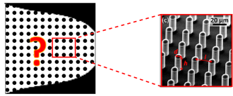
Topology optimization becomes more important when additional criteria come into play. For example, maximizing the fluid-solid contact area is critical in many applications including bio-sensors for detecting tumour cells [37], microfluidic devices for cell sorting [18, 25, 28, 34, 15], micro-channel heat sinks [57, 24, 36], and other microfluidic devices involving heat transfer and mass transportation/mixing mechanisms [6, 7]. In such applications, a heuristic strategy to increase the contact surface is to use micro-pillar arrays [26, 32] as illustrated in fig. 3.
While uniform cylindrical micro-pillars can increase the contact surface, they can also significantly increase the dissipated power loss [31, 8]. To balance the two, one can vary the the cylinder radii or, better still, use non-cylindrical micro-pillars, henceforth referred to as microstructures, with proper orientation for minimizing power loss and maximizing fluid-solid contact interface [53]. Optimizing the cross-section, size and orientation of the microstructures leads to a multi-scale fluid-flow topology optimization problem [53], the main focus of this paper.
In multi-scale topology optimization (MTO), optimal microstructures are designed in each cell of a discretized domain. Unfortunately, this can be very expensive [52] since one must carry out homogenization of the evolving microstructures [56] during each step of the global optimization process. Specifically, if is the number of elements (typically in the order of 1000s), is the number of global optimization steps (typically in the order of 100s), and is the cost of homogenization, then the MTO cost is at least . In this paper, we propose a graded MTO (GMTO) strategy that retains much of the advantages of MTO, but exhibits a significantly lower computational cost.
The remainder of this paper is organized as follows. In section 2 we review the literature on topology optimization for fluid flow problems, and summarize the main contributions of this paper. In section 3, we briefly review relevant technical background, followed by the proposed method in section 4. Numerical examples are illustrated in section 5, and conclusions are provided in section 6.
2 Related Work
In this section, we briefly review prior work on fluid-flow topology optimization methods. In particular, while many different strategies have been proposed [1, 10], we focus here on density-based methods.
2.1 Single-scale TO
Topology optimization for fluid-flow problems first appeared in 2003 in the seminal work of Borrvall and Petersson [9]. They presented the optimal layout of channel flows for minimal drag (or pressure drop), for Stokes equation with Brinkman–Darcy law equations under low Reynolds number (laminar flow conditions). Gersborg-Hansen et al. [19] continued this study and presented applications with low Reynolds numbers for microfluidic problems and micro-electro-mechanical devices. Guest and Prévost [22] solved the formulation of the Stokes–Darcy problem numerically using stabilized finite element methods. Wiker et al. [51] used the viscosity as a dependent parameter and presented examples of channels in a tree-shaped structure for a pure Darcy problem and mixed Stokes–Darcy flow. Pereira et al. [41] reproduced the classical examples presented by [9] for optimal channels designs considering Stokes–Darcy flow using polygonal meshes and provided an educational software written in MATLAB. Suárez et al.[44] applied topology optimization to non-Newtonian flows in arbitrary domains, using a virtual element method.
2.2 Multi-scale TO
Multiscale topology optimization (MTO) for fluid flow, as mentioned earlier, involves generating appropriate microstructures, i.e., generalization of micro-pillars, typically, in each finite element cell, for maximizing fluid permeability. Guest and Prévost [23] maximised the permeability of porous microstructures using a Darcy–Stokes interpolation [22] subject to isotropic symmetry constraints. This was extended in [21] to optimize microstructures for maximal stiffness and permeability. Bio-mimicking techniques have been demonstrated for achieving this goal [27] but are not proven to be optimal [53]. MTO that minimizes energy loss and offers high contact area was demonstrated in [53]. However, the volume fraction of the microstructures was pre-determined, and the surface contact area was not explicitly controlled.
2.3 Paper Contributions
In this work we extend a particular GMTO framework proposed in [12] for structural problems, to fluid flow problems. In structural GMTO, a total volume constraint is imposed, whereas here, a total contact area constraint is more critical, changing the type of microstructures one must choose. Further, microstructure orientation is not typically considered in structural problems (due to potential loss in connectivity), but it plays an important role in fluid problems.
The proposed GMTO strategy is based on a neural-network based optimization framework for the the following reasons: (1) it implicitly guarantees the partition of unity, i.e., ensures that the net volume fraction of microstructures in each cell is unity, as described later on, (2) it supports automatic differentiation, and (3) the number of design variables is only weakly dependent on the number of pre-selected microstructures.
3 Technical Background
3.1 Fluid Flow Governing Equations
We assume here a low-Reynolds in-compressible Stokes flow, i.e.,
| (1a) | |||
| (1b) | |||
| (1c) | |||
where and p are the velocity and pressure of the fluid, is its viscosity, denotes the rate-of-strain tensor, is the inverse permeability tensor; the fluid is assumed to be of unit density.
3.2 Problem Formulation
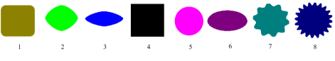
We also assume that a set of microstuctures have been pre-selected. Specifically, we consider the microstructures illustrated in fig. 4 (selected from various sources [23, 22, 3, 35, 53, 4]) that exhibit a wide range of permeability and contact area. Each of these microstructures can be scaled and oriented for optimal flow. For future reference, they are named as follows: 1: Squircle, 2: Fish-body-1, 3: Fish-body-2, 4: Square, 5: Circle, 6: Ellipse, 7: Mucosa-10, and 8: Mucosa-20. Such microstructures are often seen in nature; for example, mucosa-like structures are known to be present in the human intestine [4].
A typical design domain with prescribed flow boundary conditions is illustrated in fig. 5. We seek to compute an optimal multiscale design where we determine, in each finite element cell, the appropriate microstructure, its size (gradation) and orientation. The objective is to minimize the dissipated power subject to a total contact area (i.e., perimeter in 2D) constraint. The strategy we adopt is to pre-compute the permeability and contact area of each of the microstructures as a function of its size and orientation, and exploit these for a global multi-scale fluid-flow optimization.
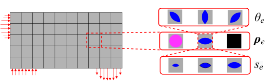
Towards this end, we introduce the following design variables. The presence or absence of a microstructure at any element will be captured by the set of density variables ; see fig. 5. Ideally should take a binary value subject to partition of unity constraint . However, for gradient-based optimization, we will let and drive it towards through penalization (once again subject to the partition of unity constraint).
We control the size of all the microstructures at any element by the scalar design variable (see fig. 5), where 0 denotes completely filled with fluid, and 1 denotes maximum size of the microstructure(s). Note that: (1) a single variable controls the size of all microstructures at that point, (2) means that the microstructures at that element are at their maximum size (that can fit into that cell); however, it does not imply that the cell is fully solid, and (3) as we drive towards only one microstructure of that size will prevail at that element.
Finally, the orientation of all the microstructures at , with respect to the axis, will be denoted by (see fig. 5). Thus the design variables associated with each element will be denoted by .
3.3 Effective Permeability through Numerical Homogenization
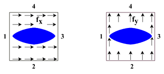
Prior to carrying out global optimization, we pre-compute the permeability tensor of each microstructure at discrete sizes. The components of can be computed by posing two low-Reynolds in-compressible Stokes flow problems over a unit cell, with unit body forces and , respectively, as illustrated in fig. 6. The boundary conditions for both problems are as follows: (a) boundaries 1 and 3 are coupled through periodic boundary conditions for velocity and pressure, and (b) boundaries 2 and 4 are similarly coupled. The velocities obtained by solving the problem in fig. 6a are denoted by and , while those obtained from fig. 6b are denoted by and . The components of the permeability tensor are then defined as [2, 30, 45]:
| (2) |
where is the volume of the unit cell. Observe that, at a default orientation, all the microstructures in fig. 4 are symmetric about the two axis. Therefore, the off-diagonals are zero, i.e., .
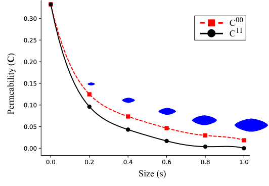
We compute the two remaining components for each microstructure at a finite number of sizes, at default orientation, using the implementation provided in [2]. Then, two interpolating and positive polynomials [29] and are constructed from these samples. As an example, the polynomials for a fish-body-type microstructure are illustrated in fig. 7. In this paper, we use a degree polynomial.
The orientation is then accounted for via the following tensor operation [30]:
| (3) |
Finally, since multiple microstructure can co-exist at any element, the following penalization scheme is proposed to ensure that we drive towards (subscript has been suppressed for simplicity):
| (4) |
where the penalization discourages microstructure mixing.
Observe that the pre-computation cost is approximately , where is the number of size samples (6 in this paper) , is the number of microstructures (8 in this paper) and is the cost of homogenization. This is significantly lower than the cost for MTO.
3.4 Contact area
Observe that the contact area of a microstructure is proportional to its size , and independent of orientation . Thus, it is sufficient to compute the maximum contact area at for each microstructure. The contact areas are then combined as follows (subscript has been suppressed for simplicity):
| (5) |
3.5 Volume Constraint
One can also impose a constraint on the total fluid volume allowed; this constraint is mainly used in validation experiments (please see section 5.1.1). Similar to the contact area computation, the total volume occupied by the fluid is given by:
| (6) |
where is the fraction of the volume occupied by a microstructure at maximum size.
3.6 Fluid Flow Finite Element Analysis
For the global fluid flow analysis, we use quadrilateral Q2-Q1 (Taylor-Hood) elements. The elemental stiffness matrix and degrees of freedom vector for the governing equation (see section 3.1) are given by (see [41] for details):
| (7) |
where
| (8a) | |||
| (8b) | |||
| (8c) | |||
| (8d) | |||
| (8e) | |||
where and are the velocity and pressure basis functions, and represent elemental velocity and pressure degrees of freedom respectively and is the element permeability matrix (described previously). In order to uniquely define the pressure field, a zero mean condition is enforced.
3.7 Optimization Problem
Consequently, one can pose the GMTO problem in a finite-element setting as:
| (9a) | |||||
| subject to | (9b) | ||||
| (9c) | |||||
| (9d) | |||||
| (9e) | |||||
| (9f) | |||||
| (9g) | |||||
| (9h) | |||||
where is the dissipated power, is the lower bound on the total contact area, is the upper bound on the total volume fraction, is the total unit cell volume, and , and are the global stiffness, degrees of freedom and the boundary conditions respectively. In the optimization problem, either we impose volume constraint, eq. 9d, for validation (please see section 5.1.1) or contact area constraint, eq. 9c, for other numerical experiments.
In the above direct formulation, the number of design variables is proportional to the mesh size. Further, the partition of unity, and bound constraints must be strictly enforced over each element. In this paper, we avoid these issues by indirectly controlling the design variables via a coordinate-based neural-network [14, 13] described next.
4 Proposed Method
4.1 Neural Network
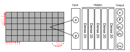
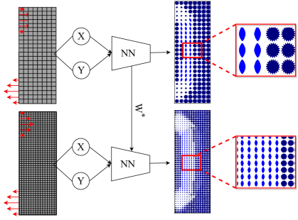
The proposed neural-network (NN) architecture is illustrated in fig. 8, and it consists of the following entities:
-
1.
Input Layer: The input to the NN are points within the domain. Although these points can be arbitrary, they correspond here to the center of the elements.
-
2.
Hidden Layers: The hidden layers consist of a series of dense fully connected LeakyReLU activated neurons.
-
3.
Output Layer: The output layer consists of neurons correspond to the design variables for each element . Further, the neurons associated with the density variables are controlled by a softmax function such that the partition of unity and physical validity are automatically satisfied. The output neuron associated with the size parameter is controlled via a Sigmoid function , ensuring that . Finally, the output neuron associated with the orientation parameter is also controlled via a Sigmoid function and scaled as . Thus, no additional box constraints are needed.
-
4.
NN Design Variables: The weights and bias associated with the NN, denoted by the , now become the primary design variables, i.e., we have and .
Thus the strategy is to perform GMTO via the NN weights , i.e., eq. 9 reduces to:
| (10a) | |||||
| subject to | (10b) | ||||
| (10c) | |||||
| (10d) | |||||
Observe that: (1) no additional constraint is needed since they are automatically satisfied, and (2) the number of design variables () is independent of the mesh size and the number of microstructures.
4.2 Loss Function
We now consider solving the NN-based optimization problem in eq. 10. Since neural networks are designed to minimize an unconstrained loss function, we convert the constrained minimization problem into a loss function minimization by employing the augmented Lagrangian scheme [5]. Specifically, the loss function is defined as
| (11) |
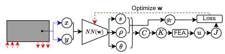
where the parameters and are updated during each iteration, making the enforcement of the constraint stricter as the optimization progresses (see discussion below). Thus the overall framework is illustrated in fig. 9.
4.3 Sensitivity Analysis
For minimizing the loss function in eq. 11 we use L-BFGS [33], a well-known optimization technique. Since L-BFGS is a gradient-based optimizer, it requires sensitivities, i.e., derivative of the loss function in eq. 11 with respect to the design variables . Fortunately, one can exploit modern automatic differentiation frameworks [11] to avoid manual sensitivity calculations. In particular, we use PyTorch [40] as an implementation environment, resulting in an end-to-end differentiable framework.
4.4 Algorithm
The algorithm for the proposed framework is summarized below. First, we generate the dataset consisting of permeability matrices (at various sizes) and contact area values for the pre-selected microstructures (line 2). Polynomials are constructed to fit the data (line 3).
Next the domain is discretized for finite element analysis, and the stiffness matrix components are computed (lines 4-5). The mesh is sampled at the center of each element (line 6); these serve as inputs to the NN. The augmented Lagrangian parameters , , the penalty parameter and NN weights are initialized (line 7).
In the main iteration, the design variables are computed using the NN (line 9), followed by the computation of the permeability matrices for each element (line 10). These are then used to construct the stiffness matrix and to solve for the velocity and pressure (line 11 - line 12). Then the objective and contact area constraint are computed (lines 13 - 14), leading to the loss function (line 15). The sensitivities are computed in an automated fashion (line 16). The weights are then updated using L-BFGS optimization scheme (line 17). Finally the augmented Lagrangian multipliers and penalty parameters are updated (line 18 - 20). The process is repeated until termination, i.e., until the relative change in loss is below a certain threshold or the iterations exceed a maximum value.
5 Numerical Experiments
In this section, we conduct several experiments to illustrate the method and algorithm. All experiments are conducted on a MacBook Air M2, using the PyTorch [40] environment. The default settings are as follows:
-
•
Neural Network: The NN comprises of 2 LeakyReLU-activated hidden layers with 20 neurons in each layer. This corresponds approximately to 4730 design variables. The initial values for are determined via Xavier weight initialization [20], with a seed value of 77.
-
•
Candidate microstructures: A set of 8 predefined microstructures (fig. 4) is used in the experiments. Numerical homogenization is performed at six uniformly spaced sample points. A quintic polynomial is then used to interpolate the components of the sampled permeabiliity matrix.
-
•
Material Penalization: The penalization is incremented every iteration by 0.02 using the continuation scheme [43], starting from a value of 1, with a maximum value of 8.
-
•
Loss Function: The initial constraint penalty is = 0.05, and is increased by per epoch.
-
•
Optimizer: L-BFGS optimizer with a strong Wolfe line search function is used [39]. The maximum number of iterations (epochs) is set to 25. For convergence of optimization, we set change in loss .
For reference, the offline numerical homogenization of the 8 microstructures, at 6 different sizes, was performed in 16 seconds.
5.1 Double-pipe Problem
5.1.1 Validation
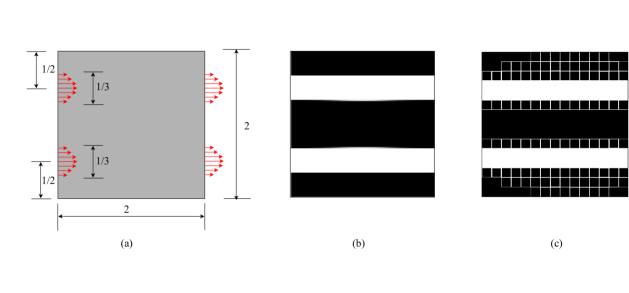
In the first experiment, we validate the proposed method using the double-pipe problem considered in [9], and illustrated in fig. 10(a). The objective is to find the optimal topology of fluid volume fraction that minimizes the dissipated power; contact area constraint is not imposed. The domain is discretized into 15x15 elements. The authors of [9] report the topology illustrated in fig. 10(b), with an objective value of . In the proposed method, we use a single square microstructure (see fig. 4), and arrive at the topology illustrated in fig. 10(c), with an objective of . We observe partial infills in some of the cells since the size is not penalized towards , i.e., we allow for intermediate sizes.
5.1.2 Impact of microstructures
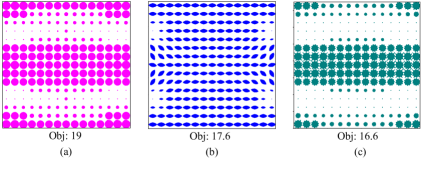
Next we replace the square microstructure with three other microstructures, namely the circle, fish-body-2, and Mucosa-10 (see fig. 4), one at a time, and study the impact of the microstructure on the dissipated power; the desired contact area is kept constant at . However, no constraint is imposed on the volume fraction.
The resulting topologies are illustrated in fig. 11. Note that for the same contact area, the permeability of the fish-body-2 is higher than that of circle. This results in the fish-body-2 having a smaller dissipated power compared to the circle. On the other hand, despite a lower-permeability, Mucosa-10 performs better than the fish-body-2 since its contact area is significantly higher.
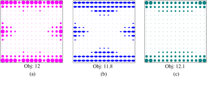
We then reduced the surface constraint to ; the results are illustrated in fig. 12. Now, fish-body-2 and circle perform better than Mucosa-10. This experiment illustrates that the choice of a microstructure critically depends on the constraints imposed.
5.2 Diffuser Problem
5.2.1 Validation
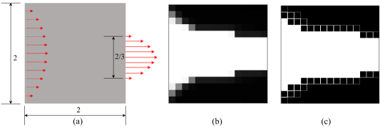
For the second set of experiments, we consider the diffuser problem discussed in [9], and illustrated in fig. 13(a). In the first experiment, the objective is to find the optimal topology of fluid volume fraction that minimizes the dissipated power; contact area constraint is not imposed. The domain is discretized into 15x15 elements. The authors of [9] report the topology illustrated in fig. 13(b), with an objective value of . Next, in the proposed method, the square microstructure is once again used for optimization. The final topology is illustrated in fig. 13(c), consistent with fig. 13(b), with an objective of [9]. The single scale optimization was performed in five seconds.
5.2.2 Multiple microstructures
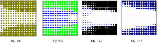
Two central hypotheses of the current work is that one can achieve better designs with larger number of candidate microstructures, and that the framework is computationally insensitive to the number of candidates. To validate, we consider again the problem in fig. 13(a), but instead of the volume constraint, we impose a contact area constraint of . We consider the first microstructures, where , and study the impact on the dissipated power and computational time. The resulting topologies are illustrated in fig. 14, as expected, the objective improves as we allow for larger number of microstructures. The computational time was approximately 62 seconds, independent of the number of microstructures.
5.3 Bent Pipe Problem
5.3.1 Validation
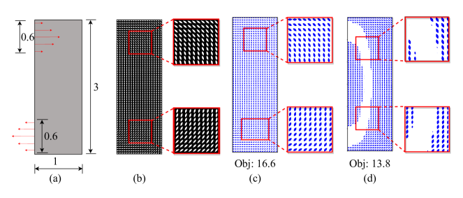
Next, we consider the bent-pipe problem proposed in [53], and illustrated in fig. 15(a). The domain is discretized into 20x60 elements. In [53], a two-scale topology optimization was carried out to minimize the dissipated power, with a constraint that the optimal microstructure must occupy exactly 25 percent of each unit cell. The reported topology is illustrated in fig. 15(b); the final dissipated power was not reported. However, as noted in [53], the computed microstructures resemble the fish-body.
In the proposed method, the fish-body-2 microstructure was chosen a priori, and its size was fixed to occupy 25 percent of each unit cell, as in [53]. The orientation of each microstructure was optimized, resulting in the design illustrated in fig. 15(c) with the final dissipated power of 16.6. Not surprisingly, the final topology is similar to fig. 15(b).
To improve on this design, we removed the constraint of the 25 percent unit-cell volume occupation, and instead imposed a total (global) volume constraint of 25 percent, i.e., we allowed the size of each microstructure to vary as well. The resulting topology is illustrated in fig. 15(d). As one can observe, the dissipated power further reduces to 13.8.
5.3.2 Fluid flow validation
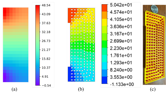
Next, for the above problem, we compute the pressure predicted using the GMTO framework and compare it against full-scale fluid flow simulation using Ansys. Due to challenges in importing the geometry into ANSYS, the domain was discretized using a coarser mesh of 8x24 elements.
The pressure prediction using the homogenization-based GMTO framework is illustrated in fig. 16(a); the total pressure drop is approximately 49.0 Pascals. We then exported the optimized topology as an ".stl" file and imported it into ANSYS [16] for full-scale fluid-flow simulation. The pressure drop predicted using ANSYS is illustrated in fig. 16(b); the total pressure drop is approximately 51.17 Pascals. The 3d printed part is illustrated in fig. 16(c).
5.3.3 Pareto Designs
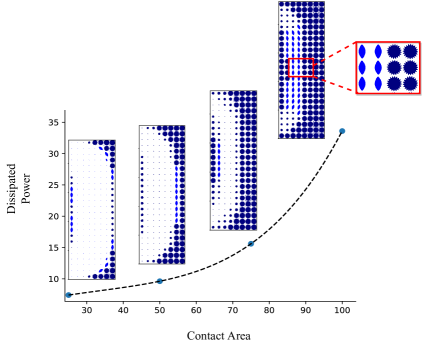
Exploring the Pareto-front is critical in making design choices and understanding the trade-off between the objective (dissipated power) and constraint (contact area). To illustrate this, we computed the optimal topologies for various values of contact areas for the bent-pipe problem, by considering all 8 microstructures; the results are illustrated in fig. 17. Observe that as expected, the dissipated power increases with the contact area. Further, one can observe that regions with high fluid flow (see inset) are dominated by fish-body-2 (that exhibits high permeability), whereas regions with low fluid flow are dominated by Mucosa-20 (that exhibits high contact area).
5.3.4 Resampling
A subtle but important aspect of the proposed framework is that since the design fields (density, orientation, and size) are represented globally using the neural-network, one can obtain high-resolution topologies with no additional cost. To illustrate, suppose we have computed the optimal weights and optimal topology for a given mesh discretization. We can then sample the domain at a higher resolution using the optimized weights , resulting in a more-detailed topology (Note that this is not a simple linear interpolation.) This is illustrated in fig. 18 where we optimize using a 8 × 24 mesh, and then re-sample using a 16 × 48 mesh.
6 Conclusion
A graded multi-scale fluid flow topology optimization framework was proposed where homogenization is performed off-line, followed by global optimization. Two-scale designs with high contact area and low dissipated power were generated through the framework. Furthermore, the computational cost was found to be independent of the number of pre-selected microstructures. The neural-network configuration ensured that the partition of unity constraint was automatically satisfied. Finally, the PyTorch environment allowed for automated sensitivity computation.
Currently, the framework is limited to microstructures with a single-size parameter. A contact area constraint, whose value was arbitrarily chosen, was imposed in the current work. We plan to explore extensions to multi-physics problems such as convection-driven heat transfer problems [17] where the contact area constraint is determined through the underlying physics. Furthermore, it will be interesting to combine the proposed framework with data-driven methods [47].
Compliance with ethical standards
The authors declare that they have no conflict of interest.
Replication of Results
The Python code pertinent to this paper is available at github.com/UW-ERSL/FluTO.
Acknowledgement
The authors would like to thank the support of National Science Foundation through grant CMMI 1561899. The authors acknowledge Subodh Subedi for helping with the 3D printing.
References
- [1] Joe Alexandersen and Casper Schousboe Andreasen. A review of topology optimisation for fluid-based problems. Fluids, 5(1):29, 2020.
- [2] Erik Andreassen and Casper Schousboe Andreasen. How to determine composite material properties using numerical homogenization. Computational Materials Science, 83:488–495, 2014.
- [3] El-Sayed Aziz, Constantin Chassapis, Sven Esche, Sumei Dai, Shanjun Xu, and Ruiqing Jia. Online wind tunnel laboratory. In 2008 Annual Conference & Exposition, pages 13–949, 2008.
- [4] Valentina Balbi and Pasquale Ciarletta. Morpho-elasticity of intestinal villi. Journal of the Royal Society Interface, 10(82):20130109, 2013.
- [5] Dimitri P Bertsekas. Constrained optimization and Lagrange multiplier methods. Academic press, 2014.
- [6] Gregory D Bixler and Bharat Bhushan. Bioinspired rice leaf and butterfly wing surface structures combining shark skin and lotus effects. Soft matter, 8(44):11271–11284, 2012.
- [7] Gregory D Bixler and Bharat Bhushan. Fluid drag reduction and efficient self-cleaning with rice leaf and butterfly wing bioinspired surfaces. Nanoscale, 5(17):7685–7710, 2013.
- [8] Humberto Bocanegra Evans, Serdar Gorumlu, Burak Aksak, Luciano Castillo, and Jian Sheng. Holographic microscopy and microfluidics platform for measuring wall stress and 3d flow over surfaces textured by micro-pillars. Scientific reports, 6(1):1–12, 2016.
- [9] Thomas Borrvall and Joakim Petersson. Topology optimization of fluids in stokes flow. International journal for numerical methods in fluids, 41(1):77–107, 2003.
- [10] Vivien J Challis and James K Guest. Level set topology optimization of fluids in stokes flow. International journal for numerical methods in engineering, 79(10):1284–1308, 2009.
- [11] Aaditya Chandrasekhar, Saketh Sridhara, and Krishnan Suresh. Auto: a framework for automatic differentiation in topology optimization. Structural and Multidisciplinary Optimization, 64(6):4355–4365, 2021.
- [12] Aaditya Chandrasekhar, Saketh Sridhara, and Krishnan Suresh. Gm-tounn: Graded multiscale topology optimization using neural networks. arXiv preprint arXiv:2204.06682, 2022.
- [13] Aaditya Chandrasekhar and Krishnan Suresh. Multi-material topology optimization using neural networks. Computer-Aided Design, 136:103017, 2021.
- [14] Aaditya Chandrasekhar and Krishnan Suresh. Tounn: topology optimization using neural networks. Structural and Multidisciplinary Optimization, 63(3):1135–1149, 2021.
- [15] Jin-Woo Choi, Kwang W Oh, Jennifer H Thomas, William R Heineman, H Brian Halsall, Joseph H Nevin, Arthur J Helmicki, H Thurman Henderson, and Chong H Ahn. An integrated microfluidic biochemical detection system for protein analysis with magnetic bead-based sampling capabilities. Lab on a Chip, 2(1):27–30, 2002.
- [16] Gabriel J DeSalvo and John A Swanson. ANSYS Engineering Analysis System: User’s Manual. Swanson Analysis Systems, 1979.
- [17] Sumer B Dilgen, Cetin B Dilgen, David R Fuhrman, Ole Sigmund, and Boyan S Lazarov. Density based topology optimization of turbulent flow heat transfer systems. Structural and Multidisciplinary Optimization, 57(5):1905–1918, 2018.
- [18] Z Hugh Fan, Shakuntala Mangru, Russ Granzow, Paul Heaney, Wen Ho, Qianping Dong, and Rajan Kumar. Dynamic dna hybridization on a chip using paramagnetic beads. Analytical chemistry, 71(21):4851–4859, 1999.
- [19] Allan Gersborg-Hansen, Ole Sigmund, and Robert B Haber. Topology optimization of channel flow problems. Structural and multidisciplinary optimization, 30(3):181–192, 2005.
- [20] Xavier Glorot and Yoshua Bengio. Understanding the difficulty of training deep feedforward neural networks. In Proceedings of the thirteenth international conference on artificial intelligence and statistics, pages 249–256. JMLR Workshop and Conference Proceedings, 2010.
- [21] James K Guest and Jean H Prévost. Optimizing multifunctional materials: design of microstructures for maximized stiffness and fluid permeability. International Journal of Solids and Structures, 43(22-23):7028–7047, 2006.
- [22] James K Guest and Jean H Prévost. Topology optimization of creeping fluid flows using a darcy–stokes finite element. International Journal for Numerical Methods in Engineering, 66(3):461–484, 2006.
- [23] James K Guest and Jean H Prévost. Design of maximum permeability material structures. Computer Methods in Applied Mechanics and Engineering, 196(4-6):1006–1017, 2007.
- [24] Dongzhi Guo, Alan JH McGaughey, Jinsheng Gao, Gary K Fedder, Minyoung Lee, and Shi-Chune Yao. Multiphysics modeling of a micro-scale stirling refrigeration system. International journal of thermal sciences, 74:44–52, 2013.
- [25] Mark A Hayes, Nolan A Polson, Allison N Phayre, and Antonio A Garcia. Flow-based microimmunoassay. Analytical chemistry, 73(24):5896–5902, 2001.
- [26] Xiaowen Huang, Jianchun Wang, Tenghao Li, Jianmei Wang, Min Xu, Weixing Yu, Abdel El Abed, and Xuming Zhang. Review on optofluidic microreactors for artificial photosynthesis. Beilstein journal of nanotechnology, 9(1):30–41, 2018.
- [27] Zoran Jakšić and Olga Jakšić. Biomimetic nanomembranes: An overview. Biomimetics, 5(2):24, 2020.
- [28] Guifeng Jiang and D Jed Harrison. mrna isolation in a microfluidic device for eventual integration of cdna library construction. Analyst, 125(12):2176–2179, 2000.
- [29] Tej Kumar, Saketh Sridhara, Bhagyashree Prabhune, and Krishnan Suresh. Spectral decomposition for graded multi-scale topology optimization. Computer Methods in Applied Mechanics and Engineering, 377:113670, 2021.
- [30] PS Lang, A Paluszny, and RW Zimmerman. Permeability tensor of three-dimensional fractured porous rock and a comparison to trace map predictions. Journal of Geophysical Research: Solid Earth, 119(8):6288–6307, 2014.
- [31] George V Lauder, Dylan K Wainwright, August G Domel, James C Weaver, Li Wen, and Katia Bertoldi. Structure, biomimetics, and fluid dynamics of fish skin surfaces. Physical Review Fluids, 1(6):060502, 2016.
- [32] Lin Li, Rong Chen, Qiang Liao, Xun Zhu, Guanyi Wang, and Dongye Wang. High surface area optofluidic microreactor for redox mediated photocatalytic water splitting. International journal of hydrogen energy, 39(33):19270–19276, 2014.
- [33] DC Liu and J Nocedal. On the limited memory method for large scale optimization: Mathematical programming b. 1989.
- [34] Yan-Jun Liu, Shi-Shang Guo, Zhi-Ling Zhang, Wei-Hua Huang, Damien Baigl, Min Xie, Yong Chen, and Dai-Wen Pang. A micropillar-integrated smart microfluidic device for specific capture and sorting of cells. Electrophoresis, 28(24):4713–4722, 2007.
- [35] Mohammed G Mohammed, Arianne F Messerman, Bryan D Mayhan, and Kathleen M Trauth. Theory and practice of the hydrodynamic redesign of artificial hellbender habitat. Herpetological Review, 47(4):586–591, 2016.
- [36] Matthew Moran, Danielle Wesolek, Bruk Berhane, and Keith Rebello. Microsystem cooler development. In 2nd International Energy Conversion Engineering Conference, page 5611, 2004.
- [37] Sunitha Nagrath, Lecia V Sequist, Shyamala Maheswaran, Daphne W Bell, Daniel Irimia, Lindsey Ulkus, Matthew R Smith, Eunice L Kwak, Subba Digumarthy, Alona Muzikansky, et al. Isolation of rare circulating tumour cells in cancer patients by microchip technology. Nature, 450(7173):1235–1239, 2007.
- [38] Cong Hong Phong Nguyen and Young Choi. Multiscale design of functionally graded cellular structures for additive manufacturing using level-set descriptions. Structural and Multidisciplinary Optimization, 64(4):1983–1995, 2021.
- [39] Jorge Nocedal and Stephen J Wright. Numerical optimization. Springer, 1999.
- [40] Adam Paszke, Sam Gross, Francisco Massa, Adam Lerer, James Bradbury, Gregory Chanan, Trevor Killeen, Zeming Lin, Natalia Gimelshein, Luca Antiga, Alban Desmaison, Andreas Kopf, Edward Yang, Zachary DeVito, Martin Raison, Alykhan Tejani, Sasank Chilamkurthy, Benoit Steiner, Lu Fang, Junjie Bai, and Soumith Chintala. Pytorch: An imperative style, high-performance deep learning library. In H. Wallach, H. Larochelle, A. Beygelzimer, F. d'Alché-Buc, E. Fox, and R. Garnett, editors, Advances in Neural Information Processing Systems 32, pages 8024–8035. Curran Associates, Inc., 2019.
- [41] Anderson Pereira, Cameron Talischi, Glaucio H Paulino, Ivan F M Menezes, and Marcio S Carvalho. Fluid flow topology optimization in polytop: stability and computational implementation. Structural and Multidisciplinary Optimization, 54(5):1345–1364, 2016.
- [42] O. Sigmund and K. Maute. Topology optimization approaches: A comparative review. Structural and Multidisciplinary Optimization, 48(6):1031–1055, 2013.
- [43] Ole Sigmund and Joakim Petersson. Numerical instabilities in topology optimization: a survey on procedures dealing with checkerboards, mesh-dependencies and local minima. Structural optimization, 16(1):68–75, 1998.
- [44] Miguel AA Suárez, Juan S Romero, Anderson Pereira, and Ivan FM Menezes. On the virtual element method for topology optimization of non-newtonian fluid-flow problems. Engineering with Computers, pages 1–22, 2022.
- [45] Rafael S Vianna, Alexsander M Cunha, Rodrigo BV Azeredo, Ricardo Leiderman, and Andre Pereira. Computing effective permeability of porous media with fem and micro-ct: An educational approach. Fluids, 5(1):16, 2020.
- [46] Liwei Wang, Siyu Tao, Ping Zhu, and Wei Chen. Data-driven topology optimization with multiclass microstructures using latent variable gaussian process. Journal of Mechanical Design, 143(3), 2021.
- [47] Liwei Wang, Anton van Beek, Daicong Da, Yu-Chin Chan, Ping Zhu, and Wei Chen. Data-driven multiscale design of cellular composites with multiclass microstructures for natural frequency maximization. Composite Structures, 280:114949, 2022.
- [48] Yingjun Wang, Hang Xu, and Damiano Pasini. Multiscale isogeometric topology optimization for lattice materials. Computer Methods in Applied Mechanics and Engineering, 316:568–585, 2017.
- [49] Seth Watts, William Arrighi, Jun Kudo, Daniel A Tortorelli, and Daniel A White. Simple, accurate surrogate models of the elastic response of three-dimensional open truss micro-architectures with applications to multiscale topology design. Structural and Multidisciplinary Optimization, 60(5):1887–1920, 2019.
- [50] Daniel A White, William J Arrighi, Jun Kudo, and Seth E Watts. Multiscale topology optimization using neural network surrogate models. Computer Methods in Applied Mechanics and Engineering, 346:1118–1135, 2019.
- [51] Niclas Wiker, Anders Klarbring, and Thomas Borrvall. Topology optimization of regions of darcy and stokes flow. International journal for numerical methods in engineering, 69(7):1374–1404, 2007.
- [52] Jun Wu, Ole Sigmund, and Jeroen P Groen. Topology optimization of multi-scale structures: a review. Structural and Multidisciplinary Optimization, 63(3):1455–1480, 2021.
- [53] Tong Wu. Topology Optimization of Multiscale Structures Coupling Fluid, Thermal and Mechanical Analysis. PhD thesis, Purdue University Graduate School, 2019.
- [54] Ruijie Zhao, Junpeng Zhao, and Chunjie Wang. Stress-constrained multiscale topology optimization with connectable graded microstructures using the worst-case analysis. International Journal for Numerical Methods in Engineering, 123(8):1882–1906, 2022.
- [55] Li Zheng, Siddhant Kumar, and Dennis M Kochmann. Data-driven topology optimization of spinodoid metamaterials with seamlessly tunable anisotropy. Computer Methods in Applied Mechanics and Engineering, 383:113894, 2021.
- [56] Shiwei Zhou and Qing Li. Design of graded two-phase microstructures for tailored elasticity gradients. Journal of Materials Science, 43(15):5157–5167, 2008.
- [57] Yangying Zhu, Dion S Antao, Zhengmao Lu, Sivanand Somasundaram, Tiejun Zhang, and Evelyn N Wang. Prediction and characterization of dry-out heat flux in micropillar wick structures. Langmuir, 32(7):1920–1927, 2016.