Quantum Vision Transformers

Abstract

We design and analyse quantum transformers, extending the state-of- the-art classical transformer neural network architectures known to be very performant in natural language processing and image analysis. Building upon the previous work of using parametrised quantum circuits for data loading and orthogonal neural layers, we introduce three types of quantum attention mechanisms, including a quantum transformer based on compound matrices. These quantum architectures can be built using shallow quantum circuits and can provide qualitatively different classification models. We performed extensive simulations of the quantum transformers on standard medical image datasets that showed competitive, and at times better, performance compared with the best classical transformers and other classical benchmarks. Computational complexity of our quantum attention layer proves to be advantageous compared with the classical algorithm, with respect to the size of the classified images. Our quantum architectures have thousands of parameters, compared with the best classical methods with millions of parameters. Finally, we have implemented our quantum transformers on superconducting quantum computers and obtained encouraging results for up to six qubit experiments.

I Introduction

Quantum machine learning BWP⁺ (17) uses quantum computation in order to provide novel and powerful tools that can be used to enhance the performance of classical machine learning algorithms. One way to do this is to use efficient quantum methods for linear algebra both in more traditional learning algorithms, including similarity-based classification JDM⁺ (21); LMR (13), linear systems solvers HHL (09), dimensionality reduction techniques LMR (14), clustering algorithms KLLP (19); AdW (20); KL (21), recommendation systems KP (17); WGLZ (21), as well as in deep learning KLP (19). An alternative is to use parametrised quantum circuits as quantum neural networks that could potentially be more powerful by exploring a higher-dimensional optimization space CCL (19); BCLK⁺ (21); CAB⁺ (20) or by providing interesting properties, like orthogonality or unitarity KLM (21); KBLL (22).

In this work, we focus on transformers, a recent neural network architecture VSP⁺ (17) that has been proposed both for Natural Language Processing DCLT (18) and for visual tasks DBK⁺ (20), and has provided state-of-the-art performance across different tasks and datasets TDBM (20).

At a high level, transformers are neural networks that use an attention mechanism that takes into account the global context while processing the entire input data element-wise. In the case of visual analysis, for example, images are divided into smaller patches, and instead of simply performing patch-wise operations with fixed size kernels, a transformer learns attention coefficients per patch that weigh the attention paid to the rest of the image by each patch. In the case of visual recognition or text understanding, the context of each element is vital, and the transformer can capture more global correlations between parts of the sentence or the image than convolutional neural networks without an attention mechanism DBK⁺ (20).

Fig.1 shows a high-level representation of a Vision Transformer architecture, in line with DBK⁺ (20). The first part consists of dividing the images into patches, reformatted as vectors. Then, a number of transformer layers are applied, one of which is described in Fig.3. Last, the classification at the end happens through a fully connected layer. A key ingredient inside the transformer layer is the attention mechanism (Fig.4), which is trained to weigh each image patch in its global context. While extracting information from each patch, the network simultaneously learns how much attention a patch should pay to the other patchess. More details on classical transformers are given in Section II.

In one related work, classical transformer architectures and attention mechanisms have been used to perform quantum tomography CGW⁺ (21). Moreover, a quantum-enhanced transformer for sentiment analysis has been proposed in DSHC⁺ (22), and a self-attention mechanism for text classification has been used in LZW (22). All these results use standard variational quantum circuits for the neural networks, and the attention coefficients are calculated classically. A method for using a natively quantum attention mechanism for reinforcement learning has also been proposed in SWIK (22). YS (22) performed semiconductor defect detection using quantum self-attention, also using standard variational quantum circuits. We also note the proposal of CCL (19) for variational circuits with similarities to convolutional neural networks for general purpose image classification.

Our approach differs from the above-mentioned approaches in three key aspects. Firstly, we focus on quantum vision transformers and image classification tasks. In addition to a quantum translation of the classical vision transformer, a novel and natively quantum method is proposed in this work. This method provides what we call a compound transformer, which invokes Clifford Algebra operations that would be harder to compute classically. Finally, the different parametrised quantum circuits proposed in our work are supported by linear algebraic tools to calculate gradients and other properties, making them much more Noisy Intermediate-Scale Quantum (NISQ)-friendly with proven scalability, in contrast to variational QC approaches which lack proof of scalability MNKF (18). This advantage in scalability of our proposed parametrised quantum circuits is made possible by the use of a specific amplitude encoding for translating vectors as quantum states, and consistent use of hamming-weight preserving quantum gates instead of general quantum ansatz CAB⁺ (20). While we focus on vision transformers and benchmark our methods on vision tasks, our work could open the way for other applications, for example on textual data where transformers have been proven to be particularly efficient DCLT (18).

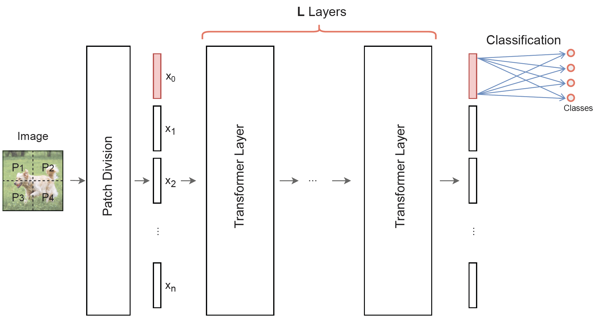
Figure 1: Representation of a Vision Transformer network architecture. DBK⁺ (20).

Our Results

We provide now a more detailed description of our results. We propose two types of quantum transformers, and apply the novel architectures to visual tasks. The main ingredient in a transformer is the attention mechanism, shown in Fig.4. We focus on leveraging QC on this part of the architecture. Other parts of the transformer architecture shown in Fig.1 and Fig.3 are derived from two previous works JDM⁺ (21); KLM (21).

In the first approach, coined the Orthogonal Transformer, we designed a quantum analogue for each of the two main components of a classical attention mechanism. The classical attention mechanism (Fig.4) starts with fully connected linear layers, where each input, or patch, $x_{i}$ is a vector that corresponds to a part of the image and is multiplied by a weight matrix $V$. To perform this operation quantumly, we use an orthogonal quantum layer, where a parametrised quantum circuit consisting of Reconfigurable Beam Splitter ($RBS$) gates is applied to a unary amplitude encoding of the input (see Sections III.1 and III.2 for details). An example of such an orthogonal layer has been defined in KLM (21), and these results are extended in this work by definition of new architectures for these layers, including ones with only logarithmic depth.

The second step of the attention mechanism is the interaction between patches. We define parametrised quantum circuits to learn the attention coefficients $A_{ij}$ by performing the linear-algebraic operation $x_{i}^{T}Wx_{j}$ for a trainable orthogonal matrix $W$ and all pairs of patches $x_{i}$ and $x_{j}$. After that, a simple non linearity is applied to obtain each output $y_{i}$.

The two steps of the attention mechanism described above can be applied with separate quantum circuits. In addition, a global quantum attention mechanism is also defined for forward inference after the matrices $V$ and $W$ have been trained. For this, a quantum data loader for matrices is used, where for each patch of the input, the entire matrix whose rows are the patches re-scaled by the attention weights are loaded. Once all patches are loaded in this attention-weighted superposition, the quantum circuit that applies $V$ on a patch is applied to provide a quantum version of an attention mechanism from which the classical output of the layer can be extracted (see also Section IV.3).

In Section IV.4, a second approach is described that is a more natively quantum version of a transformer. This architecture is termed a Compound Transformer, since it uses quantum layers that perform a linear algebraic operation that multiplies the input with a trainable second-order compound matrix. The main idea is that all patches are loaded in superposition, and then a trainable orthogonal matrix is applied that gives different attention to each patch with different trainable weights, as is done in a classical transformer.

In order to benchmark the proposed methods, we apply them to a set of medical image classification tasks; datasets from MedMNIST were used. This is a collection of 12 pre-processed open medical image datasets YSN (20). The collection has been standardized for classification tasks on 12 different imaging modalities, each with medical images of $28\times 28$ pixels. The quantum transformers were trained on all 12 MedMNIST datasets, and achieved a very competitive level of accuracy while demonstrating a significant reduction in the number of model parameters with respect to the current benchmarks YSN (20). Detailed results can be found in Section V.2.

Last, we performed a hardware experiment using two superconducting quantum computers provided by IBM, the 16-qubit ibmq_guadalupe and the 27-qubit ibm_hanoi. We used different Transformer architectures and performed inference for the RetinaMNIST dataset using four, five and six qubit circuits. The results were relatively close to the ones generated by the simulations, attesting that the hardware experiments succeeded for the given number of qubits. Experiments with a higher number of qubits did not provide meaningful results.

Overall, we designed and analysed quantum Transformers and provided relevant benchmarks for their performance on medical image classification, both in simulations and quantum hardware. We believe these quantum architectures can be widely used for other learning tasks, including natural language processing and other visual tasks. For each of our quantum methods, we analyze the computation complexity of the quantum attention mechanisms which is lower compared to their classical counterpart. In the simulations, our quantum transformers have reached comparable if not better levels of accuracy compared to the classical equivalent transformers, while using a similar or smaller number of trainable parameters, confirming our theoretical predictions.

The paper is organised as follows: We start with a description of classical Transformers in Section II. We then explain all the quantum tools we will use in Section III, including data loaders for matrices and quantum orthogonal layers. In Section IV, we define additional quantum methods and put everything together to define our two types of transformers, the Orthogonal Transformer and the Compound Transformer. We also define an architecture without attention that we call an orthogonal patch-wise neural network. Finally, in Section V, we describe classification results on medical image tasks, both through simulations and quantum hardware experiments.

II Vision Transformers

In this section, we recall the details of a classical Vision Transformers, introduced by DBK⁺ (20). Some slight changes in the architecture have been made to ease the correspondence with quantum circuits later. We also introduce important notations that will be reused in the quantum methods.

The transformer network starts by decomposing an image into patches and pre-processing the set of patches to map each one into a vector, as shown in Fig.2. The initial set of patches is enhanced with an extra vector of the same size as the patches, called class embedding. This class embedding vector is used at the end of the network, to feed into a fully connected layer that yields the output (see Fig.1). We also include one trainable vector called positional embedding, which is added to each vector. At the end of this pre-processing step, we obtain the set of $n$ vectors of dimension $d$, denoted $x_{i}$ to be used in the next steps.

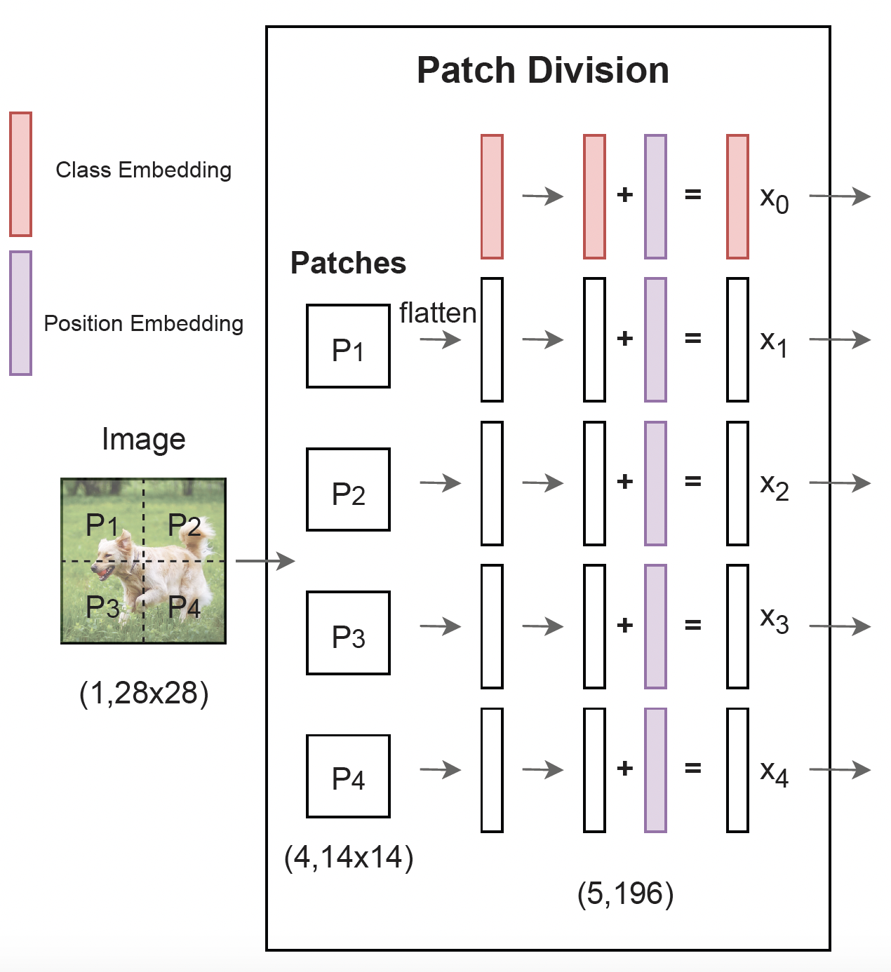
Figure 2: Patch division part of the transformer network for an image split into four patches. Note Class Embedding and Position Embedding are trainable vectors. DBK⁺ (20).

Next, feature extraction is performed using a transformer layer VSP⁺ (17); DBK⁺ (20) which is repeated $L$ times, as shown in Fig.3. Within the transformer layer, we first apply layer normalisation over all patches $x_{i}$, and then apply the attention mechanism detailed in Fig.4. After this part, we obtain a state to which we add the initial input vectors before normalisation in an operation called residual layer, represented by the blue arrow in Fig.3, followed by another layer normalisation. After this, we apply a Multi Layer Perceptron (MLP), which consists of multiple fully connected linear layers for each vector that result in same-sized vectors. Again, we add the residual from just before the last layer normalisation, which is the output of one transformer layer.

After repeating the transformer layer $L$ times, we finally take the vector corresponding to the class embedding, that is the vector corresponding to $x_{0}$, in the final output and apply a fully connected layer of dimension ($d$ $\times$ number of classes) to provide the final classification result (see Fig.1). It is important to observe here that we only use the first vector outcome in the final fully connected layer to do the classification (therefore the name ”class embedding”).

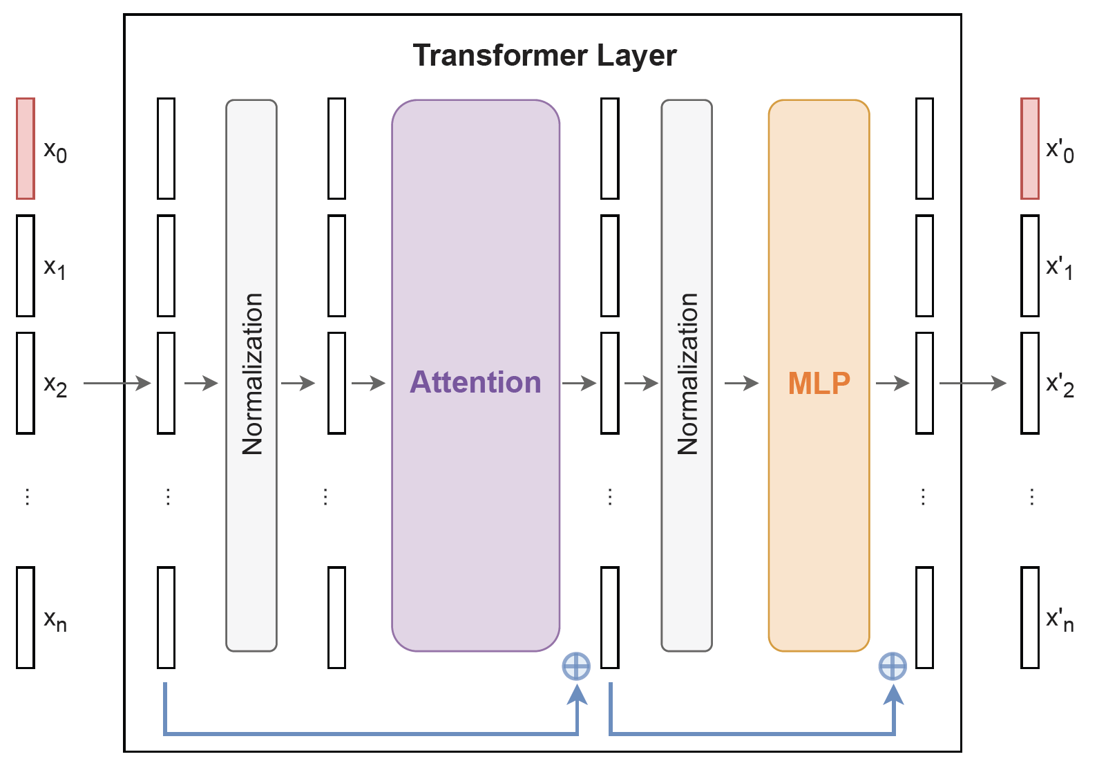
Figure 3: Single transformer layer. DBK⁺ (20).

Looking inside the attention mechanism (see Fig.4), we start by using a fully connected linear layer with trainable weights $V$ to calculate for each patch $x_{i}$ the feature vector $Vx_{i}$. Then to calculate the attention coefficients, we use another trainable weight matrix $W$ and define the attention given by patch $x_{i}$ to patch $x_{j}$ as $x_{i}^{T}Wx_{j}$. Next, for each patch $x_{i}$, we get the final extracted features as the weighted sum of all feature vectors $Vx_{j}$ where the weights are the attention coefficients. This is equivalent to performing a matrix multiplication with a matrix $A$ defined by $A_{ij}=x_{i}^{T}Wx_{j}$. Note, in classical transformer architecture, a column-wise softmax is applied to all $A_{ij}$ and attention coefficients $A^{\prime}_{ij}=softmax_{j}(A_{ij})$ is used instead. Overall, the attention mechanism makes use of $2d^{2}$ trainable parameters, evenly divided between $V$ and $W$.

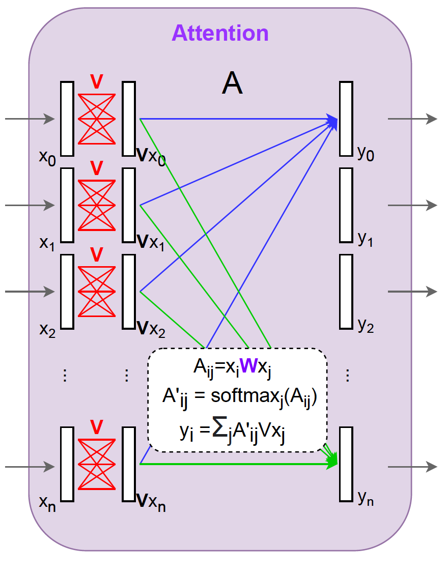
Figure 4: The attention mechanism at the heart of the transformer layer. Matrices $V$ and $W$ are trainable.

In fact, the above description is a slight variant from the original transformers proposed in VSP⁺ (17), where the authors used two trainable matrices to obtain the attention coefficients instead of one ($W$) in this work. This choice was made to simplify the quantum implementation but could be extended to the original proposal using the same quantum tools.

Computational complexity of classical attention mechanism depends mainly on the number of patches $n$ and their individual dimension $d$: the first patch-wise matrix multiplication with the matrix $V\in\mathbb{R}^{d\times d}$ takes $O(nd^{2})$ steps, while the subsequent multiplication with the large matrix $A^{\prime}$ takes $O(n^{2}d)$. Obtaining $A^{\prime}$ from $W$ requires $O(nd^{2})$ steps as well. Overall, the complexity is $O(nd^{2}+n^{2}d)$. In classical deep learning literature, the emphasis is made on the second term, which is usually the most costly. Note that a recent proposal KVPF (20) proposes a different attention mechanism as a linear operation that only has a $O(nd^{2})$ computational complexity.

We compare the classical computational complexity with those of our quantum methods in Table 2. These running times have an real impact on both training and inference, as they measure how the time to perform each layer scales with the number and dimension of the patches.

III Quantum Tools

III.1 Quantum Data Loaders for Matrices

In order to perform a machine learning task with a quantum computer, classical data (a vector, a matrix) needs to be loaded into the quantum circuit. The technique we choose for this task is called amplitude encoding, which uses the classical scalar component of the data as amplitudes of a quantum state made of $d$ qubits. In particular we build upon previous methods to define quantum data loaders for matrices, as shown in Fig.6.

In previous work JDM⁺ (21), we detailed how to perform such data loading for vectors. JDM⁺ (21) proposed three different circuits to load a vector $x\in\mathbb{R}^{d}$ using $d-1$ gates for a circuit depth ranging from $O(log(d))$ to $O(d)$ as desired (see Fig.5). These data loaders use the unary amplitude encoding, where a vector $x=(x_{1},\cdots,x_{d})$ is loaded in the quantum state $\mathinner{|{x}\rangle}=\frac{1}{\left\lVert x\right\rVert}\sum_{i=1}^{d}x_{i}\mathinner{|{e_{i}}\rangle}$ where $\mathinner{|{e_{i}}\rangle}$ is the quantum state with all qubits in $0$ except the $i^{th}$ one in state $1$ (e.g. $\mathinner{|{0\cdots 010\cdots 0}\rangle}$). The circuit uses $RBS$ gates: a parametrised two-qubit gate given by the following unitary matrix:

$$RBS(\theta)=\left(\begin{array}[]{cccc}1&0&0&0\\ 0&\cos\theta&\sin\theta&0\\ 0&-\sin\theta&\cos\theta&0\\ 0&0&0&1\end{array}\right)$$ (1)

The $d-1$ parameters $\theta_{i}$ of the RBS gates are classically pre-computed to ensure that the output of the circuit is indeed $\mathinner{|{x}\rangle}$.

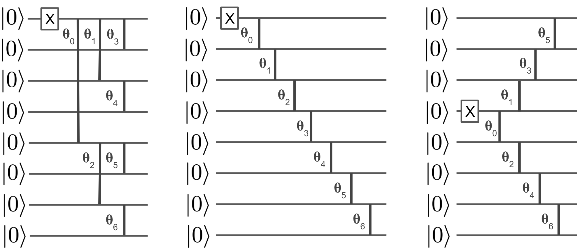
Figure 5: Three possible data loaders for $d$-dimensional vectors ($d=8$). From left to right: the parallel, diagonal, and semi-diagonal circuit have respectively a circuit depth of $log(d)$, $d$, and $d/2$. The X gate represent the Pauli X gate, and the vertical lines represent $RBS$ gates with tunable parameters.

In this work, a data loader for matrices is required. Given a matrix $X\in\mathbb{R}^{n\times d}$, instead of loading a flattened vector, rows $X_{i}$ are loaded in superposition. As shown in Fig.6, on the top qubit register, we first load the vector $(\left\lVert X_{1}\right\rVert,\cdots,\left\lVert X_{n}\right\rVert)$ made of the norms of each row, using a data loader for a vector and obtain a state $\frac{1}{\left\lVert X\right\rVert}\sum_{i=1}^{n}\left\lVert X_{i}\right\rVert\mathinner{|{e_{i}}\rangle}$. Then, on a lower register, we are sequentially loading each row $X_{i}\in\mathbb{R}^{d}$. To do so, we use vector data loaders and their adjoint, as well as CNOTs controlled on the $i^{th}$ qubit of the top register. The resulting state is a superposition of the form:

$$\mathinner{|{X}\rangle}=\frac{1}{\left\lVert X\right\rVert}\sum_{i=1}^{n}\sum_{j=1}^{d}X_{ij}\mathinner{|{e_{j}}\rangle}\mathinner{|{e_{i}}\rangle}$$ (2)

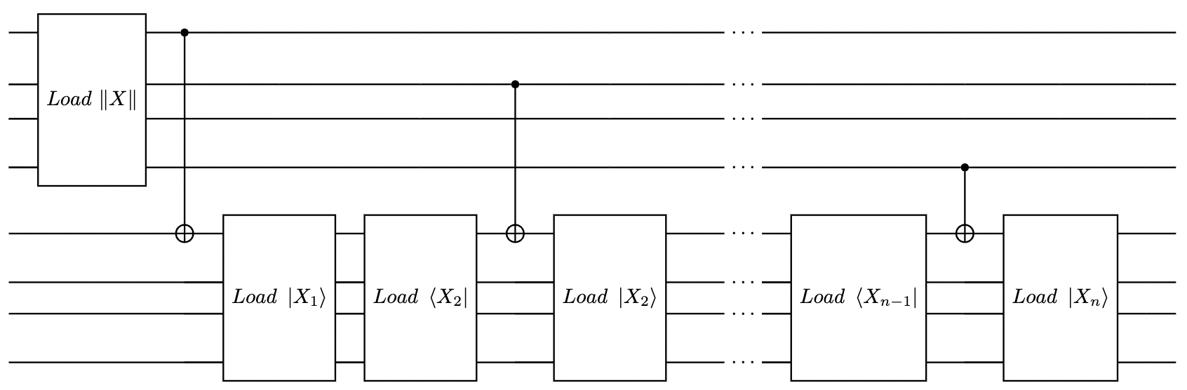
Figure 6: Data loader circuit for a matrix $X\in\mathbb{R}^{n\times d}$. The top register uses $n$ qubits to load the norms of the rows. The lower register uses $d$ qubits to load all rows sequentially, by applying the loader and their adjoint for each row $X_{i}$, with CNOTs controlled by the corresponding qubit $i$ of the top register. Each loader on the lower register has depth $O(\log d)$.

One immediate application of data loaders that construct amplitude encodings is the ability to perform fast inner product computation with quantum circuits. Applying the inverse data loader of $x_{i}$ after the regular data loader of $x_{j}$ effectively creates a state of the form $\braket{x_{i},x_{j}}\mathinner{|{e_{1}}\rangle}+\mathinner{|{G}\rangle}$ where $\mathinner{|{G}\rangle}$ is a garbage state. The probability of measuring $\mathinner{|{e_{1}}\rangle}$, which is simply the probability of having a $1$ on the first qubit, is $|\braket{x_{i},x_{j}}|^{2}$. Techniques to retrieve the sign of the inner product have been developed in MLL⁺ (21).

Loading a whole matrix in a quantum state is a powerful technique for machine learning. However, for large matrices, it requires dee quantum circuits, especially in case of large $n$, thus making this technique more suited for larger quantum computers.

III.2 Quantum Orthogonal Layers

In this section, we outline the concept of Quantum Orthogonal Layers used in neural networks, which generalises the work in KLM (21). These layers correspond to parametrised circuits of $n$ qubits made of $RBS$ gates. More generally, RBS gates preserve the number of ones and zeros in any basis state: if the input to a quantum orthogonal layer is a vector in unary amplitude encoding, the output will be another vector in unary amplitude encoding. Similarly, if the input quantum state is a superposition of only basis states of hamming weight 2, so is the output quantum state. This output state is precisely the result of a matrix-vector product, where the matrix is the unitary matrix of the quantum orthogonal layer, restricted to the basis used. Therefore, for unary basis, we consider a $n\times n$ matrix $W$ instead of the full $2^{n}\times 2^{n}$ unitary. Similarly for the basis of hamming weight two, we can restrict the unitary to a $n\choose 2$ $\times$ $n\choose 2$ matrix. Since the reduced matrix conserves its unitary property and has only real values, these are orthogonal matrices. Each element $W_{ij}$ of the orthogonal matrix $W$ can be seen as the weight of all paths that map state $\mathinner{|{e_{j}}\rangle}$ to state $\mathinner{|{e_{i}}\rangle}$, as explained in previous work KLM (21). More generally, we can think of such hamming weight preserving circuits with $n$ qubits as block-diagonal unitaries that act separately on $n+1$ subspaces, where the $k$-th subspace is defined by all computational basis states with hamming weight equal to $k$. The dimension of these subspaces is equal to $n\choose k$.

There exist many possibilities for building a Quantum Orthogonal Layer, each with different properties. In KLM (21), we proposed the Pyramid circuit shown in Fig.7, composed of exactly $n(n-1)/2$ $RBS$ gates in pyramid-shaped layout. This circuit requires only adjacent qubit connectivity, which is the case for most superconducting qubit hardware. More precisely, the set of matrices that are equivalent to the Quantum Orthogonal Layers with pyramidal layout is exactly the Special Orthogonal Group, made of orthogonal matrices with determinant equal to $+1$. We have showed that by adding a final $Z$ gate on the last qubit would allow having orthogonal matrices with $-1$ determinant. The pyramid circuit is therefore very general and cover all the possible orthogonal matrices of size $n\times n$.

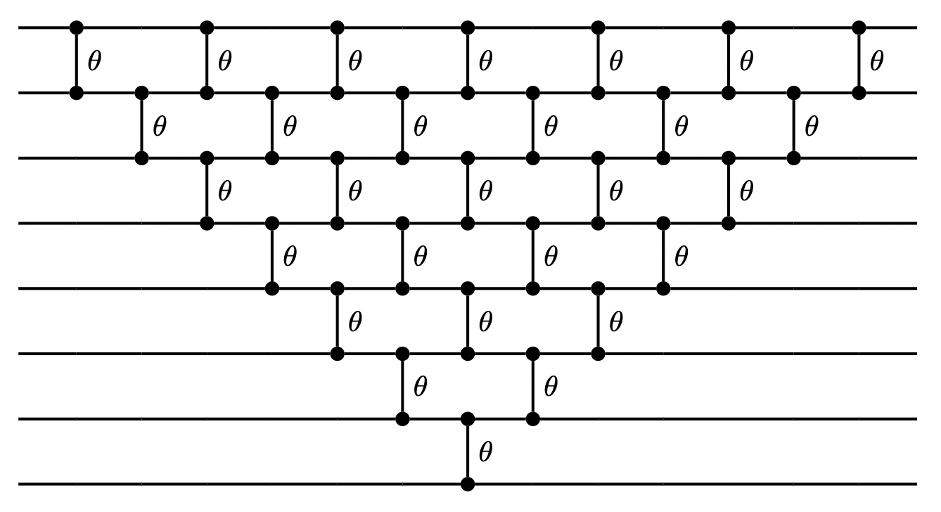
Figure 7: Pyramid circuit on 8 qubits. Each vertical bar is a two qubits $RBS$ gate with an independent parameter $\theta_{i}$.

In this work, we introduce two new types of Quantum Orthogonal Layers: the butterfly circuit (Fig.9), and the $X$ circuit (Fig.9). The $X$ circuit requiring smaller number of gates is the most suited for noisy hardware, since fewer gates imply less error, while retaining the property that there exists a path from every input qubit to every output qubit. Given the smaller number of gates required, the $X$ circuit is less expressive since the set of possible orthogonal matrices is restrained, having fewer free parameters. The butterfly circuit has the very interesting property of having logarithmic depth, a linear number of gates, retaining high level of expressivity. It originated from the classical Cooley–Tukey algorithm CT (65), used for Fast Fourier Transform. Note that this circuit requires the ability to apply the RBS gates on all qubit pairs.

In previous work KLM (21), we have shown that there exists a method to compute the gradient of each parameter $\theta_{i}$ in order to update them. This backpropagation method for the pyramid circuit takes time $O(n^{2})$, corresponding to the number of gates, and provided a polynomial improvement in run time compared to the previsously known orthogonal neural network training algorithms JLW⁺ (19). The exact same method developed for the pyramid circuit can be used to perform quantum backpropagation on the new circuits introduced in this paper. The run time also corresponds to the number of gates, which is lower for the butterfly and $X$ circuits. See for full details on the comparison between the three types of circuits.

Circuit	Hardware Connectivity	Depth	# Gates
Pyramid	NN	$2n-3$	$\frac{n(n-1)}{2}$
X	NN	$n-1$	$2n-3$
Butterfly	All-to-all	$log(n)$	$\frac{n}{2}log(n)$

Table 1: Comparison of different Quantum Orthogonal Layer circuits with $n$ qubits. NN stands for Nearest Neighbor connectivity.

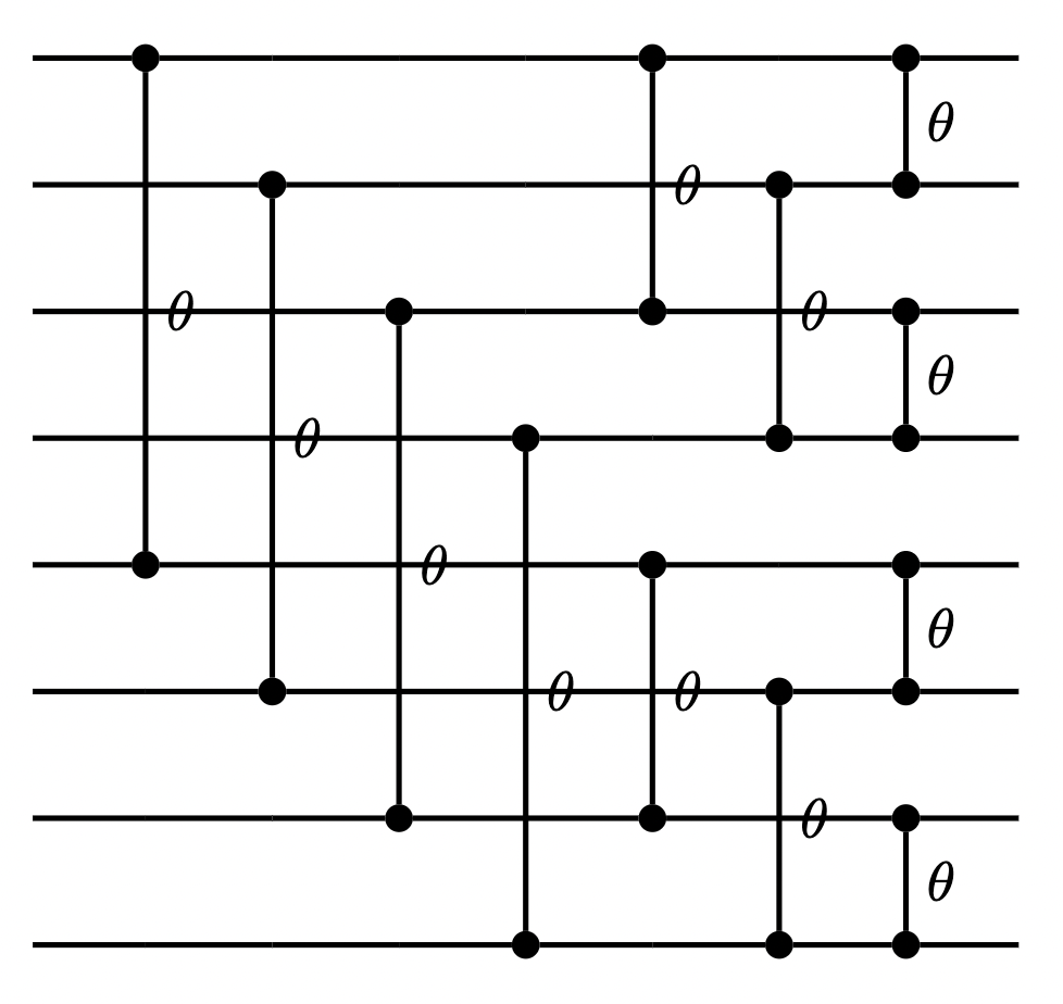
Figure 8: Butterfly Circuit

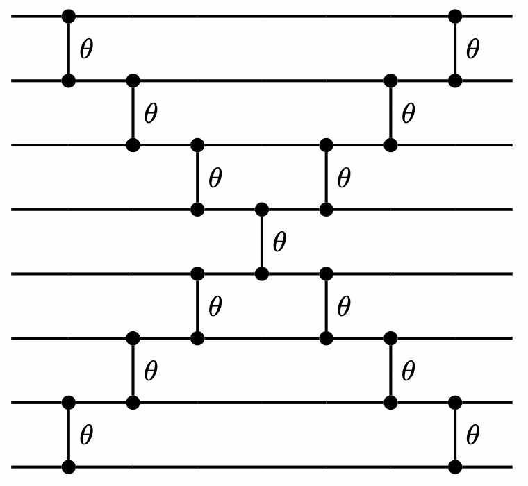
Figure 9: X Circuit

IV Quantum Transformers

Starting from the definition of classical transformers (Section II) and using the quantum tools described above, this section presents several proposals for quantum transformers. Section IV.1 begins, with a simple neural network architecture that serves as the basis for the transformer architectures. In IV.2, quantum circuits for the computation of the attention coefficients are developed, and with this new tool, the quantum Orthogonal Transformer is proposed. In IV.3, an efficient quantum attention mechanism suited for inference is proposed. Finally, in IV.4, a different approach is taken to directly perform the full attention with a new kind of operation more native to quantum linear algebra: the compound matrix multiplication. These last two proposals are very efficient but will require more qubits and larger depth to be implemented as they both use matrix data loading methods. A comparison between these different quantum methods is provided in Table 2, which is applicable to both training and inference.

Algorithm	# Qubits	Circuit depth	# Parametrised Gates	# Distinct circuits
A - Orthogonal Patch-wise	$d$	$O(\log d)$	$O(d\log d)$	$n$
B - Quantum Orthogonal Transformer	$d$	$O(\log d)$	$O(d\log d)$	$n+n^{2}$
C - Quantum Attention Mechanism	$n+d$	$O(\log n+n\log d+\log d)$	$O(d\log d)$	$n$
D - Compound Transformer	$n+d$	$O(\log n+n\log d+\log(n+d))$	$O((n+d)\log(n+d)))$	1

Table 2: Comparison of different quantum methods to perform the attention part of a transformer network. $n$ and $d$ stand respectively for the number of patches and their individual dimension. All Quantum Orthogonal layers are implemented using the butterfly circuits. Note that the classical attention mechanisms require $O(nd^{2}+n^{2}d)$ steps, while the computational complexity of the quantum architectures are reflect in the number of parametrised gates. Both computational complexity and parameter counts are important: the first one for running time, the second one for expressivity and trainability of the network

.

IV.1 Orthogonal Patch-wise Neural Network

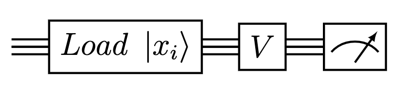
Figure 10: Quantum circuit to perform the matrix multiplication $Vx_{i}$ (fully connected layer) using a data loader for $x_{i}$ and a quantum orthogonal layer for $V$.

First, a simple architecture named orthogonal patch-wise neural network is formulated, which forms the basis of the transformer architectures. As seen in Fig.4, the attention layer is first composed by a series of matrix-vector multiplications: each patch is multiplied by the same trainable matrix $V$.

Building upon the tools developed in Section III, one circuit per patch is used, as shown in Fig.10. Each circuit has $d$ qubits and each patch $x_{i}$ is encoded in a quantum state with a vector data loader. We can use a Quantum Orthogonal Layer (e.g. pyramid, butterfly) to perform a trainable matrix multiplication on each patch. The Quantum Orthogonal Layer is equivalent to a matrix $V$ with a specific structure. The output of each circuit is a quantum state encoding $Vx_{i}$, a vector which is retrieved through tomography. The precision tomography depends on the number of measurements and will be assessed during the numerical simulations.

This network can be thought of as a transformer with a trivial attention mechanism, where each patch pays attention only to itself.

The computational complexity of this circuit is calculated as follows: from Section III.1, a data loader with $d$ qubits has a complexity of $log(d)$ steps. For the orthogonal quantum layer, as shown in Table 1, a butterfly circuit takes $log(d)$ steps as well, with $\frac{d}{2}log(d)$ trainable parameters. Overall, the complexity is $O(log(d))$ and the trainable parameters are $O(d\log d)$.

IV.2 A Quantum Orthogonal Transformer

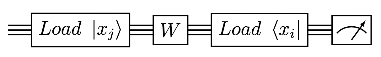
Figure 11: Quantum circuit to compute $|x_{i}^{T}Wx_{j}|^{2}$ (attention coefficients) using data loaders for $x_{i}$ and $x_{j}$ and a quantum orthogonal layer for $W$.

The missing part of the previous architecture is the attention mechanism: the second step described in Fig.4, where all $Vx_{i}$ are combined using attention coefficients $A_{ij}$ to obtain the list of final outputs $y_{j}$.

The attention coefficients used here are defined as $A_{ij}=x_{i}^{T}Wx_{j}$ where $W$ is a trainable matrix. As seen before, the quantum tools perform matrix-vector multiplication using Quantum Orthogonal Layers. As shown in Fig.11, loading any $x_{j}$ with a data loader, followed by a trainable Quantum Orthogonal Layer, is equivalent to encoding $Wx_{j}$. Next, apply the inverse data loader of $x_{i}$, which creates a state where the probability of measuring $1$ on the first qubit is exactly $|x_{i}^{T}Wx_{j}|^{2}$. With classical post-processing, this is enough to retrieve all $A_{ij}$. It is also possible to classically apply a softmax column-wise and obtain $A^{\prime}_{ij}=\text{softmax}_{j}(A_{ij})$ or any other kind of non-linearity. Note the square that appears in the circuit is one type of non-linearity. Using this method, the values of $A$ are always positive, but during the training phase the coefficients are learned nonetheless. Additional methods also exist to obtain the sign of the inner product MLL⁺ (21). The estimation of $A_{ij}$ is repeated each time with a different pair of patches and the same trainable Quantum Orthogonal Layer $W$. The computational complexity of this quantum circuit is similar to the previous one, with one more data loader.

One can now put everything together to have the complete quantum method for training an attention layer: a first set of quantum circuits presented in IV.1 are implemented to obtain each $Vx_{j}$. At the same time, each attention coefficient $|x_{i}^{T}Wx_{j}|^{2}$ is computed, and they are potentially post-processed column wise with softmax to obtain the $A^{\prime}_{ij}$. The two parts can then be classically combined to compute each $y_{i}=\sum_{j}A^{\prime}_{ij}Vx_{j}$. This is the desired output that will be used in the rest of the network. At the end, when the cost function is estimated, backpropagation is used to compute the gradient of each angle of the Quantum Orthogonal Layers (for matrices $V$ and $W$) and update them for the next iteration.

Overall, we presented a quantum Orthogonal Transformer, which is based on quantum transformer layers, whose attention layer has been exchanged for hamming weight preserving parametrised quantum circuits that are trained to provide the weight matrices $V$ and $W$.

IV.3 A Quantum Attention Mechanism

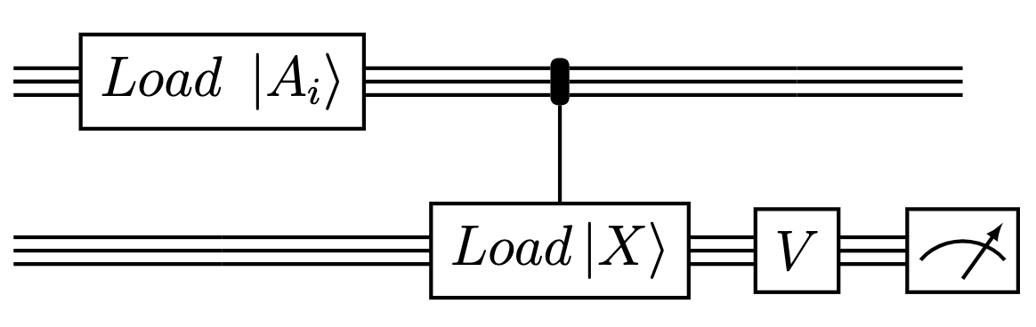
Figure 12: Quantum circuit to perform directly the attention mechanism, assuming the knowledge of the coefficients in $A$. This circuit uses a quantum orthogonal layer for $V$. Before this, the circuit corresponds to the matrix data loader from Fig.6, where $Load(\left\lVert X\right\rVert)$ is replaced by $Load(A_{i})$.

In the previous section, the output of the attention layer $y_{i}=\sum_{j}A^{\prime}_{ij}Vx_{j}$ was computed classically once the quantities $A^{\prime}_{ij}$ and $Vx_{j}$ had been computed with the help of quantum circuits.

Here, the quantum attention mechanism is implemented more directly with a quantum circuit, which can be used during inference. Consider that the matrices $V$ and $W$ have been trained before, and the attention matrix $A$ (or $A^{\prime}$) is stored classically. The goal is to compute each $y_{i}=\sum_{j}A_{ij}Vx_{j}$ using a global quantum circuit. For this, the use of the matrix data loader from Fig.6 is used.

In Fig.12, we show how for each patch with index $i$, we can use a quantum circuit whose qubits are split into two main registers. On the top register, the vector $A_{i}$ is loaded via a vector data loader, i.e. the $j^{th}$ column of the attention matrix $A$ (or $A^{\prime}$) which is assumed to be normalized. At this stage, the quantum state obtained is:

$$\sum_{j}A_{ij}\mathinner{|{e_{j}}\rangle}\mathinner{|{0}\rangle}$$ (3)

Now an operation is performed similar to the matrix data loader of Fig.6: the data loader and its adjoint of vector $x_{i}$ are applied sequentially on the lower register, with CNOTs controlled on each qubit $i$ of the top register. This gives the following quantum state:

$$\begin{split}\sum_{j}A_{ij}\mathinner{|{e_{j}}\rangle}\mathinner{|{x_{j}}\rangle}\end{split}$$ (4)

Another way to see this is that the matrix $X$ is loaded with all rows re-scaled according to the attention coefficients.

The last step consists of applying the Quantum Orthogonal Layer $V$ that has been trained before on the second register of the circuit. As previously established, this operation performs matrix multiplication between $V$ and the vector encoded on the second register. Since the $k^{th}$ element of the vector $Vx_{j}$ can be written as $\sum_{q}V_{kq}x_{jq}$, we have:

$$\begin{split}\sum_{j}A_{ij}\mathinner{|{e_{j}}\rangle}\mathinner{|{Vx_{j}}\rangle}\\ =\sum_{j}A_{ij}\mathinner{|{e_{j}}\rangle}\sum_{k}(\sum_{q}V_{kq}x_{jq})\mathinner{|{e_{k}}\rangle}\\ =\sum_{k}\sum_{j}A_{ij}(\sum_{q}V_{kq}x_{jq})\mathinner{|{e_{j}}\rangle}\mathinner{|{e_{k}}\rangle}\end{split}$$ (5)

Since $y_{i}=\sum_{j}A_{ij}Vx_{j}$, its $k^{th}$ element can be written $y_{ik}=\sum_{j}A_{ij}(\sum_{q}V_{kq}x_{jq})$. Therefore, the quantum state at the end of the circuit can be written as $\mathinner{|{y_{i}}\rangle}=\sum_{k}y_{ik}\mathinner{|{\phi_{k}}\rangle}\mathinner{|{e_{k}}\rangle}$ for some normalised states $\mathinner{|{\phi_{k}}\rangle}$ which by performing tomography on the second register can give us the output vector $y_{i}$.

This circuit is therefore a more direct method to compute each $y_{i}$, and is repeated for each $y_{i}$, using a different $A_{i}$ in the first loader. As shown in Table 2, compared with the previous method, this method requires fewer quantum circuits to run, but each circuit requires more qubits and a deeper circuit.

To analyse the computational complexity: the first data loader on the top register has $n$ qubit and $\log n$ depth; the following $2n$ loaders on the bottom register have $d$ qubits and $2n\log d$ depth; and the final quantum orthogonal layer $V$ implemented using a butterfly circuit, has a depth of $\log d$ and $O(d\log d)$ trainable parameters.

IV.4 A Quantum Compound Transformer

So far, we follow quite closely the steps of a classical transformer by using quantum linear algebra procedures to reproduce each step with a few deviations. The same quantum tools can also be used in a more natively quantum fashion, while retaining the spirit of classical transformers, as shown in Fig.13.

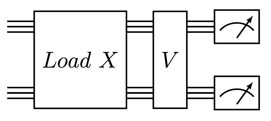
Figure 13: Quantum circuit to perform a compound transformer. We use a matrix dataloader for $X$ (equivalent to Fig.6) and a quantum orthogonal layer for $V$ applied on both registers.

This quantum circuit has two registers: the top one of size $n$ and the bottom one of size $d$. The full matrix $X\in\mathbb{R}^{n\times d}$ is loaded into the circuit using the matrix data loader from Section III.1 with $n+d$ qubits. This could correspond to the entire image, as every image can be split into $n$ patches of size $d$ each. We then apply a Quantum Orthogonal Layer on the two registers at the same time. As explained in Section III.2, this hamming weight preserving quantum circuit should be seen as a multiplication with an orthogonal matrix of size $(n+d)\times(n+d)$, if the input state is a unary encoding. In the case of the Compound Transformer, we are stepping out of this unary framework. Here, the top qubits encode the norms of each vector using the matrix data loader, and the overall state over both registers is a superposition of states of hamming weight two (exactly two qubits are in state 1). Note that not all states of hamming weight two, whose number is $\binom{n+d}{2}$, are part of this superposition, but only $n\times d$ of them, which correspond to states with one 1 in the first $n$ qubits, and another 1 in the remaining $d$ qubits.

The operation performed in this circuit is a matrix-vector multiplication in a space of dimension $\binom{n+d}{2}$, where each dimension corresponds to a computational basis with hamming weight 2 KP (22). Note that $V$ and $X$ are not a priori in this dimension. $X$ as a $n\times d$ vector need first be transformed into a vector of size $\binom{n+d}{2}$ by adding zeros to all dimensions that correspond to computational basis vectors that have both 1s on the top $n$ qubits or bottom $d$ qubits. Next, a matrix $\mathcal{V}^{(2)}$ of size $\binom{n+d}{2}\times\binom{n+d}{2}$ called the $2^{nd}$ order compound matrix of $V$ can be computed.

Given a matrix $A\in\mathbb{R}^{n\times n}$, the $k^{th}$-compound matrix $\mathcal{A}^{(k)}$ for $k\in[n]$ is the $\binom{n}{k}$ dimensional matrix with entries $\mathcal{A}^{(k)}_{IJ}=det(A_{IJ})$ where $I$ and $J$ are subsets of rows and columns of $A$ with size k. In the present case, the $2^{nd}$ order compound matrix uses $k=2$, and each entry of $\mathcal{V}^{(2)}$ is the determinant of a $2\times 2$ submatrix that corresponds to the intersection of 2 rows and 2 columns of $V$.

Thus, simulating the application of the quantum circuit $V$ on an input state that corresponds to a $n\times d$ matrix $X$ corresponds to performing a matrix-vector multiplication of dimension $\binom{n+d}{2}$, which takes $O((n+d)^{4})$ time. More generally, this compound matrix operation on an arbitrary input state of hamming weight $k$ is quite hard to perform classically, since all determinants must be computed, and a matrix-vector multiplication of size $\binom{n+d}{k}$ needs to be applied.

These properties of the compound matrix operation are used to define a new quantum attention layer of dimension ${(n\times d)}\times{(n\times d)}$. As shown in Fig.13, the input to the circuit is a matrix $X\in\mathbb{R}^{n\times d}$ which corresponds to the patches of an image. The matrix data loader creates the state $\mathinner{|{X}\rangle}$, and after applying the quantum orthogonal layer on all $n+d$ qubits, the resulting state is $\mathinner{|{Y}\rangle}=\mathinner{|{\mathcal{V}^{(2)}X}\rangle}$, where $\mathcal{V}^{(2)}$ is the $2^{nd}$-order compound matrix of $V$ defined above. As mentioned above, this state has dimension $\binom{n+d}{2}$, i.e. there are exactly two 1s in the $(n+d)$ qubits, but one can postselect only the part of the state where there is exactly one qubit in state 1 on the top register and the other 1 on the lower register. This way, $n\times d$ output states are generated. In other words, tomography is performed for a state of the form $\mathinner{|{Y}\rangle}=\frac{1}{\left\lVert Y\right\rVert}\sum_{i=1}^{n}\sum_{j=1}^{d}y_{ij}\mathinner{|{e_{j}}\rangle}\mathinner{|{e_{i}}\rangle}$ which is used to conclude that this quantum circuit produces transformed patches $(y_{1},\cdots,y_{n})\in\mathbb{R}^{n\times d}$.

For the complexity of this circuit we have: the matrix data loader, detailed in Fig.6 has depth of $\log n+2n\log d$; the Quantum Orthogonal Layer applied on $n+d$ qubits has a depth $log(n+d)$ and $(n+d)log(n+d)$ trainable parameters implemented using butterfly circuit.

Overall, this simple circuit can replace both the patch-wise (IV.1) and the attention layer (IV.2) defined before, as a combined operation. The use of compound matrix multiplication is different from usual transformers, but still share some interesting properties: patches are weighted in its global context and share gradients through the determinants. One can say that the Compound Transformer operates in a similar spirit as the MLPMixer architecture presented in THK⁺ (21). This state-of-the-art architecture used for image classification tasks mixes the different patches without using convolution or attention mechanisms. The underlying mechanism operates in two steps by first mixing the patches and then extracting the patch-wise features using fully connected layers. Similarly, the Compound Transformer performs both steps at the same time.

V Medical Image Classification via Quantum Transformers

V.1 Datasets

In order to benchmark our models, we used MedMNIST, a collection of 12 preprocessed, two-dimensional medical image open datasets YSN (20); YSW⁺ (21). The collection has been standardised for classification tasks on 12 different imaging modalities, each with medical images of $28\times 28$ pixels. We used our transformers to do simulations on all 12 MedMNIST datasets. For the hardware experiments, we focused on one of them, RetinaMNIST. The MedMNIST dataset was chosen for our benchmarking efforts due to its accessible size for simulations of the quantum circuits and hardware experiments, while being representative of one important field of computer vision application: classification of medical images.

V.2 Simulations

Network	PathMNIST		ChestMNIST		DermaMNIST		OCTMNIST		PneumoniaMNIST		RetinaMNIST
	AUC	ACC	AUC	ACC	AUC	ACC	AUC	ACC	AUC	ACC	AUC	ACC
VisionTransformer DBK+ (20)	0.957	0.755	0.718	0.948	0.895	0.727	0.879	0.608	0.957	0.902	0.736	0.548
OrthoFNN KLM (21)	0.939	0.643	0.701	0.947	0.883	0.719	0.819	0.516	0.950	0.864	0.731	0.548
OrthoPatchWise	0.953	0.713	0.692	0.947	0.898	0.730	0.861	0.554	0.945	0.867	0.739	0.560
OrthoTransformer	0.964	0.774	0.703	0.947	0.891	0.719	0.875	0.606	0.947	0.885	0.745	0.542
CompoundTransformer	0.957	0.735	0.698	0.947	0.901	0.734	0.867	0.545	0.947	0.885	0.740	0.565
Network	BreastMNIST		BloodMNIST		TissueMNIST		OrganAMNIST		OrganCMNIST		OrganSMNIST
	AUC	ACC	AUC	ACC	AUC	ACC	AUC	ACC	AUC	ACC	AUC	ACC
VisionTransformer DBK+ (20)	0.824	0.833	0.985	0.888	0.880	0.596	0.968	0.770	0.970	0.787	0.934	0.620
OrthoFNN KLM (21)	0.815	0.821	0.972	0.820	0.819	0.513	0.916	0.636	0.923	0.672	0.875	0.481
OrthoPatchWise	0.830	0.827	0.984	0.866	0.845	0.549	0.973	0.786	0.976	0.805	0.941	0.640
OrthoTransformer	0.770	0.744	0.982	0.860	0.856	0.557	0.968	0.763	0.973	0.785	0.946	0.635
CompoundTransformer	0.859	0.846	0.985	0.870	0.841	0.544	0.975	0.789	0.978	0.819	0.943	0.647

Table 3: Performance analysis using AUC and ACC on each test dataset of MedMNIST of our quantum architectures (Orthogonal PatchWise, Orthogonal Transformer and Compound Transformer) compared to the classical (Vision Transformer DBK⁺ (20)) and quantum (Orthogonal FNN MLL⁺ (21)) baselines

described in Section V.

First, simulations of our models are performed on the 2D MedMNIST datasets and demonstrate that the proposed quantum attention architecture reaches accuracy comparable to and at times better than the various standard classical models. Next, the setting of our simulations are described and the results compared against those reported in the AutoML benchmark performed by the authors in YSW⁺ (21).

V.2.1 Simulation setting MedMNIST

In order to benchmark the performance of the three different quantum transformer mechanisms described in this work, namely, Orthogonal Patch-wise from Section IV.1, Orthogonal Transformer from Section IV.2, and Compound Transformer from Section IV.4, the complete training procedure of the multiple quantum circuits that compose each network was simulated. Moreover, two baseline methods have been included in the benchmark. The first baseline is the Vision Transformer, described in Section II (DBK⁺ (20)), which is a classical neural network that has been applied to different image classification tasks. The second baseline is the Orthogonal Fully-Connected Neural Network (OrthoFNN), a quantum method that has been trained on the RetinaMNIST dataset in MLL⁺ (21).

To ensure comparable evaluations between the five neural networks, similar architectures were implemented for all five. The chosen architecture comprises of three parts: pre-processing, features extraction, and post-processing. The first part is classical and pre-processes the input image of size $28\times 28$ by extracting $16$ patches of size $7\times 7$. We then map every patch to the dimension of the feature extraction part of the neural network, by using a fully connected neural network layer. We have experimented with dimensions of $16$, $32$ and $64$ for the size of these layers, but a dimension of $16$ was providing accurate results and had the smallest number of parameters, so we report here those results. Note that this first pre-processing fully connected layer is trained in conjunction to the rest of the architecture. For the OrthoNN networks, used as our quantum baseline, patches of size $16$ were extracted from the complete input image using a fully connected neural network layer of size $784\times 16$. This fully connected layer is trained in conjunction to the quantum circuits.

The second part of the common architecture transforms the extracted features by applying a sequence of layers, specific to every architecture, on the extracted patches. Every sequence is made with $4$ layers that maintain the dimension of the neural network. Moreover, the same gate layout, the butterfly circuit, is used for all circuits that compose the quantum layers. Finally, the last part of the neural network is classical, which linearly projects the extracted features and outputs the predicted label.

The JAX package BFH⁺ (18) was used to efficiently simulate the complete training procedure of the five benchmark architectures. The experimental hyperparameters used in YSW⁺ (21) were replicated for our benchmark: every model is trained using the cross-entropy loss with the Adam optimiser KB (15) for $100$ epochs, with batch size of $32$ and a learning rate of $10^{-3}$ that is decayed by a factor of $0.1$ after $50$ and $75$ epochs.

V.2.2 Simulation results MedMNIST

The 5 different neural networks were trained over $3$ random seeds, and the best overall performance for each one of them was selected. The evaluation procedure is similar to the AutoML benchmark in YSN (20); YSW⁺ (21), and the benchmark results are shown in Table 3 where the area under receiver operating characteristic (ROC) curve (AUC) and the accuracy (ACC) are reported as evaluation metrics. A full comparison with the classical benchmark provided by YSN (20) is given in (Appendix A, Table 6).

Circuit	Qubits	RBS Gates for Loaders (Fixed Parameters)	RBS Gates for Orthogonal Layers (Trainable Parameters)
Orthogonal PatchWise	16	15	32
Orthogonal Transformer	16	45	64
Compound Transformer	32	480	80

Table 4: Resource analysis for the MedMNIST simulations shown in Table 3. The number of required qubits, the total number of parametrised gates with fixed parameters, and with trainable parameters for each quantum network are shown. These numbers are to be compared with the 512 trainable parameters per layer of the classical Vision Transformers. These simulations were performed for 16 patches per image with 16 features per patch and used the butterfly circuits as the orthogonal layer. The Orthogonal Transformer uses two types of quantum circuits: one to perform the operation $Vx_{i}$ and one to perform the operation $x_{i}^{T}Wx_{j}$, which respectively use the resources mentioned. Note that the Compound Transformer scales more harshly with respect to number of gates required for data loading, but compensates with lowers the number of required circuits as a trade off.

From Table 3, we observe that Quantum Orthogonal and Compound Transformer architectures outperform the Orthogonal Fully-Connected and Orthogonal Patch-wise neural networks most of the time. This may be due to the fact that the latter do not rely on any mechanism that exchange information across the patches. Second, all quantum neural networks provide very competitive performances compared to the AutoML benchmark and outperform their classical counterparts on 7 out of 12 MedMNIST datasets.

Moreover, comparisons can be made with regard to the number of parameters used by each architecture, in particular for feature extraction. Table 4 presents a resource analysis for the quantum circuits that were simulated, per layer. It includes the number of qubits, the number of gates with trainable parameters, and the number of gates with fixed parameters used for loading the data. The table shows that our quantum architectures have a small number of trainable parameters per layer. The global count for each quantum method is as follows.

• Orthogonal Patch-wise Neural Network: $32$ parameters per circuit, 16 circuits per layer which use the same 16 parameters, and 4 layers, for a total of $128$ trainable parameters.

• Quantum Orthogonal Transformer: $32$ parameters per circuit, $17$ circuits which use the same 16 parameters and another $289$ circuits which use another set of 16 parameters per layer, and 4 layers, for a total of $256$ trainable parameters.

• Compound Transformer: $80$ parameters per circuit, 1 circuit per layer, and 4 layers, for a total of $320$ trainable parameters.

These numbers are to be compared with the number of trainable parameters in the classical Vision Transformer that is used as a baseline. As stated in Section II, each classical attention layer requires $2d^{2}$ free parameters, which in the simulations performed here corresponds to 512, making the total trainable parameters used in attention layer in the classical Vision Transformer 2064. Note again this resource analysis focuses on the attention layer of the each transformer network, and does not include parameters used for the preprocessing of the images (see Section V.2.1), as part of other transformer layers (Fig.3), and for the single layer used in the final classification (Fig.1), which are common in all cases.

More generally, performance of other classical neural network models provided by the authors of MedMNIST is compared to our approaches in Table 6 found in the Appendix. Some of these classical neural networks reach somewhat better levels of accuracy, but are known to use an extremely large number of parameters. For instance, the smallest reported residual network has approximately a total number of $10^{7}$ parameters, and the automated machine learning algorithms train numerous different architectures in order to reach that performance.

Based on the results of the simulations in this section, quantum transformers are able to train across a number different of classification tasks, deliver performances that are highly competitive and sometimes better than the equivalent classical methods.

V.3 Quantum Hardware Experiments

Quantum hardware experiments were performed on one specific dataset: RetinaMNIST. It has $1080$ images for training, $120$ images for validation, and $400$ images for testing. Each image contains $28\times 28$ RGB pixels. Each image is classified into 1 of 5 classes (ordinal regression).

V.3.1 Hardware Description

The hardware demonstration was performed on two different superconducting quantum computers provided by IBM, with the smaller experiments performed on the 16-qubit ibmq_guadalupe machine (see Fig.14) and the larger ones on the 27-qubit ibm_hanoi machine. Results are reported here from experiments with four, five and six qubits; experiments with higher numbers of qubits, which entails higher numbers of gates and depth, did not produce meaningful results.

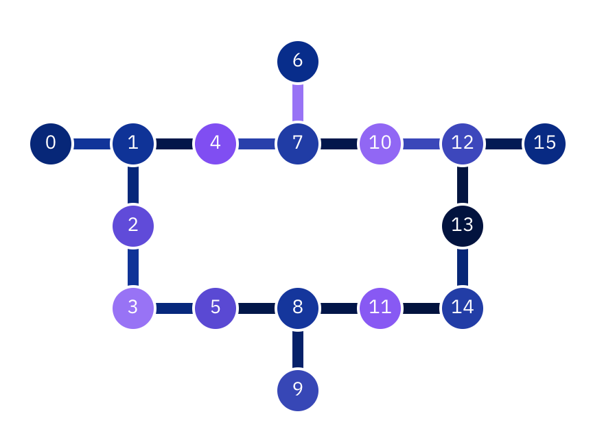
Figure 14: Connectivity of the 16-qubit ibmq_guadalupe quantum computer.

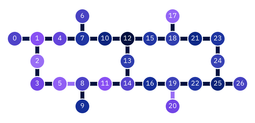
Figure 15: Connectivity of the 27-qubit ibm_hanoi quantum computer.

Note that the main sources of noise are the device noise and the finite sampling noise. In general, noise is undesirable during computations. In the case of a neural network, however, noise may not be as troublesome: noise can help escape local minima NYMH (17), or act as data augmentation to avoid over-fitting. In classical deep learning, noise is sometimes artificially added for these purposes Yin (19). Despite this, when the noise is too large, we also see a drop in the accuracy.

V.3.2 Hardware Results

Model	Classical (JAX)		IBM Simulator		IBM Hardware
	AUC	ACC	AUC	ACC	AUC	ACC
Google AutoML (Best in YSW+ (21))	0.750	53.10 %	-	-	-	-
VisionTransformer (our classical benchmark)	0.736	55.75 %	-	-	-	-
OrthoPatchWise (Pyramid Circuit)	0.738	56.50 %	0.731	54.75 %	0.727	51.75 %
Ortho Transformer (Pyramid Circuit)	0.729	55.00 %	0.715	55.00 %	0.717	54.50 %
Ortho Transformer with Quantum Attention	0.749	56.50 %	0.743	55.50 %	0.746	55.00 %
CompoundTransformer (X Circuit)	0.729	56.50 %	0.683	56.50 %	0.666	45.75 %
CompoundTransformer ( \ Circuit)	0.716	55.75 %	0.718	55.50 %	0.704	49.00 %

Table 5: Hardware Results for RetinaMNIST using various models. The models were trained for 300-700 epochs on 1080 training images and inferred on 400 test images. Note that “\  Circuit” contains a single diagonal of trainable RBS gates. Classical (JAX): classical code run by JAX, equivalent to quantum operations. IBM Simulator: code compiled to run on actual IBM hardware and executed using their Aer Simulator.

Hardware experiments were performed with four, five and six qubits to push the limits of the current hardware, in terms of both the number of qubits and circuit depth. Three quantum proposals were run: the Orthogonal Patch-wise network (from Section IV.1), the Quantum Orthogonal transformers (from Sections IV and IV.3) and finally the Quantum Compound Transformer (from Section IV.4).

Each quantum model was trained using a JAX-based simulator, and inference was performed on the entire test dataset of $400$ images of the RetinaMNIST on the IBM quantum computers.

The first model, the Orthogonal Patch-wise neural network, was trained using 16 patches per image, 4 features per patch, and one $4\times 4$ orthogonal layer, using a 4-qubit pyramid as the orthogonal layer. The experiment used 16 different quantum circuits of 9 $RBS$ gates per circuit per image. The result was compared with an equivalent classical (non-orthogonal) patch-wise neural network, and a small advantage in accuracy for the quantum native method could be reported.

The second model, the Quantum Orthogonal Transformer, used $4$ patches per image, 4 features per patch, and an attention mechanism with one $4\times 4$ orthogonal layer and trainable attention coefficients. 4-qubit pyramids were used as orthogonal layers. The experiment used 25 different quantum circuits of 12 $RBS$ gates per circuit per image and 15 different quantum circuits of 9 $RBS$ gates per circuit per image.

The third set of experiments ran the Orthogonal Transformer with the quantum attention mechanism. We used $4$ patches per image, 4 features per patch, and a quantum attention mechanism that paid attention to only the neighbouring patch, thereby using a $5$-qubit quantum circuit with the $X$ as the orthogonal layer. The experiment used 12 different quantum circuits of 14 $RBS$ gates and 2 $CNOT$s per circuit per image.

The last two quantum proposals were compared with a classical transformer network with a similar architecture and demonstrated similar level of accuracy.

Finally, the fourth experiment was performed on the ibmq_hanoi machine with 6 qubits, with the Compound Transformer, using 4 patches per image, 4 features per patch, and one orthogonal layer using the $X$ layout. The hardware results were quite noisy with the X layer, therefore the same experiments were performed with a further-reduced orthogonal layer named the “\Circuit”: half of a X Circuit (Fig.9) where only one diagonal of $RBS$ gates is kept, and which reduced the noise in the outcomes. The experiment used 2 different quantum circuits of 18 $RBS$ gates and 3 $CNOT$s per circuit per image.

Note that with the restriction to states with a fixed hamming weight, strong error mitigation techniques become available. Indeed, as we expect to obtain only quantum superpositions of unary states or states with hamming weight $2$ in the case of Compound Transformers, at every layer, every measurement can be processed to discard the ones that have a different hamming weight i.e. states with more than one (or two) qubit in state $\mathinner{|{1}\rangle}$. This error mitigation procedure can be applied efficiently to the results of a hardware demonstration, and has been used in the results presented in this paper.

The conclusion from the hardware experiments is that all quantum proposals achieve state-of-the-art test accuracy, comparable to classical networks. In particular, the quantum Compound methods on the simulator are notably more efficient than the classical networks, and they have no efficient classical equivalent. However, the current hardware is often too noisy to achieve similar performance, even with a low number of qubits.

VI Discussion

In this work, quantum approaches for training and forward inference of a vision transformer are presented, with each method tested on a set of image classification tasks. These quantum networks reproduce, more or less closely, the steps that occur in the attention layer of the classical transformers but are quite different from each other. Orthogonal Patchwise is the simplest approach and requires fewer qubits and lower circuit depth. Orthogonal Transformer is the most similar to classical transformers. Compound Transformer steps away from the classical architecture with a quantum native procedure, a linear algebraic operation which that cannot be efficiently done classically: multiplying a vector with a higher-dimensional compound matrix (see definition in Section IV.4).

Inside all these quantum transformers are the Quantum Orthogonal Layers. These trainable circuits can efficiently apply matrix multiplication on vectors encoded on specific quantum basis states. We provide different types of circuits and analyse their advantage in terms of expressivity and complexity. All circuits implement orthogonal matrix multiplication and can be trained using backpropagation detailed in KLM (21). Some circuits have fewer parameters and therefore represent a smaller expressivity but a faster running time. In particular, a quantum computer with all-to-all qubit connectivity can implement the butterfly circuit, which has a logarithmic depth with respect to the equivalent matrix multiplication size.

As shown in Table 2, our quantum circuits show definite advantage in terms of computation complexity of the attention layer. In particular, the Compound Transformer runs quadratically faster than the classical equivalent operation with respect to the dimension and the number of patches, without including preprocessing time. The Compound Transformer also allows for the use of a single circuit instead of many repetitions, but might be more suited for larger quantum computers due its larger depth for data loading.

In addition to theoretical analysis, we performed extensive numerical simulation and quantum hardware experiments to test the quantum circuits on different datasets, and compared them with each other as well as to their classical baselines. Our results show that our quantum circuits can classify the small images correctly, sometimes as well as or better than the state-of-the-art classical methods (see Table 3). Our quantum methods have the potential to address over-fitting issues by using a small number of parameters. While the running time of the fully connected and attention layer has been theoretically proven to be advantageous, this is hard to observe in the current quantum computers due to the limited size, high level of noise, and latency of cloud access.

From our hardware experiments, it can be observed that results from the current hardware become too noisy as soon as the number of qubits or the size of the quantum circuit increased (see Table 5). Hence the exact number of parameters used to run the quantum circuits is expected to change with the availability of larger quantum computers, which will allow for larger quantum operations and for us to forgo classical preprocessing to downsize the input images.

The MedMNIST simulation results show that, in order to provide competitive results, a quantum transformer would need to utilise parametrised quantum circuits with 16 or 32 qubits and between 60 and 600 $RBS$ gates. While the state of the hardware is yet insufficient, our simulation results show a promising level of performance that can be expected once the hardware technology matures.

Overall, our results are encouraging and show the benefit of using quantum circuits that can be trainable but also perform precise linear algebra operations. This approach allows for much better control over the size of the Hilbert space that is explored by the model and provides models that are both expressive and trainable.

VII Acknowledgements

The following members of the Roche pRED Quantum Computing Task Force also contributed to this work: Marielle van de Pol, Timothy Stitt, Betty Tai Lorentzen, Agnes Meyder, Detlef Wolf, Stanislaw Adaszewski, Clemens Wrzodek. We also would like to thank all members of QC Ware who have contributed in the development of the quantum software that was used in this work. We acknowledge the use of IBM Quantum services for this work. The views expressed are those of the authors, and do not reflect the official policy or position of IBM or the IBM Quantum team.

Appendix A Extended Performance Analysis

Network	PathMNIST		ChestMNIST		DermaMNIST		OCTMNIST		PneumoniaMNIST		RetinaMNIST
	AUC	ACC	AUC	ACC	AUC	ACC	AUC	ACC	AUC	ACC	AUC	ACC
ResNet-18 (28)	0.983	0.907	0.768	0.947	0.917	0.735	0.943	0.743	0.944	0.854	0.717	0.524
ResNet-18 (224)	0.989	0.909	0.773	0.947	0.920	0.754	0.958	0.763	0.956	0.864	0.710	0.493
ResNet-50 (28)	0.990	0.911	0.769	0.947	0.913	0.735	0.952	0.762	0.948	0.854	0.726	0.528
ResNet-50 (224)	0.989	0.892	0.773	0.948	0.912	0.731	0.958	0.776	0.962	0.884	0.716	0.511
auto-sklearn	0.934	0.716	0.649	0.779	0.902	0.719	0.887	0.601	0.942	0.855	0.690	0.515
auto-keras	0.959	0.834	0.742	0.937	0.915	0.749	0.955	0.763	0.947	0.878	0.719	0.503
auto-ml	0.944	0.728	0.914	0.948	0.914	0.768	0.963	0.771	0.991	0.946	0.750	0.531
VisionTransformer	0.957	0.755	0.718	0.947	0.895	0.727	0.923	0.830	0.957	0.902	0.749	0.562
OrthoFNN	0.939	0.643	0.701	0.947	0.883	0.719	0.819	0.516	0.950	0.864	0.731	0.548
OrthoPatchWise	0.953	0.713	0.692	0.947	0.898	0.730	0.861	0.554	0.945	0.867	0.739	0.560
OrthoTransformer	0.964	0.774	0.703	0.947	0.891	0.719	0.875	0.606	0.947	0.885	0.745	0.542
CompoundTransformer	0.957	0.735	0.698	0.947	0.901	0.734	0.867	0.545	0.947	0.885	0.740	0.565
Network	BreastMNIST		BloodMNIST		TissueMNIST		OrganAMNIST		OrganCMNIST		OrganSMNIST
	AUC	ACC	AUC	ACC	AUC	ACC	AUC	ACC	AUC	ACC	AUC	ACC
ResNet-18 (28)	0.901	0.863	0.998	0.958	0.930	0.676	0.997	0.935	0.992	0.900	0.972	0.782
ResNet-18 (224)	0.891	0.833	0.998	0.963	0.933	0.681	0.998	0.951	0.994	0.920	0.974	0.778
ResNet-50 (28)	0.857	0.812	0.997	0.956	0.931	0.680	0.997	0.935	0.992	0.905	0.972	0.770
ResNet-50 (224)	0.866	0.842	0.997	0.950	0.932	0.680	0.998	0.947	0.993	0.911	0.975	0.785
auto-sklearn	0.836	0.803	0.984	0.878	0.828	0.532	0.963	0.762	0.976	0.829	0.945	0.672
auto-keras	0.871	0.831	0.998	0.961	0.941	0.703	0.994	0.905	0.990	0.879	0.974	0.813
auto-ml	0.919	0.861	0.998	0.966	0.924	0.673	0.990	0.886	0.988	0.877	0.964	0.749
VisionTransformer	0.824	0.833	0.985	0.888	0.880	0.596	0.968	0.770	0.970	0.787	0.934	0.620
OrthoFNN	0.815	0.821	0.972	0.820	0.819	0.513	0.916	0.636	0.923	0.672	0.875	0.481
OrthoPatchWise	0.830	0.827	0.984	0.866	0.845	0.549	0.973	0.786	0.976	0.805	0.941	0.640
OrthoTransformer	0.770	0.744	0.982	0.860	0.856	0.557	0.968	0.763	0.973	0.785	0.946	0.635
CompoundTransformer	0.859	0.846	0.985	0.870	0.841	0.544	0.975	0.789	0.978	0.819	0.943	0.647

Table 6: Extended Performance Analysis in metrics of AUC and ACC on each test dataset of MedMNIST where we included the results reported in [38].

References

- AdW [20] Simon Apers and Ronald de Wolf. Quantum speedup for graph sparsification, cut approximation and laplacian solving. In 2020 IEEE 61st Annual Symposium on Foundations of Computer Science (FOCS), pages 637–648. IEEE, 2020.
- BCLK+ [21] Kishor Bharti, Alba Cervera-Lierta, Thi Ha Kyaw, Tobias Haug, Sumner Alperin-Lea, Abhinav Anand, Matthias Degroote, Hermanni Heimonen, Jakob S Kottmann, Tim Menke, et al. Noisy intermediate-scale quantum (nisq) algorithms. arXiv preprint arXiv:2101.08448, 2021.
- BFH+ [18] James Bradbury, Roy Frostig, Peter Hawkins, Matthew James Johnson, Chris Leary, Dougal Maclaurin, George Necula, Adam Paszke, Jake VanderPlas, Skye Wanderman-Milne, and Qiao Zhang. JAX: composable transformations of Python+NumPy programs, 2018.
- BWP+ [17] Jacob Biamonte, Peter Wittek, Nicola Pancotti, Patrick Rebentrost, Nathan Wiebe, and Seth Lloyd. Quantum machine learning. Nature, 549(7671):195–202, 2017.
- CAB+ [20] Marco Cerezo, Andrew Arrasmith, Ryan Babbush, Simon C Benjamin, Suguru Endo, Keisuke Fujii, Jarrod R McClean, Kosuke Mitarai, Xiao Yuan, Lukasz Cincio, et al. Variational quantum algorithms. arXiv preprint arXiv:2012.09265, 2020.
- CCL [19] Iris Cong, Soonwon Choi, and Mikhail D Lukin. Quantum convolutional neural networks. Nature Physics, 15(12):1273–1278, 2019.
- CGW+ [21] Peter Cha, Paul Ginsparg, Felix Wu, Juan Carrasquilla, Peter L McMahon, and Eun-Ah Kim. Attention-based quantum tomography. Machine Learning: Science and Technology, 3(1):01LT01, 2021.
- CT [65] James W Cooley and John W Tukey. An algorithm for the machine calculation of complex fourier series. Mathematics of computation, 19(90):297–301, 1965.
- DBK+ [20] Alexey Dosovitskiy, Lucas Beyer, Alexander Kolesnikov, Dirk Weissenborn, Xiaohua Zhai, Thomas Unterthiner, Mostafa Dehghani, Matthias Minderer, Georg Heigold, Sylvain Gelly, et al. An image is worth 16x16 words: Transformers for image recognition at scale. arXiv preprint arXiv:2010.11929, 2020.
- DCLT [18] Jacob Devlin, Ming-Wei Chang, Kenton Lee, and Kristina Toutanova. Bert: Pre-training of deep bidirectional transformers for language understanding. arXiv preprint arXiv:1810.04805, 2018.
- DSHC+ [22] Riccardo Di Sipio, Jia-Hong Huang, Samuel Yen-Chi Chen, Stefano Mangini, and Marcel Worring. The dawn of quantum natural language processing. In ICASSP 2022-2022 IEEE International Conference on Acoustics, Speech and Signal Processing (ICASSP), pages 8612–8616. IEEE, 2022.
- HHL [09] Aram W Harrow, Avinatan Hassidim, and Seth Lloyd. Quantum algorithm for linear systems of equations. Physical review letters, 103(15):150502, 2009.
- JDM+ [21] S Johri, S Debnath, A Mocherla, A Singh, A Prakash, J Kim, and I Kerenidis. Nearest centroid classification on a trapped ion quantum computer. npj Quantum Information (to appear), arXiv:2012.04145, 2021.
- JLW+ [19] Kui Jia, Shuai Li, Yuxin Wen, Tongliang Liu, and Dacheng Tao. Orthogonal deep neural networks. IEEE transactions on pattern analysis and machine intelligence, 2019.
- KB [15] Diederik P. Kingma and Jimmy Ba. Adam: A method for stochastic optimization. CoRR, abs/1412.6980, 2015.
- KBLL [22] Bobak Kiani, Randall Balestriero, Yann Lecun, and Seth Lloyd. projunn: efficient method for training deep networks with unitary matrices. arXiv preprint arXiv:2203.05483, 2022.
- KL [21] Iordanis Kerenidis and Jonas Landman. Quantum spectral clustering. Physical Review A, 103(4):042415, 2021.
- KLLP [19] Iordanis Kerenidis, Jonas Landman, Alessandro Luongo, and Anupam Prakash. q-means: A quantum algorithm for unsupervised machine learning. In Advances in Neural Information Processing Systems 32, pages 4136–4146. Curran Associates, Inc., 2019.
- KLM [21] Iordanis Kerenidis, Jonas Landman, and Natansh Mathur. Classical and quantum algorithms for orthogonal neural networks. arXiv:2106.07198, 2021.
- KLP [19] I Kerenidis, J Landman, and A Prakash. Quantum algorithms for deep convolutional neural networks. EIGHTH INTERNATIONAL CONFERENCE ON LEARNING REPRESENTATIONS ICLR, 2019.
- KP [17] Iordanis Kerenidis and Anupam Prakash. Quantum Recommendation Systems. 67:49:1–49:21, 2017.
- KP [22] Iordanis Kerenidis and Anupam Prakash. Quantum machine learning with subspace states. arXiv preprint arXiv:2202.00054, 2022.
- KVPF [20] Angelos Katharopoulos, Apoorv Vyas, Nikolaos Pappas, and François Fleuret. Transformers are rnns: Fast autoregressive transformers with linear attention. In International Conference on Machine Learning, pages 5156–5165. PMLR, 2020.
- LMR [13] Seth Lloyd, Masoud Mohseni, and Patrick Rebentrost. Quantum algorithms for supervised and unsupervised machine learning. arXiv preprint arXiv:1307.0411, 2013.
- LMR [14] Seth Lloyd, Masoud Mohseni, and Patrick Rebentrost. Quantum principal component analysis. Nature Physics, 10(9):631–633, July 2014.
- LZW [22] Guangxi Li, Xuanqiang Zhao, and Xin Wang. Quantum self-attention neural networks for text classification. arXiv preprint arXiv:2205.05625, 2022.
- MLL+ [21] Natansh Mathur, Jonas Landman, Yun Yvonna Li, Martin Strahm, Skander Kazdaghli, Anupam Prakash, and Iordanis Kerenidis. Medical image classification via quantum neural networks. arXiv preprint arXiv:2109.01831, 2021.
- MNKF [18] Kosuke Mitarai, Makoto Negoro, Masahiro Kitagawa, and Keisuke Fujii. Quantum circuit learning. Physical Review A, 98(3):032309, 2018.
- NYMH [17] Hyeonwoo Noh, Tackgeun You, Jonghwan Mun, and Bohyung Han. Regularizing deep neural networks by noise: Its interpretation and optimization. NeurIPS, 2017.
- SWIK [22] Fabio Sanches, Sean Weinberg, Takanori Ide, and Kazumitsu Kamiya. Short quantum circuits in reinforcement learning policies for the vehicle routing problem. Physical Review A, 105(6):062403, 2022.
- TDBM [20] Yi Tay, Mostafa Dehghani, Dara Bahri, and Donald Metzler. Efficient transformers: A survey. ACM Computing Surveys (CSUR), 2020.
- THK+ [21] Ilya O. Tolstikhin, Neil Houlsby, Alexander Kolesnikov, Lucas Beyer, Xiaohua Zhai, Thomas Unterthiner, Jessica Yung, Daniel Keysers, Jakob Uszkoreit, Mario Lucic, and Alexey Dosovitskiy. Mlp-mixer: An all-mlp architecture for vision. In NeurIPS, 2021.
- VSP+ [17] Ashish Vaswani, Noam Shazeer, Niki Parmar, Jakob Uszkoreit, Llion Jones, Aidan N Gomez, Łukasz Kaiser, and Illia Polosukhin. Attention is all you need. Advances in neural information processing systems, 30, 2017.
- WGLZ [21] Xiaoqiang Wang, Lejia Gu, Heung-wing Lee, and Guofeng Zhang. Quantum context-aware recommendation systems based on tensor singular value decomposition. Quantum Information Processing, 20(5):1–32, 2021.
- Yin [19] Xue Ying. An overview of overfitting and its solutions. In Journal of Physics: Conference Series, volume 1168, page 022022. IOP Publishing, 2019.
- YS [22] Yuan-Fu Yang and Min Sun. Semiconductor defect detection by hybrid classical-quantum deep learning. In Proceedings of the IEEE/CVF Conference on Computer Vision and Pattern Recognition, pages 2323–2332, 2022.
- YSN [20] Jiancheng Yang, Rui Shi, and Bingbing Ni. Medmnist classification decathlon: A lightweight automl benchmark for medical image analysis. arXiv preprint arXiv:2010.14925, 2020.
- YSW+ [21] Jiancheng Yang, Rui Shi, Donglai Wei, Zequan Liu, Lin Zhao, Bilian Ke, Hanspeter Pfister, and Bingbing Ni. Medmnist v2: A large-scale lightweight benchmark for 2d and 3d biomedical image classification. arXiv preprint arXiv:2110.14795, 2021.