The Effect of Stars on the Dark Matter Spike Around a Black Hole:
A Tale of Two Treatments

Abstract

We revisit the role that gravitational scattering off stars plays in establishing the steady-state distribution of collisionless dark matter (DM) around a massive black hole (BH). This is a physically interesting problem that has potentially observable signatures, such as $\gamma-$rays from DM annihilation in a density spike. The system serves as a laboratory for comparing two different dynamical approaches, both of which have been widely used: a Fokker-Planck treatment and a two-component conduction fluid treatment. In our Fokker-Planck analysis we extend a previous analytic model to account for a nonzero flux of DM particles into the BH, as well as a cut-off in the distribution function near the BH due to relativistic effects or, further out, possible DM annihilation. In our two-fluid analysis, following an approximate analytic treatment, we recast the equations as a “heated Bondi accretion” problem and solve the equations numerically without approximation. While both the Fokker-Planck and two-fluid methods yield basically the same DM density and velocity dispersion profiles away from the boundaries in the spike interior, there are other differences, especially the determination of the DM accretion rate. We discuss limitations of the two treatments, including the assumption of an isotropic velocity dispersion.

I Introduction

A supermassive black hole (SMBH) will steepen the density profile of dark matter (DM) within the hole’s sphere of influence, i.e., within radius $r_{h}=GM_{bh}/v^{2}_{0}$. Here, $M_{bh}$ is the mass of the hole and $v_{0}$ is the velocity dispersion in the galaxy core. The density profile of this DM spike depends both on the properties of DM and the formation history of the SMBH. If the DM is collisionless with a cuspy, spherical, inner halo density that follows a generalized Navarro-Frenk-White (NFW Navarro et al. (1997)) profile then the density in the absence of the hole will obey a power-law profile, $\rho(r)\sim r^{-\gamma_{c}}$. Simulations with DM alone yield typical powers of $0.9\lesssim\gamma_{c}\lesssim 1.2$ Diemand et al. (2008); Navarro et al. (2010), but if baryons undergo dissipative collapse into a baryonic disk they can induce the adiabatic contraction of the central DM halo into a steeper power law Blumenthal et al. (1986); Gnedin et al. (2004); Gustafsson et al. (2006), with values as high as $\gamma_{c}\sim 1.6$ allowed for our Galaxy Pato et al. (2015).

If the SMBH grows adiabatically from a smaller seed  Peebles (1972) the SMBH then alters the profile inside $r_{h}$, forming a DM spike within which $\rho(r)\sim r^{-\gamma_{\rm sp}}$, where $\gamma_{\rm sp}=(9-2\gamma_{c})/(4-\gamma_{c})$ Gondolo and Silk (1999). For $0<\gamma_{c}\leq 2$ the power-law $\gamma_{\rm sp}$ varies at most between 2.25 and 2.50 for this case. However, gravitational scattering off of a dense stellar component inside $r_{h}$ could heat the DM, softening the spike profile and ultimately driving it to a final equilibrium value of $\gamma_{\rm sp}=1.5$ Merritt (2004); Gnedin and Primack (2004); Merritt et al. (2007), or even to disruption Wanders et al. (2015). Other spikes, characterized by other power laws, are obtained for alternative formation histories for the BH within its host halo, such as the sudden formation of a SMBH through direct collapse of gas inside DM halos Begelman et al. (2006), mergers or gradual growth from an inspiraling off-center seed Ullio et al. (2001), or in the presence of DM self-interactions Fornasa and Bertone (2008); Shapiro and Paschalidis (2014); Feng et al. (2021). It is also possible that baryon clumps can erase the DM density cusp via dynamical friction El-Zant et al. (2001); Romano-Díaz et al. (2008).

DM annihilations in the innermost region of the spike, if they occur, weaken the density profile there. The density continues to rise with decreasing distance $r$ from the BH, as it forms a “weak cusp” Vasiliev (2007); Shapiro and Shelton (2016) rather than a plateau Gondolo and Silk (1999). Within the weak cusp the density increases as $r^{-1/2}$ for $s$-wave DM annihilation and somewhat more slowly for $p$-wave annihilation.

Due to their very high DM densities, BH-induced density spikes can appear as very bright gamma-ray point sources in models of annihilating DM Gondolo and Silk (1999); Merritt (2004); Gnedin and Primack (2004); Gonzalez-Morales et al. (2014); Fields et al. (2014); Belikov and Silk (2014); Lacroix et al. (2015); Shelton et al. (2015). Many of these models are now becoming detectable with current and near-future high-energy gamma ray experiments, and indeed the excess of $\sim 1-5$ GeV gamma rays from the inner few degrees of the Galactic Center (GC) observed by Fermi may prove to be a first signal of annihilating DM Daylan et al. (2016); Calore et al. (2015); Ajello (2016), although tension with limits from dwarf galaxies Ackermann (2015) and the statistical properties of the photons in the GC excess  Lee et al. (2016); Bartels et al. (2016) may indicate a more conventional astrophysical explanation for the GC excess, such as a new population of pulsars (see, e.g. , Abazajian et al. (2014); Brandt and Kocsis (2015); O’Leary et al. (2016)).

Here we revisit the issue of Newtonian gravitational scattering of collisionless DM off a stellar component inside $r_{h}$ in the presence of a massive, central BH. Our motivation is multipurpose: (1) to obtain the steady-state profile of DM in the cusp to which the time-dependent, numerical integration of the Fokker-Planck equation in Merritt (2004) asymptotes at late times; (2) to generalize the zero-flux, steady-state solution of the Fokker-Planck equation in Gnedin and Primack (2004) to allow for a net flux of DM onto the BH; and, especially, (3) to use this problem as one of the simplest laboratories that can be exploited to compare a Fokker-Planck approach to a two-fluid conduction approach for treating the dynamical behavior of a two-component cluster of collisionless gases interacting by gravitational scattering alone (see, e.g. Bettwieser and Inagaki (1985); Heggie and Aarseth (1992); Spurzem and Takahashi (1995) and references therein). Our Fokker-Planck treatment is entirely analytic. Our two-fluid conduction treatment is first performed analytically to gain insight, after we adopt some reasonable approximations. Then, once we recast the DM fluid equations in the form of a “heated Bondi accretion” problem, we solve them numerically without approximation.

The plan of the paper is as follows. In Section II we present our Fokker-Planck treatment and in Section III our two-component fluid treatment. In Section IV we discuss some of the implications of our dual analyses. We adopt gravitational units and set $G=1=c$ throughout.

II Fokker-Planck Treatment

II.1 Phase-Space Distribution Function

We begin by following  Merritt (2004); Gnedin and Primack (2004) and adopting a Fokker-Planck approach to addressing the problem. We regard a Fokker-Planck treatment as the more fundamental approach (compared with a fluid approach) to analyzing Newtonian N-body systems that evolve by undergoing cumulative, small-angle gravitational (Coulomb) scatterings on two-body relaxation timescales. Here we have a two-component system consisting of DM particles that scatter off stars to establish a (quasi)stationary DM distribution in the presence of a massive, central black hole (BH) of mass $M_{bh}$ that dominates the potential in the spike. The Fokker-Planck equation can be employed to evolve the phase-space distribution function $f(E,t)$ of DM particles bound to the BH in the spike, where $E=M_{bh}/r-v^{2}/2>0$ is the DM binding energy per unit mass. Here $r$ is the radius from the BH and $v$ is the speed of a particle; the velocity dispersions are assumed isotropic for both DM particles and stars. A power-law distribution function for the DM satisfying $f(E)\sim E^{p}$ gives rise to a power-law DM density, $\rho\sim r^{-3/2-p}$.

The Fokker-Planck equation for the evolution of the distribution function $f$ of DM particles of mass $m_{\chi}$ in the presence of stars of mass $m_{*}$ can be written in the form  Merritt (2004); Gnedin and Primack (2004) (see also  Spitzer, Jr. (1987), Eq. 2-86, with a slight change of notation)

$$-\frac{\partial q(E)}{\partial E}\frac{\partial f}{\partial t} =A\frac{\partial}{\partial E}\left[\frac{m_{\chi}}{m_{*}}f\int_{E}^{\infty}f_{*}\frac{\partial q_{*}}{\partial E_{*}}dE_{*}\right.$$ (1)

$$+\left.\frac{\partial f}{\partial E}\Bigg{\{}\int_{E}^{\infty}f_{*}q_{*}dE_{*}+q\int_{-\infty}^{E}f_{*}dE_{*}\Bigg{\}}\right],$$

where $q(E)=(2^{-1/2}/3)\pi M_{bh}^{3}E^{-3/2},A\equiv 16\pi^{2}m_{*}^{2}\ln\Lambda$ and $\ln\Lambda=\ln(M_{bh}/m_{*})$. Here $f_{*}$ is the distribution function of the stars, which we take to be a fixed power-law in the cusp,

$$f_{*}=KE^{s},E>0$$ (2)

for this exercise. The constant $K$ determines the magnitude of the stellar density at a fiducial point in the cusp (see below) and the power-law with $-1<s<1/2$ determines the density profile there, $\rho_{*}\sim r^{-\beta}$, where $\beta=s+3/2$. For this analysis we set the stellar density to be zero for unbound stars that orbit outside the cusp: $f_{*}=0,$ $E<0$. The equilibrium distribution function we might expect for the bound stars is $f_{*}\propto E^{1/4}$, i.e. $s=1/4$, corresponding to $\rho_{*}\propto r^{-7/4}$, which is the Bahcall-Wolfe (BW) Bahcall and Wolf (1976) steady-state solution for a one-component, isotropic system of stars deep inside the cusp around a massive BH. However we shall leave $s$ and $\beta$ unspecified in what follows. In principle, it is determined by solving the Fokker-Planck equation for the stars in conjunction with Eq. 1 for the DM.

For DM particles the first term in square brackets in Eq. (1) is negligible since $m_{\chi}/m_{*}\ll 1$. Also we can recast Eq. (1) as a continuity equation in $E$-space, as follows. Consider the DM particle number density per unit energy, $N(E,t)=4\pi^{2}p(E)f(E,t)$, where

$$p(E) \equiv 4\int_{0}^{r_{{\rm max}(E)}}vr^{2}dr=-\partial q(E)/\partial E$$

$$= 2^{-3/2}\pi M_{bh}^{3}E^{-5/2},$$

where $r_{max}(E)=M_{bh}/E$ is the maximum radius reached by a particle orbiting with energy $E$. Then Eq. (1) becomes

$$4\pi^{2}p(E)\frac{\partial f}{\partial t}=\frac{N(E,t)}{\partial t}=-\frac{\partial{\cal F}(E,t)}{\partial E}.$$ (4)

Here the particle flux in E-space, ${\cal F}(E,t)$, is given by ${\cal F}(E,t)\equiv-4\pi^{2}A\frac{\partial f}{\partial E}\{\ \}$, where the terms inside the curly brackets $\{\ \}$ are the terms in curly brackets on the right-hand side of Eq. (1).

An equilibrium solution satisfying $\partial f/\partial t=0$ with no energy flux then requires $\partial f/\partial E=0$, or $p=0$. The resulting density profile is then $\rho\propto r^{-3/2}$. This simple argument for the DM spike was first presented in  Gnedin and Primack (2004). What is particularly interesting, as the above derivation demonstrates, is that this steady-state DM density profile arises independently of the assumed background stellar distribution function, $f_{*}(E)$, in the zero-flux case. This same DM equilibrium solution was also achieved at late times, away from the cusp boundaries, in the time-dependent, numerical integration reported in  Merritt (2004). There Eq. (1) was evolved, starting from an adiabatic DM spike with $\rho\propto r^{-7/3}$ in a fixed background stellar density cusp, after adding an additional flux term to mimic the expected additional capture of DM particles scattered into the black hole loss-cone, were the restriction to isotropy relaxed  Frank and Rees (1976); Lightman and Shapiro (1977) (see discussion in Section II.D below).

We now generalize the derivation in Gnedin and Primack (2004) by allowing for a nonzero energy flux, since DM particles may be captured by the BH even for an isotropic distribution. Evaluating the two integrals in the curly brackets in Eq. (1) and seeking a steady-state solution again by setting $\partial f/\partial t=0$ implies $\partial{\cal F}(E)/\partial E=0$, or

$$\frac{d}{dE}\left[E^{s-1/2}\frac{df}{dE}\right]=0,$$ (5)

whose solution is

$$f(E)=\frac{F}{(3/2-s)}E^{3/2-s}+C,$$ (6)

where $F$ and $C$ are constants. Substituting Eq. (6) into the definition of the particle flux ${\cal F}(E)$ shows that $F$ is related to ${\cal F}(E)$ according to

$${\cal F}(E)=\frac{6\pi^{2}A{\tilde{q}}K}{(s+1)(s-1/2)}F=\ \ {\rm constant},$$ (7)

where we introduced another constant ${\tilde{q}}\equiv q(E)E^{3/2}$. Eq. (7) shows that ${\cal F}(E)$ is constant in both $t$ and $E$. The two constants $F$ (or ${\cal F}(E))$ and $C$ are determined by two boundary conditions that we can impose on Eq. 6:

$${\rm b.c.} \ (i):\ \ \ f=0,\ \ E>E_{cut}\equiv M_{bh}/r_{cut},$$

$${\rm b.c.} \ (ii):\ \ \rho(r)=\rho_{h},\ \ r=r_{h}=M_{bh}/v_{0}^{2},$$

The first boundary condition cuts off the DM distribution function for high energies characterizing DM orbits that would otherwise reside entirely very near the BH. For example, any particle that penetrates the marginally bound radius, where $r_{mb}=4M_{bh}\ll r_{h}$ for a Schwarzschild BH, must plunge directly into the BH (see, e.g. the discussion in Shapiro and Paschalidis (2014) and references therein). In this case we should set $r_{cut}=r_{mb}$. Of course, relativistic effects would modify our Newtonian treatment in this region, but including them is beyond the scope of this analysis and does not affect our main results at larger radii. Alternatively, if our DM particles were to undergo annihilation reactions within a larger domain $r_{mb}<r\leq r_{ann}$, then we must set $r_{cut}=r_{ann}\ll r_{h}$ Vasiliev (2007); Shapiro and Shelton (2016); Fields et al. (2014).

The second boundary condition sets the DM density to a fiducial value $\rho_{h}$ at the outer boundary of the spike, where the density can be inferred by, e.g., extrapolating from solar neighborhood estimates in the case of the Galaxy (see Section IIB below). Inserting b.c. (i) into Eq. (6) allows us to relate $F$ and $C$,

$$F=-\frac{(3/2-s)}{E_{cut}^{3/2-s}}C.$$ (9)

Substituting Eq. (6) into the relation for the DM density,

$$\rho(r) = m_{\chi}\int_{0}^{E_{\rm max}}4\pi v^{2}f(E)dv$$

$$= 4\pi m_{\chi}\int_{0}^{M_{bh}/r}[2(M_{bh}/r-E)]^{1/2}f(E)dE.$$

yields $\rho(r)$ vs. $r$ in terms of $F$ and $C$. Then employing b.c. (ii) and evaluating $\rho$ at $r=r_{h}$ yields a second relation between $F$ and $C$ in terms of $\rho_{h}$. Using both of these relations for $F$ and $C$ then allows us to evaluate Eq. (6) for $f(E)$ in terms of $\rho_{h}$ and $E_{cut}$:

$$f(E)=\frac{(\rho_{h}/m_{\chi})(M_{bh}/r_{h})^{-3/2}}{\frac{2^{7/2}\pi}{3}(1-\frac{3}{2}(r_{cut}/r_{h})^{3/2-s}I)}{\left[1-\left(\frac{E}{E_{cut}}\right)^{3/2-s}\right]},$$ (11)

where $I=B(5/2-s,3/2)$ and $B(x,y)$ is the standard beta function, i.e. $I=\int_{0}^{1}dx(1-x)^{1/2}x^{3/2-s}$.

II.2 Density

Inserting Eq. (11) into (II.1) yields the DM density profile,

$$\frac{\rho(r)}{\rho_{h}}= \frac{1-\frac{3}{2}(\frac{r_{cut}}{r})^{3/2-s}I}{1-\frac{3}{2}(\frac{r_{cut}}{r_{h}})^{3/2-s}I}\left(\frac{r_{h}}{r}\right)^{3/2},\ r\geq r_{cut}$$ (12)

$$= \frac{1-(1-\frac{r}{r_{cut}})^{3/2}-\frac{3}{2}(\frac{r_{cut}}{r})^{3/2-s}{\cal I}}{1-\frac{3}{2}(\frac{r_{cut}}{r_{h}})^{3/2-s}I}\left(\frac{r_{h}}{r}\right)^{3/2},\ r<r_{cut}$$

where ${\cal I}=B(r/r_{cut};5/2-s,3/2)$, and where $B(x;a,b)$ is the standard incomplete beta function; more transparently, ${\cal I}=\int_{0}^{r/r_{cut}}dx(1-x)^{1/2}x^{3/2-s}$.

We evaluate the density profile given by Eq. (12) and plot the results in Fig. 1. We consider two cases for $r_{cut}$: one in which $r_{cut}=r_{mb}$ (upper plot) and the other in which $r_{cut}=r_{ann}$ (lower plot). For each case we treat three possibilities for the power-law profile of the background stars: $\beta=1$ (NFW); $\beta=7/4$ (BW) and $\beta=1.4$ (Galactic center fit Genzel et al. (2003); Gnedin and Primack (2004)). It is clear from the form of the equation that for $r\gg r_{cut}$ the equilibrium DM density profile varies as $r^{-3/2}$, as in the zero-flux case and, as in that case, it does not depend at all on the stellar density. Moreover, for $r\lesssim r_{cut}$, the expression for the DM density only depends on the stellar phase-space distribution function power-law $s$ (or corresponding mass density power-law $\beta=s+3/2$) and not its magnitude, and from the figure we see that even the power-law dependence is barely noticeable.

In evaluating $r_{cut}$ in Fig. 1 we adopt parameters appropriate for a spike around Sgr A* in the Galactic center. Here $M_{bh}=4\times 10^{6}~{}M_{\odot}$ Genzel et al. (2010); Ghez et al. (2008), giving $r_{mb}=7.7\times 10^{-7}$ pc. To estimate $r_{ann}$ we follow Fields et al. (2014), who adopt a self-conjugate DM particle with mass $m_{\chi}=35.25$ Gev annihilating to $b\bar{b}$ with a cross section $\langle\sigma v\rangle=1.7\times 10^{-26}~{}{\rm cm^{3}s^{-1}}$ (typical WIMP values; Daylan et al. (2016)), and find that the annihilation region sets in at $\rho_{ann}=1.7\times 10^{8}~{}M_{\odot}{\rm pc^{-3}}=6.6\times 10^{9}{\rm~{}GeVcm^{-3}}$. Taking the DM density in the solar neighborhood to be $\rho_{D}=0.008~{}M_{\odot}{\rm pc^{-3}}=0.3~{}{\rm GeVcm^{-3}}$ Bovy and Tremaine (2012), and $\rho_{h}=\rho_{D}(D/r_{h})^{\gamma_{c}},\gamma_{c}=1$ (NFW), where $D=8.5$ kpc is the sun’s distance to the Galactic center, we then find that $r_{ann}={4.4}\times 10^{-5}$ pc. Here we took $v_{0}=182~{}{\rm kms^{-1}}$ ($\sqrt{3}$ times the line-of-sight velocity dispersion of $105~{}{\rm kms^{-1}}$ Gültekin et al. (2009)) to get $r_{h}=0.52$ pc and used Eq. (12) for the density inside $r_{h}$.

We see from Fig 1 that the DM density departs significantly from $r^{-3/2}$ for $r\lesssim r_{cut}$. This is a result of b.c. (i) and is most evident for $r_{cut}=r_{ann}$, where the density is seen to vary as $\rho\sim r^{-1/2}$ for $r\ll r_{cut}$. As discussed in Vasiliev (2007); Shapiro and Shelton (2016), where this scaling was found previously, the particles occupying this region have energies much smaller than the potential there, and so they orbit with increasing eccentricity and apocenters as $r$ decreases below $r_{cut}$, penetrating well within $r_{cut}$ only near pericenter. Particles whose orbits would reside entirely within $r_{cut}$ due to their large binding energy $E>E_{cut}$ are never present, as they would be destroyed by rapid capture by the BH ($r_{cut}=r_{mb}$) or annihilation ($r_{cut}=r_{ann}$), and this causes the reduction in the steepness of the density spike within $r_{cut}$.

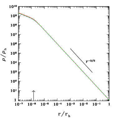
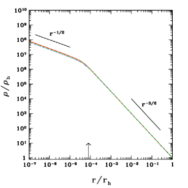
Figure 1: Fokker-Planck solution for the DM steady-state density profile $\rho(r)$ in the spike around a massive black hole, allowing for background stars. The DM distribution function cuts off at $r_{cut}=r_{mb}$ (upper figure) and $r_{ann}$ (lower figure); vertical arrows show the location of $r_{cut}$. Three stellar density profiles $\rho_{*}\sim r^{-\beta}$ are chosen for each figure: $\beta=$1 (solid, red); 7/4 (dotted, blue); 1.4 (dashed, green). The three curves are nearly indistinguishable in the plot. The densities and radii are normalized to their values near the spike outer boundary at $r_{h}$. Parameters are chosen that characterize a spike around Sgr A* in the Galactic center (see text).

II.3 Velocity Dispersion

The DM velocity dispersion may be computed from

$$v^{2}(r)=\frac{4\pi m_{\chi}}{\rho(r)}\int_{0}^{M_{bh}/r}[2(M_{bh}/r-E)]^{3/2}f(E)dE.$$ (13)

Inserting Eq. (11) into (13) yields

$$v^{2}(r)= ~{}Q(r)\frac{1-\frac{5}{2}(\frac{r_{cut}}{r})^{3/2-s}{\hat{I}}}{1-\frac{3}{2}(\frac{r_{cut}}{r_{h}})^{3/2-s}I},\ r\geq r_{cut}$$ (14)

$$= ~{}Q(r)\frac{1-(1-\frac{r}{r_{cut}})^{5/2}-\frac{5}{2}(\frac{r_{cut}}{r})^{3/2-s}{\hat{\cal I}}}{1-\frac{3}{2}(\frac{r_{cut}}{r_{h}})^{3/2-s}I},\ r<r_{cut}$$

where

$$Q(r)=\frac{6}{5}\left(\frac{M_{bh}}{r}\right)\frac{\rho_{h}r_{h}^{3/2}}{\rho(r)r^{3/2}}.$$ (15)

Appearing in the above equations are the two quantities ${\hat{I}}=\int_{0}^{1}dx(1-x)^{3/2}x^{3/2-s}=B(5/2-s,5/2)$ and also ${\hat{\cal I}}=\int_{0}^{r/r_{cut}}dx(1-x)^{3/2}x^{3/2-s}=B(r/r_{cut};5/2-s,5/2)$.

We evaluate the velocity profile given by Eq. (14) for the cases shown in Fig. 1 and plot the results in Fig. 2. Once again the profiles do not depend at all on the magnitude of the background stellar density and only insignificantly on the profile power-law $s$. As is seen most clearly in the cases for which $r_{cut}=r_{ann}$, the DM velocity dispersion profile has two distinct regimes. For $r\gg r_{cut}$ the profile is given by $v^{2}/(M_{bh}/r)=3/(p+5/2)=6/5$, as expected for a DM distribution function of the form $f(E)\sim E^{p}$ where $p=0$, or $\rho\sim r^{-3/2}$. For $r\ll r_{cut}$ the profile asymptotes to $v^{2}/(M_{bh}/r)=2$, corresponding to $p=-1$, or $\rho\sim r^{-1/2}$; this result follows from the fact that this region is filled by $E\approx 0$ particles in highly eccentric orbits near pericenter.

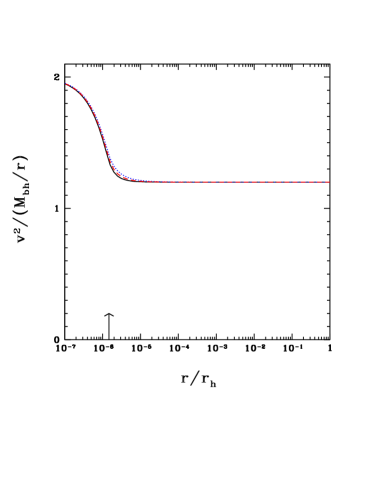
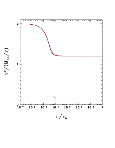
Figure 2: Fokker-Planck solution for the DM steady-state velocity dispersion profile in the spike around a massive black hole, allowing for background stars. Results are plotted for the cases shown in Fig 1 and the labelling is the same as in that figure. The velocity dispersion is normalized to the square of the local circular velocity $M_{bh}/r$.

II.4 Flux

To evaluate Eq. (7) for the constant, nonzero DM flux $\cal F$ we must first determine $K$, defined in Eq. (2). This quantity serves to normalize the stellar distribution function $f_{*}$ to yield a specifed stellar density $\rho_{*h}$ at a fiducial radius, $r_{h}$. Employing an expression identical to Eq. (II.1), but for stars rather than DM particles, yields

$$K=\frac{\rho_{*h}}{4\pi 2^{1/2}m_{*}(M_{bh}/r_{h})^{s+3/2}{\tilde{I}}}$$ (16)

where $\rho_{*h}$ is the stellar density at the spike boundary at $r=r_{h}$ and ${\tilde{I}}=\int_{0}^{1}dx(1-x)^{1/2}x^{s}=B(1+s,3/2)$. Relating $F$ to $\rho_{h}$ and $E_{cut}$ as described below Eq. (II.1) and inserting the result together with Eq. (16) into Eq. (7) yields the DM mass flux,

$${\dot{M}}=-m_{\chi}{\cal F}=C_{\cal F}\frac{\ln{\Lambda}m_{*}{\rho_{*h}}{\rho_{h}}r_{h}^{3}}{(M_{bh}/r_{h})^{3/2}},$$ (17)

where

$$C_{\cal F}=\frac{(3/2-s)3\pi^{3}}{(s+1)(s-1/2)2^{3/2}{\tilde{I}}}\frac{(r_{cut}/r_{h})^{3/2-s}}{[1-3/2(r_{cut}/r_{h}r)^{3/2-s}I]},$$ (18)

and where ${\tilde{I}}=\int_{0}^{1}dx(1-x)^{1/2}x^{s}=B(1+s,3/2)$. Using the local heating time for DM particles due to gravitational encounters with stars Merritt (2004) ($\sim$ stellar relaxation time for distant, two-body encounters, assuming comparable stellar and DM velocity dispersions ),

$$t_{r}=\frac{0.0814v^{3}}{m_{*}{\rho_{*}}\ln{\Lambda}},$$ (19)

allows us to recast Eq. (17) as

$${\dot{M}}\sim\frac{M_{DM}}{t_{rh}}\left(\frac{r_{cut}}{r_{h}}\right)^{3/2-s}\ll\frac{M_{DM}}{t_{rh}},$$ (20)

where $M_{DM}\sim 4\pi r_{h}^{3}\rho_{h}/3$ is the total DM mass inside the spike and $t_{rh}$ is the relaxation time at $r=r_{h}$.

The mass flux given in Eq. (20) is reminescent of the BW solution for the steady-state mass flux for stars onto a central black hole. BW also assumed that the distribution function was of the form $f(E,t)$, representing an isotropic system. The flux at late times was found to asymptote to the steady-state value BWf

$${\dot{M}^{*}_{BW}}\sim\frac{M_{*}}{t_{rh}}\left(\frac{r_{cut}}{r_{h}}\right)^{3/2-2s}\ll\frac{M_{*}}{t_{rh}},$$ (21)

with $M_{*}\sim 4\pi r_{h}^{3}\rho_{*h}/3$ and $s=1/4$. The difference between the exponent $s$ in Eq. (20) for the DM flux and $2s$ in Eq. (21) for the stellar flux is due to the fact that the flux of DM is driven by interactions with background stars while the flux of stars is driven by self-interactions with other stars.

A key point to appreciate is that Eqs. (20) and  (21) are both wrong! When proper allowance is made for an anisotropic velocity dispersion described by a distribution function of the form $f(E,J)$, where $J$ is the angular momentum per unit mass, it turns out that the correct flux is much larger,

$${\dot{M}_{lc}}\sim\frac{M_{h}}{t_{rh}},\ \ \ f=f(E,J)\neq f(E),$$ (22)

where $M_{h}=M_{DM}$, or $M_{h}=M_{*}$, depending on the component. The reason is that the bulk of the flux originates from high-eccentricity orbits in the outer cusp that are scattered into the black hole loss-cone and captured in an orbital period. While the loss-cone only breaks isotropy logarithmically, it significantly increases the capture rate. This result was first shown analytically in Frank and Rees (1976); Lightman and Shapiro (1977) and confirmed in more detail numerically in Shapiro and Marchant (1978); Cohn and Kulsrud (1978). [For an early review and references, see  Shapiro (1985)]. An extra sink term that roughly accounts for the DM loss-cone capture rate was inserted in the Fokker-Planck equation for $f(E,t)$ in  Merritt (2004), similar to the “patch” introduced in an earlier treatment of the equilibrium stellar distribution performed in  Lightman and Shapiro (1977) for $f(E)$ as a follow-up to the more general analysis of $f(E,J)$ in that paper. This sink term does not change the equilibrium density or velocity dispersion profile significantly. Generalizing the isotropic analysis presented here by solving instead for an anisotropic DM distribution function of the form $f(E,J)$ is possible, but not the purpose of this paper. The results should confirm those anticipated above with regard to the role of the loss-cone. Most importantly, while the flux would be significantly increased by allowing for the associated anisotropy, the modification of the density and velocity profiles would not be significant, as the deviation in $f$ from isotropy would only consist of a slowly-varying logarithmic function of $J$ that reduces the DM distribution as one approaches the loss cone at low-$J$ Frank and Rees (1976); Lightman and Shapiro (1977).

For the Galactic center we consider stars at $r_{h}$ with $\rho_{*h}=1.2\times 10^{6}~{}M_{\odot}{\rm pc}^{-3}$, $m_{*}=M_{\odot}$ and $\Lambda=0.4N,N\approx 6\times 10^{6}$ Merritt (2004). Together with the adopted parameters for the DM listed above, we then have $t_{rh}\approx 1.5\times 10^{9}~{}$yrs and a DM mass inside $r_{h}$ of $M_{DM}\approx 80~{}M_{\odot}$, which gives an anticipated DM accretion rate from Eq. (22) of $\dot{M}\sim 5\times 10^{-8}~{}M_{\odot}{\rm yr}^{-1}$.

III Two-Component Fluid Treatment

Adapting the two-component fluid formalism presented in  Bettwieser and Inagaki (1985); Heggie and Aarseth (1992) to the problem at hand, the fluid equations for the DM particles analogous to Eq. (1) become

$$\frac{\partial\rho}{\partial t}+\frac{1}{r^{2}}\frac{\partial(\rho ur^{2})}{\partial r}=0,$$ (23)

$$\frac{\partial u}{\partial t}+u\frac{\partial u}{\partial r}=\\ -\frac{1}{\rho}\frac{\partial P}{\partial r}-\frac{M_{bh}}{r^{2}},$$ (24)

$$4\pi r^{2}\rho\hat{v}^{2}\left(\frac{D}{Dt}\right)\ln\left(\frac{\hat{v}^{3}}{\rho}\right)=4\pi r^{2}\Gamma\equiv$$ (25)

$$16\pi r^{2}(2\pi)^{1/2}\ln\Lambda\left[\frac{\rho\rho_{*}}{(\hat{v}^{2}+\hat{v}_{*}^{2})^{3/2}}\right](m_{*}\hat{v}_{*}^{2}-m_{\chi}\hat{v}^{2}).$$

In the above equations, $u$ is the mean radial velocity and the pressure $P=\rho\hat{v}^{2}$, where $\hat{v}$ is the one-dimensional (i.e., line-of-sight) velocity dispersion. The dispersion is again assumed isotropic, whereby $\hat{v}^{2}=v^{2}/3$, and similarly for the stars (i.e. $\hat{v}_{*}^{2}=v_{*}^{2}/3$). The Lagrangian time derivative $D/Dt$ my be expanded in the usual way according to $D/Dt=\partial/\partial t+u\partial/\partial r$. The quantity $\Gamma$ appearing in Eq. (25) gives the DM heating rate per unit volume by gravitational scattering off stars Spitzer, Jr. (1987). The other variables appearing above have their same meanings as in Section II. Once again we assume that the background stellar profile is fixed and given by a power-law with $\rho_{*}\sim r^{-\beta}$.

The equation of state is a $\gamma$-law with $\gamma=5/3$, as it can be written in the form $P=(\gamma-1)\rho\epsilon$, where $\epsilon=3\hat{v}^{2}/2$ is the particle energy per unit mass. This identification is usually of no significance for applications involving nonrelativistic particles, such as stars in Newtonian stellar dynamics, but it will be useful below in drawing an analogy with the theory of Bondi accretion.

We note that $\Gamma$ has been derived assuming local Maxwellian velocity distributions for both components. The basic functional dependence of this term on the local density and velocity dispersion should be the same for other velocity distributions even though the numerical coeffients may change. This fact should be sufficient to give the correct scaling of the $\rho$ and $v$ profiles with $r$ even for non-Maxwellian distributions, as found in previous dynamical studies (see, e.g.,Lightman and Shapiro (1977); Young (1977)).

We are interested in solving the above fluid equations for steady-state, hence we can drop all terms involving $\partial/\partial t$. In addition, we can drop the term on the right-hand side of Eq. (25) involving $m_{\chi}$, as $m_{\chi}\hat{v}^{2}\ll m_{*}\hat{v}_{*}^{2}$. The resulting equations then become

$$4\pi r^{2}\rho u={\dot{M}}={\rm constant},$$ (26)

$$u\frac{du}{dr}=-\frac{1}{\rho}\frac{\partial P}{\partial r}-\frac{M_{bh}}{r^{2}},$$ (27)

$$-\frac{d\ln(\hat{v}^{3}/\rho)}{d\ln r}=\frac{4\pi\Gamma r^{3}}{{\dot{M}}\hat{v}^{2}}=\frac{3}{2}{\cal R},$$ (28)

where

$${\cal R} \equiv (\Gamma\frac{4}{3}\pi r^{3})/(\frac{1}{2}{\dot{M}}\hat{v}^{2})$$

$$\approx \frac{\rm heating\ rate\ inside\ r\ by\ stars}{\rm\ heat\ per\ unit\ time\ transported\ across\ r}.$$

Note that in Eq. (26) and below we take $u$ to be the magnitude of the (inward) radial velocity. In obtaining Eq. (28) we substituted Eq. (26) into Eq. (25). If everywhere ${\cal R}\ll$ 1 then the heating of DM by gravitational scattering off stars is unimportant and the DM gas is adiabatic (specific entropy $s\propto\ln(\hat{v}^{3}/\rho)=$ constant) and reduces to adiabatic Bondi flow Bondi (1952) for $\gamma=5/3$.

We solve equations (26-28) numerically without approximation in Section IIIB. In the next section we introduce a few simplificatins that enable us to solve them analytically to gain some preliminary insight.

III.1 Approximate Analytic Solution

We anticipate that the mean flow will be highly subsonic ($u\ll a$, where $a=\sqrt{\gamma P/\rho}$ is the DM sound speed), whereby we can eliminate the advective term on the left-hand side of the momentum equation (27). With this simplification (27) reduces to the equation of hydrostatic equilibrium,

$$\frac{dP}{dr}=-\frac{M_{bh}}{r^{2}}\rho.$$ (30)

Next, if we neglect heating (${\cal R}=0$) and seek power-law solutions, Eqs. (28) and (30) give

$$\rho=\rho_{h}(r_{h}/r)^{3/2},{\hat{v}}^{2}={\hat{v}_{h}}^{2}(r_{h}/r).$$ (31)

Similarly, the assumed stellar density distribution gives the corresponding expressions

$$\rho_{*}=\rho_{*h}(r_{h}/r)^{\beta},v_{*}^{2}=v_{*h}^{2}(r_{h}/r).$$ (32)

Now we treat the heating as a small perturbation on these exact expressions. For this purpose we can substitute Eqs. (31) and (32) into the perturbation term on the right of Eq. (28), finding

$${\cal R}={\cal R}_{h}(r/r_{h})^{3-\beta},$$ (33)

where ${{\cal R}}_{h}={{\cal R}}(r_{h})$. Now the perturbations to the results in Eq. (31) can be found. Details are given in Appendix A, and lead to the result that

$$\frac{\rho}{\rho_{h}} =\left(\frac{r_{h}}{r}\right)^{3/2}\Bigg{(}1+\frac{3}{10(3-\beta)(2-\beta)}{\cal R}_{h}\bigg{[}(1-2\beta)\left(\frac{r}{r_{h}}\right)^{3-\beta}$$

$$+3\left(3-\beta\right)\left(\frac{r}{r_{h}}\right)-5\left(2-\beta\right)\bigg{]}\Bigg{)}.$$ (34)

A similar expression can be easily given for the velocity dispersion.

We see from Eq. (III.1) for plausible stellar density profiles with $\beta<3$ that deep inside the cusp where $r/r_{h}\ll 1$ the DM density is approximately

$$\frac{\rho}{\rho_{h}}=\left(\frac{r_{h}}{r}\right)^{3/2}\Bigg{(}1-\frac{3{\cal R}_{h}}{2(3-\beta)}\Bigg{)},$$ (35)

i.e. it assumes the same power-law profile $\rho\sim r^{-3/2}$ that we found in the Fokker-Planck analysis away from the inner boundary at $r=r_{cut}$ (see Eq. (12)). By Eq. (30) we also get the same velocity dispersion deep inside the cusp, $v^{2}=3\hat{v}^{2}=(6/5)M_{bh}/r$ (see Eqs. (14) and (15)). We also find, using Eq. (33), that in the cusp the solution asymptotes to the adiabatic Bondi solution as $r$ decreases, and is adiabatic everywhere if ${{\cal R}}_{h}\ll 1$.

In our Fokker-Planck treatment it was possible to choose the flux in energy space to make $f(E_{cut})=0$. In the two-fluid approach it is tempting to adjust the mass-flux (or, equivalently, ${\cal R}_{h}$) to make $\rho(r_{cut})=0$. While Eq. (35) shows that $\rho(r)$ at fixed $r$ decreases as ${\cal R}_{h}$ increases, it cannot be shown to make $\rho$ vanish within the perturbation theory, which assumes that ${\cal R}_{h}$ is small. But even if we were able to solve the present fluid equations without approximation, such a boundary condition would be problematic: requiring $\rho(r_{cut})=0$ with a non-zero mass flux contradicts our assumption that the flow is very subsonic.

To summarise at this point: we note that the two-fluid approach, in contrast to our Fokker-Planck treatment, does not yield a unique value for the DM mass accretion rate, $\dot{M}$. This fact is reminiscent of steady-state, adiabatic Bondi flow, for which $\dot{M}$ is a free parameter that yields viable accretion solutions for all values up to a maximum, ${\dot{M}}_{max}$, that depends on $\gamma$. We will return to this issue in the next section, once we have solved the fluid equations without simplifying approximations.

Before proceeding, however, we make one further observation. One way to impose a reduction in the fluid density at $r_{cut}$, having imposed boundary conditions at $r_{h}$, would be to add a sink term on the right-hand side of Eq. (23) to effectively cut down the DM density inside $r_{cut}$. While the DM density and flux are not reduced at $r_{mb}$ when DM is treated as a fluid, they can be reduced by annihilations. Hence one could introduce a collision term on the right-hand side to account for annihilations that would become important inside $r\lesssim r_{ann}$, or even a sink term to model the effect of the loss cone, analogous to that introduced in the isotropic Fokker-Planck equation in Lightman and Shapiro (1977); Merritt (2004). However, implementing these modifications is beyond the scope of this paper, and we shall leave it for a future investigation.

III.2 Exact Numerical Solution

The basic fluid equations (26)-(28) are recognized as the usual steady-state, spherical Bondi flow equations with a heating term on the right-hand side of (28). We recently have worked with a similar set of equations, but in a different context Bennewitz et al. (2019), namely the accretion of baryonic gas accreting onto a SMBH (e.g. Sgr A*) heated by DM annihilation. Adapting that “heated Bondi accretion” formalism to the problem at hand, we can recast the nonadiabatic fluid equations as follows:

$$\frac{dK_{D}}{dr} = -\frac{(\gamma-1)\Gamma}{\rho^{\gamma}u},$$ (36)

$$\frac{d\rho}{dr} = -\rho\frac{D_{2}+H}{D},$$ (37)

$$u = \frac{\dot{M}}{4\pi\rho r^{2}},$$ (38)

where

$$D_{2} = \frac{2u^{2}}{r}-\frac{M_{bh}}{r^{2}},$$ (39)

$$D = u^{2}-a^{2},$$ (40)

$$H = \frac{(\gamma-1)\Gamma}{\rho u},$$ (41)

and where $a$ is the sound speed, $P=\rho\hat{v}^{2}=K_{D}\rho^{\gamma}$, $\gamma=5/3$, and $\Gamma$ is again given by Eq. (25).

In the absence of heating, $\Gamma=0$, $K_{D}=$ constant, and the solution reduces to steady-state, adiabatic Bondi flow onto a point mass $M_{bh}$ for $\gamma=5/3$. In this case ${\dot{M}}$ is an eigenvalue which yields valid solutions for all values in the range $0\leq{\dot{M}}\leq{\dot{M}}_{max}$, where

$${\dot{M}}_{max}=4\pi\rho_{h}u_{h}r_{h}^{2}=4\pi\lambda M_{bh}^{2}\rho_{\infty}a_{\infty}^{-3},\ \ \ \lambda=1/4.$$ (42)

and where the second equality assumes that the fluid is at rest and homogeneous at infinity. The solution with ${\dot{M}}={\dot{M}}_{max}$ is the only one with $\gamma=5/3$ that passes through a critical transonic point, at which $u=a$. This point is only reached at $r=0$, while for all $r>0$ the flow remains subsonic. For all other ${\dot{M}}<{\dot{M}}_{max}$ the flow is subsonic everywhere.

As described above, the Newtonian, adiabatic, steady-state Bondi equations do not determine ${\dot{M}}$ uniquely. However, the general relativistic analogue of these equations for spherical flow onto a Schwarzshild black hole shows that the flow must pass through a critical point to preserve the causality constraint $a^{2}<1$ and hence this constraint singles out flow with $\dot{M}={\dot{M}}_{max}$ as the unique solution for steady-state flow Shapiro and Teukolsky (1983). Furthermore, typical time-dependent integrations for adiabatic, spherical accretion (i.e. Eqs. (23)-(25) with $\Gamma=0$) settle on ${\dot{M}}={\dot{M}}_{max}$ when allowed to reach steady-state, even in the Newtonian case.

We have integrated Eqs. (36)-(37) inward numerically from $r=r_{h}$, adopting the same physical values used in Section IIB in our Fokker-Planck treatment for the (outer) boundary conditions required by the ODEs for the variables $K_{h}$ and $\rho_{h}$ that we set at $r=r_{h}$. We set $\beta=1.4$ for the background stellar density profile, $\rho_{*}\sim r^{-\beta}$ and $v_{h}=v_{0}=v_{*h}$.

III.2.1 Flux

We have considered four cases for the mass accretion rate $\dot{M}$, which, as in the case for adiabatic Bondi flow, is not determined uniquely in steady-state. In particular, we treat

$${\dot{M}}=q\frac{M_{DM}}{t_{rh}}$$ (43)

where $t_{r}$ is defined in Eq. (19), $M_{DM}$ is defined just below Eq. (20) and where we considered four values of $q$ in the range $0.1\leq q\leq 100$. The chosen range for $\dot{M}$ was motivated by the (unique) value expected from a fundamental Fokker-Planck treatment of the problem that solves for $f(E,J)$, as discussed in Section IID (see Eq. (22)).

Comparison of Eq. (42) and (43) shows that

$$\frac{\dot{M}}{\dot{M}_{max}}\sim q\frac{t_{dynh}}{t_{rh}},$$ (44)

where $t_{dynh}=r_{h}/v_{h}$ is defined as the dynamical (crossing) timescale at $r_{h}$. Evaluating $\dot{M}_{max}$ here and below we set $a_{\infty}\sim a_{h}$ and $\rho_{\infty}\sim\rho_{h}$, as in the Bondi solution. The computed values for the adopted Galactic parameters (Sec.IIB) are $t_{dynh}\sim 2.8\times 10^{3}~{}$yrs, $t_{dynh}/t_{rh}\sim 2\times 10^{-6}$ and ${\dot{M}}/{\dot{M}_{max}}\sim q\times 1.1\times 10^{-6}$. Thus the anticipated Fokker-Planck accretion rate for which $q\sim 1$ is six orders of magnitude smaller than the likely maximum fluid rate.

III.2.2 Density

Results for the DM density profile are plotted in Fig. 3 for all four cases. The density satisfies $\rho\sim r^{-3/2}$ for $r\ll r_{h}$ in all cases. Moreover, for high values of $q$ and $\dot{M}$ the profile obeys this power-law for almost all $r$. This result is not surprising, since Fig. 4 shows that the nondimensional heating ratio ${\cal R}\sim r^{(3-\beta)}\ll 1$ for $r\ll r_{h}$ in all cases. Since ${\cal R}_{h}=3.0/q$, for sufficiently high $q\gg 1$, and thus high $\dot{M}$, the ratio is small everywhere, even at $r=r_{h}$. In the latter case the flow is essentially adiabatic and reduces to the standard adiabatic Bondi solution for $\gamma=5/3$. Our approximate analytic profile  (III.1) reproduces this behavior in the perturbative regime.

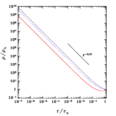
Figure 3: Two-component fluid solution for the DM steady-state density profile $\rho(r)$ in the spike around a massive black hole, allowing for background stars. The stellar density is given by $\rho_{*}\sim r^{-\beta}$, with $\beta=1.4$. Four accretion rates are chosen according to Eq. (43), with $q=$0.1 (solid, red); 1 (dotted, blue); 10 (dashed, green); 100 (dot-dashed, magenta). The densities and radii are normalized to their values at the spike outer boundary at $r_{h}$. Parameters are chosen that characterize a spike around Sgr A* in the Galactic center (see text).

Figure 4: Two-component fluid solution for the DM steady-state dimensionless heating parameter ${\cal R}(r)$ in the spike around a massive black hole, allowing for background stars (see Eq. (III)). Results are plotted for the cases shown in Fig. 3 and the labelling is the same as in that figure.

III.2.3 Velocity Dispersion

The DM velocity dispersion is plotted in Fig. 5 for the cases shown in Fig. 3. As expected (Sec.IIC), well inside the outer boundary we find $v^{2}/(M_{bh}/r)\approx 6/5$. Near $r_{h}$ the role of heating is reflected in the higher values of $v^{2}$ for cases with lower accretion rates. As the accretion rate is chosen smaller and the corresponding ratio $\cal R$ increases well above unity, the higher heating rate may subsequently unbind the outer regions of the cusp altogether. These solutions may then be unstable and a time-dependent integration of the equations might then drive the flow to smaller accretion values before settling into steady-state.

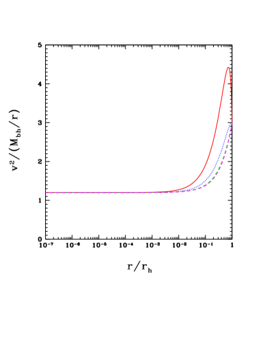
Figure 5: Two-component fluid solution for the DM steady-state velocity dispersion profile $v(r)$ in the spike around a massive black hole, allowing for background stars. Results are plotted for the cases shown in Fig. 3 and the labelling is the same as in that figure. The velocity dispersion is normalized to the square of the local circular velocity $M_{bh}/r$.

III.2.4 Mean Flow Velocity

All of our solutions are highly subsonic, as shown in Fig. 6. This behavior is expected since even in adiabatic Bondi flow when $\gamma=5/3$, the mean inflow velocity is everywhere subsonic, except when ${\dot{M}}={\dot{M}}_{max}$, in which case $u/a$ reaches unity, but only at the origin. As shown in Fig. 6, the lower the rate of accretion and the higher the corresponding value of ${\cal R}$, the more important heating becomes and the lower the Mach number $u/a$. Here $a/v=(\gamma/3)^{1/2}\approx 0.745$ while for $r\ll r_{h}$ we have $u/a\sim{\rm few}\times q(t_{dynh}/t_{rh})\sim{\rm few}\times 10^{-6}q$, which is roughly consistent with Fig. 6.

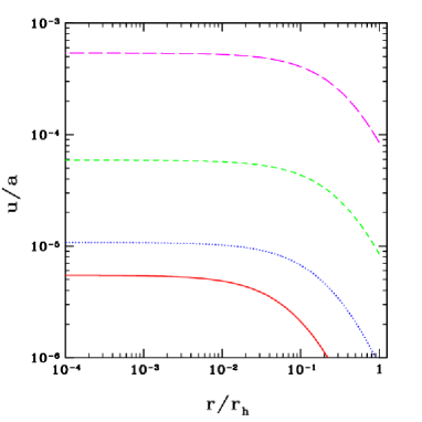
Figure 6: Two-component fluid solution for the DM steady-state Mach number $u(r)/a(r)$ in the spike around a massive black hole, allowing for background stars. Results are plotted for the cases shown in Fig. 3 and the labelling is the same as in that figure.

IV Discussion

Spherical accretion onto a BH by collisionless matter undergoing repeated, small-angle, gravitational scattering is qualitatively different from accretion of fluid matter. In the former case most of the captured particles move on highly eccentric orbits that have apocenters far from the central hole and are scattered into a loss-cone and captured in one period. In the latter case, the captured gas moves radially as a continuous fluid, becoming tightly bound to the black hole before plunging in. All nonradial motion is damped in the case of spherical fluid flow  Shapiro and Teukolsky (1983). Not surprisingly, the accretion rates calculated by treating DM by these two different descriptions result in two different answers.

The steady-state rate of accretion anticipated from a Fokker-Planck treatment of $f(E,J)$, i.e. Eq. (43) with $q\sim 1$, is orders of magnitude less than $\dot{M}_{max}$ for adiabatic Bondi flow given by Eq. (42). The simple flux ratio given by Eq. (44) highlights this fact. Yet heating is likely to be unimportant (${\cal R}\ll 1$) well inside the spike. Hence we anticipate that as the flow approaches the BH, a general relativistic treatment will likely pick out $\dot{M}_{max}$ as the steady-state solution, just as it does for the equations describing adiabatic Bondi flow, to which the DM fluid equations reduce deep inside the spike and near the black hole. Even a time-dependent Newtonian integration of the equations is likely to relax to this solution. However, this difference in the predicted accretion rate should not lead to a major discrepancy in the computed DM density or velocity dispersion profiles. We have already seen that we obtain the same basic power-law profiles well inside the spike when comparing the two-fluid solution to the Fokker Planck profiles associated with an isotropic $f(E)$. Similar agreement is expected when we compare with the profiles assciated with an anisotropic $f(E,J)$, up to slowly varying logarithmic factors, as was proven to be the case for stars in a BW cusp around a BH.

The agreement between Fokker-Planck and fluid profiles breaks down only near the outer boundary whenever we have $R_{h}\gtrsim 1$, as well as near the inner boundary, since there additional conditions can be imposed as inner boundary conditions in the Fokker-Planck solution to constrain the distribution function. Constraining the fluid profile similarly requires the addition of sink terms in the continuity equation, a departure from the standard two-fluid equations.

Generalizing from this and earlier analyses (e.g. Bettwieser and Inagaki (1985); Heggie and Aarseth (1992); Spurzem and Takahashi (1995)), of multi-component, large $N$-body dynamical systems undergoing secular evolution on relaxation timescales due to gravitational scattering, we infer that the multi-component fluid approach yields similar results to a fundamental Fokker-Planck treatment in many important aspects, but not all, depending on the system. One must bear this in mind when adopting what is often a computationally simpler fluid description to describe such a system.

Acknowledgments: It is a pleasure to thank R. Spurzem for useful discussions. This paper was supported in part by NSF Grant PHY-2006066 and NASA Grant 80NSSC17K0070 to the University of Illinois at Urbana-Champaign.

Appendix A Solution of perturbed fluid equations

The purpose of this appendix is to derive Eq. (III.1) for the density in the case of weak heating. The equations to be solved are Eqs. (28) and (30), and the right side of the former represents heating. We regard this term as a perturbation of the no-heating exact solutions of Eq. (31), which we denote by $\rho_{0}$, $\hat{v}_{0}$, respectively. Thus we write the perturbed solution as $\rho=\rho_{0}(1+f),\hat{v}=\hat{v}_{0}(1+g)$, where $f,g$ are functions of order ${\cal R}$. Substituting into Eq. (28), and retaining terms only up to first order in ${\cal R}$, we have

$$-\frac{d}{d\ln r}\left(\ln\left(\frac{\hat{v}_{0}^{3}}{\rho_{0}}\right)+3g-f\right)=\frac{3}{2}{\cal R}.$$ (45)

The 0-order term vanishes, as the functions $\rho_{0},\hat{v}_{0}$ solve the unheated equation exactly, which leads to

$$-r(3g^{\prime}-f^{\prime})=(3/2){\cal R}_{h}(r/r_{h})^{3-\beta},$$ (46)

where we have used Eq. (III), and a prime denotes an $r$-derivative. This integrates to

$$3g-f=-\frac{3{\cal R}_{h}}{2(3-\beta)}\left(\frac{r}{r_{h}}\right)^{3-\beta}+C,$$ (47)

where $C$ is a constant of integration.

In much the same way, Eq. (30) gives

$$f+2g+\frac{\rho_{0}\hat{v}_{0}^{2}}{\left(\rho_{0}\hat{v}_{0}^{2}\right)^{\prime}}(f^{\prime}+2g^{\prime})=f,$$ (48)

and so, by Eq. (31),

$$-\frac{5}{r}g+f^{\prime}+2g^{\prime}=0.$$ (49)

Next, Eqs. (46) and (47) let us remove $g$ and $g^{\prime}$ from Eq. (49), whence

$$f^{\prime}-\frac{f}{r}=\frac{3(1-2\beta)}{10(3-\beta)}\frac{{\cal R}_{h}}{r_{h}}\left(\frac{r}{r_{h}}\right)^{2-\beta}+\frac{C}{r}.$$ (50)

By trying power-law solutions $f\propto r^{\lambda}$ for $\lambda=3-\beta,0$ and $1$ and superposing, we obtain the general solution

$$f=\frac{3}{10}\frac{1-2\beta}{(3-\beta)(2-\beta)}{\cal R}_{h}\left(\frac{r}{r_{h}}\right)^{3-\beta}-C+Dr,$$ (51)

where $D$ is another constant. The two constants $C$ and $D$ can be chosen so that both $f$ and $g$ vanish at $r=r_{h}$, which yields

$$C=\frac{3}{2(3-\beta)}{{\cal R}_{h}},\ \ \ D=\frac{6(2+\beta)}{10(3-\beta)}\frac{{\cal R}_{h}}{r_{h}},$$ (52)

obtaining Eq. (III.1).

References

- Navarro et al. (1997) J. F. Navarro, C. S. Frenk, and S. D. M. White, Astrophys. J. 490, 493 (1997).
- Diemand et al. (2008) J. Diemand, M. Kuhlen, P. Madau, M. Zemp, B. Moore, D. Potter, and J. Stadel, Nature (London) 454, 735 (2008).
- Navarro et al. (2010) J. F. Navarro, A. Ludlow, V. Springel, J. Wang, M. Vogelsberger, S. D. M. White, A. Jenkins, C. S. Frenk, and A. Helmi, Mon. Not. R. Astro. Soc. 402, 21 (2010).
- Blumenthal et al. (1986) G. R. Blumenthal, S. M. Faber, R. Flores, and J. R. Primack, Astrophys. J. 301, 27 (1986).
- Gnedin et al. (2004) O. Y. Gnedin, A. V. Kravtsov, A. A. Klypin, and D. Nagai, Astrophys. J. 616, 16 (2004).
- Gustafsson et al. (2006) M. Gustafsson, M. Fairbairn, and J. Sommer-Larsen, Phys. Rev. D 74, 123522 (2006).
- Pato et al. (2015) M. Pato, F. Iocco, and G. Bertone, JCAP 12, 001 (2015).
- Peebles (1972) P. J. E. Peebles, General Relativity and Gravitation 3, 63 (1972).
- Gondolo and Silk (1999) P. Gondolo and J. Silk, Physical Review Letters 83, 1719 (1999).
- Merritt (2004) D. Merritt, Physical Review Letters 92, 201304 (2004).
- Gnedin and Primack (2004) O. Y. Gnedin and J. R. Primack, Physical Review Letters 93, 061302 (2004).
- Merritt et al. (2007) D. Merritt, S. Harfst, and G. Bertone, Phys. Rev. D 75, 043517 (2007).
- Wanders et al. (2015) M. Wanders, G. Bertone, M. Volonteri, and C. Weniger, JCAP 4, 004 (2015).
- Begelman et al. (2006) M. C. Begelman, M. Volonteri, and M. J. Rees, Mon. Not. R. Astro. Soc. 370, 289 (2006).
- Ullio et al. (2001) P. Ullio, H. Zhao, and M. Kamionkowski, Phys. Rev. D 64, 043504 (2001).
- Fornasa and Bertone (2008) M. Fornasa and G. Bertone, Inter. J. Mod. Phys. D 17, 1125 (2008).
- Shapiro and Paschalidis (2014) S. L. Shapiro and V. Paschalidis, Phys. Rev. D 89, 023506 (2014).
- Feng et al. (2021) W.-X. Feng, H.-B. Yu, and Y.-M. Zhong, Astrophys. J. Lett. 914, L26 (2021).
- El-Zant et al. (2001) A. El-Zant, I. Shlosman, and Y. Hoffman, Astrophys. J. 560, 636 (2001).
- Romano-Díaz et al. (2008) E. Romano-Díaz, I. Shlosman, Y. Hoffman, and C. Heller, Astrophys. J. Lett. 685, L105 (2008).
- Vasiliev (2007) E. Vasiliev, Phys. Rev. D 76, 103532 (2007).
- Shapiro and Shelton (2016) S. L. Shapiro and J. Shelton, Phys. Rev. D 93, 123510 (2016).
- Gonzalez-Morales et al. (2014) A. X. Gonzalez-Morales, S. Profumo, and F. S. Queiroz, Phys. Rev. D 90, 103508 (2014).
- Fields et al. (2014) B. D. Fields, S. L. Shapiro, and J. Shelton, Physical Review Letters 113, 151302 (2014).
- Belikov and Silk (2014) A. Belikov and J. Silk, Phys. Rev. D 89, 043520 (2014).
- Lacroix et al. (2015) T. Lacroix, C. Boehm, and J. Silk, Phys. Rev. D 92, 043510 (2015).
- Shelton et al. (2015) J. Shelton, S. L. Shapiro, and B. D. Fields, Physical Review Letters 115, 231302 (2015).
- Daylan et al. (2016) T. Daylan, D. P. Finkbeiner, D. Hooper, T. Linden, S. K. N. Portillo, N. L. Rodd, and T. R. Slatyer, Physics of the Dark Universe 12, 1 (2016).
- Calore et al. (2015) F. Calore, I. Cholis, and C. Weniger, JCAP 1503, 038 (2015).
- Ajello (2016) M. Ajello, et al. (Fermi-LAT collaboration) Astrophys. J. 819, 44 (2016).
- Ackermann (2015) M. Ackermann, et al. (Fermi-LAT collaboration) Phys. Rev. Lett. 115, 231301 (2015).
- Lee et al. (2016) S. K. Lee, M. Lisanti, B. R. Safdi, T. R. Slatyer, and W. Xue, Phys. Rev. Lett. 116, 051103 (2016).
- Bartels et al. (2016) R. Bartels, S. Krishnamurthy, and C. Weniger, Phys. Rev. Lett. 116, 051102 (2016).
- Abazajian et al. (2014) K. N. Abazajian, N. Canac, S. Horiuchi, and M. Kaplinghat, Phys. Rev. D 90, 023526 (2014).
- Brandt and Kocsis (2015) T. D. Brandt and B. Kocsis, Astrophys. J. 812, 15 (2015).
- O’Leary et al. (2016) R. M. O’Leary, M. D. Kistler, M. Kerr, and J. Dexter (2016), eprint 1601.05797.
- Bettwieser and Inagaki (1985) E. Bettwieser and S. Inagaki, Mon. Not. R. Astro. Soc. 213, 473 (1985).
- Heggie and Aarseth (1992) D. C. Heggie and S. J. Aarseth, Mon. Not. R. Astro. Soc. 257, 513 (1992).
- Spurzem and Takahashi (1995) R. Spurzem and K. Takahashi, Mon. Not. R. Astro. Soc. 272, 772 (1995).
- Spitzer, Jr. (1987) L. Spitzer, Jr., Dynamical Evolution of Globular Clusters (Princeton, NJ, Princeton University Press, 1987).
- Bahcall and Wolf (1976) J. N. Bahcall and R. A. Wolf, Astrophys. J. 209, 214 (1976).
- Frank and Rees (1976) J. Frank and M. J. Rees, Mon. Not. R. Astro. Soc. 176, 633 (1976).
- Lightman and Shapiro (1977) A. P. Lightman and S. L. Shapiro, Astrophys. J. 211, 244 (1977).
- Genzel et al. (2003) R. Genzel, R. Schodel, T. Ott, F. Eisenhauer, R. Hofmann, M. Lehnert, A. Eckart, T. Alexander, A. Sternberg, R. Lenzen, et al., The Astrophysical Journal 594, 812–832 (2003).
- Genzel et al. (2010) R. Genzel, F. Eisenhauer, and S. Gillessen, Reviews of Modern Physics 82, 3121 (2010).
- Ghez et al. (2008) A. M. Ghez, S. Salim, N. N. Weinberg, J. R. Lu, T. Do, J. K. Dunn, K. Matthews, M. R. Morris, S. Yelda, E. E. Becklin, et al., Astrophys. J. 689, 1044 (2008).
- Bovy and Tremaine (2012) J. Bovy and S. Tremaine, Astrophys. J. 756, 89 (2012).
- Gültekin et al. (2009) K. Gültekin, D. O. Richstone, K. Gebhardt, T. R. Lauer, S. Tremaine, M. C. Aller, R. Bender, A. Dressler, S. M. Faber, A. V. Filippenko, et al., Astrophys. J. 698, 198 (2009).
- (49) see, e.g., BW, Eqs. (62a) and (63), or Ref Lightman and Shapiro (1977), Eqs. (6) and (7), where the tidal disruption radius .
- Shapiro and Marchant (1978) S. L. Shapiro and A. B. Marchant, Astrophys. J. 225, 603 (1978).
- Cohn and Kulsrud (1978) H. Cohn and R. M. Kulsrud, Astrophys. J. 226, 1087 (1978).
- Shapiro (1985) S. L. Shapiro, in Dynamics of Star Clusters, edited by J. Goodman and P. Hut (1985), vol. 113 of IAU Symposium, pp. 373–412.
- Young (1977) P. J. Young, Astrophys. J. 217, 287 (1977).
- Bondi (1952) H. Bondi, Mon. Not. R. Astro. Soc. 112, 195 (1952).
- Bennewitz et al. (2019) E. R. Bennewitz, C. Gaidau, T. W. Baumgarte, and S. L. Shapiro, Mon. Not. R. Astro. Soc. 490, 3414 (2019).
- Shapiro and Teukolsky (1983) S. L. Shapiro and S. A. Teukolsky, Black Holes, White Dwarfs, and Neutron Stars: The Physics of Compact Objects (New York, Wiley, 1983).