Magnetohydrodynamic Simulations of the Tayler Instability in Rotating Stellar Interiors

Abstract

The Tayler instability is an important but poorly studied magnetohydrodynamic instability that likely operates in stellar interiors. The nonlinear saturation of the Tayler instability is poorly understood and has crucial consequences for dynamo action and angular momentum transport in radiative regions of stars. We perform three-dimensional MHD simulations of the Tayler instability in a cylindrical geometry, including strong buoyancy and Coriolis forces as appropriate for its operation in realistic rotating stars. The linear growth of the instability is characterized by a predominantly $m=1$ oscillation with growth rates roughly following analytical expectations. The non-linear saturation of the instability appears to be caused by secondary shear instabilities and is also accompanied by a morphological change in the flow. We argue, however, that non-linear saturation likely occurs via other mechanisms in real stars where the separation of scales is larger than those reached by our simulations. We also observe dynamo action via the amplification of the axisymmetric poloidal magnetic field, suggesting that Tayler instability could be important for magnetic field generation and angular momentum transport in the radiative regions of evolving stars.

1 Introduction

The interplay between rotation and magnetism is crucial for understanding the evolution of stars and the compact objects they produce. Differential rotation generated by contracting stellar cores may source various magnetohydrodynamic (MHD) instabilities that can amplify magnetic fields and/or transport AM outwards to slow the rotation of the stellar core. However, the instabilities at work and their saturation mechanisms remain poorly understood.

Asteroseismic observations have helped by providing internal rotation rate measurements for stars on the main sequence (Kurtz et al., 2014; Saio et al., 2015; Benomar et al., 2015; Van Reeth et al., 2018), sub-giant/red giant branch (RGB) (Beck et al., 2012; Mosser et al., 2012; Deheuvels et al., 2014; Triana et al., 2017; Gehan et al., 2018), red clump (Mosser et al., 2012; Deheuvels et al., 2015), and finally in WD remnants (Hermes et al., 2017). The conclusion drawn from these measurements is unambiguous: core rotation rates are relatively slow, and the vast majority of AM is extracted from stellar cores as they evolve. The spin rates of red giant cores and WDs are slower than theoretically predicted by nearly all hydrodynamic AM transport mechanisms (Fuller et al., 2014; Belkacem et al., 2015; Spada et al., 2016; Eggenberger et al., 2017; Ouazzani et al., 2019).

The non-axisymmetric MHD Tayler instability (Tayler, 1973; Spruit, 1999; Goldstein et al., 2019) is likely the most important MHD instability in radiative regions of stars. Tayler instability is a kink-type instability of toroidal (azimuthal) fields that have been created by winding up a radial seed field through differential rotation. Above a critical field strength, field loops slip sideways relative to one another with a predominantly non-axisymmetric $m=1$ wavenumber. While the dynamics of the linear instability are well understood, the nonlinear (and likely turbulent) saturation of the instability, and the resulting AM transport are poorly understood and controversial (e.g., Braithwaite, 2006; Zahn et al., 2007).

The Tayler-Spruit (TS) dynamo (Spruit, 2002) is one possible saturation mechanism of the Tayler instability. In this theory, toroidal magnetic field energy is turbulently dissipated by the fluid motions, and the instability saturates when the turbulent dissipation rate is equal to the energy input via winding of the radial field. In the presence of a composition gradient, the resulting torque density due to Maxwell stresses is

$$T_{\rm TS}\sim\rho r^{2}\Omega^{2}q^{3}\left(\frac{\Omega}{N_{\rm eff}}\right)^{4}\,,$$ (1)

where $q=d\ln\Omega/d\ln r$ is the dimensionless radial shear, and $N_{\rm eff}$ is the effective stratification, which is usually nearly equal to the compositional stratification $N_{\mu}$ in post-MS stars. The TS dynamo has been implemented into many stellar evolution codes, but it predicts much faster core rotation than observed in post-MS stars (Cantiello et al., 2014).

However, Fuller et al. (2019) argued that Spruit (2002) overestimated the energy damping rate of the instability, because only magnetic energy in the disordered (perturbed) field can be turbulently damped. By calculating an energy damping rate due to weak magnetic turbulence, Fuller et al. (2019) argued the instability can grow to larger amplitudes, producing a larger Maxwell stress in its saturated state. Fuller et al. (2019) find the Tayler torques are

$$T_{\rm TSF}=\alpha^{3}\rho r^{2}\Omega^{2}q\left(\frac{\Omega}{N_{\rm eff}}\right)^{2}\,,$$ (2)

where $\alpha$ is a saturation parameter of order unity. The different scaling is very important because $\Omega/N_{\rm eff}\sim 10^{-4}$ in RGB stars, so the prescription of Fuller et al. (2019) allows for significantly more AM transport.

Because the saturation of the Tayler instability is a complex and nonlinear process, it is important to examine this process via numerical simulations. The Tayler instability has been seen in a few simulations, but only in limited configurations not including both rotation and realistic stratification. Weber et al. (2015) and Gellert et al. (2008) used $N=0$ (i.e., no stratification) and Guerrero et al. (2019) used $\Omega=0$ (i.e., no rotation). The first simulation of the Tayler instability with shear and buoyancy (Braithwaite, 2006) was compressible, limiting the dynamic range and time scale over which simulations could be performed. Those simulations used $\Omega/N=1$, in stark contrast to the values of $\Omega/N\sim 10^{-4}\ll 1$ expected in real stars. The analytic predictions of Spruit (2002) and Fuller et al. (2019) also assume $\Omega\ll N$, so it is important to simulate that parameter regime. Recently, Petitdemange et al. (2023) presented a suite of simulations of Tayler instability, finding apparent agreement with the prediction of Eq. (1), which we discuss further in Section 4.

In this work, we perform three-dimensional MHD simulations of the Tayler instability, including both stratification and rotation. We also vary dimensionless parameters over a small range in an attempt to determine scaling relations and extrapolate the nature of the saturated state to parameters characteristic of real stars. Our paper is organized as follows. The numerical methods and selected parameters are described in §2. In §3, we discuss the results regarding the linear and non-linear evolution of the Tayler instability. We finally conclude in §4.

2 Methods & Simulation Setup

2.1 Simulation code

We use the spectral MHD code Dedalus (Burns et al., 2020) for our simulations. We use version 2.2006 of the code with commit hash 9bf7eb1. Because of its spectral nature, Dedalus can achieve comparable accuracy with relatively lower resolutions compared with extremely high-resolution simulations using finite-volume codes, and it parallelizes efficiently using MPI. This feature is particularly useful for our 3D simulations, since only in three dimensions can the Tayler instability develop. Dedalus has already demonstrated its ability to handle different types of MHD problems including effects of stratification and nearly incompressible dynamics including convection, waves, and magnetic fields (e.g., Lecoanet et al., 2015, 2017; Couston et al., 2018).

2.2 Initial conditions

For convenience, we non-dimensionalize the initial conditions by setting the characteristic scales (width $L_{\mathrm{box}}$, averaged gas density $\bar{\rho}$ and gravity $g$) to unity $1$. To mimic a latitudinal band of a star, our simulations are performed in 3D cylindrical coordinates $(r,z,\phi)$ with the domain size of

$$R_{\mathrm{in}}\leq r\leq R_{\mathrm{out}}$$ (3)

$$-Z\leq z\leq Z$$ (4)

$$0\leq\phi\leq 2\pi,$$ (5)

where $R_{\mathrm{in}}=L_{\mathrm{box}}$, $R_{\mathrm{out}}=2L_{\mathrm{box}}$ and $Z=L_{\mathrm{box}}/2$ . We set up initial conditions as a magnetized, gravitationally stratified medium with density gradient $d\rho_{0}/dz$ and gravitational acceleration $\bm{g}$ along the $z$-axis:

$$\rho_{0}(z)=\bar{\rho}+\frac{d\rho_{0}}{dz}z$$ (6)

$$\bm{g}=-g\hat{\bm{e}}_{z}\,.$$ (7)

Here, $\rho_{0}$ denotes the density of the unperturbed state which is a function of the scale height $z$. The averaged density $\bar{\rho}$, and the density gradient $d\rho_{0}/dz$ are constants.

We initialize the simulation with a toroidal magnetic field $\bm{B}$ along $\phi$-direction, with a power-law profile in radius:

$$\bm{B}(r)=B_{0}\left(\frac{r}{R_{\mathrm{in}}}\right)^{p}\hat{\bm{e}}_{\phi}\,,$$ (8)

where $B_{0}$ and $p$ are constant. Here we use $p=2$ for the initial magnetic field profile which is expected to be Tayler unstable (Tayler, 1973). The system is initially in magnetostatic equilibrium with the unperturbed pressure $p_{0}$ satisfying:

$$\frac{\partial(p_{0}+B^{2}/2)}{\partial r}=\left|(\bm{B}\cdot\nabla)\bm{B}\right|_{r}$$ (9)

$$\frac{\partial p_{0}}{\partial z}=-\rho_{0}g$$ (10)

$$\frac{\partial p_{0}}{\partial\phi}=0,$$ (11)

such that pressure gradients are balanced by magnetic forces and gravity respectively in the $r$ and $z$ directions.

2.3 Initial perturbations

Since the Tayler instability is a non-axisymmetric instability, initially non-axisymmetric perturbations are needed, otherwise, perfect axisymmetry will be maintained throughout the simulations. To maintain $\nabla\cdot\bm{B}=0$, we effectively evolve the magnetic vector potential $\bm{A}$ in our equation sets with $\bm{B}\equiv\nabla\times\bm{A}$. We initialize white-noise perturbations to the magnetic fields by setting the magnetic potential vector $\bm{A}$ as:

$$\bm{A}=10^{-10}B_{0}W[0,1]r\hat{\bm{e}}_{r}-\frac{B_{0}r^{p+1}}{(p+1)R_{\mathrm{in}}^{p}}\hat{\bm{e}}_{z},$$ (12)

where $W[0,1]$ is a random number uniformly distributed between $0$ and $1$. By taking $\bm{B}=\nabla\times\bm{A}$, we obtain divergence-free magnetic fields with $B_{\phi}$ in desired form in Eq. (8) and white noise perturbations with a magnitude of $\sim\!10^{-10}B_{0}$ in $B_{z}$ and $B_{\phi}$. Because the white noise distribution does not introduce any characteristic length scales, these initial conditions do not add to the initial magnitude of any particular modes.

2.4 Governing equations

We express fluid quantities as the sum of the unperturbed fields (denoted by the subscript $0$) and the variations (denoted by the prime symbol), e.g., $\rho=\rho_{0}+\rho^{\prime}$, $p=p_{0}+p^{\prime}$, etc., and solve the following fundamental governing equations of incompressible magnetohydrodynamics:

$$\frac{D\rho^{\prime}}{Dt}=\frac{\bar{\rho}}{g}N^{2}u_{z}+\kappa\nabla^{2}\rho^{\prime}$$ (13)

$$\frac{D\bm{u}}{Dt}=-\nabla\left(\frac{p^{\prime}}{\bar{\rho}}\right)+\frac{\rho^{\prime}}{\bar{\rho}}\bm{g}+\frac{(\nabla\times\bm{B})\times\bm{B}}{\bar{\rho}}-2\bm{\Omega_{0}}\times\bm{u}+\nu\nabla^{2}\bm{u}$$ (14)

$$\nabla\cdot\bm{u}=0$$ (15)

$$\frac{\partial{\bm{B}}}{\partial t}=\nabla\times\left(\bm{u}\times\bm{B}\right)+\eta\nabla^{2}\bm{B}$$ (16)

$$\nabla\cdot\bm{B}=0,$$ (17)

where $D/Dt$ denotes $\partial/\partial t+\bm{u}\cdot\nabla$, $\bm{u}$ is the fluid velocity, and $N$ is the Brunt-Väisälä frequency defined as:

$$N^{2}\equiv-\frac{\partial\rho_{0}}{\partial z}\frac{g}{\bar{\rho}}.$$ (18)

We use a Boussinesq approximation that $|\rho-\bar{\rho}|\ll|\bar{\rho}|$, which is acceptable because of the incompressible nature of the Tayler instability and its short radial length scale. Vertical stratification appears through the buoyancy term, which appears in spite of the Boussinesq approximation. This mimics a simulation of a star over a radial length scale much less than the density scale height. We transform our simulations into the rotating frame by adding the Coriolis term $2\bm{\Omega_{0}}\times\bm{u}$, with bulk angular velocity $\bm{\Omega}_{0}=\Omega_{0}\hat{\bm{e}}_{z}$. We include explicit diffusivity, viscosity and magnetic resistivity as $\kappa$, $\nu$ and $\eta$ respectively, where the diffusivity mimics the compositional diffusivity in a real star. Temperature perturbations are not included because the instability operates in an isothermal regime in post-MS stars. Since the magnetic diffusivity is usually larger than microscopic viscosity in real stars, we adopt a relatively large magnetic diffusivity $\eta$ with $\eta>\kappa\sim\nu$.

2.5 Boundary conditions

We apply periodic boundary conditions along the $z$ and $\phi$-directions. Note that although a density profile in the $z$ direction is implied as described by Eq. (6), what actually solved in the governing equations (13) – (17) are variations of fluid quantities (e.g., $\rho^{\prime}$, $p^{\prime}$, $\bm{u}$, $\bm{B}$, etc.), therefore periodic boundary conditions can be applied to the $z$-axis. We apply $\rho^{\prime}=0$, $p^{\prime}=0$ and $\bm{u}=0$ at the inner and outer boundaries. We apply the electric scalar potential $\phi_{E}=0$ and the magnetic potential $A_{\phi}=0$ and on both inner and outer boundaries, and $A_{z}(r=R_{\mathrm{in}})=-B_{0}(p+1)^{-1}R_{\mathrm{in}}$ and $A_{z}(r=R_{\mathrm{out}})=-B_{0}(p+1)^{-1}R_{\mathrm{out}}^{p+1}R_{\mathrm{in}}^{-p}$ at the inner and outer boundaries respectively, in order to maintain continuity in the magnetic potential described by Eq. (12). These boundary conditions are consistent with the initial field profile but allow the magnetic field to evolve. The boundary conditions enforce the toroidal magnetic flux to be conserved, but the magnetic energy can decrease (although it cannot go to zero).

2.6 Simulation parameters

	Resolution	Averaged density $\bar{\rho}$	Gravity $g$	Diffusivity $\kappa$	Viscosity $\nu$	Magnetic resistivity $\eta$
Value	$512\times 512\times 64$	$1$	$1$	$10^{-5}$	$10^{-5}$	$2\times 10^{-5}$
Note	in $r\times z\times\phi$			corresponds to the Prandtl number of $\mathrm{Pr}\equiv\frac{\nu}{\kappa}=1$ and the magnetic Prandtl number of $\mathrm{Pr_{m}}\equiv\frac{\nu}{\eta}=0.5$

	Angular frequency $\Omega_{0}$					Alfvén frequency $\omega_{\mathrm{A}}$			Brunt-Väisälä frequency $N$
Value	$0.3$	$0.4$	$0.5$	$0.6$	$0.7$	$0.2$	$0.25$	$0.3$	$0.9$	$1$	$1.3$	$1.5$
Name	Om.3	Om.4	Om.5	Om.6	Om.7	OmA.2	OmA.25	OmA.3	N.9	N1	N1.3	N1.5
Note	angular velocity $\bm{\Omega}=\Omega_{0}\hat{\bm{e}}_{\phi}$					$\omega_{\mathrm{A}}\equiv\frac{B_{0}}{\sqrt{\bar{\rho}r}}$			$N^{2}\equiv-\frac{\partial\rho_{0}}{\partial z}\frac{g}{\bar{\rho}}$

Table 1: Parameters used in the simulations, with their corresponding name elements if applicable.

The non-dimensionalized parameters used in our simulations are summarized in Tab. 1. Since the simulations span a range of parameters (mainly the rotation frequency $\Omega_{0}$, initial Alfvén frequency $\omega_{\mathrm{A}}$, and Brunt–Väisälä frequency $N$), a combination of these name elements in Tab. 1 is used to refer to one simulation where a certain combination of parameters are adopted, e.g., the notation “Om.5_OmA.25_N1” refers to the simulation with $\Omega_{0}=0.5$, $\omega_{\mathrm{A}}=0.25$ and $N=1$.

We note that like most other numerical work, our simulations depart from the actual parameters due to limited computational power. The Reynolds number $\mathrm{Re}\equiv 1/\nu$ and the magnetic Reynolds number $\mathrm{Re_{m}}\equiv 1/\eta$ used here are much smaller than those in real stars. In addition, real RGB stars likely have $\omega_{\mathrm{A}}/\Omega\sim 10^{-1}\ll 1$, Froude number $\Omega/N\sim 10^{-4}\ll 1$ and magnetic Prandtl number $\mathrm{Pr_{m}}\equiv\nu/\eta\ll 1$; however, our simulations can only reach much smaller scale separations with $\omega_{\mathrm{A}}/\Omega\sim\Omega/N\sim 0.5$ and $\mathrm{Pr_{m}}\sim 0.5$.

The scale separation in our simulations is constrained due to the following reasons: (1) since the vertical ($z$ direction in code setup) length scales of the Tayler instability must satisfy $l_{z}\lesssim z(\Omega/N)$, $\Omega/N$ thus cannot be too small otherwise $l_{z}$ cannot be resolved; (2) since the growth rate of the Tayler instability roughly scales as $\omega_{\mathrm{A}}^{2}/\Omega$, the initial $\omega_{\mathrm{A}}$ (or $B_{0}$) cannot be too small, otherwise the growth of the Tayler instability will be too slow for the simulations to follow; 3) since the Tayler instability occurs when $\omega_{\mathrm{A}}/\Omega\gtrsim(N/\Omega)^{1/2}(\eta/r^{2}\Omega)^{1/4}$ (Spruit, 2002; Zahn et al., 2007), given $\omega_{\mathrm{A}}/\Omega<1$ and $\Omega/N<1$, the magnetic resistivity $\eta$ needs to be small enough to allow the Taylor instability to develop, but not too small to be unresolved on the grid scale. Similarly, although $\mathrm{Pr_{m}}\equiv\nu/\eta\ll 1$ would be ideal, here we use $\mathrm{Pr_{m}}=0.5$ so that $\nu$ will not be too small to be resolved either.

We shall see that since the scale separation in our simulations ($\omega_{\mathrm{A}}\lesssim\Omega\lesssim N$ and $\mathrm{Pr_{m}}\lesssim 1$) is much smaller than that in real stars ($\omega_{\mathrm{A}}\ll\Omega\ll N$ and $\mathrm{Pr_{m}}\ll 1$), we do not expect the scaling relations measured from the simulations to perfectly replicate theoretical predictions made under the limit of large-scale separations (e.g., Fuller et al. 2019). Nevertheless, our simulations probe more realistic parameter spaces with the correct ordering of scales $\omega_{\mathrm{A}}<\Omega<N$ that occur in real stars. This parameter space has not been fully explored yet in previous studies, such as Braithwaite (2006) who used $\Omega/N=1$ and compressible fluid equations, Weber et al. (2015) and Gellert et al. (2008), who used $N=0$, and Guerrero et al. (2019) who used $\Omega=0$. As will be seen in the following sections, this setup enables a clean and detailed numerical study of the Tayler instability and its saturation while retaining much of the key physics for stellar interiors.

3 Results

3.1 Morphologies

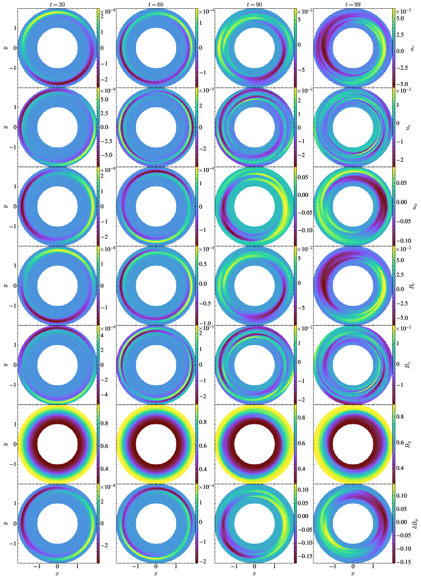
Figure 1: Slices at the mid-plane $z=0$ of selected fluid quantities (from top to bottom): the velocity components $u_{r}$, $u_{z}$, $u_{\phi}$, the magnetic field components $B_{r}$, $B_{z}$, $B_{\phi}$ and the azimuthal magnetic field perturbations $\delta B_{\phi}$, at $t=30,60,90$ and $99$ (from left to right) in the fiducial simulation Om.5_OmA.25_N1. The early linear growth phase at $t\lesssim 60$ features an $m=1$ mode, with the amplitudes of fluid quantities growing exponentially. The $m=1$ mode is later mixed with higher modes after $t\!\gtrsim\!80$, with the amplitudes reaching saturation.

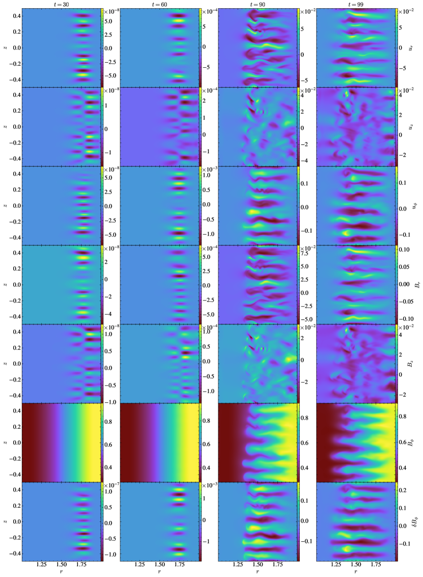
Figure 2: Slices of the $r-z$ plane at $\phi=0$, as Fig. 1. During the nonlinear growth and saturation phases at $t=90$ and $99$, horizontally aligned structures are strongly distorted and propagate toward smaller radii. The $u_{z}$ and $B_{z}$ structures appear turbulent, indicative of a secondary shear instability.

We first study the run Om.5_OmA.25_N1 as a fiducial case. Fig. 1 shows the time evolution at $t=30,60,90$ and $99$ (from left to right columns) of each velocity component ($u_{r}$, $u_{z}$ and $u_{\phi}$) and magnetic field component ($B_{r}$, $B_{z}$ and $B_{\phi}$), along with the azimuthal magnetic field perturbations ($\delta B_{\phi}\equiv B_{\phi}-\langle B_{\phi}\rangle_{\phi}$, where $\langle...\rangle_{\phi}$ denotes azimuthal averaging), in the $r-\phi$ plane. Note that the $m=1$ mode structures emerge by $t=30$ in Fig. 1, as expected for Tayler instability. The amplitudes of the $m=1$ mode grow exponentially, up to $\sim 10^{-8}$ by $t=30$ and $\sim 10^{-4}$ by $t=60$. By $t=90$ and $99$ (right two columns of Fig. 1), the amplitudes have saturated, and the $m=1$ structure has mixed together with higher $m$ modes.

Fig. 2 shows the time evolution of the same set of quantities as Fig. 1, but viewed in the $r-z$ plane. The structures on the $r$-$z$ plane are mostly horizontally aligned, with a short wavelength in the $z-$direction. Because the dominant perturbations have $m=1$, the values of $u_{r}$, $u_{z}$, etc., oscillate in time as the flow pattern propagates. In the non-linear and saturation phases, the banded structure is mostly maintained, but with a slightly longer wavelength in the $z$-direction and distorted structure. However, the $z$-components of the flow, $u_{z}$ and $B_{z}$, become highly turbulent during the non-linear saturation phase, losing the banded structure. This appears to be the result of secondary shear instabilities that develop as the instability saturates. The unstable eigenmodes are initially confined to $r\!\gtrsim\!1.5$. Simultaneously with saturation, the flow pattern migrates inward, reaching nearly the inner boundary. We will discuss the transition to the nonlinear stage and the shear instability in the following sections.

3.2 Linear growth rate

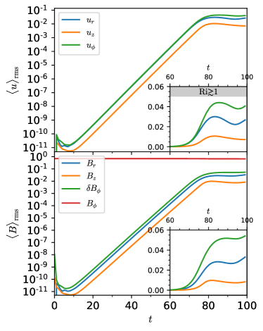
Figure 3: Time evolution of volume-averaged root-mean-squared velocities (top) and magnetic fields (bottom) in the fiducial simulation Om.5_OmA.25_N1, with zoom-in on linear scales near the non-linear stage at $t>60$. The regime where the Richardson number $\mathrm{Ri}\gtrsim 1$ (see §3.4) is shadowed in the zoom-in plot. The magnitudes of both velocities and magnetic fields grow exponentially and finally saturate at $u_{\perp}=\sqrt{u_{z}^{2}+u_{\phi}^{2}}\sim 0.05$ which corresponds to $\mathrm{Ri}\sim 1$.

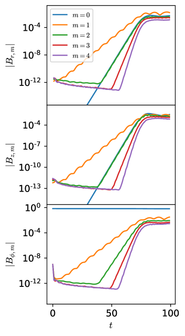
Figure 4: Time evolution of volume-averaged root-mean-squared azimuthal modes of magnetic fields $|B_{m}|$ in the fiducial simulation Om.5_OmA.25_N1. The $m=1$ mode is dominant in the linear growth phase, and higher modes start to grow at later times, e.g., the $m=0$ and $m=2$ mode grows from $t\sim 40$ at twice the rate of the $m=1$ mode.

Fig. 3 shows the time evolution of the root-mean-squared velocities (top) and magnetic fields (bottom) in the fiducial simulation Om.5_OmA.25_N1. The evolution of both velocities and magnetic fields goes through a linear growth stage for $t\sim 80$ before reaching saturation. As expected, the magnitude of $u_{z}$ is smaller than $u_{r}$ and $u_{\phi}$ by a factor of several, due to the buoyancy force that restricts motion in the $z-$direction. Similarly, $B_{z}$ remains several times smaller than $B_{r}$ or $\delta B_{\phi}$. At saturation, the perturbed field components remain more than a factor of ten weaker than the background field $B_{\phi}$, which weakens only slightly by the end of the simulation.

We further examine the growth of magnetic fields by decomposing them into different azimuthal modes with the following equation

$$\left|B_{m}\right|^{2}\equiv\left\langle\left|\frac{1}{2\pi}\int d\phi e^{im\phi}B(r,z,\phi)\right|^{2}\right\rangle_{r,z}$$ (19)

with $m$ as azimuthal mode numbers, and $\langle...\rangle_{r,z}$ denoting averaging over $r$ and $z$ under cylindrical coordinates. We plot the time evolution of the amplitudes of different modes in Fig. 4. The $m=1$ mode is dominant over higher $m$ modes in the linear growth phase, consistent with the apparent $m=1$ mode structure in Fig. 1. Modes of $m\geq 2$ start to grow at $t\sim 40$, and all modes ultimately reach saturation at $t\sim 80$. We will discuss the nonlinear coupling and saturation in §3.3 and §3.4.

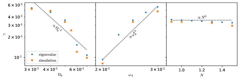
Figure 5: Linear growth rates $\gamma$ of the Tayler instability vs $\Omega_{0}$, $\omega_{\mathrm{A}}$ and $N$, given by linear eigenvalue calculations (blue dots) and measured from simulations (orange stars) with varying parameters. The linear growth rates in simulations are well-predicted by the linear eigenvalue calculations.

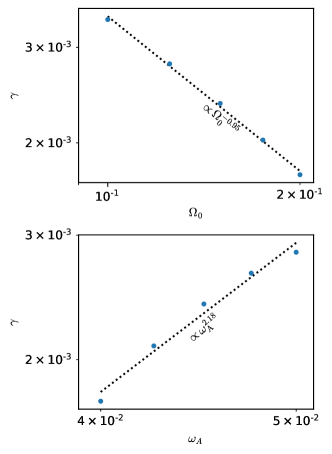
Figure 6: Linear growth rates $\gamma$ of the Tayler instability from linear eigenvalue calculations (blue dots), with much greater scale separations ( $\omega_{A}\sim 0.04$ – $0.05$, $\Omega_{0}\sim 0.1$ – $0.2$, $N=1$ and $\eta=5\times 10^{-6}$) and consequently much smaller growth rates ($\gamma\sim$ a few $\times 10^{-3}$) than the fiducial simulations. With larger scale separations between $\omega_{\mathrm{A}}$, $\Omega_{0}$ and $N$, the best power-law fits (dashed line) is roughly consistent with the theoretical prediction of $\gamma\propto\omega_{\mathrm{A}}^{2}\Omega_{0}^{-1}$ (Spruit, 1999), and the growth rates are much smaller than those in Fig. 5.

We measure the linear growth rates of the Tayler instability from simulations with varying initial-conditions parameters, including the angular frequency $\Omega_{0}$, Aflvén frequency $\omega_{\mathrm{A}}$ and Brunt-Väisälä frequency $N$. The growth rates measured from simulations (orange stars) are plotted against the eigenmodes (blue dots) of the Tayler instability setup calculated with the eigenvalue problem solver in Dedalus. The simulated linear growth rates $\gamma$ are well-predicted by the linear eigenvalue calculations, following a scaling relation of $\gamma\propto\omega_{\mathrm{A}}^{4.5}\Omega_{0}^{-2}N^{0}$ (Fig. 5). This scaling is different than expected from Spruit (1999) (see also Zahn et al. 2007 and Ma & Fuller 2019), who predicts the fastest growing modes scale as $\gamma\sim\omega_{\mathrm{A}}^{2}\Omega_{0}^{-1}$ in the limit that $\omega_{\mathrm{A}}\ll\Omega_{0}$. This occurs because our simulations are not actually in the asymptotic limit of $\omega_{\rm A}\ll\Omega\ll N$ used for the analytic estimates in those works: in Fig. 6, we further carry out linear eigenvalue calculations with larger scale separations with $\omega_{A}\sim 0.04$ – $0.05$, $\Omega_{0}\sim 0.1$ – $0.2$, $N=1$ and $\eta=5\times 10^{-6}$, and find that the obtained scaling relations of the growth rates are quite consistent with the predictions by Spruit (1999). However, the resulting growth rates are as low as a few $10^{-3}$, which are much smaller than those with fiducial parameters ($\gamma\sim$ a few $\times 10^{-1}$ in Fig. 5) and are prohibitively small for numerical simulations to follow the growth of the Tayler instability. Therefore, we stick to the fiducial parameters for the simulations even though they have limited scale separations, and bear it in mind when comparing our results with analytic estimates that the simulations are not fully in the limit of $\omega_{\rm A}\ll\Omega_{0}$ as used in many analytic works.

3.3 Nonlinear coupling

From Fig. 4, we can see that during the linear growth phase, the amplitude of the $m=1$ mode grows exponentially as expected. The $m=0$ and $m\geq 2$ modes initially decay because they are stable, but eventually they also start growing exponentially. This is a consequence of non-linear power transfer from the large amplitude $m=1$ mode to other values of $m$. From the induction equation (16), we can see that the magnetic field grows as (neglecting diffusive effects which are small in this analysis)

$$\frac{\partial\bm{B}}{\partial t}\simeq\nabla\times\left(\bm{u}\times\bm{B}\right)\,.$$ (20)

During the linear growth stage, fluctuations in $\bm{u}$ and ${\bm{B}}$ are dominated by the $m=1$ component, which has time and spatial dependence $B\propto\sin(\phi-\omega t)e^{\gamma t}$, and similar for $u$. Here $\omega$ is the real part of the frequency of the fastest growing mode, and $\gamma$ is its growth rate. Hence, to lowest order, the $m\neq 1$ components grow as

$$\frac{\partial B}{\partial t} \propto\sin^{2}(\phi-\omega t)e^{2\gamma t}$$

$$\propto\frac{1}{2}\big{[}1-\cos(2\phi-2\omega t)\big{]}e^{2\gamma t}\,.$$ (21)

for $m=0$ and $m\geq 2$ modes.

Multiplying each side of Eq. (3.3) by $\sin(m\phi)$ and integrating over volume gives the contribution to the non-linear growth of $\vec{B}$ at a desired wavenumber $m$. We see that to the lowest order, only the $m=0$ and $m=2$ modes have a non-vanishing integral, arising from the first and second terms inside the parentheses in Eq. (3.3), respectively. Hence, we see that the $m=0$ and $m=2$ modes grow at exactly twice the rate as the $m=1$ mode, as long as the $m=1$ mode has much larger amplitude. At a given time $t$, the amplitude of the non-linearly excited modes scales as $\vec{B}\propto\int\dot{\vec{B}}dt\propto B(r,z,m=1,t=0)^{2}e^{2\gamma t}$. Hence at a given time $t$, the ratio of the non-linearly excited mode to the linearly excited mode is

$$\frac{|B(m=0,2)|}{|B(m=1)|}=\kappa B(m=1)\,,$$ (22)

where $\kappa$ is a constant of proportionality that captures the non-linear coupling between modes. From Fig. 4, we estimate $\kappa\sim 0.1/B_{\phi}$, where $B_{\phi}$ is the background magnetic field strength. Hence, the non-linearly excited modes have much smaller amplitudes in the linear regime where $B(m=1)\ll B_{\phi}$.

Extending this calculation to $m>2$ requires higher chains of non-linear interaction that results in a non-linear growth rate $m\gamma$ for modes with $m\geq 2$. This scaling is verified by the growth rates and amplitudes shown in Fig. 4 in the linear regime, with $t\lesssim 70$. Hence, in the linear growth phase, we clearly see a non-linear transfer of power to smaller scales. By the time the instability saturates, the high-$m$ modes have reached amplitudes comparable to (but smaller than) the $m=1$ mode, and the weakly non-linear analysis presented above begins to break down.

3.4 Non-linear saturation

The end of linear growth and apparent saturation of the instability at around $t=80$ in our simulations is accompanied by a remarkable change in the motions and morphology of the simulation domain (see Fig. 2). This includes the appearance of turbulent non-layered structure in $u_{z}$ and $B_{z}$ (Fig. 2), as well as the inward motion of the perturbed flow.

The turbulent structure appears to stem from secondary shear instabilities. We believe the evolution is similar to the magnetized Rayleigh-Taylor instability, where the primary instability also drives opposing flows which then exhibit shear instabilities (e.g., Stone & Gardiner, 2007). For the Tayler instability as we consider here, buoyancy provides a restoring force in the $z$ direction. The horizontal flows driven by the instability will become unstable to secondary Kelvin-Helmholtz instabilities when

$$k_{z}u_{\perp}\gtrsim 2N\,,$$ (23)

where $u_{\perp}=\sqrt{u_{r}^{2}+u_{\phi}^{2}}$ is the fluid velocity perpendicular to $\hat{z}$. Near the end of the simulation, the dominant modes have roughly seven wavelengths in the $z-$direction and hence $k_{z}\sim 40$. Therefore in our simulations with $N=1$, we expect shear instabilities to occur when $u_{\perp}\sim u_{\phi}\gtrsim 0.05$. Indeed, Fig. 3 shows that the system reaches its saturated state very near this scale, and that this saturation is accompanied by turbulence shown in Fig. 2. Despite the shear instabilities, $u_{r}$, $u_{\phi}$, $B_{r}$, and $\delta B_{\phi}$ all maintain a banded structure in the $z$-direction, and they also maintain a predominantly $m=1$ azimuthal structure.

At the same time that secondary instabilities develop, the unstable region also “migrates inward”. During linear growth, the instability is restricted to large radii with $r\gtrsim 1.5$, because the Tayler instability only occurs in the outer part of the domain where the background magnetic field is stronger. As the instability saturates around $t=80$, however, the unstable motions and magnetic field perturbations move inwards to the inner boundary at $r=1$. The inward-moving fingers have a predominantly $m=1$ azimuthal structure and feature inward radial motion at alternating heights, accompanied by an outward return flow in between. Their structures resemble convective plumes/fingers seen in the early phases of convective/thermohaline instability.

We posit that the secondary instabilities cause saturation both by dissipating energy from the growing modes, and by allowing for the inward motion of the instability. Once the fluid elements obtain velocities large enough to overcome the Richardson criterion of Eq. (23), inertial forces become comparable to buoyancy forces, and fluid elements can flow with fewer constrictions. This may allow for circulation to smaller radii that was previously prevented by buoyancy/Coriolis forces. It is also possible that non-linear inertial terms effectively change the linear dispersion relation, allowing unstable motions to grow at smaller radii. Future work should investigate this effect in detail, and determine whether latitudinal migration of the Tayler instability could occur in real stars.

3.5 Dynamo action

A major question regarding the Tayler-Spruit dynamo is whether a dynamo actually occurs. In the picture advanced by Spruit (2002), differential rotation amplifies $B_{\phi}$ by winding up a weak poloidal field. The dynamo loop is supposed to be closed by the amplification of the poloidal field via the unstable motions associated with Tayler instability. However, as pointed out by Zahn et al. (2007) (see also Fuller et al. 2019), the unstable motions are $m=1$ and do not directly produce an axisymmetric component of the poloidal field that is needed for amplification of $B_{\phi}$ via differential rotation. Hence, a non-linear coupling process is needed to amplify the axisymmetric poloidal field, and this step of the dynamo is poorly understood.

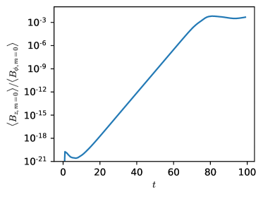
Figure 7: Time evolution of the ratio of axisymmetric ($m=0$ mode) $B_{z}$ to $B_{\phi}$ components from the simulation Om.5_OmA.25_N1, demonstrating the non-linear induction process needed to amplify the axisymmetric poloidal field to close a dynamo loop.

Fig. 7 shows the growth of the axisymmetric component of $B_{z}$, $B_{z,m=0}$, which is the poloidal component of the field needed to be generated by the Tayler instability in order for a dynamo to occur. Our simulations do not include differential rotation and thus cannot capture the winding of $B_{z,m=0}$ needed to close the dynamo loop. However, our simulations clearly demonstrate non-linear amplification of $B_{z,m=0}$, as also discussed in Section 3.3. We have verified that the proportionality of the scaling $B_{z}/B_{\phi}\sim\omega_{\rm A}/N$ predicted by Spruit (2002) and Fuller et al. (2019) roughly holds, but with a much smaller normalization factor of $B_{z}\sim 10^{-2}B_{\phi}$ for the saturated state of our simulations, rather than the predicted $B_{z}\sim(\omega_{\rm A}/N)B_{\phi}\sim 1/4B_{\phi}$, i.e., the axisymmetric component of $B_{z}$ in our simulations saturates at much lower values than predicted by the scaling relation. However, both of those models are based on dynamos sustained by energy input by shear, which cannot occur in our simulations, so the disagreement is not surprising.

Future work will be necessary to understand the saturated state of the Tayler-Spruit dynamo, but our simulations do indicate that a dynamo based on non-linear induction can greatly amplify the axisymmetric component of the poloidal field.

3.6 Scaling Relations

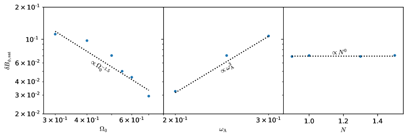
Figure 8: Saturated RMS values of $\delta B_{\phi}$ as a function of $\Omega_{0}$, $\omega_{\mathrm{A}}$ and $N$, measured from simulations with varying parameters at the saturation stage. The saturated magnitudes of $\delta B_{\phi}$ strongly correlate with the $\Omega_{0}$ and $\omega_{\mathrm{A}}$, and they are approximately independent of $N$ as expected.

A key result of our simulations is how the properties of the saturated state depend on input parameters ($\omega_{\rm A}$, $\Omega_{0}$, etc.). Fig. 8 shows how the mean amplitude of the magnetic field perturbations in the saturated state, $\delta B_{\phi,{\rm sat}}$, scale with $\Omega_{0}$, $\omega_{\rm A}$, and $N$. The saturated values of $\delta B_{\phi,{\rm sat}}$ scale strongly with rotation rate and initial magnetic field, with $\delta B_{\phi,{\rm sat}}\propto\Omega_{0}^{-1.5}$ and $\delta B_{\phi,{\rm sat}}\propto\omega_{\rm A}^{3}$, and almost no dependence on $N$. These scalings are similar to (but slightly weaker than) the linear growth rate scaling presented in Fig. 5.

Based on the discussion above, we believe the instability saturates in our simulations due to secondary shear instabilities. For the large-scale growing modes with $m\sim 1$, the non-linear inertial term $(\bm{u}\cdot\nabla){\bm{u}}$ produces an effective damping rate of order $\gamma_{\rm NL}\sim 2\pi u_{\phi}/r$. In the rapidly rotating limit, we expect $u_{\phi}\propto(\omega_{\rm A}/\Omega_{0})\delta B_{\phi,{\rm sat}}$ (Spruit, 2002; Fuller et al., 2019), so the non-linear damping rate will scale as $\gamma_{\rm NL}\propto\delta B_{\phi,{\rm sat}}(\omega_{\rm A}/\Omega)$. Setting this equal to the linear growth rate, which scales as $\gamma\propto\omega_{\rm A}^{4.5}/\Omega_{0}^{2}$ (Fig. 5) yields an expected scaling of the non-linear saturation amplitude of $\delta B_{\phi,{\rm sat}}\propto\omega_{\rm A}^{3.5}/\Omega_{0}$, similar to the scaling Fig. 8. The slight mismatch between these scaling laws could stem from the small dynamic range covered by our simulations, or the fact that they are not quite in the rapidly rotating limit.

Fuller et al. (2019) argued that Tayler instability saturates via weak magnetic turbulence with a non-linear damping rate of $\gamma_{\rm NL}\sim\delta\omega_{\rm A}\propto\delta B_{\phi,{\rm sat}}$. Setting this expectation equal to the linear growth rates would entail $\delta B_{\phi,{\rm sat}}\propto\omega_{\rm A}^{4.5}/\Omega_{0}^{2}$, steeper than the scalings shown in Fig. 8. Hence, it appears that our simulations do not saturate via weak magnetic turbulence as predicted by Fuller et al. (2019). However, in the next section, we discuss why the saturation mechanism is likely to be different when the Tayler instability operates in stellar interiors.

4 Discussion and Conclusion

Although secondary shear instabilities appear to saturate the Tayler instability in our simulations, it is likely that a different mechanism will operate in real stars. Fuller et al. (2019) predict that non-linear Alfvén wave dissipation produces damping at the rate $\gamma_{\rm NL}\sim\delta v_{\rm A}/r$, which in our units equates to $\gamma_{\rm NL}\sim\delta B_{\phi}/r\sim 0.04$ in the saturated state. The dimensionless growth rate (Fig. 5) is larger than this, roughly 0.4 for the fiducial simulation Om.5_OmA.25_N1. This indicates that the instability saturates via shear instabilities before it reaches an amplitude high enough for Alfvén wave dissipation to dominate. In a real star, however, Alfvén wave dissipation would likely occur before shear instability. As described above, the dissipation rate from shear instabilities is $\gamma_{\rm NL}\sim 2\pi u_{\phi}/r$, and we expect $u_{\phi}\sim(\omega_{\rm A}/\Omega_{0})\delta v_{\rm A}$ in the limit $\omega_{\rm A}/\Omega_{0}\ll 1$ applicable to real stars. Because our simulations only reach $\omega_{\rm A}/\Omega_{0}\sim 1/2$, dissipation via shear instability and Alfvénic dissipation are comparable, and evidently, shear instability is more important by a factor of a few. But in a real star with $\omega_{\rm A}/\Omega_{0}\ll 1$, shear instabilities become less important, and Alfvénic dissipation is expected to dominate. Hence, our simulations cannot grow to an amplitude high enough to test the prediction of Fuller et al. (2019), because of the small ratio of $\Omega$ to $\omega_{\rm A}$. Future work should push towards larger scale separations to better test these predictions.

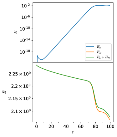
Figure 9: Time evolution of the volume-integrated kinetic $E_{k}$ (blue), magnetic $E_{B}$ (orange) and total $E_{k}+E_{B}$ (green) energies from the fiducial simulation Om.5_OmA.25_N1. Together with the order-of-magnitude growth of the kinetic energy driven by the Tayler instability, the magnetic energy slightly dissipates at a rate roughly consistent with the prediction of $\sim\gamma|\delta B_{\phi}|$, where $\gamma$ is the growth rate of the Tayler instability.

To determine whether Alfvén wave damping or shear instability will saturate Tayler instability, we can determine which mechanism requires a lower threshold to operate. As described above, shear instability requires $u_{\perp}\!\sim\!2N/k_{z}$. The fastest growing modes have $k_{z}^{2}\eta\!\sim\!\omega_{\rm A}^{2}/\Omega$, so shear instability operates when $u_{\perp}\!\sim 2(\Omega\eta)^{1/2}N/\omega_{\rm A}$. In contrast, Alfvén wave damping saturates the instability when $\delta v_{\rm A}\!\sim\!r\omega_{\rm A}^{2}/\Omega$. Using $\delta v_{\rm A}\!\sim\!(\Omega/\omega_{\rm A})u_{\perp}$, the corresponding velocity amplitude for Alfvén wave damping is $u_{\perp}\!\sim\!r\omega_{\rm A}^{3}/\Omega^{2}$. Hence, Alfvén wave damping will dominate when $r\omega_{\rm A}^{3}/\Omega^{2}\!\lesssim\!2(\Omega\eta)^{1/2}N/\omega_{\rm A}$, which translates to $\omega_{\rm A}/\Omega\!\lesssim\!(N/\Omega)^{1/4}(\eta/r^{2}\Omega)^{1/8}\equiv x$. We note that the instability growth criterion is $\omega_{\rm A}/\Omega\!\gtrsim\!(N/\Omega)^{1/2}(\eta/r^{2}\Omega)^{1/4}=x^{2}$. Hence, Alfvén wave damping is expected to cause saturation when $x^{2}\!\lesssim\!\omega_{\rm A}/\Omega\!\lesssim\!x$, while shear instability is expected to cause saturation when $\omega_{\rm A}/\Omega\!\gtrsim\!x$. Our simulations have $\omega_{\rm A}/\Omega\!\approx\!0.5$, and $x\!\approx\!0.3$, hence we expect them to saturate via shear instability. However, simulations that reach lower values of $\omega_{\rm A}/\Omega$ are expected to exhibit saturation of the instability via Alfvén wave damping. We hope to explore this possibility in future work.

Another argument against shear instability being important in real stars is as follows. According to the saturated state of Fuller et al. (2019), the value of $k_{z}u_{\perp}$ reaches $k_{z}u_{\perp}\sim q\Omega^{2}/N$, where $q=d\ln\Omega/d\ln z$ is the dimensionless shear. This is much smaller than $N$ unless $q\Omega^{2}\gtrsim N^{2}$, which cannot occur in real stars, since a background state with $q\Omega^{2}\gtrsim N^{2}$ would already satisfy the Richardson criterion for overturning the stratification. Therefore, at the saturated state due to Alfvén wave dissipation, the value of $k_{z}u_{\perp}$ would be much less than required to overturn the stratification and cause shear instability. Simulations including shear and pushing to smaller ratios of $\Omega_{0}/N$ will be needed to test this prediction.

Our simulations appear to disagree with the model of Spruit (2002), in which turbulent dissipation in the saturated state dissipates magnetic energy at the rate $\dot{E}\sim\gamma B_{\phi}^{2}$, where $\gamma$ is the linear growth rate (equal to the non-linear damping rate) of the Tayler instability. Even though our saturated state is somewhat turbulent, it does not dissipate magnetic energy at this rate, as can be seen from the bottom panel of Fig. 9. Since the growth rate of the instability is $\gamma\sim 0.4$, this would imply that all of the magnetic energy would dissipate within a time span of $\Delta t\sim 2.5$. In contrast, Fig. 9 shows that the magnetic energy only decreases by $\sim$10% in the final $\Delta t=20$ of our simulation, corresponding to a magnetic energy dissipation rate of $\dot{E}_{B}\sim 2\times 10^{-2}$ as shown in Fig. 10. This corresponds to magnetic energy dissipation $\sim$2 orders of magnitude slower than $\dot{E}\sim\gamma B_{\phi}^{2}$. Fig. 10 also shows that kinetic energy dissipation is negligible relative to magnetic energy dissipation. However, we note that our imposed background field $B_{\phi}$ is ordered (uniform in the $z-$direction), and a field built up by a dynamo could be disordered, allowing for more magnetic energy dissipation. Also, our boundary conditions prevent $B_{\phi}$ from being totally erased, which may limit the turbulent dissipation of $B_{\phi}$. Future work with different initial conditions and boundary conditions will shed light on this issue.

Shortly before this paper was submitted, Petitdemange et al. (2023) presented a suite of dynamo simulations driven by differential rotation and exhibiting the Tayler instability in a spherical shell. Since their methods were very different from ours, we do not attempt a direct comparison with our results. In their setup, shear was created by enforcing the outer boundaries to rotate at different rates, though this also created Ekman boundary layer effects and a related “weak dynamo” that complicated the analysis. The Tayler instability was triggered once the magnetic field generated by the weak dynamo exceeded the threshold derived from linear theory. The saturation mechanism of the Tayler instability was not clear from that work, but the magnetic torques in the saturated state appeared to scale according to the predictions of (Spruit, 2002). However, most of those simulations appeared to have $\Omega/N\sim 1$, where the predictions of (Spruit, 2002) and Fuller et al. (2019) are similar. While the work of Petitdemange et al. (2023) is a great leap forward in modeling the Tayler instability, our understanding of the saturation mechanism and magnetic torques in real stellar interiors remains incomplete.

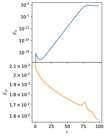
Figure 10: Time evolution of the volume-integrated kinetic $\dot{E}_{k}$ (top) and magnetic $\dot{E}_{B}$ (bottom) energy dissipation rates from the fiducial simulation Om.5_OmA.25_N1.

4.1 Conclusion

In this study, we perform three-dimensional MHD simulations of the Tayler instability in a cylindrical annulus, with strong buoyancy and Coriolis forces incorporated to mimic realistic stellar environments. The simulations are initialized with a strong toroidal field which is in magnetostatic equilibrium. We explore a range of parameter space by varying the angular velocities $\Omega_{0}$, Alfvén frequency $\omega_{\mathrm{A}}$ and Brunt-Brunt-Väisälä frequency $N$, with the the correct order of $N>\Omega_{0}>\omega_{\mathrm{A}}$ that typically exists in realistic stars.

We find that as theoretically expected, the initial conditions adopted are unstable to the Taylor instability. The $m=1$ mode clearly dominates the linear growth of the instability, and the linear growth rates are well-predicted by the linear eigenvalue calculations. The linear growth phase is later accompanied by a non-linear coupling between the $m=1$ and other azimuthal modes, leading to the growth of $m=0$ and $m\geq 2$ modes. The $m=0$ component of the poloidal field is amplified by the instability, signaling a dynamo that can regenerate the poloidal field as necessary for the Tayler-Spruit dynamo to occur.

Both the linear growth rates and the saturated magnetic field measured in the simulations scale strongly with angular velocities $\Omega_{0}$ and the Alfvén frequencies $\omega_{\mathrm{A}}$ parameters, and are nearly independent of $N$. While this has been predicted from linear theory and non-linear saturation models, the scaling in our simulations is steeper, due to the fact they are not in the asymptotic limit of $\omega_{\rm A}\ll\Omega_{0}\ll N$ assumed in analytic work. With greater scale separations, the linear eigenvalue calculations are able to replicate the scaling relations of $\gamma\propto\omega_{\mathrm{A}}^{2}\Omega_{0}^{-1}$ predicted by analytic work, even though the resulted growth rates are prohibitively too small to simulate numerically.

The linear growth is ultimately followed by a non-linear saturation of the instability, which appears to be caused by secondary shear instabilities. The saturation is also accompanied by an inward migration of unstable motions, whose cause is not clear. We argued that saturation via secondary shear instability is unlikely to operate in real stars where the stratification is greater (preventing shear instabilities), and where Alfvén wave damping becomes more important due to the larger separation of scales than we could achieve in our simulations. During the saturated phase, energy is dissipated primarily through magnetic diffusion. However, it is dissipated much more slowly than predicted by the model of Spruit (2002), likely entailing the instability can grow to larger amplitudes as expected in the model of Fuller et al. (2019).

Certain caveats apply to this study. First, due to limited computational capability, the scale separations between the parameters $\Omega_{0}$, $\omega_{\mathrm{A}}$ and $N$ are much less than that in real stars, the scaling relations obtained from simulations might differ from what occurs in realistic stellar environments. Second, although amplification of the axisymmetric poloidal magnetic field is observed in the simulations, differential rotation is not included in our simulations, which is necessary to close the loop of the Tayler-Spruit dynamo. We thus cannot directly test theoretical predictions of the angular momentum transport caused by this dynamo, leaving room for improvement in future work.

Data Availability

The data supporting the plots within this article are available on reasonable request to the corresponding author.

References

- Beck et al. (2012) Beck P. G., et al., 2012, Nature, 481, 55
- Belkacem et al. (2015) Belkacem K., et al., 2015, A&A, 579, A31
- Benomar et al. (2015) Benomar O., Takata M., Shibahashi H., Ceillier T., García R. A., 2015, MNRAS, 452, 2654
- Braithwaite (2006) Braithwaite J., 2006, A&A, 449, 451
- Burns et al. (2020) Burns K. J., Vasil G. M., Oishi J. S., Lecoanet D., Brown B. P., 2020, Physical Review Research, 2, 023068
- Cantiello et al. (2014) Cantiello M., Mankovich C., Bildsten L., Christensen-Dalsgaard J., Paxton B., 2014, ApJ, 788, 93
- Couston et al. (2018) Couston L.-A., Lecoanet D., Favier B., Le Bars M., 2018, Phys. Rev. Lett., 120, 244505
- Deheuvels et al. (2014) Deheuvels S., et al., 2014, A&A, 564, A27
- Deheuvels et al. (2015) Deheuvels S., Ballot J., Beck P. G., Mosser B., Østensen R., García R. A., Goupil M. J., 2015, A&A, 580, A96
- Eggenberger et al. (2017) Eggenberger P., et al., 2017, A&A, 599, A18
- Fuller et al. (2014) Fuller J., Lecoanet D., Cantiello M., Brown B., 2014, ApJ, 796, 17
- Fuller et al. (2019) Fuller J., Piro A. L., Jermyn A. S., 2019, MNRAS, 485, 3661
- Gehan et al. (2018) Gehan C., Mosser B., Michel E., Samadi R., Kallinger T., 2018, A&A, 616, A24
- Gellert et al. (2008) Gellert M., Rüdiger G., Elstner D., 2008, A&A, 479, L33
- Goldstein et al. (2019) Goldstein J., Townsend R. H. D., Zweibel E. G., 2019, ApJ, 881, 66
- Guerrero et al. (2019) Guerrero G., Del Sordo F., Bonanno A., Smolarkiewicz P. K., 2019, MNRAS, p. 2461
- Hermes et al. (2017) Hermes J. J., et al., 2017, ApJS, 232, 23
- Hunter (2007) Hunter J. D., 2007, Computing in science & engineering, 9, 90
- Kurtz et al. (2014) Kurtz D. W., Saio H., Takata M., Shibahashi H., Murphy S. J., Sekii T., 2014, MNRAS, 444, 102
- Lecoanet et al. (2015) Lecoanet D., Le Bars M., Burns K. J., Vasil G. M., Brown B. P., Quataert E., Oishi J. S., 2015, Phys. Rev. E, 91, 063016
- Lecoanet et al. (2017) Lecoanet D., Vasil G. M., Fuller J., Cantiello M., Burns K. J., 2017, MNRAS, 466, 2181
- Ma & Fuller (2019) Ma L., Fuller J., 2019, MNRAS, 488, 4338
- Mosser et al. (2012) Mosser B., et al., 2012, A&A, 548, A10
- Oliphant (2007) Oliphant T. E., 2007, Computing in Science & Engineering, 9, 10
- Ouazzani et al. (2019) Ouazzani R.-M., Marques J., Goupil M.-J., Christophe S., Antoci V., Salmon S., Ballot J., 2019, Astronomy & Astrophysics, 626, A121
- Petitdemange et al. (2023) Petitdemange L., Marcotte F., Gissinger C., 2023, Science, 379, 300
- Saio et al. (2015) Saio H., Kurtz D. W., Takata M., Shibahashi H., Murphy S. J., Sekii T., Bedding T. R., 2015, MNRAS, 447, 3264
- Spada et al. (2016) Spada F., Gellert M., Arlt R., Deheuvels S., 2016, A&A, 589, A23
- Spruit (1999) Spruit H. C., 1999, A&A, 349, 189
- Spruit (2002) Spruit H. C., 2002, A&A, 381, 923
- Stone & Gardiner (2007) Stone J. M., Gardiner T., 2007, Physics of Fluids, 19, 094104
- Tayler (1973) Tayler R. J., 1973, MNRAS, 161, 365
- Triana et al. (2017) Triana S. A., Corsaro E., De Ridder J., Bonanno A., Pérez Hernández F., García R. A., 2017, A&A, 602, A62
- Turk et al. (2010) Turk M. J., Smith B. D., Oishi J. S., Skory S., Skillman S. W., Abel T., Norman M. L., 2010, The Astrophysical Journal Supplement Series, 192, 9
- Van Der Walt et al. (2011) Van Der Walt S., Colbert S. C., Varoquaux G., 2011, Computing in Science & Engineering, 13, 22
- Van Reeth et al. (2018) Van Reeth T., et al., 2018, Astronomy & Astrophysics, 618, A24
- Weber et al. (2015) Weber N., Galindo V., Stefani F., Weier T., 2015, New Journal of Physics, 17, 113013
- Zahn et al. (2007) Zahn J.-P., Brun A. S., Mathis S., 2007, A&A, 474, 145