Robust Inference of Manifold Density and Geometry
by Doubly Stochastic Scaling

Abstract

The Gaussian kernel and its traditional normalizations (e.g., row-stochastic) are popular approaches for assessing similarities between data points. Yet, they can be inaccurate under high-dimensional noise, especially if the noise magnitude varies considerably across the data, e.g., under heteroskedasticity or outliers. In this work, we investigate a more robust alternative – the doubly stochastic normalization of the Gaussian kernel. We consider a setting where points are sampled from an unknown density on a low-dimensional manifold embedded in high-dimensional space and corrupted by possibly strong, non-identically distributed, sub-Gaussian noise. We establish that the doubly stochastic affinity matrix and its scaling factors concentrate around certain population forms, and provide corresponding finite-sample probabilistic error bounds. We then utilize these results to develop several tools for robust inference under general high-dimensional noise. First, we derive a robust density estimator that reliably infers the underlying sampling density and can substantially outperform the standard kernel density estimator under heteroskedasticity and outliers. Second, we obtain estimators for the pointwise noise magnitudes, the pointwise signal magnitudes, and the pairwise Euclidean distances between clean data points. Lastly, we derive robust graph Laplacian normalizations that accurately approximate various manifold Laplacians, including the Laplace Beltrami operator, improving over traditional normalizations in noisy settings. We exemplify our results in simulations and on real single-cell RNA-sequencing data. For the latter, we show that in contrast to traditional methods, our approach is robust to variability in technical noise levels across cell types.

1 Introduction

1.1 Traditional normalizations of the Gaussian kernel

Many popular techniques for clustering, manifold learning, visualization, and semi-supervised learning, begin by learning similarities between observations. The learned similarities then form an affinity matrix that describes a weighted graph, which is further processed and analyzed according to the required task. A popular approach to construct an affinity matrix from the data is to evaluate the Gaussian kernel with pairwise Euclidean distances. Specifically, letting $y_{1},\ldots,y_{n}\in\mathbb{R}^{m}$ be a collection of given data points, we define the Gaussian kernel $\mathcal{K}_{\epsilon}:\mathbb{R}^{m}\times\mathbb{R}^{m}\rightarrow\mathbb{R}_{+}$ and the resulting kernel matrix $K\in\mathbb{R}^{n\times n}$ as

$${K}_{i,j}=\begin{dcases}{\mathcal{K}_{\epsilon}({y}_{i},{y}_{j})},&i\neq j,\\ 0,&i=j,\end{dcases},\qquad\qquad\mathcal{K}_{\epsilon}(y_{i},y_{j})=\operatorname{exp}\left\{-\frac{\|y_{i}-y_{j}\|_{2}^{2}}{\epsilon}\right\},$$ (1)

for $i,j=1,\ldots,n$, where $\epsilon>0$ is a tunable bandwidth parameter. Here we adopt the version of the kernel matrix $K$ whose main diagonal is zeroed out, namely with no self-loops in the graph described by $K$. This choice will be further motivated from the viewpoint of noise robustness in Section 1.3.

The kernel matrix $K$ is often normalized to attain certain favorable properties. For instance, a popular choice is to divide each row of $K$ by its sum to make it a transition probability matrix. Generally, a family of normalizations that underlies many methods can be expressed by ${P}^{(\alpha)}\in\mathbb{R}^{n\times n}$ or $\hat{P}^{(\alpha)}\in\mathbb{R}^{n\times n}$ given by

$$\hat{P}^{(\alpha)}_{i,j}=\frac{{P}^{(\alpha)}_{i,j}}{\sum_{j=1}^{n}{P}^{(\alpha)}_{i,j}},\qquad\qquad{P}^{(\alpha)}=D^{-\alpha}KD^{-\alpha},\qquad\qquad D_{i,i}=\sum_{j=1}^{n}K_{i,j},$$ (2)

where $\alpha\in[0,1]$ is a parameter of the normalization, and $D\in\mathbb{R}^{n\times n}$ is a diagonal matrix whose main diagonal holds the degrees of the nodes in the weighted graph represented by $K$. If $\alpha=0$, then $\hat{P}^{(\alpha)}$ describes the popular row-stochastic normalization $D^{-1}K$, and if $\alpha=0.5$, then $P^{(\alpha)}$ describes its symmetric variant $D^{-1/2}KD^{-1/2}$. These normalizations have been utilized and extensively studied in the context of clustering [65, 54, 62, 77, 28, 74], non-linear dimensionality reduction (or manifold learning) [6, 17, 53, 47], image denoising [11, 55, 51, 44, 68], and graph-based signal processing and supervised-learning [66, 18, 31, 22, 10].

An important theoretical aspect of various normalizations is the convergence of the corresponding graph Laplacian to a differential operator as $n\rightarrow\infty$ and $\epsilon\rightarrow 0$, typically under the assumption that the points $y_{1},\ldots,y_{n}$ are sampled from a low-dimensional Riemannian manifold $\mathcal{M}$ embedded in $\mathbb{R}^{m}$; see [67, 32, 73, 12, 24, 15] and references therein. The family of normalizations in (2) was proposed in the Diffusion Maps paper [17], where it was shown that a population analogue (i.e., a continuous surrogate in the limit $n\rightarrow\infty$) of the graph Laplacian $I_{n}-\hat{P}^{(\alpha)}$ converges to a certain differential operator parametrized by $\alpha$; see Section 3.3 for more details. This operator is particularly appealing from the viewpoint of diffusion on the manifold $\mathcal{M}$; in the case of $\alpha=1$, this operator is precisely the Laplace-Beltrami operator [29], which determines the solution to the heat equation and encodes the intrinsic geometry of the manifold regardless of the sampling density. Note that the parameter $\alpha$ in (2) determines the entrywise power of the degree matrix $D$, whose diagonal entries are $\sum_{j=1,\;j\neq i}^{n}\mathcal{K}_{\epsilon}(y_{i},y_{j})$, which can be interpreted as a kernel density estimator evaluated at the sample points $y_{1},\ldots,y_{n}$ [56, 58]. Indeed, $\alpha$ controls the influence of the sampling density on the resulting affinity matrix and its spectral behavior [17].

1.2 The doubly stochastic normalization

An alternative normalization of $K$ that is not covered by $\hat{P}^{(\alpha)}$ or $P^{(\alpha)}$ of (2) is the doubly stochastic normalization [82, 83, 50, 80]

$$W_{i,j}=d_{i}{K}_{i,j}d_{j},\qquad\qquad\sum_{j=1}^{n}W_{i,j}=1,$$ (3)

for $i=1,\ldots,n$, where $d_{1},\ldots,d_{n}>0$ are the scaling factors of ${K}$. Since the resulting $W$ is symmetric and stochastic (i.e., each row sums to $1$), it is also doubly stochastic. The problem of finding $\mathbf{d}=[d_{1},\ldots,d_{n}]>0$ is known as matrix scaling, and has been extensively studied in the literature; see [3, 35] and references therein. In the case of (3), the scaling factors are guaranteed to exist and are unique for $n>2$ since ${K}$ is fully indecomposable (see Lemma 1 in [43]). Although the scaling factors $\mathbf{d}$ do not admit a closed-form solution, they can be found numerically, e.g., by the classical Sinkhorn-Knopp algorithm [69], convex optimization [2], or algorithms specialized for symmetric matrices [41, 80]. The doubly stochastic normalization is also closely related to entropic optimal transport [21, 57]. In particular, $W_{i,j}$ is the optimal transport plan between $y_{i}$ and $y_{j}$ according to the squared Euclidean distance loss with an entropic regularization term weighted by $\epsilon$ (see Proposition 2 in [43]).

Doubly stochastic affinity matrices proved useful for various tasks such as clustering [83, 5, 79, 45, 1, 23, 13], manifold learning [50, 80, 14], image denoising [52], and graph matching [19], often exhibiting more stable behavior and outperforming traditional normalizations. We note that requiring an affinity matrix to be doubly stochastic is appealing from a geometric perspective since the heat kernel on a compact Riemannian manifold – an operator describing affinities between points according to the intrinsic geometry – is always doubly stochastic [29].

In the context of manifold learning, the doubly stochastic normalization was recently investigated in [50, 80, 14]. Specifically, [50] analyzed a population setting where the scaling equation (3) is replaced with a more general family of integral equations parametrized by $\alpha$ (see eq. (5) in Section 2 for the special case of $\alpha=0.5$). It was shown that the limiting differential operator can be made the same as for the traditional normalization $\hat{P}^{(\alpha)}$ from (2) as $\epsilon\rightarrow 0$ for any $\alpha\in[0,1]$. In a different direction, [80] focused on the case where the manifold is a torus, and derived spectral convergence rates for $W$ as $n\rightarrow\infty$ and $\epsilon\rightarrow 0$, showing that the doubly stochastic normalization admits an improved bias error term compared to the traditional normalization in (2) when $\alpha=0.5$. Lastly, [14] investigated a regularized version of the scaling equation (3) where the scaling factors are lower-bounded, and established operator convergence rates of the corresponding graph Laplacian to the same operator as for $\hat{P}^{(0.5)}$ as $n\rightarrow\infty$ and $\epsilon\rightarrow 0$ on general manifolds. We note that theoretical investigation of the doubly stochastic normalization is typically more challenging than that of more traditional normalizations, particularly due to the implicit and nonlinear nature of the scaling equation (3) and its population analogue (which is a nonlinear integral equation).

1.3 The influence of noise

Modern experimental procedures such as single-cell RNA-sequencing (scRNA-seq) [9, 36, 39], cryo-electron microscopy [4, 63, 33], and calcium imaging [49, 59, 46], to name a few, produce large datasets of high-dimensional observations often corrupted by strong noise. In such cases, the classical theoretical setup where data points reside on, or near, a low-dimensional manifold can be highly inaccurate. To model noisy data, we consider

$${y}_{i}={x}_{i}+\eta_{i},$$ (4)

where $x_{1},\ldots,x_{n}$ are the underlying clean observations and $\eta_{1},\ldots,\eta_{n}\in\mathbb{R}^{m}$ are independent noise random vectors with zero means (to be specified in detail later on).

For identically distributed noise vectors $\{\eta_{i}\}_{i=1}^{n}$, the influence of noise on pairwise Euclidean distances and the entries of a kernel matrix was derived in [25]. Specifically, if the noise magnitudes $\|\eta_{i}\|_{2}^{2}$ concentrate well in high dimension around a global constant $c$, it was shown that $\|{y}_{i}-{y}_{j}\|_{2}^{2}\approx\|{x}_{i}-{x}_{j}\|_{2}^{2}+2c$ for all $i\neq j$. Consequently, the noisy Gaussian kernel $\mathcal{K}_{\epsilon}({y}_{i},{y}_{j})$ is biased for $i\neq j$ by a global multiplicative factor. Since this factor does not exist on the main diagonal of the Gaussian kernel matrix, it is advantageous to zero it out (as done in $K$ from (1)). This way, the multiplicative factor cancels out automatically through the traditional normalization $\hat{P}^{(\alpha)}$ (for any $\alpha$) or $P^{(\alpha)}$ with $\alpha=0.5$; see [26] for more details.

In many applications, the noise characteristics vary considerably across the data due to heteroskedasticity and outliers. In particular, heteroskedastic noise is prevalent in applications involving count or nonnegative data, typically modeled by, e.g., Poisson, binomial, negative binomial, or gamma distributions, whose variances inherently depend on their means, which can vary substantially across the data. Notable examples for such data are network traffic analysis [64], photon imaging [60], document topic modeling [78], scRNA-seq [30], and high-throughput chromosome conformation capture [37], among many others. Heteroskedastic noise also arises in natural image processing due to spatial pixel clipping [27] and in experimental procedures where conditions vary during data acquisition, such as in spectrophotometry and atmospheric data collection [16, 71]. Besides natural heteroskedasticity, experimental data often include outlier observations with abnormal noise distributions due to, e.g., abrupt deformations or technical errors during acquisition and storage. Consequently, to better understand the possible advantages of doubly stochastic normalization, it is important to investigate it under general non-identically distributed noise that supports heteroskedasticity and outliers.

If the noise vectors $\{\eta_{i}\}_{i=1}^{n}$ are not identically distributed or if $\|\eta_{i}\|_{2}^{2}$ do not concentrate well around a global constant, then the noisy Euclidean distances $\|{y}_{i}-{y}_{j}\|_{2}^{2}$ can be corrupted in a nontrivial way. In such cases, as demonstrated in [43], the Gaussian kernel and several of its traditional normalizations can behave unexpectedly and incorrectly assess the similarities between data points. On the other hand, [43] also shows that the doubly stochastic normalization is robust to non-identically distributed high-dimensional noise. Specifically, under suitable conditions on the noise, and if $\epsilon$ and $n$ are fixed while $m$ is growing, ${W}$ converges pointwise in probability to its clean counterpart, even if the noise magnitudes $\|\eta_{i}\|_{2}^{2}$ are comparable to the signal magnitudes $\|x_{i}\|_{2}^{2}$ and fluctuate considerably. While this result highlights an important advantage of the doubly stochastic normalization, it does not account for the sample size $n$ nor the bandwidth $\epsilon$. Hence, it remains unclear what is the population interpretation of the doubly stochastic normalization under noise in terms of the sampling density and the underlying geometry.

1.4 Our results and contributions

In this work, we consider a setting where $x_{1},\ldots,x_{n}$ are sampled from a low-dimensional manifold embedded in $\mathbb{R}^{m}$, and $\eta_{1},\ldots,\eta_{n}$ are sampled from non-identically distributed sub-Gaussian noise that allows for heteroskedasticity and outliers. Our analysis is carried out in a high-dimensional regime in which the noisy Euclidean distances satisfy $\|y_{i}-y_{j}\|_{2}^{2}=\|x_{i}-x_{j}\|_{2}^{2}+\|\eta_{i}\|_{2}^{2}+\|\eta_{j}\|_{2}^{2}+{o}(1)$, where $\|\eta_{i}\|_{2}^{2}$ are unknown and can be large, and the ${o}(1)$ term is vanishing as $m\rightarrow\infty$ but is explicitly accounted for. Our main contributions are two-fold. First, we characterize the pointwise behavior of the scaling factors $\mathbf{d}$ and the scaled matrix $W$ in terms of the quantities in our setup for large $m,n$ and small $\epsilon$; see Section 2. Second, we build on these results to infer various quantities of interest from the noisy data and provide robust normalizations analogous to (2) with appropriate theoretical justification; see Section 3. In addition, in section 4 we demonstrate our results on real single-cell RNA-sequencing data, and in Section 5 we discuss future research directions. All proofs are deferred to the appendix. Below is a detailed account of our results and contributions.

In Section 2 we begin by considering the setting of fixed $\epsilon$ and large $m,n$. We establish that ${d}_{i}$ and $W_{i,j}$ concentrate around certain quantities that depend explicitly on the clean Gaussian kernel $\mathcal{K}_{\epsilon}(x_{i},x_{j})$, the noise magnitudes $\|\eta_{i}\|_{2}^{2}$, and the solution to an integral equation that is the population analogue of (3). The associated error term is described via a probabilistic bound that is explicit in $m$, $n$, and the sub-Gaussian norm of the noise; see Theorem 2.1. Importantly, this result allows the noise magnitudes $\|\eta_{i}\|_{2}^{2}$ to be large and possibly diverge (stochastically) as $m,n\rightarrow\infty$, while the probabilistic errors in $\mathbf{d}$ and $W$ are vanishing. Therefore, the doubly stochastic scaling is robust to the entry-wise perturbations of the noise in large samples and high dimension simultaneously. Next, we turn to analyze the solutions to the aforementioned integral equation (see Equation (5)) for small $\epsilon$. In particular, we prove a first-order approximation in $\epsilon$ that depends on the sampling density and the manifold geometry; see Theorem 2.2. Overall, our results in Section 2 show that for small $\epsilon$ and sufficiently large $m$ and $n$, the noisy doubly stochastic affinity matrix $W_{i,j}$ approximates the clean Gaussian kernel $\mathcal{K}_{\epsilon}(x_{i},x_{j})$ up to a global constant and a multiplicative bias term that depends inversely on the square root of the sampling densities at $x_{i}$ and $x_{j}$, but not on the noise magnitudes $\|\eta_{i}\|_{2}^{2}$. This is made possible by the scaling factors $d_{i}$, which “absorb” the noise magnitudes $\|\eta_{i}\|_{2}^{2}$, thereby correcting the Euclidean distances in the noisy Gaussian kernel. In particular, the scaling factor $d_{i}$ depends exponentially on the noise magnitude $\|\eta_{i}\|_{2}^{2}$, and inversely on the square root of the sampling density at $x_{i}$; see Equation (12) in Section 2. To the best of our knowledge, these results are new even when no noise is present, as they describe the sample-to-population pointwise behavior of $W$ and the scaling factors $\mathbf{d}$.

In Section 3 we proceed by developing several tools for robust inference. First, we construct a robust density estimator by applying a nonlinearity to $W$ and establish its convergence to the true density up to a global constant under appropriate conditions; see Equation 13 and Theorem 3.1. We demonstrate that this approach can provide accurate density estimates on a manifold under strong heteroskedastic noise and outliers, whereas the standard kernel density estimator $D_{i,i}$ from (2) fails; see Figures 1–4. Second, we show that the scaling factors $\mathbf{d}$ and our robust density estimator can be combined to recover the noise magnitudes $\|\eta_{i}\|_{2}^{2}$, the signal magnitudes $\|x_{i}\|_{2}^{2}$, and the clean Euclidean distances $\|{x}_{i}-{x}_{j}\|_{2}^{2}$ up to small perturbations; see Equations (16), (17) and Proposition 3.2. We demonstrate that these tools can be useful for detecting outliers, assessing the local quality of data, and identifying near neighbors more accurately; see Figures 5 and 6. Third, by utilizing our robust density estimator and the doubly stochastic matrix $W$, we provide a family of normalizations that is a robust analogue of the traditional normalizations in (2), and establish convergence of the corresponding graph Laplacians to the appropriate family of differential operators; see Equations (22), (23) and Theorem 3.3. These normalizations can be used to obtain a more robust version of the Diffusion Maps method [17]. In particular, we demonstrate that in the case of $\alpha=1$ and high-dimensional heteroskedastic noise, our approach provides a much more accurate approximation to the Laplace Beltrami operator than the traditional normalization of (2); see Figure 7. Overall, our results in Section 3 show that it is possible to recover the sampling density and the manifold geometry under general high-dimensional noise, even when the noise magnitudes are non-negligible and vary substantially. Importantly, our results show that this recovery is possible even when the ambient dimension grows slowly with the sample size, e.g., $m\propto n^{0.001}$.

Lastly, in Section 4 we exemplify the tools derived in Section 3 on experimental single-cell RNA-sequencing (scRNA-seq) data with cell type annotations. First, we show that our general-purpose noise magnitude estimator (derived in Section 3.2) agrees well with a popular model for explaining scRNA-seq data; see Figure 8a. Second, we show that our robust analogue of $\hat{P}^{(\alpha)}$ from (2) (derived in Section 3.3) describes a more accurate and stable random walk behavior with respect to the ground truth cell types; see Figures 8b and 8c. The reason for this advantage is that different cell types have different levels of technical noise, which are automatically accounted for by our proposed robust normalization.

Table 1: Common symbols and notation

${\mathcal{M}}$	$d$-dimensional manifold embedded in $\mathbb{R}^{m}$
$d$	Intrinsic dimension of $\mathcal{M}$
$m$	Dimension of the ambient space
$n$	Number of data points
$q(x)$	Sampling density at $x\in{\mathcal{M}}$
$x_{i}$	Clean data points on $\mathcal{M}$
$y_{i}$	Noisy data points in $\mathbb{R}^{m}$
$\eta_{i}$	Noise vectors in $\mathbb{R}^{m}$
$\mathcal{K}_{\epsilon}(\cdot,\cdot)$	Gaussian kernel
$\epsilon$	Kernel bandwidth parameter
$\rho_{\epsilon}(x)$	Function solving the integral eq. (5) at $x\in\mathcal{M}$
$K$	Noisy $n\times n$ Gaussian kernel matrix
$W$	Noisy $n\times n$ doubly stochastic affinity matrix
$\mathbf{d}$	Vector of $n$ scaling factors solving eq. (3)
$E$	Maximal sub-Gaussian norm of the noise
$\Delta_{\mathcal{M}}$	The (negative) Laplace-Beltrami operator on $\mathcal{M}$
$d\mu(x)$	Volume form of $\mathcal{M}$ at $x\in\mathcal{M}$

2 Large sample behavior of doubly stochastic scaling under high-dimensional noise

We consider the setting where the clean points $x_{1},\ldots,x_{n}$ are sampled independently from a probability measure $d\nu$ supported on a $d$-dimensional Riemannian manifold $\mathcal{M}\subset\mathbb{R}^{m}$. In particular, $d\nu=q(x)d\mu(x)$, where $d\mu(x)$ is the volume form of $\mathcal{M}$ at $x\in\mathcal{M}$ and $q(x)$ is a positive and continuous probability density function on $\mathcal{M}$. We further make the following assumption on $\mathcal{M}$.

Assumption 1.

$\mathcal{M}$ is compact, smooth, with no boundary, and satisfies $\|x\|_{2}\leq 1$ for all $x\in\mathcal{M}$.

A random vector $\eta\in\mathbb{R}^{m}$ is called sub-Gaussian if $\langle\eta,y\rangle$ is a sub-Gaussian random variable [75] for any $y\in\mathbb{R}^{m}$, where $\langle\cdot,\cdot\rangle$ is the standard scalar product. For each $x\in\mathcal{M}$, let $\eta(x)\in\mathbb{R}^{m}$ be a sub-Gaussian random vector with zero mean. Given the clean points $x_{1},\ldots,x_{n}$, the noise vectors $\eta_{1},\ldots,\eta_{n}$ are sampled independently from $\eta(x_{1}),\ldots,\eta(x_{n})$, respectively. Therefore, each clean point $x_{i}$ is first sampled independently from $\mathcal{M}$ according to the density function $q(x)$, and then each noisy observation $y_{i}$ is produced by (4) according to the realization of the random vector $\eta(x_{i})$. Let $\|\eta(x)\|_{\psi_{2}}$ be the sub-Gaussian norm of $\eta(x)$ [75], given by $\|\eta(x)\|_{\psi_{2}}=\sup_{\|y\|_{2}=1}\|\langle\eta(x),y\rangle\|_{\Psi_{2}}$, where $\|\cdot\|_{\Psi_{2}}$ in the right-hand side is the sub-Gaussian norm of a random variable [75]. To control the magnitude of the noise, we make the following assumption.

Assumption 2.

$E:=\max_{x\in\mathcal{M}}\|\eta(x)\|_{\psi_{2}}\leq C/(m^{1/4}\sqrt{\log m})$ for a constant $C>0$.

For instance, Assumption 2 holds if $\eta(x)$ is a multivariate normal with covariance $\Sigma(x)\in\mathbb{R}^{m\times m}$ satisfying $\|\Sigma(x)\|_{2}\leq C/(m^{1/4}\sqrt{\log m})$ for all $x\in\mathcal{M}$. Observe that this includes the special case $\Sigma(x)=I_{m}/\sqrt{m}$, where $I_{m}\in\mathbb{R}^{m\times m}$ is the identity matrix. In this case, the noise magnitude at $x\in\mathcal{M}$ is $\mathbb{E}\|\eta(x)\|_{2}^{2}=\operatorname{Tr}\{\Sigma(x)\}=1$, which is equal or grater to the magnitude of the clean point $\|x\|_{2}^{2}$ (by Assumption 1). Moreover, in the more extreme case of $\Sigma(x)=I_{m}/(m^{1/4}\sqrt{\log m})$, the noise magnitude is $\mathbb{E}\|\eta(x)\|_{2}^{2}=\sqrt{m}/\log m$, which is growing in $m$ and can be much larger than $\|x\|_{2}^{2}$. Note that the distribution of the noise can vary across $x\in\mathcal{M}$. In particular, we can have regions of $\mathcal{M}$ where $\mathbb{E}\|\eta(x)\|_{2}^{2}$ is very large and others where it is very small, allowing for considerable noise heteroskedasticity. Even if $\eta(x)$ is identically distributed across $x\in\mathcal{M}$, the norm $\|\eta(x)\|_{2}$ is allowed to have a heavy tail that prohibits $\|\eta(x)\|_{2}$ from concentrating around a global constant. For instance, we can take $\eta(x)$ to be the zero vector with probability $p\in(0,1)$ and sampled uniformly from a bounded subset of $\mathbb{R}^{m}$ with probability $1-p$. This is a useful model for describing outliers, in which case the magnitudes $\|\eta(x_{i})\|_{2}^{2}$ can fluctuate substantially over $i=1,\ldots,n$. Lastly, we emphasize that the coordinates of $\eta(x)$ need not be independent nor identically distributed. Figure 2 in Section 3 provides a two-dimensional visualization of prototypical noise models covered in our setting.

To analyze the doubly stochastic scaling in large sample size and high dimension, we require the dimension to be at least some fractional power of the sample size, that is

Assumption 3.

$m\geq n^{\gamma}$ for a constant $\gamma>0$.

We note that the requirement $m\geq n^{\gamma}$ can be modified to include an arbitrary constant $c>0$, namely $m\geq cn^{\gamma}$. This constant was set to $1$ for simplicity.

We treat the quantities $d$, $\gamma$, $C$, $q(x)$, and the geometry of $\mathcal{M}$ (e.g., curvature, reach) as fixed and independent of $m$, $n$, $\epsilon$, and $E$, which can vary. To fix the geometry of $\mathcal{M}$ and make it independent of $m$, one can consider a manifold that is first embedded in $\mathbb{R}^{r}$ for fixed $r>0$, and then embedded in $\mathbb{R}^{m}$ for any $m>r$ via a rigid transformation (i.e., a composition of rotations, translations, and reflections). Rigid transformations preserve the pairwise Euclidean distances $\{\|x-y\|_{2}\}_{x,y\in\mathcal{M}}$, thereby making all geometric properties of $\mathcal{M}$ (both intrinsic and extrinsic) independent of $m$.

To state our results, we introduce the positive function $\rho_{\epsilon}:\mathcal{M}\rightarrow\mathbb{R}_{+}$ that solves the integral equation

$$\frac{1}{(\pi\epsilon)^{d/2}}\int_{\mathcal{M}}\rho_{\epsilon}(x)\mathcal{K}_{\epsilon}(x,y)\rho_{\epsilon}(y)q(y)d\mu(y)=1,$$ (5)

for all $x\in\mathcal{M}$. The integral equation (5) and the scaling function $\rho_{\epsilon}(x)$ can be interpreted as population analogues of the scaling equation (3) and the scaling factors $\mathbf{d}$, respectively. Due to the compactness of $\mathcal{M}$ and the positivity and continuity of $\mathcal{K}_{\epsilon}(x,y)$ and $q(x)$, the results in [8] (see in particular Theorem 5.2 and Corollaries 4.12 and 4.19 therein) guarantee that the solution $\rho_{\epsilon}(x)$ exists and is a unique positive and continuous function on $\mathcal{M}$ (see also [42]). Note that $\rho_{\epsilon}(x)$ depends on the kernel bandwidth parameter $\epsilon$. Table 1.4 summarizes common symbols and notation used in the results of this section.

We now have the following theorem, which characterizes the scaled matrix $W$ and the scaling factors $\mathbf{d}$ for large sample size $n$ and high dimension $m$.

Theorem 2.1.

Under Assumptions 1,2,3, there exist $t_{0},m_{0}(\epsilon),n_{0}(\epsilon),C^{{}^{\prime}}({\epsilon})>0$, such that for all $m>m_{0}(\epsilon)$ and $n>n_{0}(\epsilon)$, we have

$$W_{i,j} =\frac{\rho_{\epsilon}(x_{i})\mathcal{K}_{\epsilon}(x_{i},x_{j})\rho_{\epsilon}(x_{j})}{(n-1)(\pi\epsilon)^{d/2}}\left(1+\mathcal{E}_{i,j}\right),$$ (6)

$$d_{i} =\frac{\rho_{\epsilon}(x_{i})}{\sqrt{(n-1)(\pi\epsilon)^{d/2}}}\operatorname{exp}\left(\frac{\|\eta_{i}\|_{2}^{2}}{\epsilon}\right)\left(1+\mathcal{E}_{i,i}\right),$$ (7)

for all $i,j=1,\ldots,n$, $i\neq j$, where $\rho_{\epsilon}(x)$ is the solution to (5), and

$$\max_{i,j}\left|\mathcal{E}_{i,j}\right|\leq{t}C^{{}^{\prime}}({\epsilon})\max\left\{E\sqrt{\log m},E^{2}\sqrt{m\log m},\sqrt{\frac{\log n}{n}}\right\},$$ (8)

with probability at least $1-n^{-t}$, for any $t>t_{0}$.

Theorem 2.1 provides explicit asymptotic expressions for the doubly stochastic matrix $W$ and the associated scaling factors $\mathbf{d}$ in terms of the quantities in our setup, as well as a high-probability bound on the relative pointwise errors $\mathcal{E}_{i,j}$ with explicit dependence on $m$, $n$, and $E$. We note that $t_{0},m_{0}(\epsilon),n_{0}(\epsilon),C^{{}^{\prime}}({\epsilon})$ in Theorem 2.1 all depend on $d$, $\gamma$, $C$, $q(x)$, and on the geometry of $\mathcal{M}$, which are considered as fixed in our setup. The notation $m_{0}(\epsilon),n_{0}(\epsilon),C^{{}^{\prime}}({\epsilon})$ means that these quantities additionally depend on $\epsilon$.

Observe that under Assumption 2, the quantities $E\sqrt{\log m}$ and $E^{2}\sqrt{m\log m}$ appearing in (8) always converge to zero as $m\rightarrow\infty$. Moreover, since $m$ is growing with $n$ by Assumption 3, all three quantities $E\sqrt{\log m}$, $E^{2}\sqrt{m\log m}$, and $\sqrt{\log n/n}$ converge to zero as $n\rightarrow\infty$. Consequently, Theorem 2.1 implies that if we fix a bandwidth parameter $\epsilon$, then all pointwise errors $\mathcal{E}_{i,j}$ appearing in (6) and (7) converge almost surely to zero as $n\rightarrow\infty$.

According to (8), the convergence rate of $\max_{i,j}\left|\mathcal{E}_{i,j}\right|$ to zero is bounded by the largest among $E\sqrt{\log m}$, $E^{2}\sqrt{m\log m}$, and $\sqrt{\log n/n}$. If no noise is present, i.e. $E=0$, this rate is bounded by $\sqrt{\log n/n}$, which describes the sample-to-population convergence and is independent of the ambient dimension $m$. In fact, in this case, we do not actually require Assumptions 2 and 3. On the other hand, if noise is present, then the convergence rate depends also on the maximal sub-Gaussian norm $E$ and on the ambient dimension $m$. Let us suppose for simplicity that $m\propto n$. In this case, as long as $E\leq C/\sqrt{m}$, then the convergence rate of $\max_{i,j}\left|\mathcal{E}_{i,j}\right|$ to zero is still bounded by $\sqrt{\log n/n}$. As discussed earlier, a simple example for this case is if $\eta(x)$ is multivariate normal with covariance $\Sigma(x)$ satisfying $\|\Sigma(x)\|_{2}\leq C/\sqrt{m}$, which allows the magnitude of the noise $\mathbb{E}\|\eta(x)\|_{2}^{2}$ to be comparable to the signal magnitude $\|x\|_{2}^{2}$. If $m\propto n$ and $E$ decays more slowly than $1/\sqrt{m}$, then the bound on $\max_{i,j}\left|\mathcal{E}_{i,j}\right|$ becomes dominated by the term $E^{2}\sqrt{m\log m}$, which converges to zero as $m,n\rightarrow\infty$ even though the noise magnitude $\mathbb{E}\|\eta(x)\|_{2}^{2}$ can possibly diverge (see the discussion following Assumption 2).

The proof of Theorem 2.1 can be found in Appendix B, and relies on two main ingredients. The first is the decomposition $\mathcal{K}_{\epsilon}(y_{i},y_{j})=\operatorname{\exp}\{-\|y_{i}\|_{2}^{2}/\epsilon\}\operatorname{\exp}\{2\langle y_{i},y_{j}\rangle/\epsilon\}\operatorname{\exp}\{-\|y_{j}\|_{2}^{2}/\epsilon\}$, which can be viewed as diagonal scaling of the nonnegative matrix $(\operatorname{\exp}\{2\langle y_{i},y_{j}\rangle/\epsilon\})$, together with the fact that the inner products $\langle y_{i},y_{j}\rangle$ concentrate around their clean counterparts $\langle x_{i},x_{j}\rangle$ for $i\neq j$ under high-dimensional sub-Gaussian noise; see Lemma A.1 in Appendix A. The second ingredient is a refined stability analysis of the scaling factors of a symmetric nonnegative matrix with zero main diagonal; see Lemma A.2 in Appendix A, which improves upon the analysis in [43]. These two ingredients are combined with a perturbation analysis of the Gaussian kernel and large-sample concentration arguments to prove the results in Theorem 2.1.

Theorem 2.1 asserts that for sufficiently large $m$ and $n$, $W_{i,j}$ is close to the clean Gaussian kernel $\mathcal{K}_{\epsilon}(x_{i},x_{j})$ up to a constant factor and the multiplicative bias term $\rho_{\epsilon}(x_{i})\rho_{\epsilon}(x_{j})$. This bias term is determined by the scaling function $\rho_{\epsilon}(x)$ that solves (5), which depends on the geometry of $\mathcal{M}$ and the density $q(x)$ in a non-trivial way and does not admit a closed form expression in general. Nonetheless, we can provide an explicit approximation to $\rho_{\epsilon}(x)$ when $\epsilon$ is small. To that end, we first assume that $q(x)$ is sufficiently smooth on $\mathcal{M}$, specifically

Assumption 4.

$q\in\mathcal{C}^{6}(\mathcal{M})$.

Let $p\geq 1$ and define $\|\cdot\|_{L^{p}(\mathcal{M},d\mu)}$ as the standard $L^{p}$ norm on $\mathcal{M}$ with measure $d\mu$, i.e., $\|f\|_{L^{p}(\mathcal{M},d\mu)}=(\int_{\mathcal{M}}|f_{\epsilon}(x)|^{p}d\mu)^{1/p}$ for any $f:\mathcal{M}\rightarrow\mathbb{R}$. In addition, we denote by $\Delta_{\mathcal{M}}\{f\}(x)$ the negative Laplace-Beltrami operator on $\mathcal{M}$ applied to $f$ and evaluated at $x\in\mathcal{M}$. We now have the following result.

Theorem 2.2.

Under Assumptions 1 and 4, for any $p\in[1,4/3)$, there exist constants $\epsilon_{0},c_{p}>0$ and a function $\omega:\mathcal{M}\rightarrow\mathbb{R}$ that depends only on the geometry of $\mathcal{M}$, such that for all $\epsilon\leq\epsilon_{0}$,

$$\left\|\rho_{\epsilon}-q^{-1/2}F_{\epsilon}\right\|_{L^{p}(\mathcal{M},d\mu)}\leq c_{p}\epsilon^{2},$$ (9)

where $\rho_{\epsilon}(x)$ is the solution to (5), and

$$F_{\epsilon}(x)=1-\frac{\epsilon}{8}\left(\omega(x)-\frac{\Delta_{\mathcal{M}}\{q^{-1/2}\}(x)}{\sqrt{q(x)}}\right).$$ (10)

If $d\leq 5$, then (9) holds for any $p\in[1,2]$, and moreover, there exist $\epsilon_{0}^{{}^{\prime}},c^{{}^{\prime}}>0$, such that for all $\epsilon\leq\epsilon_{0}^{{}^{\prime}}$ and $x\in\mathcal{M}$,

$$\left|\rho_{\epsilon}(x)-q^{-1/2}(x)F_{\epsilon}(x)\right|\leq c^{{}^{\prime}}\epsilon^{2-d/4}.$$ (11)

The first part of Theorem 2.2 provides an asymptotic approximation to $\rho_{\epsilon}(x)$ with an $L^{p}(\mathcal{M},d\mu)$ error of $\mathcal{O}(\epsilon^{2})$ for $p<4/3$. This approximation is equal to $q^{-1/2}$ to zeroth-order with a first-order correction term that depends additionally on the manifold geometry and on the smoothness of the density. The second part of Theorem 2.2 improves upon this result in the case of $d\leq 5$, where the convergence now is in $L^{2}(\mathcal{M},d\mu)$ with the same rate of $\mathcal{O}(\epsilon^{2})$. Moreover, in this case, we have uniform pointwise convergence on $\mathcal{M}$ with a rate at least $\mathcal{O}(\epsilon^{2-d/4})$. If $d\leq 3$, then this result implies the first-order pointwise asymptotic approximation $\rho_{\epsilon}(x)\sim q^{-1/2}(x)F_{\epsilon}(x)$ uniformly for $x\in\mathcal{M}$. Otherwise, if $d=4$ or $d=5$, (11) only implies the zeroth-order pointwise asymptotic approximation $\rho_{\epsilon}(x)\sim q^{-1/2}(x)$ (since the error in the right-hand side of (11) becomes $\mathcal{O}(\epsilon)$ or larger). We note that the expression $q^{-1/2}F_{\epsilon}$ was also adopted in [14] to construct an approximate solution to (5), yet our results here prove the convergence of $\rho_{\epsilon}$ to $q^{-1/2}F_{\epsilon}$, which did not appear previously.

The proof of Theorem 2.2 can be found in Appendix C and is based on the following approach. First, we construct a certain covering of $\mathcal{M}$ to show that the measure of the set $\{x:\rho_{\epsilon}(x)>t\}$ is upper bounded by $c/t^{2}$ for some constant $c>0$ that depends only on the manifold $\mathcal{M}$ and the density $q$; see Lemma A.3 in Appendix A. Then, to establish (9), we make use of a technical manipulation of the integral equation (5) that relies on the aforementioned Lemma A.3, the positive definiteness of the Gaussian kernel (as an integral operator), and the asymptotic expansion developed in [17] (see also Lemma A.4 in Appendix A). In the special case of $d\leq 5$, the $L_{p}(\mathcal{M},d\mu)$ convergence in (9) together with Holder’s inequality allows us to refine the previous analysis and establish the remaining claims.

By combining Theorems 2.1 and 2.2, we can describe the convergence of $d_{i}$ and $W_{i,j}$ to population forms that do not depend on the manifold $\mathcal{M}$ (to zeroth-order in $\epsilon$). In particular, if $d\leq 5$, we are guaranteed that in the asymptotic regime where $m,n\rightarrow\infty$ and $\epsilon\rightarrow 0$ sufficiently slowly, we have

$$d_{i}\sim\frac{1}{\sqrt{(n-1)(\pi\epsilon)^{d/2}q(x_{i})}}\operatorname{exp}\left(\frac{\|\eta_{i}\|_{2}^{2}}{\epsilon}\right),\qquad\qquad W_{i,j}\sim\frac{\mathcal{K}_{\epsilon}(x_{i},x_{j})}{(n-1)(\pi\epsilon)^{d/2}\sqrt{q(x_{i})q(x_{j})}},$$ (12)

almost surely for all indices $i\neq j$. Hence, if the sampling density on $\mathcal{M}$ is uniform, i.e., $q(x)$ is a constant function, then $W_{i,j}$ approximates the clean Gaussian kernel $\mathcal{K}_{\epsilon}(x_{i},x_{j})$ for all $i\neq j$ up to a global constant, even if the noise magnitudes $\|\eta_{i}\|_{2}^{2}$ are large and fluctuate considerably. In this case, the variability of the scaling factors $d_{i}$ corresponds to the variability of $\|\eta_{i}\|_{2}^{2}$, where large values of $d_{i}$ correspond to strong noise, and vice versa. If the density is not uniform, then $W_{i,j}$ and $d_{i}$ are also affected by the variability of the density $q(x_{i})$. Nonetheless, this effect can be removed by estimating the density and correcting $d_{i}$ and $W_{i,j}$ accordingly; see Sections 3.1 and 3.2 for more details.

3 Applications to inference of density and geometry

In this section, we utilize the doubly stochastic scaling (3) and the results in the previous section to infer various quantities of interest from the noisy data. All numerical experiments described in this section use the scaling algorithm of [80] to solve (3) with a tolerance of $10^{-9}$. To simplify the analysis and statements of the results presented in this section, we work under the following assumption that extends the pointwise first-order convergence of $\rho_{\epsilon}(x)$ in Theorem 2.2 to arbitrary intrinsic dimension $d$; see Remark 1 below.

Assumption 5.

There exist $\beta\in(0,1]$, $\epsilon_{0}^{{}^{\prime}}>0$, and $c^{{}^{\prime}}>0$, such that for all $\epsilon\leq\epsilon_{0}^{{}^{\prime}}$ and $x\in\mathcal{M}$, $\left|\rho_{\epsilon}(x)-q^{-1/2}(x)F_{\epsilon}(x)\right|\leq c^{{}^{\prime}}\epsilon^{1+\beta}$.

Remark 1.

Assumption 5 requires that $\rho_{\epsilon}(x)$ (the solution to (5)) is approximated by $q^{-1/2}(x)F_{\epsilon}(x)$ uniformly on $\mathcal{M}$ with an error of $\mathcal{O}(\epsilon^{1+\beta})$ for some $\beta\in[0,1)$. According to Theorem 2.2, Assumption 5 is immediately satisfied for any $d\leq 3$ (with $\beta=1-d/4$) under Assumptions 1 and 4. We conjecture that this property also holds in more general settings and for higher intrinsic dimensions, currently not covered by Theorem 2.2. Therefore, we rely on Assumption 5 to simplify the presentation of our results in this section and state them in more generality for arbitrary intrinsic dimensions. We note that all numerical examples in this section were conducted in settings with $d=1$ that satisfy Assumption 5.

3.1 Robust manifold density estimation

Since the asymptotic expression of the doubly stochastic kernel $W_{i,j}$ in (12) is invariant to the noise magnitudes $\|\eta_{i}\|_{2}^{2}$, it is natural to employ $W_{i,j}$ to infer the probability density $q(x_{i})$. Recall that the standard Kernel Density Estimator (KDE) using the Gaussian kernel at $x_{i}$ is given by $D_{i,i}/(n-1)=\sum_{j=1,\;j\neq i}^{n}\mathcal{K}_{\epsilon}(x_{i},x_{j})/(n-1)$, which approximates $(\pi\epsilon)^{d/2}q(x_{i})$ asymptotically for large $n$ and small $\epsilon$ (see [81] and references therein). Clearly, we cannot directly replace the Gaussian kernel in the KDE with $W$ since $\sum_{j=1}^{n}W_{i,j}=1$. Instead, we propose to employ the nonlinearity $\sum_{j=1}^{n}[W_{i,j}]^{s}$ for $s>0,\;s\neq 1$, where $[W_{i,j}]^{s}$ is the $s$’th power of $W_{i,j}$. Specifically, we define the Doubly Stochastic Kernel Density Estimator (DS-KDE) as

$$\hat{q}_{i}=\frac{1}{n-1}\left(\sum_{j=1}^{n}[W_{i,j}]^{s}\right)^{{1}/{(1-s)}},$$ (13)

for $i=1,\ldots,n$. We now have the following result.

Theorem 3.1.

Fix $s>0$, $s\neq 1$. Under Assumptions 1–5, there exist $\epsilon_{0},t_{0},m_{0}(\epsilon),n_{0}(\epsilon),C^{{}^{\prime}}({\epsilon})>0$, such that for all $\epsilon<\epsilon_{0}$, $m>m_{0}(\epsilon)$, $n>n_{0}(\epsilon)$, we have

$$\hat{q}_{i}=({\pi\epsilon})^{d/2}s^{{d}/{(2(s-1))}}q(x_{i})\left[1+\mathcal{O}(\epsilon)+\mathcal{E}^{(1)}_{i}\right],$$ (14)

for all $i=1,\ldots,n$, where $\max_{i}|\mathcal{E}^{(1)}_{i}|$ is upper bounded by the right-hand side of (8) with probability at least $1-n^{-t}$, for any $t>t_{0}$.

We note that the quantities $\epsilon_{0},t_{0},m_{0}(\epsilon),n_{0}(\epsilon),C^{{}^{\prime}}({\epsilon})$ appearing in Theorem 3.1 need not be the same as those in Theorem 2.1, and may additionally depend on $s$ and $\beta$, which are considered as fixed constants independent of $m$, $n$, $E$, and $\epsilon$. The proof of Theorem 3.1 can be found in Appendix D.

Theorem 3.1 establishes that up to the constant factor $({\pi\epsilon})^{d/2}s^{{d}/{(2(s-1))}}$, the DS-KDE $\hat{q}_{i}$ approximates the density $q(x_{i})$ for all $i=1,\ldots,n$ with a bias error of $\mathcal{O}(\epsilon)$ and a variance error $\mathcal{E}^{(1)}_{i}$ that has the same behavior as $\mathcal{E}_{i,j}$ in (8). In particular, for sufficiently small $\epsilon$ and sufficiently large $m$ and $n$ (which depend also on $\epsilon$), the quantity $\hat{q}_{i}$ can approximate $({\pi\epsilon})^{d/2}s^{{d}/{(2(s-1))}}q(x_{i})$ with high probability up to an arbitrarily small relative error. Therefore, $\hat{q}_{i}$ can serve as a density estimator that is robust to the high-dimensional noise in our setup.

We now demonstrate the advantage of the DS-KDE over the standard KDE via a toy example. We simulated $n=2000$ points from the unit circle in $\mathbb{R}^{2}$ and embedded them in $\mathbb{R}^{m}$ with $m=2000$ by applying a random orthogonal transformation. The angle of each clean point $x_{i}$, denoted by $\theta_{i}\in[0,2\pi)$, was sampled from $\mathcal{N}(0,0.16\pi^{2})$ modulo $2\pi$, where $\mathcal{N}(\mu,\sigma^{2})$ is the standard univariate normal distribution. The resulting sampling density $q(x)$ on the circle can be seen in Figure 1a. We also depict the outputs of the standard KDE and the DS-KDE with $s=2$ and $\epsilon=0.1$. It is evident that without noise, both estimators provide similarly accurate estimates of $q(x_{i})$, noting that we normalized the standard KDE by $(\pi\epsilon)^{d/2}$ and the DS-KDE by $({\pi\epsilon})^{d/2}s^{{d}/{(2(s-1))}}$.

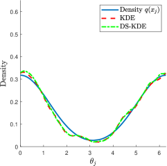
(a) Clean data

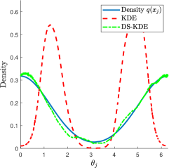
(b) Varying noise

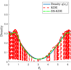
(c) Outlier-type noise

Figure 1: Example of density estimation on the unit circle using DS-KDE from (13) versus the standard KDE in clean and noisy scenarios, where $n=m=2000$, $s=2$, and $\epsilon=0.1$. The angles $\theta_{i}\in[0,2\pi)$ were sampled from $\mathcal{N}(0,0.16\pi^{2})$ modulo $2\pi$. Panel (a): Clean data. Panel (b): Heteroskedastic noise with smoothly varying magnitude; see Figure 2a. panel (c): Identically-distributed outlier type noise; see Figure 2b.

Next, we simulated two types of high-dimensional noise. First, we added noise $\eta_{i}$ sampled uniformly from a ball in $\mathbb{R}^{m}$ with radius $0.01+0.49(1+\cos(\theta_{i}))/2$, where $\theta_{i}$ is the angle of $x_{i}$ on the unit circle. Hence, the expected noise magnitude varies smoothly between $0.01$ and $0.5$ along the circle; see Figure 2a for a two-dimensional visualization. Figure 1b depicts the standard KDE as well as our robust density estimator $\hat{q}_{i}$ versus the true density $q(x_{i})$. We observe that the standard KDE produces an estimate that is very different from the true density $q(x_{i})$, and has more to do with the noise magnitudes $\|\eta_{i}\|_{2}^{2}$ in the data. On the other hand, the DS-KDE is robust to the magnitudes of the noise and produces an estimate that is nearly as accurate as in the clean case. For the second type of noise, we took each $\eta_{i}$ to be the zero vector with probability $p=0.9$ and sampled it from a multivariate normal with covariance $I_{m}/(4m)$ with probability $1-p=0.1$, thereby simulating identically-distributed outlier-type noise; see Figure 2b for a two-dimensional visualization. Figure 1c shows that in this case, the standard KDE suffers from pointwise drops in the estimated density. Essentially, these drops stem from the nonzero realizations of the noise, i.e., the “‘outliers”, whose large noise magnitudes inflate the pairwise Euclidean distances. On the other hand, the DS-KDE produces an estimate that is invariant to the outliers and is very close to $q(x_{i})$.

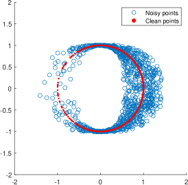
(a) Noise with smoothly varying magnitude

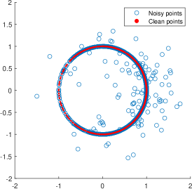
(b) Outlier type noise

Figure 2: Two-dimensional visualization of prototypical noise models used in our experiments. The clean data $x_{i}$ are sampled from the unit circle with non-uniform density as in Figure 1a. Panel (a): Heteroskedastic noise with smoothly varying magnitude, where $\eta_{i}$ is sampled uniformly from a ball in $\mathbb{R}^{m}$ with radius $0.01+0.49(1+\cos(\theta_{i}))/2$ ($\theta_{i}$ is the angle of $x_{i}$ on the unit circle). Panel (b): Identically-distributed outlier-type noise, where $\eta_{i}$ is zero with probability $0.9$ and sampled from a multivariate normal with covariance $I_{m}/(4m)$ with probability $0.1$.

It is interesting to point out that although the DS-KDE is undefined when $s=1$, the limiting case of $s\rightarrow 1$ is interpretable and can be implemented. In particular, according to (13), a direct calculation shows that

$$\lim_{s\rightarrow 1}\hat{q}_{i}=\frac{1}{n-1}\operatorname{exp}\left\{-\sum_{j=1,\;j\neq i}^{n}W_{i,j}\log(W_{i,j})\right\}.$$ (15)

The right-hand side of (15), up to the factor $1/(n-1)$, is known as the perplexity of the $i$th row of $W$, where the expression inside the exponent in (15) is the entropy. According to Theorem 3.1, we expect the right-hand side of (15) to approximate $({\pi\epsilon})^{d/2}s^{{d}/{(2(s-1))}}q(x_{i})\rightarrow(\pi e\epsilon)^{d/2}q(x_{i})$ as $s\rightarrow 1$, which provides an explicit relation between the entropy of each row of the doubly stochastic kernel $W$ and the sampled density $q(x_{i})$. We mention that Theorem 3.1 does not strictly cover the limit $s\rightarrow 1$ since the dependence of the bias and variance errors on $s$ is harder to track and is not made explicit. However, the numerical experiments described below suggest that the conclusions of Theorem 3.1 also hold for $s\rightarrow 1$, and that the performance of the density estimator in this case is comparable to other choices of $s$ over a range of bandwidth parameters $\epsilon$.

Figure 3 illustrates the maximal density estimation errors (over $i=1,\ldots,n$) for the standard KDE as well as the DS-KDE as functions of $n$, for $m=n$ and $s=0.5$, $s=2$, and $s\rightarrow 1$, where $\epsilon=0.1$. We used the same noise settings as for Figure 2, and the displayed errors were averaged over $50$ randomized trials. In the clean case, the KDE and the DS-KDE perform similarly, where all errors decrease with $n$ at a rate close to $n^{-1/2}$, which agrees with Theorem 3.1 and 8 up to a logarithmic factor. In both noisy cases, however, the KDE error saturates at a high level and does not decrease further, whereas the DS-KDE errors decrease roughly at the same rate as in the clean case. In particular, the DS-KDE errors for $n=3000$ are over an order of magnitude smaller than the standard KDE error.

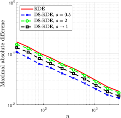
(a) Clean data

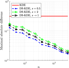
(b) Varying noise

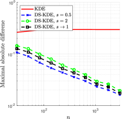
(c) Outlier-type noise

Figure 3: Density estimation errors for the standard KDE and the DS-KDE from (13) (normalized by the corresponding global constant) versus the number of samples $n$ and several values of $s$ for clean and noisy scenarios, where $m=n$. The density $q(x)$ and noise models are the same as for figures 1a, 1b, and 1c, respectively; see also figures 2a and 2b.

In Figure 4, we depict the maximal density estimation errors for the standard KDE and DS-KDE (13) as functions of $\epsilon$ for $s=0.5$, $s=2$, and $s\rightarrow 1$, where $m=n=2000$. We used the same noise settings as for Figure 2, and the displayed errors were averaged over $10$ randomized trials. We observe that in the clean case, all density estimators perform similarly well, attaining errors of about $0.02$ for the best values of $\epsilon$, with a small advantage to the DS-KDE with $s=2$. Yet, in the noisy scenarios, the standard KDE can only achieve an error of about $0.1$, which requires using a large bandwidth parameter, while the DS-KDE behaves similarly to the clean case and achieves significantly smaller errors. As expected from Theorem 3.1, we see the prototypical bias-variance trade-off in all noise scenarios, where the error of the DS-KDE is dominated by the bias term $\mathcal{O}(\epsilon)$ for large $\epsilon$, and dominated by the variance error $\max_{i}|\mathcal{E}_{i}^{(1)}|$ for small $\epsilon$. However, while the strong noise forces the standard KDE to use a large bandwidth $\epsilon$ (proportional to the magnitude of the noise) to achieve the smallest error in the bias-variance trade-off, the DS-KDE does not suffer from this issue and achieves small errors even when the bandwidth is much smaller than the noise magnitudes.

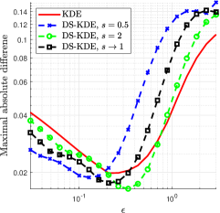
(a) Clean data

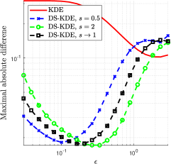
(b) Varying noise

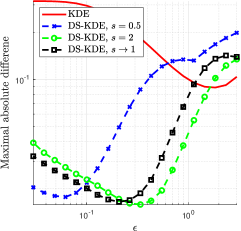
(c) Outlier-type noise

Figure 4: Density estimation errors for the standard KDE and the DS-KDE from (13) (normalized by the corresponding global constant) versus the bandwidth parameter $\epsilon$ and several values of $s$ for clean and noisy scenarios, where $m=n=2000$. The density $q(x)$ and noise models are the same as for figures 1a, 1b, and 1c, respectively; see also figures 2a and 2b.

3.2 Recovering noise magnitudes, signal magnitudes, and Euclidean distances

According to the asymptotic expression for the scaling factors $d_{i}$ in (12), we can extract the noise magnitudes $\|\eta_{i}\|_{2}^{2}$ from $d_{i}$ (up to a global constant) if we know the density $q(x_{i})$. Since we do not have access to $q(x_{i})$ directly, we replace it with its estimate $\hat{q}_{i}$ from (13) and define

$$\hat{N}_{i}=\epsilon\log\left(d_{i}\sqrt{(n-1)\hat{q}_{i}}\right),$$ (16)

for $i=1,\ldots,n$, which serves as an estimator for the noise magnitude $\|\eta_{i}\|_{2}^{2}$. In our setup of high-dimensional noise (Assumptions 2 and 3), we have $\|y_{i}\|_{2}^{2}\approx\|{x}_{i}\|_{2}^{2}+\|\eta_{i}\|_{2}^{2}$ and $\|y_{i}-y_{j}\|_{2}^{2}\approx\|x_{i}-x_{j}\|_{2}^{2}+\|\eta_{i}\|_{2}^{2}+\|\eta_{j}\|_{2}^{2}$; see Lemma A.1 and the proof of Theorem 2.1. Hence, we can infer the signal magnitudes $\|x_{i}\|_{2}^{2}$ and the pairwise Euclidean distances $\|x_{i}-x_{j}\|_{2}^{2}$ according to

$$\hat{S}_{i}=\|y_{i}\|_{2}^{2}-\hat{N}_{i},\qquad\qquad\hat{D}_{i,j}=\|y_{i}-y_{j}\|_{2}^{2}-\hat{N}_{i}-\hat{N}_{j},$$ (17)

respectively, for $i,j=1,\ldots,n$ with $j\neq i$. Equivalently, $\hat{D}_{i,j}$ from (17) can be derived directly from $W_{i,j}$ by canceling-out the term ${(q(x_{i})q(x_{j}))^{-1/2}}$ appearing in (12) via the density estimator $\hat{q}_{i}$, that is,

$$\hat{D}_{i,j}=-\epsilon\log\left\{(n-1)\sqrt{\hat{q}_{i}}W_{i,j}\sqrt{\hat{q}_{j}}\right\}.$$ (18)

Therefore, the corrected distances $\hat{D}_{i,j}$ correspond to the similarities measured by the affinity matrix $\sqrt{\hat{q}_{i}}W_{i,j}\sqrt{\hat{q}_{j}}$, which approximates the clean Gaussian kernel (up to a global constant) according to Theorem 3.1 and the results in Section 2.

We now have the following result, whose proof can be found in Appendix E.

Proposition 3.2.

Under Assumptions 1–5, there exist $\epsilon_{0},t_{0},m_{0}(\epsilon),n_{0}(\epsilon),C^{{}^{\prime}}({\epsilon})>0$, such that for all $\epsilon<\epsilon_{0}$, $m>m_{0}(\epsilon)$, $n>n_{0}(\epsilon)$, we have

$$\hat{N}_{i} =\|\eta_{i}\|_{2}^{2}+\epsilon\frac{d\log(s)}{4(s-1)}+\mathcal{O}(\epsilon^{2})+\mathcal{E}^{(2)}_{i},$$ (19)

$$\hat{S}_{i} =\|x_{i}\|_{2}^{2}-\epsilon\frac{d\log(s)}{4(s-1)}+\mathcal{O}(\epsilon^{2})+\mathcal{E}^{(3)}_{i},$$ (20)

$$\hat{D}_{i,j} =\|x_{i}-x_{j}\|_{2}^{2}-\epsilon\frac{d\log(s)}{2(s-1)}+\mathcal{O}(\epsilon^{2})+\mathcal{E}^{(4)}_{i,j},$$ (21)

for all $i,j=1,\ldots,n$, $i\neq j$, where $\max_{i}|\mathcal{E}^{(2)}_{i}|$, $\max_{i}|\mathcal{E}^{(3)}_{i}|$, and $\max_{i,j}|\mathcal{E}^{(4)}_{i,j}|$ are upper bounded by the right-hand side of (8) with probability at least $1-n^{-t}$, for any $t>t_{0}$.

Proposition 3.2 asserts that for sufficiently large $m,n$ and sufficiently small $\epsilon$, the quantities $\hat{N}_{i}$, $\hat{S}_{i}$, and $\hat{D}_{i,j}$ can approximate $\|\eta_{i}\|_{2}^{2}$, $\|x_{i}\|_{2}^{2}$, and $\|x_{i}-x_{j}\|_{2}^{2}$, respectively, up to arbitrarily small errors with high probability. According to (19), (20), and (21), the first error term in these approximations is a global constant that depends explicitly on $d$, $s$, and $\epsilon$, and thus can be removed if the intrinsic dimension $d$ is known or can be estimated. Alternatively, if one is only interested in ranking $\|\eta_{i}\|_{2}^{2}$, $\|x_{i}\|_{2}^{2}$, or $\|x_{i}-x_{j}\|_{2}^{2}$, then the relevant bias error term is improved to $\mathcal{O}(\epsilon^{2})$ since ranking is unaffected by a global additive constant. For example, this is the case if one is interested in identifying the points with the largest or smallest noise magnitudes or determining the nearest neighbors of each point $x_{i}$. The variance error terms $\mathcal{E}^{(2)}$, $\mathcal{E}^{(3)}$, $\mathcal{E}^{(4)}$ have the same behavior as $\mathcal{E}$ from Theorem 2.1 in Section 2.

Note that the noise magnitude estimator $\hat{N}_{i}$ in (16) corrects for the effect of the variability of the density $q(x_{i})$ on the scaling factors $\mathbf{d}$. However, one does not have to use $\hat{q}_{i}$ in (16), and it can be replaced with the constant $1$. In such a case, we would still have an $\mathcal{O}(\epsilon)$ bias error term in each of (19), (20), and (21), but it would depend on $q(x_{i})$ (and $q(x_{j})$ in the case of (21)). Hence, the $\mathcal{O}(\epsilon)$ term would no longer be a global constant that does not influence ranking. Consequently, the main advantage of accounting for the density is to improve the effective bias error term from $\mathcal{O}(\epsilon)$ to $\mathcal{O}(\epsilon^{2})$ under ranking.

We begin by demonstrating $\hat{N}_{i}$ and $\hat{S}_{i}$ via a toy example. We generated two centered circles in $\mathbb{R}^{2}$, one with radius $1$ and the other with radius $0.5$. We independently sampled $500$ points from the first circle and $500$ from the second circle according to the same (non-uniform) density used for Figure 1a. We then embedded all points in $\mathbb{R}^{m}$ with $m=500$ by applying a random orthogonal transformation and added i.i.d outlier-type noise $\eta_{i}$ taken to be zero with probability $0.9$ and sampled from a multivariate normal with covariance $\sigma_{i}I_{m}/m$ with probability $0.1$, where $\sigma_{i}$ is sampled uniformly from $(0,1)$; see Figure 5a for a two-dimensional visualization of this setup. Figure 5b illustrates the noisy point magnitudes $\|y_{i}\|_{2}^{2}$, where the signal magnitudes are clearly intertwined with the noise. Figure 5c illustrates the noise magnitude estimator $\hat{N}_{i}$ from (16) with $s=2$ and $\epsilon=0.1$, for each index $i=1,\ldots,1000$. It is evident that $\hat{N}_{i}$ accurately infers the true noise magnitudes $\|\eta_{i}\|_{2}^{2}$, albeit a small upward shift due to the bias term $\epsilon d\log s/(4(s-1))$ from (19). Importantly, $\hat{N}_{i}$ is invariant to the density $q(x_{i})$ and the signal magnitudes $\|x_{i}\|_{2}^{2}$. Similarly, Figure 5d shows that $\hat{S}_{i}$ accurately recovers $\|x_{i}\|_{2}^{2}$ up to a small global shift and minor fluctuations. Overall, the doubly stochastic scaling allows us to decompose $\|y_{i}\|_{2}^{2}$ into signal and noise parts. In particular, $\hat{N}_{i}$ can be utilized to identify the noisy points in this setting, while $\hat{S}_{i}$ reveals that the clean data points can be partitioned into two groups with distinct magnitudes.

(a)

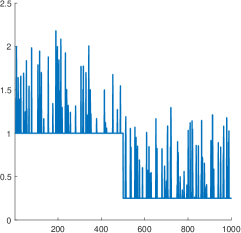
(b)

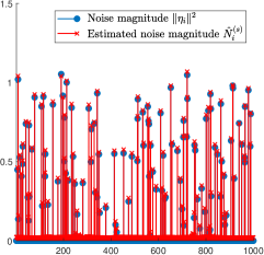
(c)

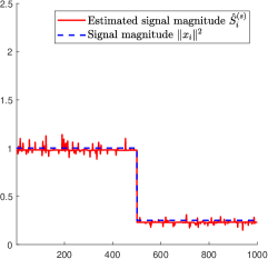
(d)

Figure 5: Example of estimating the noise magnitudes $\|\eta_{i}\|_{2}^{2}$ and signal magnitudes $\|x_{i}\|_{2}^{2}$ using $\hat{N}_{i}$ and $\hat{S}_{i}$ from (16) and (21), respectively (panels (c) and (d)), with $s=2$, $\epsilon=0.1$, for $i=1,\ldots,1000$. The noisy observations $y_{i}$ are sampled from two concentric circles, each with the non-uniform density of Figure 1a, embedded in dimension $m=500$ and corrupted with probability $0.1$ by multivariate normal noise with covariance $\sigma_{i}I_{m}$, where $\sigma_{i}$ is sampled uniformly at random from $(0,1)$ (panels (a) and (b)).

Next, we demonstrate the advantage of correcting the noisy Euclidean distances $\|y_{i}-y_{j}\|_{2}^{2}$ via $\hat{D}$ from (21). Figure 6a shows the noisy distances $\|y_{i}-y_{j}\|_{2}^{2}$ versus the clean distances $\|{x}_{i}-{x}_{j}\|_{2}^{2}$ in the setup of Figures 1b and 2a, where points are sampled from a circle and corrupted by noise with magnitude that is varying smoothly from $0.01$ to $0.5$ (see more details in the text of Section 3.1). It is evident that the Euclidean distances are strongly corrupted by the variability of the noise magnitude and deviate substantially from the desired behavior, which is the dashed diagonal line (describing perfect correspondence). In Figure 6b we depict the corrected distances $\hat{D}_{i,j}$ computed with $s=2$ and $\epsilon=0.1$, which are much closer to the clean distances and concentrate well around a line with slope $1$ that is shifted slightly below the desired trend. This shift agrees almost perfectly with the bias term $-\epsilon{d\log(s)}/{(2(s-1))}\approx-0.035$ appearing in (21). Lastly, for each $k=1,\ldots,50$, we computed the $k$ nearest neighbors of each $x_{i}$ according to the noisy distances $\|y_{i}-y_{j}\|_{2}^{2}$ and the corrected distances $\hat{D}_{i,j}$. For each $k$, Figure 6c shows the proportion of these nearest neighbors that coincide with any of the $k$ true nearest neighbors according to the clean distances $\|x_{i}-x_{j}\|_{2}^{2}$, averaged over $i=1,\ldots,1000$. It is clear that the corrected distances allow for more accurate identification of near neighbors, with more than $80\%$ accuracy for $k=50$ while the noisy distances provide less than $60\%$ accuracy in that case. Note that the nearest neighbors of each point $x_{i}$ according to the corrected distances $\hat{D}_{i,j}$ correspond to the largest entries of $\sqrt{\hat{q}_{i}}W_{i,j}\sqrt{\hat{q}_{j}}$ in each row $i$. Hence, Figure 6c also describes the advantage of the affinity matrix $\sqrt{\hat{q}_{i}}W_{i,j}\sqrt{\hat{q}_{j}}$ over the noisy Gaussian kernel ${K}_{i,j}$ in encoding similarities.

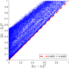
(a) Noisy vs. clean distances

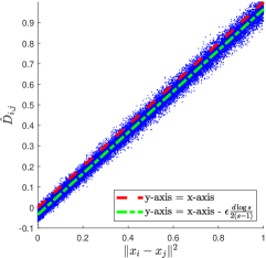
(b) Corrected vs. clean distances

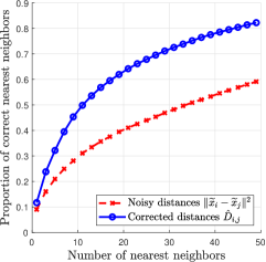
(c) Near neighbor detection

Figure 6: Influence of noise on pairwise Euclidean distances and on detection accuracy of the nearest neighbors, compared to the corrected distances $\hat{D}_{i,j}$ from (21) with $s=2$ and $\epsilon=0.1$. The data is sampled from a unit circle with non-uniform density, embedded in dimension $m=1000$ and corrupted by noise whose magnitude varies smoothly from $0.01$ to $0.5$; see Figures 1b and 2a and relevant text.

3.3 Robust weighted manifold Laplacian approximation

In what follows we construct a family of normalizations that is a robust analogue of (2) and establish convergence to the associated family of differential operators (see [17]).

Fix $\alpha\in[0,1]$, and define

$$L^{(\alpha)}=\frac{4(I_{n}-\hat{W}^{(\alpha)})}{\epsilon},\qquad\hat{W}^{(\alpha)}_{i,j}=\frac{\widetilde{W}^{(\alpha)}_{i,j}}{\sum_{j=1}^{n}\widetilde{W}^{(\alpha)}_{i,j}},\qquad\widetilde{W}^{(\alpha)}_{i,j}=\frac{W_{i,j}}{\left[\hat{q}_{i}\hat{q}_{j}\right]^{\alpha-1/2}},$$ (22)

for all $i,j=1,\ldots,n$, where $I_{n}$ is the $n\times n$ identity matrix, and $L^{(\alpha)}$ is an appropriately-normalized graph Laplacian for $\hat{W}^{(\alpha)}$. The formulas in (22) are equivalent to those in (2) except that we utilize the robust density estimator $\hat{q}_{i}$ instead of the standard KDE and further account for the asymptotic approximation of $W$ in 12 (leading to the power $\alpha-0.5$ in the denominator of $\widetilde{W}^{(\alpha)}$ instead of the power $\alpha$ appearing in $P^{(\alpha)}$ of (2)). Note that when $\alpha=0.5$, no normalization of $W$ is actually performed since $\hat{W}^{(0.5)}_{i,j}=W_{i,j}$.

Next, we define the Schrodinger-type differential operator

$$\{T^{(\alpha)}f\}(x)=\frac{\Delta_{\mathcal{M}}\{fq^{1-\alpha}\}(x)}{[q(x)]^{1-\alpha}}-\frac{\Delta_{\mathcal{M}}\{q^{1-\alpha}\}(x)}{[q(x)]^{1-\alpha}}f(x),$$ (23)

for any $f\in\mathcal{C}^{2}(\mathcal{M})$, where $\Delta_{\mathcal{M}}$ is the negative Laplace-Beltrami operator on $\mathcal{M}$. If the sampling density is uniform, i.e., $q(x)$ is a constant function, then $T^{(\alpha)}$ reduces to $\Delta_{\mathcal{M}}$ for any $\alpha$. Otherwise, $T^{(\alpha)}$ depends on the density $q(x)$, except for the special case of $\alpha=1$, where the density vanishes and $T^{(\alpha)}$ again becomes $\Delta_{\mathcal{M}}$. When $\alpha=0.5$, $T^{(\alpha)}$ is the Fokker-Planck operator describing Brownian motion via the Langevin equation [53], and when $\alpha=0$, $T^{(\alpha)}$ describes the limiting operator of the popular random walk graph Laplacian.

We now have the following result, whose proof can be found in Appendix F.

Theorem 3.3.

Fix $f\in\mathcal{C}^{3}(\mathcal{M})$. Under Assumptions 1–5, there exist $\epsilon_{0},t_{0},m_{0}(\epsilon),n_{0}(\epsilon),C^{{}^{\prime}}({\epsilon})>0$, such that for all $\epsilon<\epsilon_{0}$, $m>m_{0}(\epsilon)$, $n>n_{0}(\epsilon)$, we have

$$\sum_{j=1}^{n}L^{(\alpha)}_{i,j}f(x_{j})=\{T^{(\alpha)}f\}(x_{i})+\mathcal{O}(\epsilon^{\beta})+\mathcal{E}^{(5)}_{i},$$ (24)

for all $i=1,\ldots,n$, where $\max_{i}|\mathcal{E}_{i}^{(5)}|$ is upper bounded by the right-hand side of (8) with probability at least $1-n^{-t}$, for any $t>t_{0}$.

Theorem 3.3 shows that for sufficiently large $m,n$, and sufficiently small $\epsilon$, the matrix $L^{(\alpha)}$ can approximate the action of the operator $T^{(\alpha)}$ pointwise up to an arbitrarily small error with high probability. If $\alpha=1$, then $L^{(\alpha)}$ approximates the (negative) Laplace-Beltrami operator $\Delta_{\mathcal{M}}$, which encodes the intrinsic geometry of the manifold [17] regardless of the sampling density. If $\alpha=0.5$, then $L^{(\alpha)}=4(I_{n}-W)/\epsilon$ approximates the Fokker-Planck operator, suggesting that the doubly stochastic Markov matrix $W$ simulates Langevin diffusion on $\mathcal{M}$, agreeing with the results in [50, 80, 14]. If $\alpha=0$, we have $\widetilde{W}^{(\alpha)}_{i,j}=\sqrt{\hat{q}_{i}}W_{i,j}\sqrt{\hat{q}_{j}}$, which corrects for the influence of density on $W$ according to (12), approximating the clean Gaussian kernel up to a global constant. In this case, $L^{(\alpha)}$ approximates the same operator as the standard random walk graph Laplacian on the clean data. Theorem 3.3 shows that the popular family of normalizations (2) can be made robust to general high-dimensional noise via the doubly stochastic affinity matrix $W$ and our robust density estimator (13).

In Figure 7 we demonstrate the advantage of the robust graph Laplacian normalization (22) for $\alpha=1$ over the traditional normalization $4(I_{n}-\hat{P}^{(1)})/\epsilon$, where $\hat{P}^{(1)}$ is from (2). We used the same setting as the one used for Figure 1a and Figure 1b, namely the unit circle with non-uniform density, where the sampled points are either clean or corrupted by smoothly varying noise; see more details in the corresponding text of Section 3.1. To quantify the accuracy of the approximation in (24), we used the test function $f(\theta(x))=(\cos(\theta(x))+\sin(2\theta(x)))/5$, where $\theta(x)\in[0,2\pi)$ is the angle of a point $x$ on the circle. For $\alpha=1$, $T^{(\alpha)}$ reduces to the Laplace-Beltrami operator $\Delta_{\mathcal{M}}$, in which case $\{\Delta_{\mathcal{M}}(f)\}(x_{i})=(-\cos(\theta_{i})-4\sin(2\theta_{i}))/5$, where $\theta_{i}=\theta(x_{i})$. We then computed the maximal absolute difference between $\sum_{j=1}^{n}L^{(\alpha)}_{i,j}f(x_{j})$ and $\{\Delta_{\mathcal{M}}(f)\}(x_{i})$ over $i=1,\ldots,n$, both for our robust normalization as well as the traditional one. Figure 7a shows these errors versus the sample size $n$, where $\epsilon=0.1$, $s=2$, $m=n$, and we averaged the errors over $30$ randomized trials. Figure 7a shows the same errors versus the bandwidth parameter $\epsilon$, where $m=n=5000$, $s=2$, and we averaged the results over $20$ randomized trials. It is evident that the robust and the traditional graph Laplacian normalizations perform nearly identically in the clean case, both across $n$ and across $\epsilon$, suggesting that the bias and variance errors in (24) match those for the traditional normalization, at least in our setting. On the other hand, the robust normalization performs much better in the noisy case whenever the error is dominated by the variance term, i.e., when $\epsilon$ is sufficiently small with respect to the sample size $n$, while having almost identical behavior when the error is dominated by the bias term. Consequently, the robust normalization achieves smaller errors for any fixed bandwidth in this scenario, and allows us to use a smaller optimally-tuned bandwidth to obtain a better approximation of the Laplace-Beltrami operator under noise.

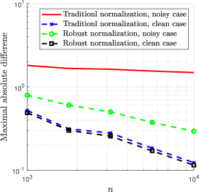
(a) Error versus $n$

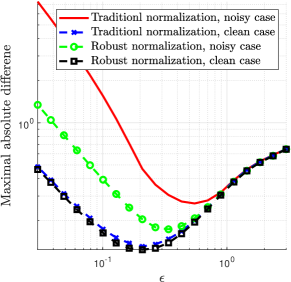
(b) Error versus $\epsilon$

Figure 7: Maximal absolute difference between the Laplace-Beltrami operator $\{\Delta_{\mathcal{M}}f\}(x_{i})$ and its approximation $\sum_{j=1}^{n}L^{(\alpha)}_{i,j}f(x_{j})$ using the robust graph Laplacian normalization (22) with $\alpha=1$ and its traditional counterpart, versus the sample size $n$ and the bandwidth $\epsilon$. The data is sampled according to the setting used for Figures 1a,  1b, and 2a, namely a unit circle with non-uniform density where the points are either clean or corrupted by smoothly varying noise in high dimension.

4 Experiments on real single-cell RNA-sequencing data

In this section, we demonstrate our results using real data from Single-cell RNA-sequencing (scRNA-seq), which is a revolutionary technology for measuring high-dimensional gene expression profiles of individual cells in diverse populations [72, 48]. In this case, each observation $\widetilde{y}_{i}\in\mathbb{R}^{m}$ is a vector of nonnegative integers describing the expression levels of $m$ different genes in the $i$’th cell of the sample. The high resolution of the data – given at the single-cell level – makes it possible to study the similarities between different cells and to characterize different cell populations, which is of paramount importance in immunology and developmental biology. However, one of the main challenges in analyzing scRNA-seq data is the high levels of noise and its non-uniform nature [38, 39, 40].

To demonstrate our results, we used the popular dataset of Purified Peripheral Blood Mononuclear Cells (PBMC) by [85], where $32733$ genes are sequenced over $94654$ cells that are annotated experimentally according to $10$ known cell types. To preprocess the data, we first randomly subsampled $500$ cells from each of the following types: ‘b cells’, ‘cd14 monocytes’, ‘cd34’, ‘cd4 helper’, ‘cd56 nk’, and ‘cytotoxic t’. These cell types are fairly distinguishable one from another, thereby simplifying the interpretability of our subsequent results, while the subsampling makes computations more tractable. We then computed the total expression count for each cell, given by $c_{i}=\sum_{j=1}^{m}\widetilde{y}_{i,j}$, where $\widetilde{y}_{i,j}$ denotes the $j$’th entry of $\widetilde{y}_{i}$, and computed the normalized observations $y_{i}=\widetilde{y}_{i}/c_{i}$. This is a standard normalization in scRNA-seq for making the cell descriptors to be probability vectors, thereby removing the influence of technical variability of counts (also known as “read depth”) across cell populations [76, 20]. The doubly stochastic scaling of the Gaussian kernel is then evaluated using the normalized observations $y_{1},\ldots,y_{n}$, $n=3000$, with a prescribed tolerance of $10^{-6}$ and a maximum of $10^{4}$ iterations in the algorithm of [80].

In our first experiment, we set out to investigate the accuracy of noise magnitude estimator $\hat{N}_{i}$ described in (16). To validate our noise estimates, we assume the popular Poisson data model $\widetilde{y}_{i,j}\sim\operatorname{Poisson}(\mu_{i,j})$ [61]. In this case, we have $\mathbb{E}[\widetilde{y}_{i,j}]=\operatorname{Var}[\widetilde{y}_{i,j}]=\mu_{i,j}$, and by standard concentration arguments,

$$\|\eta_{i}\|_{2}^{2}\sim\frac{\sum_{j=1}^{m}\left(\widetilde{y}_{i,j}-\mu_{i,j}\right)^{2}}{c_{i}^{2}}\sim\frac{\sum_{j=1}^{m}\operatorname{Var}[\widetilde{y}_{i,j}]}{c_{i}^{2}}=\frac{\sum_{j=1}^{m}\mu_{i,j}}{c_{i}^{2}}\sim\frac{\sum_{j=1}^{m}\widetilde{y}_{i,j}}{c_{i}^{2}}=\frac{1}{c_{i}},$$ (25)

asymptotically as $m\rightarrow\infty$ under appropriate de-localization conditions on the Poisson parameters $\{\mu_{i,j}\}_{j=1}^{m}$. Therefore, we expect the noise magnitude $\|\eta_{i}\|_{2}^{2}$ to be close to $1/c_{i}$, which is the inverse of the total gene expression counts for cell $i$. Figure 8a depicts the estimated noise magnitudes $\hat{N}_{i}$ computed with $\epsilon=2\cdot 10^{-5}$ and $s=2$, versus $1/c_{i}$ for a prototypical subsampled dataset (with $3000$ cells total, $500$ from each of six different types). Evidently, the Poisson model suggests that the noise magnitude fluctuates considerably across the data, roughly by an order of magnitude. Of course, the noise magnitude estimator $\hat{N}_{i}$ is completely oblivious to the Poisson model and does not have access to the total counts $c_{i}$ (as it is determined solely from the normalized observations). Nonetheless, the estimated noise magnitudes $\hat{N}_{i}$ concentrate around the red dashed diagonal line, showcasing good agreement with the Poisson model. Note that there seems to be a slight quadratic trend to the estimated noise magnitudes, which is in line with literature suggesting over-dispersion with respect to the standard Poisson [70] (e.g., negative binomial).

In our second experiment, we employ the cell type annotations to assess the accuracy of $\hat{W}_{i,j}^{(\alpha)}$ from (22) and its traditional counterpart $\hat{P}^{(\alpha)}$ from (2). Since $\hat{W}_{i,j}^{(\alpha)}$ is a transition probability matrix, it describes a random walk over the cells. It is reasonable to assume that a random walk that starts at a certain cell should be unlikely to immediately transition to a cell with a different type. Motivated by this reasoning, we show in Figure 8b the probability of a cell to transition to a cell with a different type, averaged over all cells $i=1,\ldots,3000$, according to $\hat{W}_{i,j}^{\alpha}$ from (22) as well as is traditional counterpart, where we used $s=2$, $\alpha=0,0.5,1$, and averaged the results over $20$ randomized trials (of subsampling cells), plotted against the bandwidth parameter $\epsilon$. Figure 8c is the same as Figure 8b except that we averaged the aforementioned probabilities over the cells in each cell type separately and took the largest of these, namely the worst-case averaged transition probability over the six cell types.

From Figures 8b and 8c it is evident that for large bandwidth parameters $\epsilon$, all normalizations provide similarly undesirable behavior in the form of large probabilities of transition errors, namely probabilities to transition between different cell types. As we decrease $\epsilon$, the behavior generally improves across all normalizations, but the errors made by the robust normalizations $\hat{W}^{(\alpha)}$ are consistently smaller than the traditional ones. This advantage of our normalizations is particularly evident over the traditional normalization with $\alpha=0$, whose worst-case error (for one of the cell types) exceeds $0.4$ for all values of $\epsilon$. The traditional normalization with $\alpha=0.5$ seems to be more accurate than $\alpha=0$ or $\alpha=1$ and provides results very similar to the robust normalizations, albeit slightly larger worst-case errors for small $\epsilon$. Recall that the traditional normalization with $\alpha=0.5$ is obtained by first performing the symmetric normalization $D_{i}^{-1/2}W_{i,j}D_{i}^{-1/2}$, where $D_{i}=\sum_{j=1}^{n}{K}_{i,j}$, and then performing a row-stochastic normalization. These steps are precisely one iteration of the accelerated scaling algorithm described in [80], which can possibly explain the advantage of $\alpha=0.5$ over the other values of $\alpha$.

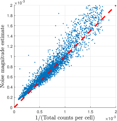
(a) Estimated noise vs. Poisson noise

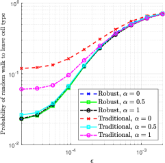
(b) Average transition probability error

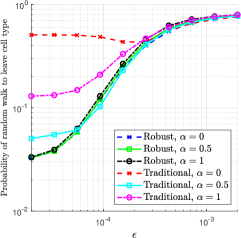
(c) Worst-case transition probability error

Figure 8: Accuracy of the noise magnitude estimate $\hat{N}_{i}$ from (16) (panel (a)) and the Markov matrix $\hat{W}^{(\alpha)}$ from (22) as well as its traditional analogue $\hat{P}^{(\alpha)}$ from (2) (panels (b) and (c)), evaluated using the annotated single-cell RNA-sequencing data from [85]. The noise magnitude estimate $\hat{N}_{i}$ is compared to the anticipated value from the Poisson model (25), while the error in the Markov matrix $\hat{W}^{(\alpha)}$ and its traditional analogue is assessed by the average probability to transition between distinct cell types (the smaller the better), plotted against the bandwidth parameter $\epsilon$.

Note that all robust normalizations provide nearly identical probabilities of transition errors, which may initially seem strange in light of the different limiting operators for the corresponding graph Laplacians in Theorem 3.3. However, an important distinction is that the graph Laplacian $L^{(\alpha)}$ only describes the first-order behavior $W^{(\alpha)}$ in $\epsilon$, while its zeroth-order behavior is given by $\sum_{j=1}^{n}\hat{W}^{(\alpha)}_{i,j}f(x_{j})\sim f(x_{i})$ for large $m,n$ and small $\epsilon$, regardless of $\alpha$. Hence, we should indeed expect the random walk transition probability errors to be very similar across $\alpha$, which is the case for the robust normalization. On the other hand, the random walk transition probability errors for the traditional normalization differ substantially across $\alpha$, which is likely due to the strong variability of the noise in the data (see Figure 8a) and the sensitivity of the standard kernel density estimator to such noise.

5 Discussion

The results in this work give rise to several future research directions. On the practical side, to make the tools we developed in Section 3 widely applicable, it is desirable to derive procedures for adaptively tuning the bandwidth parameter $\epsilon$ and the parameter $s$ in the DS-KDE (13). Moreover, for large experimental datasets, the density can vary considerably across the sample space, where a global bandwidth parameter is unlikely to provide a satisfactory bias-variance trade-off. Hence, it is worthwhile to tune the bandwidth according to the local density around each point. Techniques for adaptive bandwidth selection have been extensively studied for standard kernel density estimation and traditional graph Laplacian normalizations in the clean case (see [84, 7] and references therein), e.g., by near neighbor distances. However, the adaptation of these techniques to our setting is nontrivial, as the near-neighbor distances could be too corrupted for determining the local bandwidth. Therefore, this topic requires substantial analytical and empirical investigation that is left for future work.

On the theoretical side, one important direction is to characterize the constant $C^{{}^{\prime}}(\epsilon)$ appearing in (8) in terms of $\epsilon$. This would require a more advanced analysis of the stability of the scaling factors $\mathbf{d}$ under perturbations in ${W}$ and the prescribed row sums, which is beyond the scope of this work. In addition, we conjecture that the results in Theorem 2.2 can be strengthened, and specifically that $\rho_{\epsilon}(x)=q^{-1/2}(x)F_{\epsilon}(x)+\mathcal{O}(\epsilon^{2})$ uniformly over $x\in\mathcal{M}$. Currently, Theorem 2.2 only proves an analogous $L^{p}$ bound for $p\in[1,4/3)$, while the pointwise bound in Theorem 2.2 is only for $d\leq 5$ and is dominated by a dimension-dependent error that is worse than $\mathcal{O}(\epsilon^{2})$. A useful first step in that direction might be to obtain a tighter characterization of $\rho_{\epsilon}$ than in our Lemma A.3. However, this will require different theoretical tools and is left for future work. Lastly, properly refined versions of Theorems 2.1 and 2.2 can be combined to describe how to tune the bandwidth parameter $\epsilon$ for convergence of the approximation errors described in Sections 3.1 and 3.3.

Appendix A Supporting lemmas

A.1 Concentration of inner products

Lemma A.1.

Under Assumptions 1 and 2, there exist universal constants $c,m_{0},t_{0}>0$, such that for any $t>t_{0},m>m_{0}$, and $i\neq j$ we have

$$\operatorname{Pr}\left\{\left|\langle y_{i},y_{j}\rangle-\langle{x}_{i},{x}_{j}\rangle\right|>ct\sqrt{\log m}\cdot\operatorname{max}\{E,E^{2}\sqrt{m}\}\right\}\leq m^{-t}.$$ (26)

Proof.

Let us write

$$\langle y_{i},y_{j}\rangle=\langle{x}_{i},{x}_{j}\rangle+\langle{\eta}_{i},{x}_{j}\rangle+\langle{x}_{i},\eta_{j}\rangle+\langle\eta_{i},\eta_{j}\rangle.$$ (27)

Conditioning on $x_{1},\ldots,x_{n}$, the random variable $\langle{\eta}_{i},{x}_{j}\rangle$, for each $i=1,\ldots,n$, is sub-Gaussian with

$$\|\langle{\eta}_{i},{x}_{j}\rangle\|_{\psi_{2}}\leq\|x_{j}\|_{2}\sup_{\|y\|_{2}=1}\|\langle{\eta}_{i},y\rangle\|_{\psi_{2}}\leq E,$$ (28)

where we also used the definition of sub-Gaussian norm [75] and the fact that $\|x_{i}\|_{2}\leq 1$. Therefore, according to Proposition 2.5.2 in [75], we have

$$\operatorname{Pr}\{|\langle{\eta}_{i},{x}_{j}\rangle|>\tau\}\leq 2\operatorname{exp}\left\{-\frac{\tau^{2}}{c^{2}\|\langle{\eta}_{i},{x}_{j}\rangle\|_{\psi_{2}}^{2}}\right\}\leq 2\operatorname{exp}\left\{-\frac{\tau^{2}}{c^{2}E^{2}}\right\},$$ (29)

where $c$ is a universal constant. Taking $\tau=cE\sqrt{t\log m}$, for any $t>0$, shows that

$$\operatorname{Pr}\{|\langle{\eta}_{i},{x}_{j}\rangle|>cE\sqrt{t\log m}\}\leq 2m^{-t}.$$ (30)

Analogously, the above holds when replacing $\langle{\eta}_{i},{x}_{j}\rangle$ with $\langle{x}_{i},\eta_{j}\rangle$. Since (30) holds conditionally on any realization of $x_{1},\ldots,x_{n}$, it also holds unconditionally. Next, conditioning on $\eta_{i}$ for any $i\in\{1,\ldots,n\}$, the random variable $\langle\eta_{i},\eta_{j}\rangle$ for $j\neq i$ is also sub-Gaussian, where

$$\bigg{\|}\left(\langle\eta_{i},\eta_{j}\rangle\;\bigg{|}\;\eta_{i}=h\right)\bigg{\|}_{\psi_{2}}\leq\|h\|_{2}\sup_{\|y\|_{2}=1}\|\langle y,{\eta}_{j}\rangle\|_{\psi_{2}}\leq{E\|h\|_{2}}.$$ (31)

Hence, by the definition of a sub-Gaussian random variable

$$\operatorname{Pr}\left\{|\langle{\eta}_{i},{\eta}_{j}\rangle|>\tau\;\bigg{|}\;\|\eta_{i}\|_{2}\leq r\right\}\leq 2\operatorname{exp}\left\{-\frac{\tau^{2}}{c^{2}\bigg{\|}\left(\langle{\eta}_{i},\eta_{j}\rangle\;\bigg{|}\;\|\eta_{i}\|_{2}\leq r\right)\bigg{\|}_{\psi_{2}}^{2}}\right\}\leq 2\operatorname{exp}\left\{-\frac{\tau^{2}}{c^{2}E^{2}r^{2}}\right\},$$ (32)

and taking $\tau=crE\sqrt{t\log m}$, for any $t>0$, gives

$$\operatorname{Pr}\left\{|\langle{\eta}_{i},{\eta}_{j}\rangle|>crE\sqrt{{t\log m}}\;\bigg{|}\;\|\eta_{i}\|_{2}\leq r\right\}\leq 2m^{-t}.$$ (33)

We can now write

$$\operatorname{Pr}\left\{|\langle{\eta}_{i},{\eta}_{j}\rangle|>crE\sqrt{{t\log m}}\right\} =\operatorname{Pr}\left\{|\langle{\eta}_{i},{\eta}_{j}\rangle|>crE\sqrt{{t\log m}}\;\bigg{|}\;\|\eta_{i}\|_{2}\leq r\right\}\operatorname{Pr}\{\|\eta_{i}\|_{2}\leq r\}$$

$$+\operatorname{Pr}\left\{|\langle{\eta}_{i},{\eta}_{j}\rangle|>crE\sqrt{{t\log m}}\;\bigg{|}\;\|\eta_{i}\|_{2}>r\right\}\operatorname{Pr}\{\|\eta_{i}\|_{2}>r\}$$

$$\leq 2m^{-t}+\operatorname{Pr}\{\|\eta_{i}\|_{2}>r\}.$$ (34)

Therefore, we need a probabilistic bound on $\|\eta_{i}\|_{2}$. Applying Theorem 2.1 in [34] to the sub-Gaussian random vector $\eta_{i}$ tells us that

$$\operatorname{Pr}\left\{\|\eta_{i}\|_{2}>\|\eta_{i}\|_{\psi_{2}}\left(c_{1}\sqrt{m}+c_{2}\sqrt{\log(1/\delta)}\right)\right\}\leq\delta,$$ (35)

for any $\delta\in(0,1)$, where $c_{1},c_{2}>0$ are universal constants. Taking $\delta=m^{-t}$ and letting $r=E({c_{1}\sqrt{m}}+c_{2}\sqrt{t\log m})$, we arrive at

$$\operatorname{Pr}\left\{|\langle{\eta}_{i},{\eta}_{j}\rangle|>cE^{2}\sqrt{{t\log m}}\left({c_{1}\sqrt{m}}+c_{2}\sqrt{{t\log m}}\right)\right\}\leq 3m^{-t},$$ (36)

for any $t>0$. Combining (36), (30), (27), and applying the union bound, provides the required result. ∎

A.2 Stability of scaling factors

Lemma A.2.

Let ${A}\in\mathbb{R}^{n\times n}$, $n\geq 3$, be a symmetric nonnegative matrix with zero main diagonal and strictly positive off-diagonal entries. Denote by $\mathbf{v}=[v_{1},\ldots,v_{n}]>0$ the unique vector for which $D(\mathbf{v})AD(\mathbf{v})$ is doubly stochastic, and suppose that there exist $\varepsilon\in(0,1)$ and a vector $\hat{\mathbf{v}}=[\hat{v}_{1},\ldots,\hat{v}_{n}]>0$ such that

$$\left|\sum_{j=1}^{n}\hat{v}_{i}{A}_{i,j}\hat{v}_{j}-1\right|\leq\varepsilon,$$ (37)

for all $i=1,\ldots,n$. Then,

$$\sqrt{\frac{1-\delta}{1+\varepsilon}}\leq\frac{{v}_{i}}{\hat{v}_{i}}\leq\sqrt{\frac{1}{(1-\delta)(1-\varepsilon)}},$$ (38)

for all $i=1,\ldots,n$, where

$$\delta=\min\left\{1,\frac{4\varepsilon}{(n-2)\min_{i,j=1,\ldots,n,i\neq j}\left\{\hat{v}_{i}A_{i,j}\hat{v}_{j}\right\}}\right\}.$$ (39)

Proof.

Let us define

$$P_{i,j}=v_{i}A_{i,j}v_{j},\qquad\hat{P}_{i,j}=\hat{v}_{i}A_{i,j}\hat{v}_{j},\qquad u_{i}=\frac{{v}_{i}}{\hat{v}_{i}},\qquad\ell=\operatorname{argmin}_{i}u_{i},\qquad k=\operatorname{argmax}_{i}u_{i}.$$ (40)

Using (37) we can write

$$1=\sum_{j=1}^{N}{P}_{\ell,j}=\sum_{j=1}^{N}u_{\ell}\hat{P}_{\ell,j}u_{j}\leq\min_{i}u_{i}\max_{i}u_{i}\sum_{j=1}^{N}\hat{P}_{\ell,j}\leq(1+\varepsilon)\min_{i}u_{i}\max_{i}u_{i}.$$ (41)

Similarly, we have

$$1=\sum_{j=1}^{N}{P}_{k,j}=\sum_{j=1}^{N}u_{k}\hat{P}_{k,j}u_{j}\geq\max_{i}u_{i}\min_{i}u_{i}\sum_{j=1}^{N}\hat{P}_{k,j}\geq(1-\varepsilon)\max_{i}u_{i}\min_{i}u_{i}.$$ (42)

Combining (41) and (42), we obtain

$$\frac{1}{1+\varepsilon}\leq\max_{i}u_{i}\min_{i}u_{i}\leq\frac{1}{1-\varepsilon}.$$ (43)

Continuing, employing (43) and the fact that $u_{k}=\max_{i}u_{i}$, we can write

$$1=\sum_{j=1}^{n}{P}_{k,j}=\sum_{j=1}^{n}u_{k}\hat{P}_{k,j}u_{j}\geq\frac{1}{(1+\varepsilon)}\sum_{j=1}^{n}\hat{P}_{k,j}\frac{u_{j}}{\min_{i}u_{i}},$$ (44)

implying that

$$\sum_{j=1}^{n}\hat{P}_{k,j}\left(\frac{u_{j}}{\min_{i}u_{i}}-1\right)\leq{1+\varepsilon}-\sum_{j=1}^{n}\hat{P}_{k,j}\leq{2\varepsilon}.$$ (45)

Multiplying (45) by $\min_{i}u_{i}/\min_{j\neq k}\hat{P}_{k,j}$ and using the fact that $\hat{P}_{k,k}=0$, it follows that

$$\sum_{j=1,\;j\neq k}^{n}({u_{j}}-\min_{i}u_{i})\leq\sum_{j=1}^{n}\frac{\hat{P}_{k,j}}{\min_{j\neq k}\hat{P}_{k,j}}({u_{j}}-\min_{i}u_{i})\leq\frac{2\varepsilon\min_{i}u_{i}}{\min_{j\neq k}\hat{P}_{k,j}}\leq\frac{2\varepsilon\max_{i}u_{i}}{\min_{j\neq k}\hat{P}_{k,j}}.$$ (46)

We next provide a derivation analogous to (44)–(46) to obtain a bound for $\sum_{j=1,\;j\neq\ell}^{n}(\max_{i}u_{i}-u_{j})$. Using (43) and the fact that $u_{\ell}=\min_{i}u_{i}$, we can write

$$1=\sum_{j=1}^{n}{P}_{\ell,j}=\sum_{j=1}^{n}u_{\ell}\hat{P}_{\ell,j}u_{j}\leq\frac{1}{(1-\varepsilon)}\sum_{j=1}^{n}\hat{P}_{\ell,j}\frac{u_{j}}{\max_{i}u_{i}},$$ (47)

implying that

$$\sum_{j=1}^{n}\hat{P}_{\ell,j}\left(\frac{u_{j}}{\max_{i}u_{i}}-1\right)\geq{1-\varepsilon}-\sum_{j=1}^{n}\hat{P}_{\ell,j}\geq{-2\varepsilon}.$$ (48)

Multiplying the above by $-\max_{i}u_{i}/\min_{j\neq\ell}\hat{P}_{\ell,j}$ and using the fact that $\hat{P}_{\ell,\ell}=0$, it follows that

$$\sum_{j=1,\;j\neq\ell}^{n}(\max_{i}u_{i}-{u_{j}})\leq\sum_{j=1}^{n}\frac{\hat{P}_{\ell,j}}{\min_{j\neq\ell}\hat{P}_{\ell,j}}(\max_{i}u_{i}-{u_{j}})\leq\frac{2\varepsilon\max_{i}u_{i}}{\min_{j\neq\ell}\hat{P}_{\ell,j}}.$$ (49)

Next, summing (46) and (49) gives

$$(n-2)\left(\max_{i}u_{i}-\min_{i}u_{i}\right)\leq\frac{4\varepsilon\max_{i}u_{i}}{\min_{i\neq j}\hat{P}_{i,j}},$$ (50)

while it is also clear that

$$(n-2)\left(\max_{i}u_{i}-\min_{i}u_{i}\right)\leq(n-2)\max_{i}u_{i},$$ (51)

since $\min_{i}u_{i}>0$. Therefore, we have

$$0\leq 1-\frac{\min_{i}u_{i}}{\max_{i}u_{i}}\leq\delta,$$ (52)

or equivalently,

$$1-\delta\leq\frac{\min_{i}u_{i}}{\max_{i}u_{i}}\leq 1,$$ (53)

where $\delta$ is from (39). Finally, combining (53) with (43), after some manipulation tells us that

$$\sqrt{\frac{1-\delta}{1+\varepsilon}}\leq\min_{i}u_{i}\leq u_{j}\leq\max_{i}u_{i}\leq\sqrt{\frac{1}{(1-\delta)(1-\varepsilon)}},$$ (54)

for all $j=1,\ldots,n$. ∎

A.3 Boundedness of the scaling function $\rho_{\epsilon}(x)$

Lemma A.3.

Under assumption 1, there exist constants $\epsilon_{0},C>0$ that depend only on $\mathcal{M}$ and $q$, such that $|\{x\in\mathcal{M}:\;\rho_{\epsilon}(x)>t\}|\leq C/t^{2}$ for all $\epsilon\leq\epsilon_{0}$ and $t>0$.

Proof.

Let $\Omega_{\epsilon}^{t}:=\{x\in\mathcal{M}:\;\rho_{\epsilon}(x)>t\}$. For any $x\in\Omega_{\epsilon}^{t}$, we can write

$$\frac{1}{t} >\frac{1}{\rho_{\epsilon}(x)}=\frac{1}{(\pi\epsilon)^{d/2}}\int_{\mathcal{M}}\mathcal{K}_{\epsilon}(x,y)\rho_{\epsilon}(y)q(y)d\mu(y)\geq\frac{1}{(\pi\epsilon)^{d/2}}\int_{\Omega_{\epsilon}^{t}}\mathcal{K}_{\epsilon}(x,y)\rho_{\epsilon}(y)q(y)d\mu(y)$$

$$\geq\frac{ct}{(\pi\epsilon)^{d/2}}\int_{\Omega_{\epsilon}^{t}}\mathcal{K}_{\epsilon}(x,y)d\mu(y),$$ (55)

where $c:=\min_{x\in\mathcal{M}}q(x)>0$ by the positivity and continuity of $q(x)$. Next, let $B_{r}(x)$ be a ball in $\mathbb{R}^{m}$ of radius $r$ and center $x\in\mathbb{R}^{m}$, and consider a sequence of points $x_{1}^{{}^{\prime}},\ldots,x_{\kappa_{\epsilon}^{t}}^{{}^{\prime}}\in\Omega_{\epsilon}^{t}$ such that the balls $\{B_{\sqrt{\epsilon}}(x_{i}^{{}^{\prime}})\}$ are disjoint. We take $\kappa_{\epsilon}^{t}$ to be the largest integer that allows for this property, noting that such a maximum exists since $\Omega_{\epsilon}^{t}\subseteq\mathcal{M}\subset B_{1}(0)$. Then, $\cup_{i=1}^{\kappa_{\epsilon}^{t}}B_{2\sqrt{\epsilon}}(x_{i}^{{}^{\prime}})$ is a covering of $\Omega_{\epsilon}^{t}$, as otherwise it would be a contradiction to maximality of $\kappa_{\epsilon}^{t}$. We have

$$|\Omega_{\epsilon}^{t}| =\int_{\Omega_{\epsilon}^{t}}d\mu(y)\leq\sum_{i=1}^{\kappa_{\epsilon}^{t}}\int_{\Omega_{\epsilon}^{t}\cap B_{2\sqrt{\epsilon}}(x_{i}^{{}^{\prime}})}d\mu(y)\leq e^{4}\sum_{i=1}^{\kappa_{\epsilon}^{t}}\int_{\Omega_{\epsilon}^{t}\cap B_{2\sqrt{\epsilon}}(x_{i}^{{}^{\prime}})}\mathcal{K}_{\epsilon}(x,y)d\mu(y)$$

$$\leq e^{4}\sum_{i=1}^{\kappa_{\epsilon}^{t}}\int_{\Omega_{\epsilon}^{t}}\mathcal{K}_{\epsilon}(x,y)d\mu(y)\leq\frac{e^{4}(\pi\epsilon)^{d/2}}{ct^{2}}\kappa_{\epsilon}^{t},$$ (56)

where we used (55) in the last inequality. Let $\overline{\kappa}_{\epsilon}$ be the largest integer for which there is a sequence of points $\overline{x}_{1},\ldots,\overline{x}_{\overline{\kappa}_{\epsilon}}\in\mathcal{M}$ such that $\{B_{\sqrt{\epsilon}}(\overline{x}_{i})\}$ are disjoint. Certainly, we have $\kappa_{\epsilon}^{t}\leq\overline{\kappa}_{\epsilon}$. Since $\mathcal{M}$ is a smooth and compact Riemannian manifold with no boundary and intrinsic dimension $d$, there exist constants $\overline{c},\epsilon_{0}>0$ that depend only on $\mathcal{M}$, such that

$$\kappa_{\epsilon}^{t}\leq\overline{\kappa}_{\epsilon}\leq\frac{|\mathcal{M}|}{\min_{x\in\mathcal{M}}|\mathcal{M}\cap B_{\sqrt{\epsilon}}(x)|}\leq\frac{|\mathcal{M}|}{\overline{c}\epsilon^{d/2}},$$ (57)

for all $\epsilon\leq\epsilon_{0}$. Plugging the above into (56) completes the proof.

∎

A.4 Gaussian kernel integral asymptotic expansion

Lemma A.4 (Lemma 8 in [17]).

Let $f\in\mathcal{C}^{3}(\mathcal{M})$. Under Assumption 1, there exists a smooth function $\omega(x):\mathcal{M}\rightarrow\mathbb{R}$ that depends only on the geometry of $\mathcal{M}$, such that for all $x\in\mathcal{M}$,

$$\frac{1}{(\pi\epsilon)^{d/2}}\int_{\mathcal{M}}\mathcal{K}_{\epsilon}(x,y)f(y)d\mu(y)=f(x)+\frac{\epsilon}{4}\left[\omega(x)f(x)-\Delta_{\mathcal{M}}\{f\}(x)\right]+\mathcal{O}(\epsilon^{2}).$$ (58)

Appendix B Proof of Theorem 2.1

For brevity, we will make use of the following definition.

Definition B.1.

Let $X$ be a random variable. We say that $X=\mathcal{O}_{m,n}^{(\epsilon)}\left(f(m,n)\right)$ if there exist $t_{0},m_{0}(\epsilon),n_{0}(\epsilon),C^{{}^{\prime}}({\epsilon})>0$, such that for all $m>m_{0}(\epsilon)$ and $n>n_{0}(\epsilon)$,

$$|X|\leq{t}C^{{}^{\prime}}({\epsilon})f(m,n),$$ (59)

with probability at least $1-n^{-t}$ for all $t>t_{0}$.

Note that by Definition B.1, if we have random variables $X_{i}=\mathcal{O}_{m,n}^{(\epsilon)}(f(m,n))$ for $i=1,\ldots,P(n)$, where $P(n)$ is a polynomial in $n$, then we immediately get (by applying the union bound $P(n)$ times)

$$\max_{i=1,\ldots,P(n)}|X_{i}|=\mathcal{O}_{m,n}^{(\epsilon)}(f(m,n)).$$ (60)

Additionally, if $X=\mathcal{O}_{m,n}^{(\epsilon)}(f(m,n))$ and $Y=g^{(\epsilon)}(X)$, where $g^{(\epsilon)}\in\mathcal{C}^{1}(\mathbb{R})$ for all $\epsilon>0$, and $\lim_{m,n\rightarrow\infty}f(m,n)=0$, then by a Taylor expansion of $g^{(\epsilon)}(x)$,

$$Y=g^{(\epsilon)}(0)+\mathcal{O}_{m,n}^{(\epsilon)}(f(m,n)).$$ (61)

We will use properties (60) and (61) of Definition B.1 seamlessly throughout the remaining proofs.

Since $\mathcal{M}$ is compact and $\rho_{\epsilon}(x)$ from (5) is positive and continuous, then it is also bounded from above and from below away from zero (by constants that may depend on $\epsilon$). Now, let us define

$$\widetilde{d}_{i}=\frac{\rho_{\epsilon}(x)}{\sqrt{(n-1)(\pi\epsilon)^{d/2}}},\qquad\widetilde{h}_{i}=\widetilde{d}_{i}\operatorname{exp}\{-\|x_{i}\|_{2}^{2}/\epsilon\},\qquad h_{i}=d_{i}\operatorname{exp}\{-\|y_{i}\|_{2}^{2}/\epsilon\},$$ (62)

for all $i=1,\ldots,n$, and

$${H}_{i,j}=\begin{dcases}\operatorname{exp}\{2\langle y_{i},y_{j}\rangle/\epsilon\},&i\neq j,\\ 0,&i=j,\end{dcases},\qquad\qquad\widetilde{H}_{i,j}=\begin{dcases}\operatorname{exp}\{2\langle{x}_{i},{x}_{j}\rangle/\epsilon\},&i\neq j,\\ 0,&i=j,\end{dcases},$$ (63)

for all $i,j=1,\ldots,n$. Observe that

$$1=\sum_{j=1}^{n}{d}_{i}K_{i,j}{d}_{j}=\sum_{j=1}^{n}{h}_{i}{H}_{i,j}{h}_{j},$$ (64)

where the latter is a system of scaling equations in $\mathbf{h}=[h_{1},\ldots,h_{n}]>0$. Let us denote

$$\mathcal{E}(m)=\sqrt{\log m}\cdot\operatorname{max}\{E,E^{2}\sqrt{m}\}.$$ (65)

Applying Lemma A.1 and utilizing Definition B.1 together with the fact that $m\geq n^{\gamma}$ and $E\leq C/(m^{1/4}\sqrt{\log m})$ (so $\lim_{m\rightarrow\infty}\mathcal{E}(m)=0$), we have

$${H}_{i,j} =\operatorname{exp}\{2\langle y_{i},y_{j}\rangle/\epsilon\}=\operatorname{exp}\{2\langle{x}_{i},{x}_{j}\rangle/\epsilon\}\left(1+\mathcal{O}_{m,n}^{(\epsilon)}\left({\mathcal{E}(m)}\right)\right)=\widetilde{H}_{i,j}+\mathcal{O}_{m,n}^{(\epsilon)}\left({\mathcal{E}(m)}\right),$$ (66)

for all $i\neq j$, where we also used the fact that $\widetilde{H}_{i,j}\leq\operatorname{exp}\{2/\epsilon\}$. Therefore, we can write

$$\sum_{j=1,\;j\neq i}^{n}\widetilde{h}_{i}{H}_{i,j}\widetilde{h}_{j}= \sum_{j=1,\;j\neq i}^{n}\widetilde{h}_{i}\widetilde{H}_{i,j}\widetilde{h}_{j}+\mathcal{O}_{m,n}^{(\epsilon)}\left(\mathcal{E}(m)\right)\sum_{j=1,\;j\neq i}^{n}\widetilde{h}_{i}\widetilde{h}_{j}$$

$$=\sum_{j=1,\;j\neq i}^{n}\widetilde{d}_{i}\mathcal{K}_{\epsilon}(x_{i},x_{j})\widetilde{d}_{j}+\mathcal{O}_{m,n}^{(\epsilon)}\left(\mathcal{E}(m)\right)\sum_{j=1,\;j\neq i}^{n}\widetilde{h}_{i}\widetilde{h}_{j}$$

$$=\frac{1}{(n-1)(\pi\epsilon)^{d/2}}\sum_{j=1,\;j\neq i}^{n}\rho_{\epsilon}(x_{i})\mathcal{K}_{\epsilon}(x_{i},x_{j})\rho_{\epsilon}(x_{j})+\mathcal{O}_{m,n}^{(\epsilon)}\left(\mathcal{E}(m)\right)\sum_{j=1,\;j\neq i}^{n}\widetilde{h}_{i}\widetilde{h}_{j}$$

$$=\frac{1}{(n-1)(\pi\epsilon)^{d/2}}\sum_{j=1,\;j\neq i}^{n}\rho_{\epsilon}(x_{i})\mathcal{K}_{\epsilon}(x_{i},x_{j})\rho_{\epsilon}(x_{j})+\mathcal{O}_{m,n}^{(\epsilon)}\left(\mathcal{E}(m)\right),$$ (67)

for all $i=1,\ldots,n$, where we used the fact that

$$\left|\sum_{j=1,\;j\neq i}^{n}\widetilde{h}_{i}\widetilde{h}_{j}\right|\leq(n-1)\max_{i=1,\ldots,n}\{\widetilde{h}_{i}^{2}\}\leq\frac{\max_{x\in\mathcal{M}}\rho_{\epsilon}^{2}(x)}{(\pi\epsilon)^{d/2}}=\mathcal{O}_{m,n}^{(\epsilon)}\left(1\right),$$ (68)

since $\|x\|\leq 1$ for all $x\in\mathcal{M}$ and $\rho_{\epsilon}(x)$ is bounded. Continuing, when conditioning on the value of $x_{i}$, Hoeffding’s inequality asserts that

$$\frac{1}{(n-1)(\pi\epsilon)^{d/2}}\sum_{j=1,\;j\neq i}^{n}\rho_{\epsilon}(x_{i})\mathcal{K}_{\epsilon}(x_{i},x_{j})\rho_{\epsilon}(x_{j})$$

$$=\frac{1}{(\pi\epsilon)^{d/2}}\left[\int_{\mathcal{M}}\rho_{\epsilon}(x_{i})\mathcal{K}_{\epsilon}(x_{i},y)\rho_{\epsilon}(y)q(y)d\mu(y)+\mathcal{O}_{m,n}^{(\epsilon)}\left(\sqrt{\frac{{\log n}}{n}}\right)\right]=1+\mathcal{O}_{m,n}^{(\epsilon)}\left(\sqrt{\frac{{\log n}}{n}}\right),$$ (69)

where we used (5). Since (69) holds conditionally on any value of $x_{i}$, it also holds unconditionally. Overall, combining (67) with (69) and applying the union bound tells us that

$$\max_{i=1,\ldots,n}\left|\sum_{j=1}^{n}\widetilde{h}_{i}{H}_{i,j}\widetilde{h}_{j}-1\right|=\mathcal{O}_{m,n}^{(\epsilon)}\left(\widetilde{\mathcal{E}}(m,n)\right),$$ (70)

where we defined

$$\widetilde{\mathcal{E}}(m,n)=\operatorname{max}\left\{E\sqrt{\log m},E^{2}\sqrt{m\log m},\sqrt{\frac{\log n}{n}}\right\}.$$ (71)

Next, we aim to apply Lemma A.2 with $A={H}$ and $\hat{v}_{i}=\widetilde{h}_{i}$. To that end, we first need an upper bound on $1/((n-2)\min_{i\neq j}\{\widetilde{h}_{i}{H}_{i,j}\widetilde{h}_{j}\})$. According to Lemma A.1 and the fact that $\|x\|\leq 1$ for all $x\in\mathcal{M}$, we have

$$\langle y_{i},y_{j}\rangle=\mathcal{O}_{m,n}^{(\epsilon)}\left(1\right),$$ (72)

for all $i\neq j$, and it follows that

$$\frac{1}{{H}_{i,j}}\leq\max_{i\neq j}\left\{\operatorname{exp}\{2|\langle y_{i},y_{j}\rangle|/\epsilon\}\right\}=\mathcal{O}_{m,n}^{(\epsilon)}\left(1\right),$$ (73)

for all $i\neq j$. Consequently,

$$\frac{1}{(n-2)\widetilde{h}_{i}{H}_{i,j}\widetilde{h}_{j}} =\left(\frac{n-1}{n-2}\right)\frac{(\pi\epsilon)^{d/2}\operatorname{exp}\{(\|x_{i}\|_{2}^{2}+\|x_{j}\|_{2}^{2})/\epsilon\}}{\rho_{\epsilon}(x_{i})\rho_{\epsilon}(x_{j}){H}_{i,j}}=\mathcal{O}_{m,n}^{(\epsilon)}\left(1\right),$$ (74)

for all $i\neq j$, since $\rho_{\epsilon}(x)$ is bounded from below away from zero. Hence, utilizing (70) and (74), Lemma A.2 asserts that

$$\sqrt{\frac{1-\mathcal{O}_{m,n}^{(\epsilon)}\left(\widetilde{\mathcal{E}}(m,n)\right)}{1+\mathcal{O}_{m,n}^{(\epsilon)}\left(\widetilde{\mathcal{E}}(m,n)\right)}}\leq\frac{h_{i}}{\widetilde{h}_{i}}\leq\sqrt{\frac{1}{\left[1-\mathcal{O}_{m,n}^{(\epsilon)}\left(\widetilde{\mathcal{E}}(m,n)\right)\right]\left[1-\mathcal{O}_{m,n}^{(\epsilon)}\left(\widetilde{\mathcal{E}}(m,n)\right)\right]}},$$ (75)

for all $i=1,\ldots,n$. Therefore, by properties (60) and (61) of Definition B.1 (utilizing the fact that $\widetilde{\mathcal{E}}(m,n)\rightarrow 0$ as $m,n\rightarrow\infty$), we conclude that

$$\max_{i=1,\ldots,n}\left|\frac{h_{i}}{\widetilde{h}_{i}}-1\right|=\mathcal{O}_{m,n}^{(\epsilon)}\left(\widetilde{\mathcal{E}}(m,n)\right).$$ (76)

Next, using (66) and (76) we can write

$$W_{i,j} ={d}_{i}{K}_{i,j}{d}_{j}={h}_{i}{H}_{i,j}{h}_{j}=h_{i}\widetilde{H}_{i,j}h_{j}\left(1+\mathcal{O}_{m,n}^{(\epsilon)}\left({\widetilde{\mathcal{E}}(m,n)}\right)\right)$$

$$=\left(\frac{h_{i}}{\widetilde{h}_{i}}\right)\widetilde{h}_{i}\widetilde{H}_{i,j}\widetilde{h}_{j}\left(\frac{h_{j}}{\widetilde{h}_{j}}\right)\left(1+\mathcal{O}_{m,n}^{(\epsilon)}\left(\widetilde{\mathcal{E}}(m,n)\right)\right)$$

$$=\widetilde{d}_{i}\mathcal{K}_{\epsilon}(x_{i},x_{j})\widetilde{d}_{j}\left(1+\mathcal{O}_{m,n}^{(\epsilon)}\left(\widetilde{\mathcal{E}}(m,n)\right)\right)^{3}=\frac{\rho_{\epsilon}(x_{i})\mathcal{K}_{\epsilon}(x_{i},x_{j})\rho_{\epsilon}(x_{j})}{(n-1)(\pi\epsilon)^{d/2}}\left(1+\mathcal{O}_{m,n}^{(\epsilon)}\left(\widetilde{\mathcal{E}}(m,n)\right)\right),$$ (77)

and applying the union bound gives (6). Lastly, by 62 and (76), we have

$$1+\mathcal{O}_{m,n}^{(\epsilon)}\left(\widetilde{\mathcal{E}}(m,n)\right) =\frac{h_{i}}{\widetilde{h}_{i}}=\frac{d_{i}\sqrt{(n-1)(\pi\epsilon)^{d/2}}}{\rho_{\epsilon}(x)}\operatorname{exp}\left\{-(\|y_{i}\|_{2}^{2}-\|{x}_{i}\|_{2}^{2})/\epsilon\right\}$$

$$=\frac{d_{i}\sqrt{(n-1)(\pi\epsilon)^{d/2}}}{\rho_{\epsilon}(x)}\operatorname{exp}\left\{-\|\eta_{i}\|_{2}^{2}/\epsilon\right\}\operatorname{exp}\left\{-2\langle x_{i},\eta_{i}\rangle)/\epsilon\right\},$$ (78)

where analogously to (30),

$$\langle x_{i},\eta_{i}\rangle=\mathcal{O}_{m,n}^{(\epsilon)}(\mathcal{E}(m)).$$ (79)

Combining (78) and (79) while utilizing Definition B.1 and applying the union bound establishes (7).

Appendix C Proof of Theorem 2.2

Define the function $e(x):\mathcal{M}\rightarrow(-1,\infty)$ via

$$\rho_{\epsilon}(x)=\frac{F_{\epsilon}(x)}{\sqrt{q(x)}}(1+e(x)),$$ (80)

where $F_{\epsilon}$ is from (10). According to (5), we have

$$1=\frac{F_{\epsilon}(x)}{(\pi\epsilon)^{d/2}\sqrt{q(x)}}\bigg{(}\int_{\mathcal{M}}{\mathcal{K}_{\epsilon}(x,y)}F_{\epsilon}(y)\sqrt{q(y)}d\mu(y)+\int_{\mathcal{M}}{\mathcal{K}_{\epsilon}(x,y)}F_{\epsilon}(y)e(y)\sqrt{q(y)}d\mu(y)\\ +e(x)\int_{\mathcal{M}}{\mathcal{K}_{\epsilon}(x,y)}F_{\epsilon}(y)(1+e(y))\sqrt{q(y)}d\mu(y)\bigg{)},$$ (81)

for all $x\in\mathcal{M}$. Using the fact that $q(x)\in\mathcal{C}^{6}(\mathcal{M})$, applying Lemma A.4, and after some manipulation,

$$\frac{F_{\epsilon}(x)}{(\pi\epsilon)^{d/2}\sqrt{q(x)}}\int_{\mathcal{M}}{\mathcal{K}_{\epsilon}(x,y)}F_{\epsilon}(y)\sqrt{q(y)}d\mu(y)=1+\mathcal{O}(\epsilon^{2}),$$ (82)

for all $x\in\mathcal{M}$. The reason that we need $q(x)\in\mathcal{C}^{6}(\mathcal{M})$ is that the above derivation requires us to apply Lemma A.4 to a function $f(x)$ involving $\Delta_{\mathcal{M}}\{q^{-1/2}\}$. Hence, we need $q(x)\in\mathcal{C}^{5}(\mathcal{M})$ so that $\Delta_{\mathcal{M}}\{q^{-1/2}\}\in\mathcal{C}^{3}(\mathcal{M})$. The stronger requirement $q(x)\in\mathcal{C}^{6}(\mathcal{M})$ is to make sure that the constant in the $\mathcal{O}(\epsilon^{2})$ term in Lemma A.4 can be bounded uniformly for all $x\in\mathcal{M}$.

Next, according to (80) and (5),

$$\frac{e(x)F_{\epsilon}(x)}{(\pi\epsilon)^{d/2}\sqrt{q(x)}}\int_{\mathcal{M}}{\mathcal{K}_{\epsilon}(x,y)}F_{\epsilon}(y)(1+e(y))\sqrt{q(y)}d\mu(y)=\frac{e(x)F_{\epsilon}(x)}{\rho_{\epsilon}(x)\sqrt{q(x)}},$$ (83)

for all $x\in\mathcal{M}$. Therefore, we have that

$$\mathcal{O}(\epsilon^{2})=\frac{F_{\epsilon}(x)}{(\pi\epsilon)^{d/2}\sqrt{q(x)}}\int_{\mathcal{M}}{\mathcal{K}_{\epsilon}(x,y)}F_{\epsilon}(y)e(y)\sqrt{q(y)}d\mu(y)+\frac{e(x)F_{\epsilon}(x)}{\rho_{\epsilon}(x)\sqrt{q(x)}},$$ (84)

uniformly for all $x\in\mathcal{M}$. Multiplying the above by $e(x)q(x)$, integrating over $x\in\mathcal{M}$ with respect to $d\mu(x)$, and using the fact that $q(x)\leq\overline{C}$ and $0.5\leq F_{\epsilon}(x)$ for all sufficiently small $\epsilon$, we obtain

$$\mathcal{O}(\epsilon^{2})\int_{\mathcal{M}}|e(x)|d\mu(x)\geq\int_{\mathcal{M}}\mathcal{O}(\epsilon^{2})e(x)q(x)d\mu(x)$$

$$\geq\frac{1}{(\pi\epsilon)^{d/2}}\int_{\mathcal{M}}\int_{\mathcal{M}}F_{\epsilon}(x)\sqrt{q(x)}e(x){\mathcal{K}_{\epsilon}(x,y)}e(y)\sqrt{q(y)}F_{\epsilon}(y)d\mu(y)d\mu(x)+2\sqrt{\overline{C}}\int_{\mathcal{M}}\frac{e^{2}(x)}{\rho_{\epsilon}(x)}d\mu(x),$$

$$\geq 2\sqrt{\overline{C}}\int_{\mathcal{M}}\frac{e^{2}(x)}{\rho_{\epsilon}(x)}d\mu(x),$$ (85)

where we also used the fact that the operator $Gf=\int_{\mathcal{M}}{\mathcal{K}_{\epsilon}(x,y)}f(y)d\mu(y)$ is positive definite with respect to the standard $L^{2}_{(\mathcal{M},d\mu)}$ inner product $\left\langle f,g\right\rangle_{L^{2}_{(\mathcal{M},d\mu)}}=\int_{\mathcal{M}}f(x)g(x)d\mu(x)$.

Next, we provide a lower bound for $\int_{\mathcal{M}}e^{2}(x)/\rho_{\epsilon}(x)d\mu(x)$ using Lemma A.3. For any pair of positive and continuous functions $f,g$ on $\mathcal{M}$, Holder’s inequality asserts that

$$\int_{\mathcal{M}}f(x)d\mu(x)=\int_{\mathcal{M}}\frac{f(x)}{g(x)}g(x)d\mu(x)\leq\left(\int_{\mathcal{M}}\left[\frac{f(x)}{g(x)}\right]^{\ell}d\mu(x)\right)^{1/\ell}\left(\int_{\mathcal{M}}[g(x)]^{q}d\mu(x)\right)^{1/q},$$ (86)

for $\ell,q\in[1,\infty]$, $1/\ell+1/q=1$. Taking $f(x)=|e(x)|^{2/\ell}$, $g(x)=[\rho_{\epsilon}(x)]^{1/\ell}$, and using the fact that $q=\ell/(\ell-1)$, we obtain

$$\int_{\mathcal{M}}\frac{e^{2}(x)}{\rho_{\epsilon}(x)}d\mu(x)\geq\frac{\left(\int_{\mathcal{M}}|e(x)|^{2/\ell}d\mu(x)\right)^{\ell}}{\left(\int_{\mathcal{M}}[\rho_{\epsilon}(x)]^{1/(\ell-1)}d\mu(x)\right)^{(\ell-1)}}.$$ (87)

Lemma A.3 asserts that $|\{x\in\mathcal{M}:\;[\rho_{\epsilon}(x)]^{1/(\ell-1)}>t\}|\leq C/t^{2(\ell-1)}$ for all $\epsilon\leq\epsilon_{0}$, and taking $\ell>3/2$, we have

$$\int_{\mathcal{M}}[\rho_{\epsilon}(x)]^{1/(\ell-1)}d\mu(x)\leq|\{x:\mathcal{M}:\;\rho_{\epsilon}(x)<1\}|+\int_{1}^{\infty}\frac{C}{t^{2(\ell-1)}}dt\leq|\mathcal{M}|+\frac{C}{2p-3}:=C_{\ell}<\infty.$$ (88)

Plugging (88) and (87) into (85), we arrive at

$$\left(\int_{\mathcal{M}}|e(x)|^{2/\ell}d\mu(x)\right)^{\ell}\leq{\mathcal{O}(\epsilon^{2})}C_{\ell}^{\ell-1}\int_{\mathcal{M}}|e(x)|d\mu(x)\leq{\mathcal{O}(\epsilon^{2})}C_{\ell}^{{}^{\prime}}\left(\int_{\mathcal{M}}|e(x)|^{2/\ell}d\mu(x)\right)^{\ell/2},$$ (89)

where we used Holder’s inequality for $2/\ell\geq 1$ in the last transition, and denoted $C_{\ell}^{{}^{\prime}}=C_{\ell}^{\ell-1}|\mathcal{M}|^{\ell/2}$. Since $\ell>3/2$ and $2/\ell\geq 1$, we have for $p:=2/\ell\in[1,4/3)$,

$$\left(\int_{\mathcal{M}}|e(x)|^{p}d\mu(x)\right)^{1/p}\leq{\mathcal{O}(\epsilon^{2})}C_{2/p}^{{}^{\prime}}.$$ (90)

Plugging $e(x)=(\sqrt{q(x)}/F_{\epsilon}(x))(\rho_{\epsilon}(x)-F_{\epsilon}(x)/\sqrt{q(x)})$ into the above and using the fact that $q(x)$ is bounded from below away from zero and $F_{\epsilon}(x)$ is upper bounded (for all sufficiently small $\epsilon$) proves (9).

Next, we use (5), (80), and (82) to write

$$\frac{1}{\rho_{\epsilon}(x)} =\frac{1}{(\pi\epsilon)^{d/2}}\int_{\mathcal{M}}\mathcal{K}_{\epsilon}(x,y)F_{\epsilon}(y)(1+e(y))\sqrt{q(y)}d\mu(y)$$

$$=\frac{\sqrt{q(x)}}{F_{\epsilon}(x)}[1+\mathcal{O}(\epsilon^{2})]+\frac{1}{(\pi\epsilon)^{d/2}}\int_{\mathcal{M}}\mathcal{K}_{\epsilon}(x,y)F_{\epsilon}(y)e(y)\sqrt{q(y)}d\mu(y),$$ (91)

universally for all $x\in\mathcal{M}$. Since $q(x)\leq\overline{C}$ and $F_{\epsilon}(x)\leq 2$ for all sufficiently small $\epsilon$, Holder’s inequality and (90) imply that

$$\left|\frac{1}{(\pi\epsilon)^{d/2}}\int_{\mathcal{M}}\mathcal{K}_{\epsilon}(x,y)F_{\epsilon}(y)e(y)\sqrt{q(y)}d\mu(y)\right| \leq 2\sqrt{\overline{C}}\frac{1}{(\pi\epsilon)^{d/2}}\left(\int_{\mathcal{M}}[\mathcal{K}_{\epsilon}(x,y)]^{\ell}d\mu(y)\right)^{1/\ell}\left(\int_{\mathcal{M}}|e(y)|^{p}d\mu(y)\right)^{1/p}$$

$$\leq 2\sqrt{\overline{C}}C_{2/p}^{{}^{\prime}}\frac{\mathcal{O}(\epsilon^{2})}{(\pi\epsilon)^{d/2}}\left(\int_{\mathcal{M}}[\mathcal{K}_{\epsilon}(x,y)]^{\ell}d\mu(y)\right)^{1/\ell}$$

$$\leq 2\sqrt{\overline{C}}C_{2/p}^{{}^{\prime}}\frac{\mathcal{O}(\epsilon^{2})}{(\pi\epsilon)^{d/2}}\left(\frac{\pi\epsilon}{\ell}\right)^{d/(2\ell)}[1+\mathcal{O}(\epsilon)]^{1/\ell},$$ (92)

for $p\in[1,4/3)$ and $\ell=p/(p-1)$, where we used (82) with $q(x)\equiv 1$ and $[\mathcal{K}_{\epsilon}(x,y)]^{\ell}=\mathcal{K}_{\epsilon/\ell}(x,y)$. If we take $p$ arbitrarily close to $4/3$, then $\ell$ approaches $4$, and we see that for any $d\leq 5$, the right-hand side of (92) converges to zero as $\epsilon\rightarrow 0$. Therefore, together with (91) and the definition of $F_{\epsilon}(x)$ in (80), it implies that $1/\rho_{\epsilon}(x)$ converges to $\sqrt{q(x)}$ uniformly for all $x\in\mathcal{M}$ as $\epsilon\rightarrow 0$. Consequently, $1/\rho_{\epsilon}(x)$ is bounded from below away from zero by a constant for all $x\in\mathcal{M}$ and all sufficiently small $\epsilon$. Using this observation in (85), we obtain

$$\int_{\mathcal{M}}|e(x)\|_{2}^{2}d\mu(x)\leq\mathcal{O}(\epsilon^{2})\int_{\mathcal{M}}|e(x)|d\mu(x)=\mathcal{O}(\epsilon^{4}),$$ (93)

where we used (90) with $p=1$ in the last transition. Overall, we establishes that (90) holds for $p\in[4/3,2]$ if $d\leq 5$. Lastly, we can now use (93) in (92) for $\ell=2$, $p=2$, which together with (91) establishes (11).

Appendix D Proof of Theorem 3.1

According to Theorem 2.1, we have

$$\frac{1}{\hat{q}_{i}} =(n-1)\left(\sum_{j=1,\;j\neq i}^{n}\left[{d}_{i}{K}_{i,j}{d}_{j}\right]^{s}\right)^{1/(s-1)}$$

$$={(\pi\epsilon)^{(ds/2)/(1-s)}}\left[\frac{1}{n-1}\sum_{j=1,\;j\neq i}^{n}\rho_{\epsilon}^{s}(x_{i})\mathcal{K}_{\epsilon}^{s}(x_{i},x_{j})\rho_{\epsilon}^{s}(x_{j})\left(1+\mathcal{O}_{m,n}^{(\epsilon)}\left(\widetilde{\mathcal{E}}(m,n)\right)\right)^{s}\right]^{1/(s-1)}$$

$$={(\pi\epsilon)^{(ds/2)/(1-s)}}\left[\frac{1}{n-1}\sum_{j=1,\;j\neq i}^{n}\rho_{\epsilon}^{s}(x_{i})\mathcal{K}_{\epsilon}^{s}(x_{i},x_{j})\rho_{\epsilon}^{s}(x_{j})\right]^{1/(s-1)}\left(1+\mathcal{O}_{m,n}^{(\epsilon)}\left(\widetilde{\mathcal{E}}(m,n)\right)\right),$$ (94)

where $\widetilde{\mathcal{E}}(m,n)$ is from (71). When conditioning on the value of $x_{i}$, Hoeffding’s inequality tells us that

$${(\pi\epsilon)^{(ds/2)/(1-s)}}\left[\frac{1}{n-1}\sum_{j=1,\;j\neq i}^{n}\rho_{\epsilon}^{s}(x_{i})\mathcal{K}_{\epsilon}^{s}(x_{i},x_{j})\rho_{\epsilon}^{s}(x_{j})\right]^{1/(s-1)}$$

$$={(\pi\epsilon)^{(ds/2)/(1-s)}}\left[\int_{\mathcal{M}}\rho_{\epsilon}^{s}(x_{i})\mathcal{K}_{\epsilon}^{s}(x_{i},y)\rho_{\epsilon}^{s}(y)q(y)d\mu(y)\right]^{1/(s-1)}+\mathcal{O}_{m,n}^{(\epsilon)}\left(\sqrt{\frac{{\log n}}{n}}\right).$$ (95)

Let us define

$$g(x)={(\pi\epsilon)^{(ds/2)/(1-s)}}\left[\int_{\mathcal{M}}\rho_{\epsilon}^{s}(x)\mathcal{K}_{\epsilon}^{s}(x,y)\rho_{\epsilon}^{s}(y)q(y)d\mu(y)\right]^{1/(s-1)},$$ (96)

which is bounded for all $x\in\mathcal{M}$ by a constant that depends on $\epsilon$. Consequently, we obtain that

$$\frac{1}{\hat{q}_{i}}=\left(g(x_{i})+\mathcal{O}_{m,n}^{(\epsilon)}\left(\sqrt{\frac{{\log n}}{n}}\right)\right)\left(1+\mathcal{O}_{m,n}^{(\epsilon)}\left(\widetilde{\mathcal{E}}(m,n)\right)\right)=g(x_{i})+\mathcal{O}_{m,n}^{(\epsilon)}\left(\widetilde{\mathcal{E}}(m,n)\right),$$ (97)

for all $i=1,\ldots,n$.

Next, we turn to establish the bias error. According to Assumption 5, for $s>0$, $s\neq 1$, we can write

$$g(x) =(\pi\epsilon)^{(ds/2)/(1-s)}\left[{q^{-s/2}(x)}\int_{\mathcal{M}}\mathcal{K}_{\epsilon}^{s}(x,y)q^{1-s/2}(x)d\mu(y)\left(1+\mathcal{O}(\epsilon)\right)^{2s}\right]^{1/(s-1)}$$

$$=\frac{1+\mathcal{O}(\epsilon)}{s^{d/(2(s-1))}(\pi\epsilon)^{d/2}q(x)},$$ (98)

where we also used the fact that, according to Lemma A.4, for $s\neq 0$ and $x\in\mathcal{M}$,

$$\int_{\mathcal{M}}\mathcal{K}_{\epsilon}^{s}(x_{i},y)q^{1-s/2}(y)d\mu(y)=\int_{\mathcal{M}}K_{\epsilon/s}(x_{i},y)q^{1-s/2}(y)d\mu(y)=\left(\frac{\pi\epsilon}{s}\right)^{d/2}q^{1-s/2}(x)\left[1+\mathcal{O}(\epsilon)\right].$$ (99)

Combining (98) with (97) and using the fact that $q(x)$ is bounded gives

$$\frac{s^{d/(2(s-1))}(\pi\epsilon)^{d/2}q(x_{i})}{\hat{q}_{i}}=1+\mathcal{O}(\epsilon)+\mathcal{O}_{m,n}^{(\epsilon)}\left(\widetilde{\mathcal{E}}(m,n)\right),$$ (100)

for all $i=1,\ldots,n$, where $\widetilde{\mathcal{E}}(m,n)$ is from (71). Lastly, applying the union bound over all $i=1,\ldots,n$ concludes the proof.

Appendix E Proof of Proposition 3.2

Utilizing (16), Theorem 2.1, Assumption 5, and Theorem 3.1, we have

$$\hat{N}_{i} =\epsilon\log\left(s^{{d}/{(4(s-1))}}\rho_{\epsilon}(x_{i})\sqrt{q(x_{i})}\operatorname{exp}\left(\frac{\|\eta_{i}\|_{2}^{2}}{\epsilon}\right)\left(1+\mathcal{E}_{i,i}\right)\sqrt{1+\mathcal{O}(\epsilon)+\mathcal{E}^{(1)}_{i}}\right)$$

$$=\epsilon\log\left(s^{{d}/{(4(s-1))}}\operatorname{exp}\left(\frac{\|\eta_{i}\|_{2}^{2}}{\epsilon}\right)\left(1+\mathcal{O}(\epsilon)\right)\left(1+\mathcal{E}_{i,i}\right)\sqrt{1+\mathcal{O}(\epsilon)+\mathcal{E}^{(1)}_{i}}\right)$$

$$=\|\eta_{i}\|_{2}^{2}+\epsilon\frac{d\log s}{4(s-1)}+\epsilon\log\left(\left(1+\mathcal{O}(\epsilon)\right)\left(1+\mathcal{E}_{i,i}\right)\sqrt{1+\mathcal{O}(\epsilon)+\mathcal{E}^{(1)}_{i}}\right)$$

$$=\|\eta_{i}\|_{2}^{2}+\epsilon\frac{d\log s}{4(s-1)}+\epsilon\log\left(1+\mathcal{O}(\epsilon)+\mathcal{O}_{m,n}^{(\epsilon)}\left(\widetilde{\mathcal{E}}(m,n)\right)\right)$$

$$=\|\eta_{i}\|_{2}^{2}+\epsilon\frac{d\log s}{4(s-1)}+\mathcal{O}(\epsilon^{2})+\mathcal{O}_{m,n}^{(\epsilon)}\left(\widetilde{\mathcal{E}}(m,n)\right),$$ (101)

by Taylor expansion, where $\widetilde{\mathcal{E}}(m,n)$ is from (71). Next, according to (79),

$$\|y_{i}\|_{2}^{2}=\|x_{i}\|_{2}^{2}+\|\eta_{i}\|_{2}^{2}+\mathcal{O}_{m,n}^{(\epsilon)}\left({\mathcal{E}}(m)\right),$$ (102)

where ${\mathcal{E}}(m)$ is from (65), hence

$$\hat{S}_{i} =\|x_{i}\|_{2}^{2}+\|\eta_{i}\|_{2}^{2}+\mathcal{O}_{m,n}^{(\epsilon)}\left({\mathcal{E}}(m)\right)-\hat{N}_{i}$$

$$=\|x_{i}\|_{2}^{2}-\epsilon\frac{d\log s}{4(s-1)}+\mathcal{O}(\epsilon^{2})+\mathcal{O}_{m,n}^{(\epsilon)}\left(\widetilde{\mathcal{E}}(m,n)\right).$$ (103)

Lastly, by Lemma A.1 and (102),

$$\|y_{i}-y_{j}\|_{2}^{2} =\|y_{i}\|_{2}^{2}+\|y_{j}\|_{2}^{2}-2\langle y_{i},y_{j}\rangle$$

$$=\|x_{i}\|_{2}^{2}+\|\eta_{i}\|_{2}^{2}+\|x_{j}\|_{2}^{2}+\|\eta_{j}\|_{2}^{2}-2\langle{x}_{i},{x}_{j}\rangle+\mathcal{O}_{m,n}^{(\epsilon)}\left({\mathcal{E}}(m)\right)$$

$$=\|{x}_{i}-{x}_{j}\|_{2}^{2}+\|\eta_{i}\|_{2}^{2}+\|\eta_{j}\|_{2}^{2}+\mathcal{O}_{m,n}^{(\epsilon)}\left({\mathcal{E}}(m)\right),$$ (104)

and consequently,

$$\hat{D}_{i,j} =\|y_{i}-y_{j}\|_{2}^{2}-\hat{N}_{i}-\hat{N}_{j}$$

$$=\|{x}_{i}-{x}_{j}\|_{2}^{2}+\|\eta_{i}\|_{2}^{2}+\|\eta_{j}\|_{2}^{2}-\hat{N}_{i}-\hat{N}_{j}+\mathcal{O}_{m,n}^{(\epsilon)}\left({\mathcal{E}}(m)\right)$$

$$=\|{x}_{i}-{x}_{j}\|_{2}^{2}-\epsilon\frac{d\log s}{2(s-1)}+\mathcal{O}(\epsilon^{2})+\mathcal{O}_{m,n}^{(\epsilon)}\left(\widetilde{\mathcal{E}}(m,n)\right),$$ (105)

which concludes the proof.

Appendix F Proof of Theorem 3.3

Let us write

$$\sum_{j=1}^{n}L^{(\alpha)}_{i,j}f(x_{j}) =\frac{4}{\epsilon}\left[f(x_{i})-\sum_{j=1}^{n}\hat{W}^{(\alpha)}_{i,j}f(x_{j})\right]=\frac{4}{\epsilon}\left[f(x_{i})-\frac{\sum_{j=1}^{n}\widetilde{W}_{i,j}^{(\alpha)}f(x_{j})}{\sum_{j=1}^{n}\widetilde{W}_{i,j}^{(\alpha)}}\right]$$

$$=\frac{4}{\epsilon}\left[f(x_{i})-\frac{\sum_{j=1}^{n}{W}_{i,j}\hat{q}_{j}^{-(\alpha-1/2)}f(x_{j})}{\sum_{j=1}^{n}{W}_{i,j}\hat{q}_{j}^{-(\alpha-1/2)}}\right].$$ (106)

According to Theorem 2.1 and (97), we have

$$\sum_{j=1}^{n}{W}_{i,j}\hat{q}_{j}^{-(\alpha-1/2)}f(x_{j})=\\ (\pi\epsilon)^{-d/2}\rho_{\epsilon}(x_{i})(n-1)^{-1}\sum_{j=1,\;j\neq i}^{n}\mathcal{K}_{\epsilon}(x_{i},x_{j})\rho_{\epsilon}(x_{j})[g(x_{j})]^{(\alpha-1/2)}f(x_{j})\left(1+\mathcal{O}_{m,n}^{(\epsilon)}(\widetilde{\mathcal{E}}(m,n))\right),$$ (107)

where $\widetilde{\mathcal{E}}(m,n)$ is from (71), and applying Hoeffding’s inequality (while conditioning on $x_{i}$),

$$\sum_{j=1}^{n}{W}_{i,j}\hat{q}_{j}^{-(\alpha-1/2)}f(x_{j})=\\ \rho_{\epsilon}(x_{i})(\pi\epsilon)^{-d/2}\int_{\mathcal{M}}\mathcal{K}_{\epsilon}(x_{i},y)\rho_{\epsilon}(y)[g(y)]^{\alpha-1/2}f(y)q(y)d\mu(y)\left(1+\mathcal{O}_{m,n}^{(\epsilon)}(\widetilde{\mathcal{E}}(m,n))\right).$$ (108)

Utilizing Assumption 5, Equation (96), Lemma A.4, and after some technical manipulation, it follows that

$$\rho_{\epsilon}(y)[g(y)]^{\alpha-1/2}=cq^{-\alpha}(y)+\epsilon A(y)+\mathcal{O}(\epsilon^{1+\beta}),$$ (109)

where $c>0$ is a global constant and $A\in\mathcal{C}^{3}(\mathcal{M})$ is independent of $\epsilon$. Consequently, by (109) and Lemma A.4 we have

$$(\pi\epsilon)^{-d/2}\int_{\mathcal{M}}\mathcal{K}_{\epsilon}(x_{i},y)\rho_{\epsilon}(y)[g(y)]^{(\alpha-1/2)}f(y)q(y)d\mu(y)$$

$$=(\pi\epsilon)^{-d/2}\left[c\int_{\mathcal{M}}\mathcal{K}_{\epsilon}(x_{i},y)q^{1-\alpha}(y)f(y)d\mu(y)+\epsilon\int_{\mathcal{M}}\mathcal{K}_{\epsilon}(x_{i},y)A(y)q(y)f(y)d\mu(y)\right]$$

$$=cq^{1-\alpha}(x_{i})f(x_{i})+\frac{c\epsilon}{4}\left[\omega(x_{i})f(x_{i})-\Delta_{\mathcal{M}}\{q^{1-\alpha}f\}(x_{i})\right]+\epsilon A(x_{i})q(x_{i})f(x_{i})+\mathcal{O}(\epsilon^{1+\beta})$$

$$=J_{i}f(x_{i})-\frac{c\epsilon}{4}\Delta_{\mathcal{M}}\{q^{1-\alpha}f\}(x_{i})+\mathcal{O}(\epsilon^{1+\beta}),$$ (110)

where we defined

$$J_{i}=cq^{1-\alpha}(x_{i})+\frac{c\epsilon}{4}\omega(x_{i})+\epsilon A(x_{i})q(x_{i}).$$ (111)

Combining the above with (108) and taking out the term $J_{i}$ as a common factor, we have

$$\sum_{j=1}^{n}{W}_{i,j}\hat{q}_{j}^{-(\alpha-1/2)}f(x_{j})=J_{i}\rho_{\epsilon}(x_{i})\left(f(x_{i})-\epsilon\frac{\Delta_{\mathcal{M}}\{q^{1-\alpha}f\}(x_{i})}{4q^{1-\alpha}(x_{i})}+\mathcal{O}(\epsilon^{1+\beta})\right)\left(1+\mathcal{O}_{m,n}^{(\epsilon)}(\widetilde{\mathcal{E}}(m,n))\right).$$ (112)

Similarly, by setting $f\equiv 1$ in the above,

$$\sum_{j=1}^{n}{W}_{i,j}\hat{q}_{j}^{-(\alpha-1/2)}=J_{i}\rho_{\epsilon}(x_{i})\left(1-\epsilon\frac{\Delta_{\mathcal{M}}\{q^{1-\alpha}\}(x_{i})}{4q^{1-\alpha}(x_{i})}+\mathcal{O}(\epsilon^{1+\beta})\right)\left(1+\mathcal{O}_{m,n}^{(\epsilon)}(\widetilde{\mathcal{E}}(m,n))\right).$$ (113)

Therefore, according to (106) and a Taylor expansion in small $\epsilon$,

$$\sum_{j=1}^{n}L^{(\alpha)}_{i,j}f(x_{j}) =\frac{4}{\epsilon}\left[f(x_{i})-\frac{f(x_{i})-\epsilon\frac{\Delta_{\mathcal{M}}\{q^{1-\alpha}f\}(x_{i})}{4q^{1-\alpha}(x_{i})}+\mathcal{O}(\epsilon^{1+\beta})}{1-\epsilon\frac{\Delta_{\mathcal{M}}\{q^{1-\alpha}\}(x_{i})}{4q^{1-\alpha}(x_{i})}+\mathcal{O}(\epsilon^{1+\beta})}\right]+\mathcal{O}_{m,n}^{(\epsilon)}(\widetilde{\mathcal{E}}(m,n))$$

$$=\frac{\Delta_{\mathcal{M}}\{q^{1-\alpha}f\}(x_{i})}{q^{1-\alpha}(x_{i})}-\frac{\Delta_{\mathcal{M}}\{q^{1-\alpha}\}(x_{i})}{q^{1-\alpha}(x_{i})}f(x_{i})+\mathcal{O}(\epsilon^{\beta})+\mathcal{O}_{m,n}^{(\epsilon)}(\widetilde{\mathcal{E}}(m,n)),$$ (114)

thereby concluding the proof after applying the union bound over $i=1,\ldots,n$.

References

- [1] Julien Ah-Pine. Learning doubly stochastic and nearly idempotent affinity matrix for graph-based clustering. European Journal of Operational Research, 299(3):1069–1078, 2022.
- [2] Zeyuan Allen-Zhu, Yuanzhi Li, Rafael Oliveira, and Avi Wigderson. Much faster algorithms for matrix scaling. In 2017 IEEE 58th Annual Symposium on Foundations of Computer Science (FOCS), pages 890–901. IEEE, 2017.
- [3] Ravi B Bapat, Ravindra B Bapat, TES Raghavan, et al. Nonnegative matrices and applications, volume 64. Cambridge University Press, 1997.
- [4] William T Baxter, Robert A Grassucci, Haixiao Gao, and Joachim Frank. Determination of signal-to-noise ratios and spectral snrs in cryo-em low-dose imaging of molecules. Journal of structural biology, 166(2):126–132, 2009.
- [5] Mario Beauchemin. On affinity matrix normalization for graph cuts and spectral clustering. Pattern Recognition Letters, 68:90–96, 2015.
- [6] Mikhail Belkin and Partha Niyogi. Laplacian eigenmaps for dimensionality reduction and data representation. Neural computation, 15(6):1373–1396, 2003.
- [7] Tyrus Berry and John Harlim. Variable bandwidth diffusion kernels. Applied and Computational Harmonic Analysis, 40(1):68–96, 2016.
- [8] Jonathan M Borwein, Adrian Stephen Lewis, and Roger D Nussbaum. Entropy minimization, dad problems, and doubly stochastic kernels. Journal of Functional Analysis, 123(2):264–307, 1994.
- [9] Philip Brennecke, Simon Anders, Jong Kyoung Kim, Aleksandra A Kołodziejczyk, Xiuwei Zhang, Valentina Proserpio, Bianka Baying, Vladimir Benes, Sarah A Teichmann, John C Marioni, et al. Accounting for technical noise in single-cell rna-seq experiments. Nature methods, 10(11):1093–1095, 2013.
- [10] Michael M Bronstein, Joan Bruna, Yann LeCun, Arthur Szlam, and Pierre Vandergheynst. Geometric deep learning: going beyond euclidean data. IEEE Signal Processing Magazine, 34(4):18–42, 2017.
- [11] Antoni Buades, Bartomeu Coll, and J-M Morel. A non-local algorithm for image denoising. In 2005 IEEE Computer Society Conference on Computer Vision and Pattern Recognition (CVPR’05), volume 2, pages 60–65. IEEE, 2005.
- [12] Jeff Calder and Nicolas Garcia Trillos. Improved spectral convergence rates for graph laplacians on epsilon-graphs and k-nn graphs. arXiv preprint arXiv:1910.13476, 2019.
- [13] Mulin Chen, Maoguo Gong, and Xuelong Li. Robust doubly stochastic graph clustering. Neurocomputing, 475:15–25, 2022.
- [14] Xiuyuan Cheng and Boris Landa. Bi-stochastically normalized graph laplacian: convergence to manifold laplacian and robustness to outlier noise. arXiv preprint arXiv:2206.11386, 2022.
- [15] Xiuyuan Cheng and Nan Wu. Eigen-convergence of gaussian kernelized graph laplacian by manifold heat interpolation. arXiv preprint arXiv:2101.09875, 2021.
- [16] Robert N Cochran and Frederick H Horne. Statistically weighted principal component analysis of rapid scanning wavelength kinetics experiments. Analytical Chemistry, 49(6):846–853, 1977.
- [17] Ronald R Coifman and Stéphane Lafon. Diffusion maps. Applied and computational harmonic analysis, 21(1):5–30, 2006.
- [18] Ronald R Coifman and Mauro Maggioni. Diffusion wavelets. Applied and Computational Harmonic Analysis, 21(1):53–94, 2006.
- [19] Ronald R Coifman, Nicholas F Marshall, and Stefan Steinerberger. A common variable minimax theorem for graphs. Foundations of Computational Mathematics, pages 1–25, 2022.
- [20] Michael B Cole, Davide Risso, Allon Wagner, David DeTomaso, John Ngai, Elizabeth Purdom, Sandrine Dudoit, and Nir Yosef. Performance assessment and selection of normalization procedures for single-cell rna-seq. Cell systems, 8(4):315–328, 2019.
- [21] Marco Cuturi. Sinkhorn distances: Lightspeed computation of optimal transport. In Advances in neural information processing systems, pages 2292–2300, 2013.
- [22] Michaël Defferrard, Xavier Bresson, and Pierre Vandergheynst. Convolutional neural networks on graphs with fast localized spectral filtering. In Advances in neural information processing systems, pages 3844–3852, 2016.
- [23] Ahmed Douik and Babak Hassibi. A riemannian approach for graph-based clustering by doubly stochastic matrices. In 2018 IEEE Statistical Signal Processing Workshop (SSP), pages 806–810. IEEE, 2018.
- [24] David B Dunson, Hau-Tieng Wu, and Nan Wu. Spectral convergence of graph laplacian and heat kernel reconstruction in from random samples. Applied and Computational Harmonic Analysis, 55:282–336, 2021.
- [25] Noureddine El Karoui et al. On information plus noise kernel random matrices. The Annals of Statistics, 38(5):3191–3216, 2010.
- [26] Noureddine El Karoui, Hau-Tieng Wu, et al. Graph connection laplacian methods can be made robust to noise. The Annals of Statistics, 44(1):346–372, 2016.
- [27] Alessandro Foi. Clipped noisy images: Heteroskedastic modeling and practical denoising. Signal Processing, 89(12):2609–2629, 2009.
- [28] Santo Fortunato. Community detection in graphs. Physics reports, 486(3-5):75–174, 2010.
- [29] Alexander Grigor’yan. Heat kernels on weighted manifolds and applications. Cont. Math, 398(2006):93–191, 2006.
- [30] Christoph Hafemeister and Rahul Satija. Normalization and variance stabilization of single-cell rna-seq data using regularized negative binomial regression. Genome Biology, 20(1):1–15, 2019.
- [31] David K Hammond, Pierre Vandergheynst, and Rémi Gribonval. Wavelets on graphs via spectral graph theory. Applied and Computational Harmonic Analysis, 30(2):129–150, 2011.
- [32] Matthias Hein, Jean-Yves Audibert, and Ulrike Von Luxburg. From graphs to manifolds–weak and strong pointwise consistency of graph laplacians. In International Conference on Computational Learning Theory, pages 470–485. Springer, 2005.
- [33] Richard Henderson. Avoiding the pitfalls of single particle cryo-electron microscopy: Einstein from noise. Proceedings of the National Academy of Sciences, 110(45):18037–18041, 2013.
- [34] Daniel Hsu, Sham Kakade, and Tong Zhang. A tail inequality for quadratic forms of subgaussian random vectors. Electronic Communications in Probability, 17:1–6, 2012.
- [35] Martin Idel. A review of matrix scaling and sinkhorn’s normal form for matrices and positive maps. arXiv preprint arXiv:1609.06349, 2016.
- [36] Cheng Jia, Yu Hu, Derek Kelly, Junhyong Kim, Mingyao Li, and Nancy R Zhang. Accounting for technical noise in differential expression analysis of single-cell rna sequencing data. Nucleic acids research, 2017.
- [37] Timothy M Johanson, Hannah D Coughlan, Aaron TL Lun, Naiara G Bediaga, Gaetano Naselli, Alexandra L Garnham, Leonard C Harrison, Gordon K Smyth, and Rhys S Allan. Genome-wide analysis reveals no evidence of trans chromosomal regulation of mammalian immune development. PLoS Genetics, 14(6):e1007431, 2018.
- [38] Peter V Kharchenko. The triumphs and limitations of computational methods for scrna-seq. Nature Methods, 18(7):723–732, 2021.
- [39] Jong Kyoung Kim, Aleksandra A Kolodziejczyk, Tomislav Ilicic, Sarah A Teichmann, and John C Marioni. Characterizing noise structure in single-cell rna-seq distinguishes genuine from technical stochastic allelic expression. Nature communications, 6(1):1–9, 2015.
- [40] Tae Hyun Kim, Xiang Zhou, and Mengjie Chen. Demystifying “drop-outs” in single-cell umi data. Genome biology, 21(1):1–19, 2020.
- [41] Philip A Knight, Daniel Ruiz, and Bora Uçar. A symmetry preserving algorithm for matrix scaling. SIAM journal on Matrix Analysis and Applications, 35(3):931–955, 2014.
- [42] Paul Knopp and Richard Sinkhorn. A note concerning simultaneous integral equations. Canadian Journal of Mathematics, 20:855–861, 1968.
- [43] Boris Landa, Ronald R Coifman, and Yuval Kluger. Doubly stochastic normalization of the gaussian kernel is robust to heteroskedastic noise. SIAM journal on mathematics of data science, 3(1):388–413, 2021.
- [44] Boris Landa and Yoel Shkolnisky. The steerable graph laplacian and its application to filtering image datasets. SIAM Journal on Imaging Sciences, 11(4):2254–2304, 2018.
- [45] Derek Lim, René Vidal, and Benjamin D Haeffele. Doubly stochastic subspace clustering. arXiv preprint arXiv:2011.14859, 2020.
- [46] Sweyta Lohani, Andrew H Moberly, Hadas Benisty, Boris Landa, Miao Jing, Yulong Li, Michael J Higley, and Jessica A Cardin. Dual color mesoscopic imaging reveals spatiotemporally heterogeneous coordination of cholinergic and neocortical activity. BioRXiv, 2020.
- [47] Laurens van der Maaten and Geoffrey Hinton. Visualizing data using t-sne. Journal of machine learning research, 9(Nov):2579–2605, 2008.
- [48] Evan Z Macosko, Anindita Basu, Rahul Satija, James Nemesh, Karthik Shekhar, Melissa Goldman, Itay Tirosh, Allison R Bialas, Nolan Kamitaki, Emily M Martersteck, et al. Highly parallel genome-wide expression profiling of individual cells using nanoliter droplets. Cell, 161(5):1202–1214, 2015.
- [49] Wasim Q Malik, James Schummers, Mriganka Sur, and Emery N Brown. Denoising two-photon calcium imaging data. PloS one, 6(6):e20490, 2011.
- [50] Nicholas F Marshall and Ronald R Coifman. Manifold learning with bi-stochastic kernels. IMA Journal of Applied Mathematics, 84(3):455–482, 2019.
- [51] François G Meyer and Xilin Shen. Perturbation of the eigenvectors of the graph laplacian: Application to image denoising. Applied and Computational Harmonic Analysis, 36(2):326–334, 2014.
- [52] Peyman Milanfar. Symmetrizing smoothing filters. SIAM Journal on Imaging Sciences, 6(1):263–284, 2013.
- [53] Boaz Nadler, Stéphane Lafon, Ronald R Coifman, and Ioannis G Kevrekidis. Diffusion maps, spectral clustering and reaction coordinates of dynamical systems. Applied and Computational Harmonic Analysis, 21(1):113–127, 2006.
- [54] Andrew Y Ng, Michael I Jordan, and Yair Weiss. On spectral clustering: Analysis and an algorithm. In Advances in neural information processing systems, pages 849–856, 2002.
- [55] Jiahao Pang and Gene Cheung. Graph laplacian regularization for image denoising: Analysis in the continuous domain. IEEE Transactions on Image Processing, 26(4):1770–1785, 2017.
- [56] Emanuel Parzen. On estimation of a probability density function and mode. The annals of mathematical statistics, 33(3):1065–1076, 1962.
- [57] Gabriel Peyré, Marco Cuturi, et al. Computational optimal transport: With applications to data science. Foundations and Trends® in Machine Learning, 11(5-6):355–607, 2019.
- [58] Murray Rosenblatt. Remarks on some nonparametric estimates of a density function. The annals of mathematical statistics, pages 832–837, 1956.
- [59] Anuththara Rupasinghe, Nikolas Francis, Ji Liu, Zac Bowen, Patrick O Kanold, and Behtash Babadi. Direct extraction of signal and noise correlations from two-photon calcium imaging of ensemble neuronal activity. Elife, 10:e68046, 2021.
- [60] Joseph Salmon, Zachary Harmany, Charles-Alban Deledalle, and Rebecca Willett. Poisson noise reduction with non-local pca. Journal of mathematical imaging and vision, 48(2):279–294, 2014.
- [61] Abhishek Sarkar and Matthew Stephens. Separating measurement and expression models clarifies confusion in single-cell rna sequencing analysis. Nature genetics, 53(6):770–777, 2021.
- [62] Purnamrita Sarkar, Peter J Bickel, et al. Role of normalization in spectral clustering for stochastic blockmodels. The Annals of Statistics, 43(3):962–990, 2015.
- [63] Sjors HW Scheres. A bayesian view on cryo-em structure determination. Journal of molecular biology, 415(2):406–418, 2012.
- [64] Haipeng Shen and Jianhua Z Huang. Analysis of call centre arrival data using singular value decomposition. Applied Stochastic Models in Business and Industry, 21(3):251–263, 2005.
- [65] Jianbo Shi and Jitendra Malik. Normalized cuts and image segmentation. IEEE Transactions on pattern analysis and machine intelligence, 22(8):888–905, 2000.
- [66] David I Shuman, Sunil K Narang, Pascal Frossard, Antonio Ortega, and Pierre Vandergheynst. The emerging field of signal processing on graphs: Extending high-dimensional data analysis to networks and other irregular domains. IEEE signal processing magazine, 30(3):83–98, 2013.
- [67] Amit Singer. From graph to manifold laplacian: The convergence rate. Applied and Computational Harmonic Analysis, 21(1):128–134, 2006.
- [68] Amit Singer, Yoel Shkolnisky, and Boaz Nadler. Diffusion interpretation of nonlocal neighborhood filters for signal denoising. SIAM Journal on Imaging Sciences, 2(1):118–139, 2009.
- [69] Richard Sinkhorn and Paul Knopp. Concerning nonnegative matrices and doubly stochastic matrices. Pacific Journal of Mathematics, 21(2):343–348, 1967.
- [70] Valentine Svensson. Droplet scrna-seq is not zero-inflated. Nature Biotechnology, 38(2):147–150, 2020.
- [71] Omer Tamuz, Tsevi Mazeh, and Shay Zucker. Correcting systematic effects in a large set of photometric light curves. Monthly Notices of the Royal Astronomical Society, 356(4):1466–1470, 2005.
- [72] Fuchou Tang, Catalin Barbacioru, Yangzhou Wang, Ellen Nordman, Clarence Lee, Nanlan Xu, Xiaohui Wang, John Bodeau, Brian B Tuch, Asim Siddiqui, et al. mrna-seq whole-transcriptome analysis of a single cell. Nature methods, 6(5):377, 2009.
- [73] Nicolás García Trillos, Moritz Gerlach, Matthias Hein, and Dejan Slepčev. Error estimates for spectral convergence of the graph laplacian on random geometric graphs toward the laplace–beltrami operator. Foundations of Computational Mathematics, 20(4):827–887, 2020.
- [74] Nicolás García Trillos, Franca Hoffmann, and Bamdad Hosseini. Geometric structure of graph laplacian embeddings. J. Mach. Learn. Res., 22:63–1, 2021.
- [75] Roman Vershynin. High-dimensional probability: An introduction with applications in data science, volume 47. Cambridge university press, 2018.
- [76] Beate Vieth, Swati Parekh, Christoph Ziegenhain, Wolfgang Enard, and Ines Hellmann. A systematic evaluation of single cell rna-seq analysis pipelines. Nature communications, 10(1):1–11, 2019.
- [77] Ulrike Von Luxburg. A tutorial on spectral clustering. Statistics and computing, 17(4):395–416, 2007.
- [78] Hanna M Wallach. Topic modeling: beyond bag-of-words. In Proceedings of the 23rd international conference on Machine learning, pages 977–984, 2006.
- [79] Fei Wang, Ping Li, Arnd Christian König, and Muting Wan. Improving clustering by learning a bi-stochastic data similarity matrix. Knowledge and information systems, 32(2):351–382, 2012.
- [80] Caroline L Wormell and Sebastian Reich. Spectral convergence of diffusion maps: Improved error bounds and an alternative normalization. SIAM Journal on Numerical Analysis, 59(3):1687–1734, 2021.
- [81] Hau-Tieng Wu and Nan Wu. Strong uniform consistency with rates for kernel density estimators with general kernels on manifolds. Information and Inference: A Journal of the IMA, 11(2):781–799, 2022.
- [82] Ron Zass and Amnon Shashua. A unifying approach to hard and probabilistic clustering. In Tenth IEEE International Conference on Computer Vision (ICCV’05) Volume 1, volume 1, pages 294–301. IEEE, 2005.
- [83] Ron Zass and Amnon Shashua. Doubly stochastic normalization for spectral clustering. In Advances in neural information processing systems, pages 1569–1576, 2007.
- [84] Lihi Zelnik-Manor and Pietro Perona. Self-tuning spectral clustering. In Advances in neural information processing systems, pages 1601–1608, 2005.
- [85] Grace XY Zheng, Jessica M Terry, Phillip Belgrader, Paul Ryvkin, Zachary W Bent, Ryan Wilson, Solongo B Ziraldo, Tobias D Wheeler, Geoff P McDermott, Junjie Zhu, et al. Massively parallel digital transcriptional profiling of single cells. Nature communications, 8(1):1–12, 2017.