Plug-and-Play Regularization using Linear Solvers

Abstract

There has been tremendous research on the design of image regularizers over the years, from simple Tikhonov and Laplacian to sophisticated sparsity and CNN-based regularizers. Coupled with a model-based loss function, these are typically used for image reconstruction within an optimization framework. The technical challenge is to develop a regularizer that can accurately model realistic images and be optimized efficiently along with the loss function. Motivated by the recent plug-and-play paradigm for image regularization, we construct a quadratic regularizer whose reconstruction capability is competitive with state-of-the-art regularizers. The novelty of the regularizer is that, unlike classical regularizers, the quadratic objective function is derived from the observed data. Since the regularizer is quadratic, we can reduce the optimization to solving a linear system for applications such as superresolution, deblurring, inpainting, etc. In particular, we show that using iterative Krylov solvers, we can converge to the solution in few iterations, where each iteration requires an application of the forward operator and a linear denoiser. The surprising finding is that we can get close to deep learning methods in terms of reconstruction quality. To the best of our knowledge, the possibility of achieving near state-of-the-art performance using a linear solver is novel.

I Introduction

Several image reconstruction problems such as deblurring, superresolution, inpainting, compressed sensing, demosaicking, etc. are modeled as linear inverse problems where we wish to recover an unknown image $\boldsymbol{\theta}\in\mathbb{R}^{n}$ from noisy linear measurements $\boldsymbol{y}\in\mathbb{R}^{m}$ of the form

$$\boldsymbol{y}=\mathbf{F}\boldsymbol{\theta}+\boldsymbol{\xi},$$ (1)

where $\mathbf{F}\in\mathbb{R}^{m\times n}$ is the forward transform (imaging model) and $\boldsymbol{\xi}\in\mathbb{R}^{m}$ is white Gaussian noise [1, 2]. Typically, the reconstruction is performed by solving the optimization problem

$$\min_{\boldsymbol{x}\in\mathbb{R}^{n}}\ f(\boldsymbol{x})+g(\boldsymbol{x}),$$ (2)

where

$$f(\boldsymbol{x})=\frac{1}{2}\|\mathbf{F}\boldsymbol{x}-\boldsymbol{y}\|^{2}$$ (3)

is the quadratic loss and $g:\mathbb{R}^{n}\to\mathbb{R}\cup\{\infty\}$ is a regularizer [1]. Needless to say, the reconstruction depends crucially on the choice of the regularizer. Starting with simple Tikhonov and Laplacian regularizers [3, 4], we have progressed from wavelet and total-variation [5, 6] to dictionary and CNN regularizers [2, 7, 8, 9]. More recently, it has been shown that powerful denoisers such as NLM [10], BM3D [11] and DnCNN [12] can be used for regularization purpose. Two prominent techniques in this regard are Regularization-by-Denoising (RED) [13, 14] and Plug-and-Play (PnP) [15, 16].

I-A PnP regularization

The present work is motivated by PnP, where we start with a proximal algorithm for optimizing (2) such as ISTA or ADMM and replace the proximal operator associated with $g$ (which effectively acts as denoiser) by a more powerful denoiser, albeit in an ad-hoc fashion. For example, in ISTA [17], starting with an initialization $\boldsymbol{x}_{0}\in\mathbb{R}^{n}$, the updates are performed as

(a) Observation.

(b) Output.

Figure 1: Text removal by Algo. 1, which requires solving just one linear system.

$$\boldsymbol{x}_{k+1}=\mathrm{prox}_{g}\big{(}\boldsymbol{x}_{k}-\rho^{-1}\nabla\!f(\boldsymbol{x}_{k})\big{)},$$ (4)

where $\mathrm{prox}_{g}$ is the proximal operator of $g$ and $\rho>0$ is the step size. In PnP regularization, instead of going through $g$ and its proximal operator, $\mathrm{prox}_{g}$ in (4) is directly replaced by a denoiser, i.e., the update is performed as

$$\boldsymbol{x}_{k+1}=\mathfrak{D}\big{(}\boldsymbol{x}_{k}-\rho^{-1}\nabla\!f(\boldsymbol{x}_{k})\big{)},$$ (5)

where $\mathfrak{D}:\mathbb{R}^{n}\to\mathbb{R}^{n}$ is a denoising operator. The same idea can be applied to other iterative algorithms such as FISTA, Douglas Rachford Splitting, ADMM, Approximate Massage Passing and Chambolle-Pock [15, 18, 19, 20, 21, 22, 23, 24, 25]. For example, in PnP-ADMM [15], starting with $\boldsymbol{v}_{0},\boldsymbol{z}_{0}\in\mathbb{R}^{n}$, the updates are performed as

$$\boldsymbol{x}_{k+1}=\underset{\boldsymbol{x}}{\mathrm{argmin}}\ f(\boldsymbol{x})+\frac{1}{2\rho}\|\boldsymbol{x}-(\boldsymbol{v}_{k}-\boldsymbol{z}_{k})\|^{2},$$ (6)

$$\boldsymbol{v}_{k+1}=\mathfrak{D}(\boldsymbol{x}_{k+1}+\boldsymbol{z}_{k}),$$

$$\boldsymbol{z}_{k+1}=\boldsymbol{z}_{k}+(\boldsymbol{x}_{k+1}-\boldsymbol{v}_{k+1}),$$

where $\rho>0$ is a penalty parameter. PnP has been shown to yield impressive results for many imaging problems [15, 20, 16] and for graph signal processing [26, 27, 28].

Since PnP algorithms demonstrate impressive regularization capabilities, convergence analysis of PnP has garnered wide interest. For example, iterate convergence has been established for linear inverse problems in [29, 30, 31]. In these works, either the denoiser or the loss function is constrained to satisfy some conditions. In particular, the denoiser is assumed to satisfy a descent condition in [29], a boundedness condition in [30], a linearity condition in [31], an averaged property in [32, 19, 18, 24] and demicontractivity in [33]. It was shown in [21] that PnP convergence is guaranteed for ISTA and ADMM for a specially trained CNN denoiser, provided the data-fidelity is strongly convex. Apart from [21], PnP convergence has been established for CNN denoisers [34], [35], generative denoisers [36] and GAN projectors [37].

A natural question is whether the reconstruction obtained using the PnP method is optimal in some sense; in particular, is the reconstruction a solution to some regularization problem of the form (2)? Till date, this question has only been resolved for linear denoisers. This includes kernel filters such as Yaroslavsky [38], Lee [39], bilateral [40], nonlocal means (NLM) [10] and LARK [41], and non-kernel filters such as GMM [42] and GLIDE [43]. More specifically, it is known that if the linear denoiser is symmetric, then the PnP-ISTA and PnP-ADMM updates in (5) and (6) amounts to minimizing an objective of the form in (2), e.g., see [15, 42]. It was later observed in [19, 18] that one can associate a regularizer with a wider class of non-symmetric denoisers, including kernel denoisers such as NLM [10]. More precisely, it was shown that if the linear operator $\mathfrak{D}$ is diagonalizable with eigenvalues in $[0,1]$, then we can represent $\mathfrak{D}$ as the proximal operator of a convex regularizer $\Phi$. Two important points in this regard are (i) the effective domain of $\Phi$ is a subspace of $\mathbb{R}^{n}$ and (ii) the norm in the definition of the proximal operator is a weighted $\ell_{2}$ norm and not the standard $\ell_{2}$ norm (the exact description is provided in Section III-A). The implication of this result is that performing the PnP updates in (5) and (6) with a diagonalizable linear denoiser with eigenvalues in $[0,1]$ amounts to minimizing an objective function of the form $f+\Phi$. As will be made precise later, the regularizer $\Phi$ is derived from a linear denoiser which in turn is computed from some surrogate of the ground-truth image (which is derived from measurements).

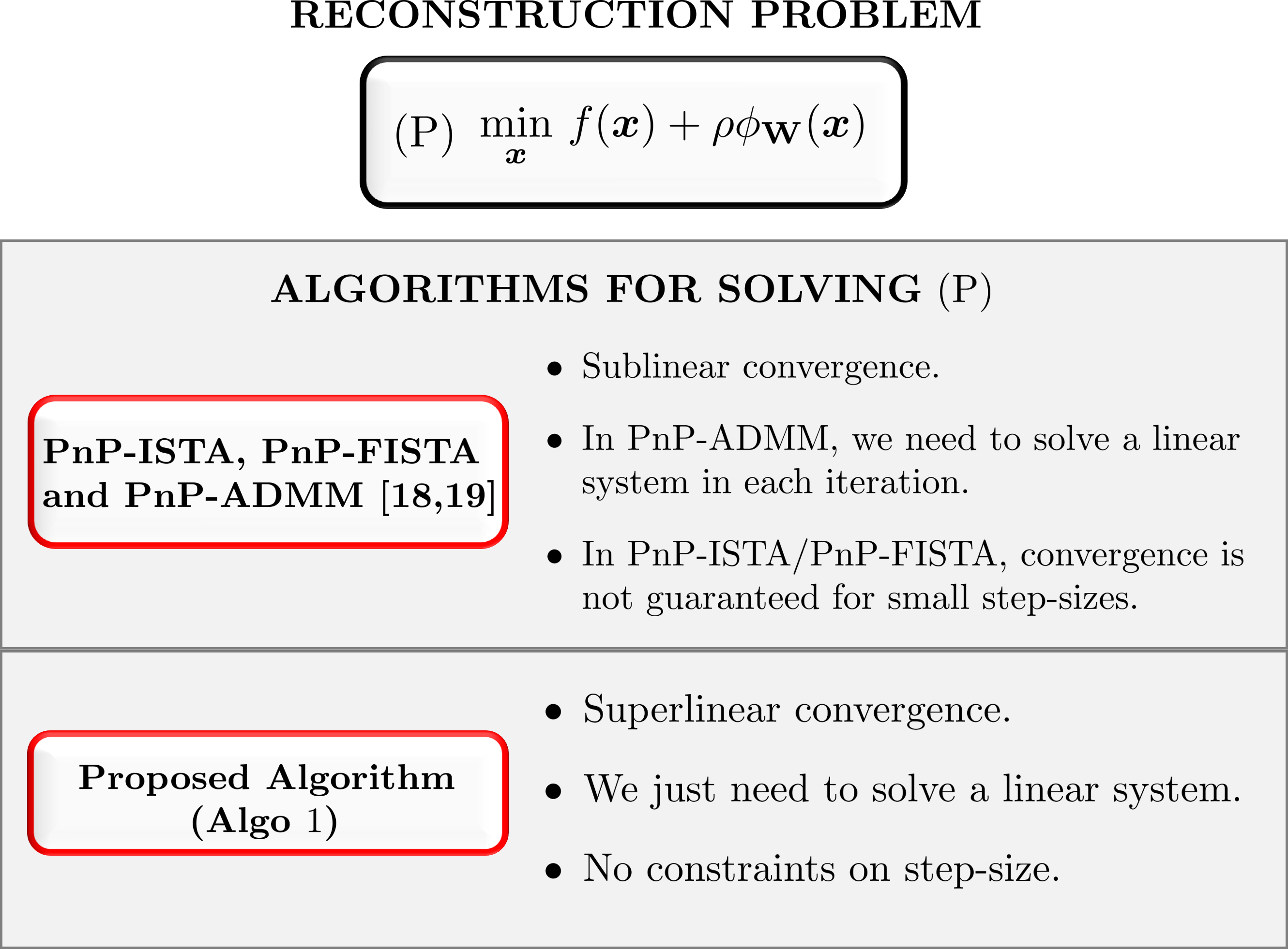
Figure 2: Relation of the proposed algorithm with the PnP algorithms in [19, 18] for a linear denoiser $\mathbf{W}$. The reconstruction returned by such algorithms is a minimizer of a convex objective function $f+\Phi_{\mathbf{W}}$. Instead of iteratively computing the minimizer (as done in PnP algorithms), we propose to solve the first-order optimality condition for the problem, which can be reduced to solving a linear system if $f$ is quadratic. See Table I for more details.

I-B Motivation and contribution

The present work is best motivated using an analogy with least-squares regression. Suppose that we want to minimize ${\lVert\mathbf{H}\boldsymbol{x}-\boldsymbol{b}\rVert}^{2}$ with respect to $\boldsymbol{x}$. Among other things, we can compute the minimizer using either an iterative algorithm such as the gradient descent method or via the solution of the normal equation $\mathbf{H}^{\top}\!\mathbf{H}=\mathbf{H}^{\top}\!\boldsymbol{b}$ [44]. Recall that the normal equation is the first-order optimality condition for the optimization problem at hand. In particular, if $\mathbf{H}$ has full column rank, then we can solve the normal equation using conjugate gradient, which has superior convergence than the sublinearly-convergent gradient descent [45]. Similarly, our main idea is that instead of the iterative minimization in (5) and (6), which in effect minimizes $f+\Phi$, we can directly work with the first-order optimality condition and come up with an efficient algorithm (see Fig. 2). The technical novelty in this regard are:

• We prove that the minimization of $f+\Phi$ is well-posed, i.e., $f+\Phi$ is guaranteed to have a minimizer $\boldsymbol{x}^{\ast}\in\mathbb{R}^{n}$ (Proposition 5). Moreover, we prove that $\boldsymbol{x}^{\ast}$ is unique for some imaging problems (Proposition 6).

• We show that $\boldsymbol{x}^{\ast}$ can be computed by solving $\mathbf{A}\boldsymbol{x}=\boldsymbol{b}$. In particular, we prove that $\mathbf{A}$ is nonsingular for some reconstruction problems.

• On the computational side, we show how $\boldsymbol{x}^{\ast}$ can be accurately computed in just few iterations using superlinearly convergent solvers such as GMRES [46], LGMRES [47], GCROT [48] and Broyden [49, 50], where each iteration requires us to apply $\mathbf{F}$, $\mathbf{F}^{\top}$ and a kernel denoiser. Stated differently, we can obtain the same reconstruction as PnP-ISTA and PnP-ADMM, but unlike PnP-ISTA and PnP-ADMM which are known to converge sublinearly [17, 51], we can achieve superlinear convergence (see Fig. 2 for a comparison of our and existing PnP solvers). The speedup is apparent in practice as well. Moreover, thanks to the superior convergence rate, the total inference time of our solvers (number of iterations $\times$ time per iteration) are comparable with PnP algorithms with CNN-based denoisers, though CNN-based denoisers are faster than kernel denoisers.

A sample inpainting result obtained using our algorithm is shown in Fig. 1, where the text is almost completely removed from the image. Surprisingly, for superresolution, deblurring, and inpainting, we are able to get close to state-of-the-art methods in terms of reconstruction quality. This demonstrates that as a natural image prior, $\Phi$ is more effective than classical wavelet and total-variation priors. Understanding this in greater depth is left to future work.

I-C Organization

The paper is organized as follows. We present some background material about kernel denoisers in Section II-A and existing results on the optimality of PnP algorithms for kernel denoisers in Section II-B. We then explain the proposed work in Section III in three different subsections. In Section III-A, we provide a different formulation of the regularizer associated with the PnP algorithms in [19, 18]. In Section III-B, we show how the task of minimizing $f+\Phi$ can be reduced to solving a linear system. In Section III-C, we present our algorithm and perform ablation studies on it; in particular, we experiment with different numerical solvers and demonstrate their effectiveness over existing PnP solvers. In Section IV, we present results for superresolution, deblurring, and inpainting, and compare our method with top-performing methods. We conclude with a discussion of our findings in Section V. Proofs of technical results are deferred to Section VI.

II Background

II-A Kernel denoiser

A kernel filter can abstractly be viewed as a linear transform $\mathbf{W}\in\mathbb{R}^{n\times n}$ that takes a noisy image $\boldsymbol{x}\in\mathbb{R}^{n}$ and returns the denoised output $\mathbf{W}\boldsymbol{x}$, where $\boldsymbol{x}$ is some vectorized form of the image and $n$ is the number of pixels. We now explain this more precisely which will require some notations.

Let us denote the input image as $\{X_{\boldsymbol{s}}:\boldsymbol{s}\in\Omega\}$, where $\Omega\subset\mathbb{Z}^{2}$ is the support of the image and $X_{\boldsymbol{s}}$ is the intensity value at pixel location $\boldsymbol{s}$. The essential point is that $\mathbf{W}$ is defined using a symmetric positive definite kernel $\phi:\mathcal{F}\times\mathcal{F}\to\mathbb{R}$, where the feature space $\mathcal{F}$ is stipulated using a guide image $\{\boldsymbol{u}_{\boldsymbol{s}}:\boldsymbol{s}\in\Omega\}$. This is usually the input image for image denoising [10]. However, in PnP regularization, the guide $\boldsymbol{u}$ is a surrogate of the ground-truth image $\boldsymbol{\theta}$ which is computed from the measurement [15, 19, 18]. The feature space in NLM is $\mathcal{F}=\mathbb{R}^{2+p}$, where $p$ is the size of a pre-fixed square patch $P$ centered at the origin. In particular, the feature vector $\boldsymbol{\zeta}_{\boldsymbol{s}}\in\mathcal{F}$ at pixel $\boldsymbol{s}\in\mathbb{Z}^{2}$ is obtained by concatenating the pixel position $\boldsymbol{s}$ and the intensity values $\{\boldsymbol{u}_{\boldsymbol{s}+\boldsymbol{\tau}}:\boldsymbol{\tau}\in P\}\in\mathbb{R}^{p}$ from a patch around $\boldsymbol{s}$ in the guide image. The kernel in NLM is typically Gaussian and is defined as $\phi(\boldsymbol{q},\boldsymbol{r})=G(\boldsymbol{q}-\boldsymbol{r})$, where $G$ is a multivariate Gaussian on $\mathcal{F}$ [52, 53]. The NLM operator $\mathfrak{D}$ which takes input $X$ and outputs image $\mathfrak{D}(X)$ is defined as

$$\forall\ \boldsymbol{s}\in\Omega:\quad{(\mathfrak{D}(X))}_{\boldsymbol{s}}=\frac{\sum_{\boldsymbol{t}\in\Omega}\phi({\boldsymbol{\zeta}}_{\boldsymbol{s}},{\boldsymbol{\zeta}}_{\boldsymbol{t}})X_{\boldsymbol{t}}}{\sum_{\boldsymbol{t}\in\Omega}\phi({\boldsymbol{\zeta}}_{\boldsymbol{s}},{\boldsymbol{\zeta}}_{\boldsymbol{t}})}.$$ (7)

In other words, the output at a given pixel is obtained using a weighted average of its neighboring pixels, where the weights are derived from the similarity between features $\boldsymbol{\zeta}_{\boldsymbol{s}}$ and $\boldsymbol{\zeta}_{\boldsymbol{t}}$ measured using kernel $\phi$.

It is clear from (7) that $\mathfrak{D}$ is a linear operator. To obtain the matrix representation of (7), we need to linearly index the pixel space $\Omega$. Let $\sigma:[1,n]\to\Omega$ be such that every index $\ell\in[1,n]$ is mapped to a unique pixel $\sigma(\ell)\in\Omega$. Let $\boldsymbol{x}$ be the vector representation of $X$ corresponding to this indexing, so that $\boldsymbol{x}_{\ell}=X_{\sigma(\ell)}$ for $\ell\in[1,n]$. Now, define the kernel matrix $\mathbf{K}\in\mathbb{R}^{n\times n}$ to be

$$\forall i,j\in[1,n]:\quad\mathbf{K}_{ij}=\phi(\boldsymbol{\zeta}_{\sigma(i)},\boldsymbol{\zeta}_{\sigma(j)}),$$

and the diagonal matrix $\mathbf{D}\in\mathbb{R}^{n\times n}$ to be $\mathbf{D}_{ii}=\sum_{j=1}^{n}\mathbf{K}_{ij}$ for $i\in[1,n]$. We can then express (7) as the linear transform $\boldsymbol{x}\to\mathbf{W}\boldsymbol{x}$, where

$$\mathbf{W}:=\mathbf{D}^{-1}\mathbf{K}.$$ (8)

By construction, both $\mathbf{K}$ and $\mathbf{D}$ are symmetric; $\mathbf{K}$ is positive semidefinite and $\mathbf{D}$ is positive definite [54]. We note that apart from image denoising [10, 41, 55, 56, 57], kernel filters have also been used for graph signal processing [26, 28, 27].

II-B Kernel denoiser as a proximal operator

Kernel filters, and in particular NLM-type denoisers, have been shown to be very effective for PnP regularization [15, 55, 56, 57]. In this section, we discuss existing results on the optimality of the PnP reconstruction obtained using a kernel denoiser.

Recall that in PnP, we replace the proximal operator $\mathrm{prox}_{g}$ in (4) by a denoiser $\mathfrak{D}$ in (5). The question is whether we can express a given denoiser as a proximal operator of some convex regularizer—convergence of the PnP iterates and optimality of the final reconstruction would immediately be settled if we can answer this in the affirmative. This question remains open for complex denoisers such as BM3D and DnCNN. However, it has been shown in [19, 18] that for the kernel filter given by (8), one can indeed construct a convex regularizer $g$ such that $\mathbf{W}=\mathrm{prox}_{g}$. We need some notations and definitions to explain this technical result.

Since $\mathbf{D}$ is positive definite, we can define the following inner product and norm on $\mathbb{R}^{n}$:

$${\left\langle\boldsymbol{x},\boldsymbol{y}\right\rangle}_{\mathbf{D}}=\boldsymbol{x}^{\top}\!\mathbf{D}\boldsymbol{y}\quad\text{and }\quad\left\lVert\boldsymbol{x}\right\rVert_{\mathbf{D}}=\left\langle\boldsymbol{x},\boldsymbol{x}\right\rangle^{1/2}_{\mathbf{D}}.$$ (9)

The latter can be viewed as a weighted $\ell_{2}$ norm. We associate a proximal operator with this norm.

Definition 1.

Let $g:\mathbb{R}^{n}\to\mathbb{R}\cup\{\infty\}$ be closed, proper and convex. Define $\mathrm{prox}_{g,\mathbf{D}}:\mathbb{R}^{n}\to\mathbb{R}^{n}$ to be

$$\mathrm{prox}_{g,\mathbf{D}}(\boldsymbol{x})=\mathop{\mathrm{argmin}}_{\boldsymbol{z}\in\mathbb{R}^{n}}\ \left\{\frac{1}{2}\left\lVert\boldsymbol{z}-\boldsymbol{x}\right\rVert_{\mathbf{D}}^{2}+g(\boldsymbol{z})\right\},$$ (10)

We call $\mathrm{prox}_{g,\mathbf{D}}$ the scaled proximal operator of $g$.

The term “scaled” is used to emphasize that the weighted $\ell_{2}$ norm is used in (10). It is well-known that the objective in (10) has a unique minimizer for the standard $\ell_{2}$ norm and that $\mathrm{prox}_{g}$ is well-defined [58]; it is not difficult to verify that this is also true for the weighted norm.

The authors in [19, 18] showed that a kernel denoiser is a scaled proximal operator of a convex regularizer. This observation was used to establish objective and iterate convergence. We recall the exact formula for this regularizer which will play a central role in the rest of the discussion.

It can be shown that the kernel filter is diagonalizable. In particular, let $\mathbf{W}=\mathbf{V}\boldsymbol{\Lambda}\mathbf{V}^{-1}$ be the eigendecomposition of (8), where the columns of $\mathbf{V}$ are the eigenvectors of $\mathbf{W}$ and $\boldsymbol{\Lambda}$ is a diagonal matrix whose first $r$ diagonal entries are in $(0,1]$ and the remaining entries are $0$. We collect the $r$ positive eigenvalues in a diagonal matrix $\boldsymbol{\Lambda}_{r}$ and the corresponding eigenvectors in $\mathbf{U}\in\mathbb{R}^{n\times r}$. Then we can write $\mathbf{W}=\mathbf{U}\boldsymbol{\Lambda}_{r}\mathbf{U}^{\dagger}$, where $\mathbf{U}^{\dagger}\in\mathbb{R}^{r\times n}$ consists of the first $r$ rows of $\mathbf{V}^{-1}$. The authors in [18] showed that $\mathbf{W}$ is a scaled proximal operator of the extended-valued convex function

$$\Phi_{\mathbf{W}}(\boldsymbol{x})=\begin{cases}\dfrac{1}{2}\boldsymbol{x}^{\top}{\mathbf{U}^{\dagger}}^{\top}(\boldsymbol{\Lambda}_{r}^{-1}-\mathbf{I})\mathbf{U}^{\dagger}\boldsymbol{x},&\mathrm{for}\ \boldsymbol{x}\in\mathcal{R}(\mathbf{W}).\\[5.0pt] \infty,&\mathrm{otherwise},\end{cases}$$ (11)

Note that $\Phi_{\mathbf{W}}$ is completely determined by the kernel denoiser $\mathbf{W}$. Its domain is restricted to $\mathcal{R}(\mathbf{W})$ and this in effect forces the reconstruction to be in $\mathcal{R}(\mathbf{W})$.

III Kernel Regularization

III-A PnP regularization using kernel denoiser

We first propose an alternate formulation for the regularizer in (11) and prove that the scaled proximal operator of (11) is indeed $\mathbf{W}$. Apart from keeping the account self-contained, our formulation makes the proofs simpler and helps in analyzing the optimization problem in (2) with $g=\Phi_{\mathbf{W}}$.

Note that $\mathbf{W}$ is not symmetric, but it can be written as

$$\mathbf{W}=\mathbf{D}^{-1/2}\mathbf{S}\mathbf{D}^{1/2},\quad\mathbf{S}:=\mathbf{D}^{-1/2}\mathbf{K}\mathbf{D}^{-1/2}.$$

Thus, $\mathbf{W}$ is similar to the symmetric matrix $\mathbf{S}$ and is hence diagonalizable with real eigenvalues. More specifically, if $\mathbf{S}=\mathbf{Q}\boldsymbol{\Lambda}\mathbf{Q}^{\top}\!$ is an eigendecomposition of $\mathbf{S}$, then we can write

$$\mathbf{W}=\mathbf{M}\boldsymbol{\Lambda}\mathbf{M}^{-1},\quad\mathbf{M}:=\mathbf{D}^{-1/2}\mathbf{Q}.$$

Define $\mathbf{W}^{\dagger}=\mathbf{M}\boldsymbol{\Lambda}^{\dagger}\mathbf{M}^{-1}$, where $\boldsymbol{\Lambda}^{\dagger}$ is diagonal and $\boldsymbol{\Lambda}^{\dagger}_{ii}=\boldsymbol{\Lambda}_{ii}^{-1}$ if $\boldsymbol{\Lambda}_{ii}>0$, and $\boldsymbol{\Lambda}^{\dagger}_{ii}=0$ otherwise. We remark that $\mathbf{W}^{\dagger}$ is the generalized inverse of $\mathbf{W}$ and that $\mathbf{W}=\mathbf{W}\mathbf{W}^{\dagger}\mathbf{W}$ [59].

Definition 2.

Let $\mathbf{W}$ be a kernel denoiser. Define the function $\Phi_{\mathbf{W}}:\mathbb{R}^{n}\to\mathbb{R}\cup\{\infty\}$ to be

$$\Phi_{\mathbf{W}}(\boldsymbol{x})=\begin{cases}\dfrac{1}{2}\boldsymbol{x}^{\top}\mathbf{D}(\mathbf{I}-\mathbf{W})\mathbf{W}^{\dagger}\boldsymbol{x},&\mathrm{for}\ \boldsymbol{x}\in\mathcal{R}(\mathbf{W}),\\[5.0pt] \infty,&\mathrm{otherwise}.\end{cases}$$ (12)

We call $\Phi_{\mathbf{W}}$ the kernel regularizer associated with $\mathbf{W}$.

The extended-valued function $\Phi_{\mathbf{W}}$ is quadratic on its domain. Moreover, we have the following properties.

Proposition 3.

$\Phi_{\mathbf{W}}$ is nonnegative, closed (epigraph is closed in $\mathbb{R}^{n+1}$), proper (domain is nonempty), and convex.

In particular, it follows from Proposition 3 that $\mathrm{prox}_{\Phi_{\mathbf{W}},\mathbf{D}}$ is well-defined. This brings us to the key result—the characterization of a kernel denoiser as a proximal operator.

Theorem 4.

$\mathbf{W}$ is a scaled proximal operator of $\Phi_{\mathbf{W}}$, i.e.,

$$\forall\ \boldsymbol{x}\in\mathbb{R}^{n}:\quad\mathbf{W}\boldsymbol{x}=\mathrm{prox}_{\Phi_{\mathbf{W}},\mathbf{D}}(\boldsymbol{x}).$$

We now relate the above results to the PnP updates in (5) and (6) where the denoiser is $\mathfrak{D}=\mathbf{W}$. In this case, it follows from Theorem 4 that we can write (5) as

$$\boldsymbol{x}_{k+1}=\mathrm{prox}_{\Phi_{\mathbf{W}},\mathbf{D}}\big{(}\boldsymbol{x}_{k}-\rho^{-1}\nabla\!f(\boldsymbol{x}_{k})\big{)}.$$ (13)

This looks like standard ISTA [17, 58], except that we have the scaled proximal operator instead of the standard proximal operator. In particular, if we replace $\nabla\!f$ (gradient of $f$ w.r.t. $\ell_{2}$ norm) in (13) with $\mathbf{D}^{-1}\nabla\!f$ (gradient of $f$ w.r.t. weighted-$\ell_{2}$ norm), then PnP updates amount to minimizing $f+\rho\Phi_{\mathbf{W}}$ [19, 18]. Similarly, we can write the PnP-ADMM updates as

$$\boldsymbol{x}_{k+1}=\underset{\boldsymbol{x}}{\mathrm{argmin}}\ f(\boldsymbol{x})+\frac{1}{2\rho}\|\boldsymbol{x}-(\boldsymbol{v}_{k}-\boldsymbol{z}_{k})\|_{\mathbf{D}}^{2},$$ (14)

$$\boldsymbol{v}_{k+1}=\mathrm{prox}_{\Phi_{\mathbf{W}},\mathbf{D}}(\boldsymbol{x}_{k+1}+\boldsymbol{z}_{k}),$$

$$\boldsymbol{z}_{k+1}=\boldsymbol{z}_{k}+(\boldsymbol{x}_{k+1}-\boldsymbol{v}_{k+1}),$$

Again, this looks like standard ADMM except that the weighted $\ell_{2}$ norm is used instead of the standard $\ell_{2}$ norm for the $\boldsymbol{x}$ update. In summary, if we use a kernel denoiser for PnP regularization and we make some minor algorithmic adjustments to the PnP updates, the resulting iterates are guaranteed to converge to the minimum of $f+\rho\Phi_{\mathbf{W}}$. Thus, the seemingly ad-hoc idea of “plugging” a denoiser into the reconstruction process does amount to solving a regularization problem if we use a kernel denoiser.

Having been able to associate an optimization problem with the PnP iterations, a natural question is whether we can solve the optimization problem more efficiently. This would provide an alternate means for performing PnP regularization. We next show that this is indeed the case for linear inverse problems.

III-B Reduction to a linear system

Recall from the previous discussion that PnP regularization using a kernel denoiser amounts to solving (2), where $f$ and $g$ are given by (3). In other words, the optimization problem associated with PnP-ISTA and PnP-ADMM is

$$\underset{\boldsymbol{x}\in\mathcal{R}(\mathbf{W})}{\mathrm{min}}\ \left\{\frac{1}{2}\|\boldsymbol{y}-\mathbf{F}\boldsymbol{x}\|^{2}_{2}+\frac{\rho}{2}\boldsymbol{x}^{\top}\mathbf{D}(\mathbf{I}-\mathbf{W})\mathbf{W}^{\dagger}\boldsymbol{x}\right\}.$$ (15)

It is not obvious if (15) has a minimizer since $\mathbf{F}$ has a non-trivial null space [60]. In [19, 18], the authors have assumed the existence of a minimizer without proof. We now establish this rigorously.

Proposition 5.

The optimization problem (15) is solvable. In particular, consider the linear system $\mathbf{A}\boldsymbol{z}=\boldsymbol{b}$, where

$$\mathbf{A}=\mathbf{W}^{\top}\mathbf{F}^{\top}\mathbf{F}\mathbf{W}+\rho\mathbf{W}^{\top}\mathbf{D}(\mathbf{I}-\mathbf{W}),\ \ \boldsymbol{b}=\mathbf{W}^{\top}\mathbf{F}^{\top}\boldsymbol{y}.$$ (16)

Then $\mathbf{A}\boldsymbol{z}=\boldsymbol{b}$ is solvable. Moreover, $\boldsymbol{x}^{\ast}$ is a minimizer of (15) if and only if $\boldsymbol{x}^{\ast}=\mathbf{W}\boldsymbol{z}$ where $\boldsymbol{z}$ is a solution of $\mathbf{A}\boldsymbol{z}=\boldsymbol{b}$.

We remark that although $\mathbf{W}^{\dagger}$ appears in (15), it does not come up in (16). This is important since computing $\mathbf{W}^{\dagger}$ from $\mathbf{W}$ via its eigendecomposition would be impractical given the black-box nature of $\mathbf{W}$ and its size. On the other hand, note that $\mathbf{W}^{\top}=\mathbf{D}\mathbf{W}\mathbf{D}^{-1}$. Hence, computing $\mathbf{W}^{\top}\boldsymbol{x}$ has the same cost as that of computing $\mathbf{W}\boldsymbol{x}$ since $\mathbf{D}$ is a diagonal matrix.

Though the linear system $\mathbf{A}\boldsymbol{z}=\boldsymbol{b}$ is solvable, $\mathbf{A}$ can nevertheless be singular. However, most iterative linear solvers in their original form (e.g. Krylov methods) require $\mathbf{A}$ to be nonsingular for theoretical convergence [61]. The following proposition is useful in this regard.

Proposition 6.

Let $\boldsymbol{e}\in\mathbb{R}^{n}$ be the all-ones vector. If $\mathbf{W}$ is nonsingular and $\mathbf{F}\boldsymbol{e}\neq\mathbf{0}$, then $\mathbf{A}$ is nonsingular.

For deblurring, superresolution and inpainting, $\mathbf{F}$ trivially satisfies the hypothesis in Proposition 6 since $\boldsymbol{e}$ does not belong to the null space of $\mathbf{F}$. On the other hand, for bilateral and NLM filters, $\mathbf{W}$ is nonsingular if the spatial component of the kernel function $\phi$ is a hat function [19, Theorem $3.13$].

Note that if $\mathbf{W}$ is nonsingular, then $\mathbf{A}\boldsymbol{z}=\boldsymbol{b}$ can equivalent be expressed as $\mathbf{C}\boldsymbol{z}=\boldsymbol{d}$, where

$$\mathbf{C}=\mathbf{F}^{\top}\mathbf{F}\mathbf{W}+\rho\mathbf{D}(\mathbf{I}-\mathbf{W})\quad\text{and}\quad\boldsymbol{d}=\mathbf{F}^{\top}\boldsymbol{y}.$$ (17)

The advantage with (17) compared to (16) is that $\mathbf{W}^{\top}$ does not appear in $\mathbf{C}$. However, unlike $\mathbf{A}$, $\mathbf{C}$ is no longer guaranteed to be symmetric.

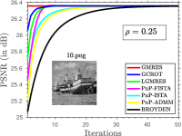
(a)

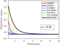
(b)

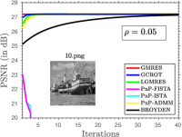
(c)

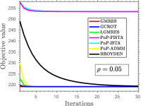
(d)

Figure 3: Comparison of the efficiency of iterative solvers for image deblurring. A Gaussian blur of $25\times 25$ and standard deviation $1.6$ is used and the noise level is $\sigma=10/255$. The plots show the evolution of PSNR and objective function (15) for $\rho=0.25$ (left column) and $\rho=0.05$ (right column). We have used NLM as the denoiser. The comparison is between PnP-ISTA, PnP-FISTA and PnP-ADMM [19, 18] and the proposed linear solvers GMRES, GCROT and LGMRES. As expected, our solvers exhibit faster convergence than the iterative minimization of (15) using PnP-ISTA, PnP-FISTA and PnP-ADMM. For example, GCROT requires just $40\%$ percent of the iterations taken by PnP-ADMM to stabilize. Note that PnP-ISTA and PnP-FISTA diverges when $\rho=0.05$.

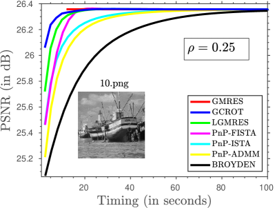
(a)

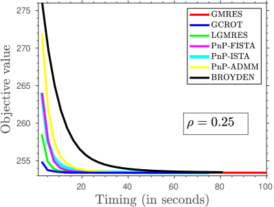
(b)

Figure 4: Efficiency comparison of the algorithms for the experiment in Fig. 3. The linear solvers are faster to stabilize than the iterative minimization of (15) using PnP algorithms.

III-C Proposed algorithm

Input: Measurements $\boldsymbol{y}$ and forward operator $\mathbf{F}$.

Output: Solution of (15).

1 Form the guide image $\boldsymbol{u}$ from measurements $\boldsymbol{y}$;

2 Construct the denoising operator $\mathbf{W}$ from $\boldsymbol{u}$;

3 Use $\mathbf{W}$ and $\mathbf{F}$ to construct operator $\mathbf{C}$;

4 Solve $\mathbf{C}\boldsymbol{z}=\mathbf{F}^{\top}\boldsymbol{y}$ ;

Return $\mathbf{W}\boldsymbol{z}$.

Algorithm 1 Regularization using a linear solver

The overall algorithm stemming from the previous discussion is summarized in Algorithm 1. In the first step, the guide image $\boldsymbol{u}$ is derived from the measurements $\boldsymbol{y}$ using about $5\mbox{-}10$ PnP iterations, as done in [15, 62, 19, 18]. This is used to construct the kernel denoiser $\mathbf{W}$ and in turn the operator $\mathbf{C}$. We choose NLM as the preferred kernel denoiser because of its superior regularization capabilities, where the features are derived from the guide image $\boldsymbol{u}$ as explained in Section II-A. The final and core step is the solution of $\mathbf{C}\boldsymbol{z}=\mathbf{F}^{\top}\boldsymbol{y}$. We have used iterative solvers such as LGMRES and GCROT (using linalg module in the scipy package). which seem to provide the best tradeoff between iteration complexity and the number of iterations required to converge. This is highlighted in Fig. 3.

At this point, we wish to clarify that $\mathbf{W}$, $\mathbf{F}$ and $\mathbf{F}^{\top}$ in (17) are not stored as matrices. Rather, they are implemented efficiently as input-output black boxes. Indeed, $\mathbf{W}\boldsymbol{x}$ can be computed directly from (7). For deblurring, $\mathbf{F}$ and $\mathbf{F}^{\top}$ are implemented using spatial convolution (narrow blur) or FFT (wide blur). For superresolution, $\mathbf{F}$ is implemented using spatial convolution followed by decimation and $\mathbf{F}^{\top}$ is implemented using upsampling followed by convolution. For inpainting, computing $\mathbf{F}$ (and $\mathbf{F}^{\top}=\mathbf{F}$) amounts to sampling the observed pixels.

(a)

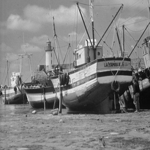
(b)

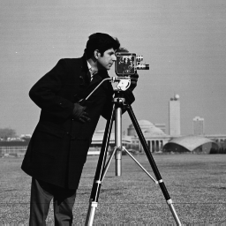
(c)

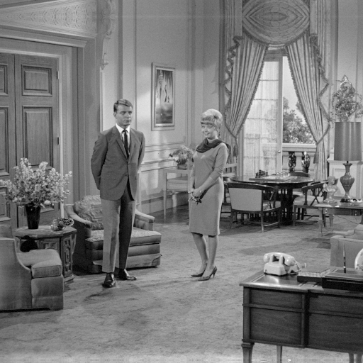
(d)

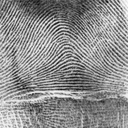
(e)

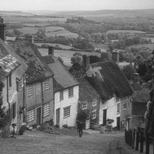
(f)

(g)

(h)

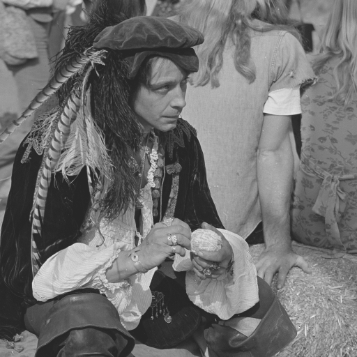
(i)

Figure 5: Grayscale input images used in the experiments in this paper.

TABLE I: Comparison of the PnP algorithms in [19, 18] and the proposed solver.

Property	PnP algorithms [19, 18]	Proposed	Comments
convergence rate	sublinear convergence	superlinear convergence	superior convergence rate of our method is empirically seen in Fig. 3.
cost per iteration	more for PnP-ADMM in most applications since we need to solve a linear system	same as PnP-ISTA	total time taken to stabilize is less for our method as shown in Fig. 4.
flexibility of step size $\rho$	$\rho\geqslant 0.5\sigma_{\mathrm{max}}(\mathbf{D}^{-1/2}\mathbf{F}^{\top}\mathbf{F}\mathbf{D}^{-1/2})$ to guarantee convergence for PnP-ISTA	convergent for any $\rho>0$	as seen in Fig. 3, $\rho$ needs to be small to obtain state-of-the-art results.
existence of minimizer of (15)	assumed	proved in Proposition 5	we can certify this for general linear inverse problems.
unique minimizer of (15)	not discussed	proved in Proposition 6	uniqueness can be certified for deblurring, inpainting and superresolution.

TABLE II: Comparison of PSNR using different number of PnP iterations to obtain the guide image from the measurements.

	Deblurring						Inpainting
# PnP iterations	$0$	$1$	$2$	$3$	$4$	$5$	$0$	$1$	$2$	$3$	$4$	$5$
barbara	23.88	$23.81$	$23.88$	$23.82$	$23.81$	$23.79$	$24.16$	$23.10$	$23.58$	$24.81$	$26.11$	27.19
boat	$27.22$	$27.36$	27.46	$27.30$	$27.22$	$27.11$	$26.93$	$27.47$	$27.57$	$27.70$	$27.87$	27.99
cameraman	$24.59$	$24.67$	24.78	$24.68$	$24.62$	$24.54$	$23.55$	$24.29$	$24.48$	$24.64$	$24.80$	24.93
couple	$26.74$	$26.92$	27.00	$26.95$	$26.89$	$26.82$	$26.81$	$27.09$	$27.21$	$27.45$	$27.72$	27.90
fingerprint	25.88	$25.78$	$25.27$	$24.73$	$24.36$	$24.00$	$23.52$	$25.14$	$25.36$	$25.63$	$25.94$	26.20
hill	$28.16$	$28.15$	28.27	$28.15$	$28.15$	$28.13$	$28.86$	$28.90$	$28.96$	$29.06$	$29.18$	29.27
house	29.96	$29.48$	$29.62$	$29.37$	$29.92$	$29.14$	$29.34$	$30.48$	$30.86$	$31.32$	$31.82$	32.17
lena	$30.32$	$30.24$	30.43	$30.25$	$30.19$	$30.08$	$30.35$	$31.05$	$31.23$	$31.46$	$31.67$	31.84
man	$28.06$	$28.06$	28.17	$28.05$	$28.00$	$27.91$	$28.16$	$28.39$	$28.48$	$28.62$	$28.77$	28.87

III-D Comparison with existing PnP algorithms

We remark that the optimization in (15) can be solved using either existing PnP algorithms [19, 18] or the proposed linear solver (17). Moreover, both are iterative in nature. An obvious question is what advantage does the latter offer? In this regard, we wish to discuss the following points.

• For solving linear systems, Krylov solvers like GMRES, GCROT and LGMRES are known to be superlinearly convergent [61]. On the other hand, iterative PnP algorithms such as PnP-ISTA, PnP-FISTA and PnP-ADMM are only sublinearly convergent [17, 51]. Hence, in theory, Algorithm 1 with Krylov solvers should require fewer iterations as compared to the PnP algorithms in [19, 18]. We have experimented using Krylov solvers GMRES [46], LGMRES [47], GCROT [48] and the quasi-Newton Broyden solver [49, 50]. The evolution of the objective function and PSNR for a deblurring experiment is shown in Fig. 3 for $\rho\in\{0.05,0.25\}$. Compared to PnP-ISTA, PnP-FISTA and PnP-ADMM algorithms [19, 18], Algorithm (1) indeed converges much faster to a minimizer of $f+\rho\Phi_{\mathbf{W}}$, regardless of the linear solver used. Based on the convergence rate, we can order them as follows: GMRES ($12$s) $>$ GCROT ($2.5$s) $>$ LGMRES ($2.5$s) $>$ PnP-ISTA, PnP-FISTA, PnP-ADMM ($2.5$s) $>$ Broyden ($2.7$s), where the per-iteration cost is mentioned within brackets. We note that the per-iteration cost of GCROT and LGMRES is comparable to that of the PnP algorithms in [19, 18] but they converge much faster.

• For our proposal, we are required to solve just one linear system. On the contrary, in every iteration of PnP-ADMM (14), the following linear system needs to be solved as part of the $\boldsymbol{x}$ update (outer iterations):

  $$(\mathbf{F}^{\top}\mathbf{F}+\mathbf{D})\boldsymbol{x}_{k+1}=\mathbf{F}^{\top}\boldsymbol{y}+\mathbf{D}(\boldsymbol{v}_{k}-\boldsymbol{z}_{k}).$$

  This in turn requires an iterative solver (inner iterations) for deblurring and superresolution.

• In Fig. 3, notice that PnP-ISTA and PnP-FISTA diverges when $\rho$ is $0.05$. This is possibly because this choice of $\rho$ violates the bound $\rho\geqslant 0.5\ \sigma_{\mathrm{max}}(\mathbf{D}^{-1/2}\mathbf{F}^{\top}\mathbf{F}\mathbf{D}^{-1/2})$ that is used to guarantee convergence [19, 18]. On the other hand, our linear solver converges for any $\rho>0$. This is important since we often obtain better reconstructions for smaller $\rho$, e.g., PSNR of $27.2$ dB at $\rho=0.05$ compared to $26.35$ dB at $\rho=0.25$.

In summary, Algorithm 1 has several computational advantages over the PnP algorithms in [19, 18], though they solve the same optimization problem. A detailed comparison is provided in Table I.

III-E Comparison of convergent linear solvers

We consider four Krylov techniques for solving (17): GMRES, LGMRES, GCROT, and quasi-Newton Broyden. They come with convergence guarantees and can handle asymmetric systems. We have already shown in Section III-D that Algorithm 1 has a better convergence rate than PnP algorithms. Further, the evolution of the objective function (and PSNR) for a deblurring experiment is shown in Figures 3 and 4. Based on convergence rate (number of iterations), we can order them as follows: GMRES $>$ GCROT $>$ LGMRES $>$ Broyden, whereas based on the time taken to stabilize, the ordering is: GCROT $>$ LGMRES $>$ GMRES $>$ Broyden. We note that all four solvers solve the same optimization problem and hence stabilize to the same PSNR (objective) value. It is clear from the empirical analysis that GCROT offers an optimal tradeoff between convergence rate and cost per iteration.

(a) Ground truth

(b) Observed

(c) EPLL [8]

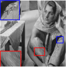
(d) IDBP-CNN [63]

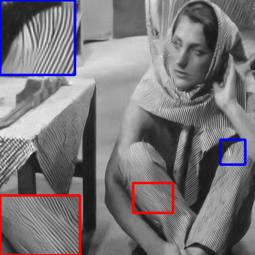
(e) PnP-CNN [21]

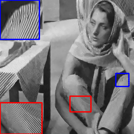
(f) Proposed.

Figure 6: Image inpainting from just $20\%$ pixels at $\sigma=10/255$ noise level. The proposed method ($\rho=0.05$) is compared with state-of-the-art methods (c)–(e). PSNR and SSIM values: (c) $24.87$ dB, $0.729$; (d) $26.12$ dB, $0.806$; (e) $26.99$ dB, $0.812$; and (f) 27.67 dB, 0.840. Comparison of the zoomed regions shows the superior reconstruction capability of our method in textured regions.

TABLE III: Experiment 1: Comparison of timing, PSNR and SSIM for Inpainting with $80$ percent missing pixels (Noiseless case).

Method	time (s)	barbara	boat	cameraman	couple	fingerprint	hill	house	lena	man
EPLL [8]	$258.13$	$25.43$ $0.792$	$27.51$ $0.788$	$24.31$ $0.816$	$27.69$ $0.801$	$24.20$ $0.845$	$29.06$ $0.776$	$30.71$ $0.867$	$30,42$ $0.867$	$27.94$ $0.795$
IRCNN[20]	$31.06$	$27.34$ $0.858$	$27.88$ $0.809$	$25.27$ $0.838$	$28.23$ $0.834$	$25.97$ $0.887$	$29.24$ $0.804$	$32.21$ $0.888$	$31.56$ $0.889$	$28.60$ 0.830
IDBP-BM3D [63]	$45.5$	$25.55$ $0.841$	$28.51$ 0.824	$24.86$ $0.840$	28.80 $0.846$	$25.09$ $0.878$	$29.74$ $0.810$	33.78 0.893	$32.13$ $0.893$	$28.65$ $0.824$
IDBP-CNN [63]	$39.77$	$24.29$ $0.796$	$27.72$ $0.803$	$24.24$ $0.826$	$27.98$ $0.818$	$25.59$ $0.865$	$29.01$ $0.790$	$32.14$ $0.881$	$31.22$ $0.880$	$28.58$ 0.830
Proposed - Yaroslavsky [38]	26.75	$29.14$ $0.884$	$27.88$ $0.767$	$25.10$ $0.816$	$28.07$ $0.792$	$26.68$ $0.913$	$28.96$ $0.758$	$32.12$ $0.850$	$31.25$ $0.853$	$28.32$ $0.719$
Proposed - Bilateral [40]	26.75	$29.37$ $0.896$	$28.24$ $0.817$	$24.85$ $0.842$	$28.56$ $0.840$	$26.34$ $0.902$	$29.53$ $0.823$	$32.83$ $0.829$	$31.98$ $0.894$	$28.80$ $0.819$
Proposed - NLM (Laplacian)	28.15	$29.32$ $0.890$	$28.28$ $0.821$	$25.07$ $0.828$	$28.64$ $0.845$	$26.29$ $0.900$	$29.75$ $0.823$	$33.43$ $0.895$	$32.06$ $0.894$	$28.82$ $0.829$
Proposed - NLM (Gaussian)	28.15	29.52 0.900	28.56 0.824	25.71 0.848	$28.72$ 0.849	26.45 0.908	29.78 0.825	$33.08$ $0.891$	32.42 0.896	28.90 $0.829$

III-F Choice of guide image

In Section III-C, the guide image $\boldsymbol{u}$ is derived from the measurements $\boldsymbol{y}$ using $5$ to $10$ PnP iterations, as done in [15, 62, 19, 18]. Note that the final reconstruction depends on the regularizer $\phi_{\mathbf{W}}$ in (12) and hence $\mathbf{W}$, and $\mathbf{W}$ in turn depends on the choice of guide. Intuitively, we should expect better reconstructions if the guide image resembles the ground truth, i.e., if we use more PnP iterations to compute the guide from the measurements—this is indeed the case with the inpainting results in Table II. However, this is not true in general. We empirically found that the dependence of the number of PnP iterations (used to compute the guide) on the reconstruction is complicated and depends on the image and application at hand. For example, from the deblurring results in Table II, we see that one or two iterations seem to give the best results. On the other hand, for the inpainting results in Table II, the reconstruction is seen to improve with the number of PnP iterations. We wish to investigate this aspect more thoroughly in future work.

IV Experimental Results

To understand the reconstruction capability of the proposed algorithm in relation to state-of-the-art methods, we apply our algorithm to three different inverse problems—inpainting, superresolution, and deblurring. In step (1) of Algorithm 1, we use the GCROT solver; we use just $5$ iterations which takes about $10$ seconds for a $512\times 512$ image. All experiments were performed on a $2.3$ GHz, $36$ core machine (no GPUs are used). The input images in Fig. 5 are used for comparisons. Timings are reported to highlight the speedup obtained using our algorithm.

TABLE IV: Experiment 2: Comparison of timing, PSNR and SSIM for Inpainting with $80$ percent missing pixels (noise level $0.04$ ).

Method	time(s)	barbara	boat	cameraman	couple	fingerprint	hill	house	lena	man
EPLL [8]	$257.30$	$24.76$	$26.59$	$23.88$	$26.70$	$23.31$	$27.86$	$29.10$	$28.95$	$26.99$
		$0.720$	$0.720$	$0.727$	$0.733$	$0.812$	$0.710$	$0.773$	$0.777$	$0.724$
IRCNN [20]	$31.10$	$25.94$	$26.86$	24.75	$26.98$	$24.71$	$27.90$	$30.61$	$29.94$	$27.01$
		$0.781$	$0.741$	$0.794$	$0.757$	$0.834$	$0.726$	$0.845$	$0.833$	$0.725$
IDBP-BM3D [63]	$39.97$	$25.03$	$27.02$	$24.68$	27.22	$24.99$	$28.00$	31.62	$30.14$	$27.24$
		$0.755$	$0.731$	$0.786$	$0.759$	$0.836$	$0.708$	$0.850$	$0.835$	$0.727$
IDBP-CNN [63]	$63.10$	$26.12$	$26.95$	$23.94$	$27.04$	$24.50$	$27.93$	$31.16$	30.17	$27.21$
		$0.753$	0.756	$0.791$	$0.773$	$0.857$	0.734	0.851	0.849	0.735
Proposed	28.30	27.67	27.16	$24.64$	$27.08$	25.92	28.04	$30.70$	$30.10$	27.39
		0.791	$0.746$	0.795	0.761	0.886	$0.732$	$0.835$	$0.833$	$0.717$

(a) Ground truth

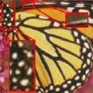
(b) Bicubic [64]

(c) TV [64]

(d) BM3D [11]

(e) DnCNN [21]

(f) Proposed

Figure 7: Results for $2\times$ image superresolution (using $9\times 9$ Gaussian blur with standard deviation $1$ and noise level $5/255$). Compared to BM3D (see zoomed regions), the quality is perceptibly better for PnP regularization, both for DnCNN and the proposed method ($\rho=2$). PSNR(dB), SSIM values: (b) $22.57$, $0.78$ (c) $24.3$, $0.83$ (d) $26.2$, $0.86$ (e) 27.4, $0.89$; and (f) $27.03$, 0.90.

TABLE V: Comparison of timing and PNSR for superresolution ($9\times 9$ Gaussian blur with standard deviation $1$, and noise level $5/255$).

Methods	time (s)	barbara	boat	cameraman	couple	fingerprint	hill	house	lena	man
$K=2$
SR[65]	$298.6$	$23.61$	$26.25$	$23.71$	$26.15$	$23.80$	$27.41$	$27.71$	$28.07$	$26.99$
GPR[66]	$390.12$	$23.82$	$26.81$	$23.91$	$26.63$	$24.05$	$28.38$	$29.16$	$29.54$	$27.78$
NCSR[9]	$256.16$	$24.67$	$28.40$	$26.22$	$28.02$	$27.74$	$28.50$	$29.85$	$30.43$	$28.75$
PnP-BM3D [16]	$48.65$	$24.64$	$29.41$	$26.73$	$29.22$	$28.82$	$29.82$	$32.65$	$32.76$	$29.66$
PnP-DnCNN [21]	$39.45$	$24.50$	29.57	27.36	$29.29$	$29.06$	$29.97$	$32.12$	$32.58$	29.98
Proposed	28.12	24.96	29.57	$26.74$	29.38	29.28	30.07	32.68	32.83	29.98
$K=4$
SR[65]	$298.6$	$20.67$	$21.30$	$18.86$	$21.51$	$16.37$	$23.15$	$22.19$	$22.85$	$22.26$
GPR[66]	$390.12$	$21.55$	$22.68$	$19.90$	$22.77$	$17.70$	$24.57$	$23.51$	$24.37$	$23.63$
NCSR[9]	$256.16$	$22.86$	$24.38$	$22.04$	$24.18$	$22.31$	$25.01$	$26.30$	$26.90$	$25.41$
PnP-BM3D [16]	$48.65$	$23.62$	25.75	$23.06$	25.30	$23.48$	$27.17$	29.14	$29.42$	$26.86$
PnP-DnCNN [21]	$39.45$	$23.66$	$25.73$	23.39	$25.27$	$23.61$	$27.19$	$29.05$	$29.44$	$26.92$
Proposed	28.12	23.67	$25.64$	$23.05$	25.30	23.65	27.20	$28.46$	29.45	26.93

TABLE VI: PSNR and SSIM on BSDS300 dataset for the inpainting experiments in Tables III and IV.

Methods	PnP-BM3D [16]	PnP-DnCNN [21]	Proposed
Experiment 1	$27.01$	$27.14$	27.15
	$0.8232$	0.8265	$0.8242$
Experiment 2	$25.59$	26.05	$26.00$
	$0.7485$	0.7584	$0.7493$

IV-A Inpainting

The problem in inpainting is to estimate missing pixels with known locations in an image; see [63] for the forward operator $\mathbf{F}$ in this case. A sample real-world application for removing text from an image was already shown in Fig. 1. Further, in Tables III and IV, we present an extensive comparison with state-of-the-art methods for image inpainting using just 20$\%$ pixels. Note that we are competitive with CNN-based methods [20] and [63], though we take less time. We note that solving the linear system in step $4$ of our algorithm takes about $10$ seconds and the remaining time is taken by step $1$ to construct the guide image. For the result in Fig. 6, we see that our method can preserve thin edges which the compared methods are unable to do. In Table VI, we shown that our algorithm is competitive with top performing methods on the BSDS300 dataset comprising of over $300$ images [67].

At this point, we wish to justify our choice of NLM as the preferred kernel denoiser. In Table III, we have compared the results using different kernel denoisers: bilateral, Yaroslavsky, standard NLM (Gaussian kernel) and NLM (Laplacian kernel). Since we consistently get the best results for standard NLM, we have used this denoiser for all experiments.

IV-B Superresolution

A widely used model for image superresolution is $\mathbf{F}=\mathbf{S}\mathbf{B}$, where $\mathbf{B}\in\mathbb{R}^{n\times n}$ is a blurring operator, $\mathbf{S}\in\mathbb{R}^{m\times n}$ is a subsampling operator, and $m=n/K$ where $K\geqslant 1$[16, 68]. In Table V, we compare with state-of-the art methods for $K=2$ and $4$, and using a Gaussian blur. Similar to inpainting, we are able to compete with state-of-the-art algorithms, while being faster. In Fig. 7, we compare our method with PnP-ADMM by plugging different denoisers. Notice that our method and PnP regularization using DnCNN [21] gives the best result. Unlike BM3D and TV, we are able to restore even fine features and do not over smooth the image.

IV-C Deblurring

The forward operator $\mathbf{F}$ is a blur in this case. We show a deblurring application in Fig. 8 where the blur kernel is asymmetric. Our method does not produce ringing artefacts as seen in a state-of-the-art method [20]. In Table VII, we perform three experiments as in [69] for different Gaussian blur and noise standard deviations. The results are averaged over the images in Fig. 5.

1. Gaussian blur $25\times 25$ and standard deviation $1.6$, and noise $\sigma=0.04$.

2. Gaussian blur $25\times 25$ and standard deviation $1.6$, and noise $\sigma=2/255$.

3. Gaussian blur $25\times 25$ and standard deviation $3$, and noise $\sigma=0.04$.

It is seen from Table VII that the proposed method is competitive with state-of-the-art deblurring methods [9, 20]. In Table VIII, we show that our method is generally competitive and can sometimes outperform the top methods [9, 20] on the BSDS300 dataset.

IV-D Discussion

It might seem surprising that NLM is able to compete with a pretrained deep denoiser for image regularization; after all, the denoising quality of DnCNN is generally a few dBs better than NLM. In this regard, we note that the exact relation between denoising capacity and the final restoration quality (within the PnP framework) is not well understood. For example, although DnCNN is more powerful than BM3D [12], it is known that plugging BM3D denoiser within a PnP algorithm can produce better results than DnCNN [21, 42]. Similarly, NLM has been shown to outperform BM3D (which is more powerful than NLM) for some applications [15, 70].

(a) Measurements

(b) IRCNN [20]

(c) Proposed

Figure 8: Image deblurring with an asymmetric blur kernel in [20]. Our result is visibly better than the learning-based method in [20].

TABLE VII: Comparison of PSNR for deblurring.

Method	Exp-I	Exp-II	Exp-III
EPLL [8]	$24.04$	$26.64$	$21.36$
MLP [69]	$24.76$	$27.23$	$22.20$
FlexISP [55]	$24.32$	$26.84$	$21.99$
LUT [7]]	$24.17$	$26.60$	$21.73$
[34]	$24.51$	$27.08$	$21.83$
DEB-BM3D [11]	$24.19$	$26.30$	$21.48$
NCSR [9]	$26.62$	$30.03$	$24.51$
IDD-BM3D [71]	$24.68$	$27.13$	$21.99$
IRCNN [20]	27.93	30.43	25.67
Proposed	27.70	30.40	25.62

TABLE VIII: PSNR and SSIM on the BSDS300 dataset for different deblurring experiments.

Methods	NCSR [9]	IRCNN [20]	Proposed
Exp 1	$25.56$	26.75	$26.25$
	$0.6707$	$0.7300$	0.7351
Exp 2	$28.97$	29.25	$28.57$
	$0.8338$	$0.8340$	0.8371
Exp 3	$24.01$	24.83	$24.33$
	$0.5527$	$0.6441$	0.6473

V Conclusion

This work builds on the observation that PnP regularization using kernel denoisers amounts to solving the classical regularization problem of minimizing $f+\Phi$, where $f$ is the loss term and $\Phi$ is a convex regularizer. We showed that for linear inverse problems with quadratic $f$, the first-order optimality condition for this problem can be reduced to a linear system, which is solvable and admits a unique solution for deblurring, superresolution, and inpainting. Instead of performing PnP iterations, we proposed to directly solve this linear system. Indeed, using efficient Krylov solvers, we could solve this linear system at a superlinear rate which is a big jump from the sublinear convergence guarantee of first-order PnP algorithms. We validated the speedup in practice using deblurring, superresolution, and inpainting experiments. In terms of reconstruction quality, we were able to get close to deep learning methods. A possible future work would be to apply our algorithm for hyperspectral imaging [72], where kernel filters can play a vital role for efficient high-dimensional denoising [73, 74].

VI Appendix

In this section, we state and prove the technical results in Section III. We first recall a few results from linear algebra and convex optimization.

VI-A Preliminaries

We will use $\mathcal{N}(\mathbf{Z})$ and $\mathcal{R}(\mathbf{Z})$ to denote the null space and range space of a matrix $\mathbf{Z}$.

Proposition 7.

Let $\mathbb{R}^{n}=U_{1}\oplus V_{1}=U_{2}\oplus V_{2}$, where $\oplus$ denotes orthogonal direct sum. Then $U_{1}\subseteq U_{2}$ implies $V_{2}\subseteq V_{1}$.

Proof.

Fix $\boldsymbol{x}\in V_{2}$. By our assumption, $\boldsymbol{x}\perp\boldsymbol{y}$ for all $\boldsymbol{y}\in U_{2}$. Since $U_{1}\subseteq U_{2}$, this mean that $\boldsymbol{x}$ belongs to the orthogonal complement of $U_{1}$, which is $V_{1}$ by assumption. ∎

Proposition 8.

Let $\mathbf{A},\mathbf{B}\in\mathbb{R}^{n\times n}$ be symmetric positive semidefinite matrices. Then $\mathcal{N}(\mathbf{A}+\mathbf{B})\subseteq\mathcal{N}(\mathbf{A})\cup\mathcal{N}(\mathbf{B})$ and $\mathcal{R}(\mathbf{A})\cup\mathcal{R}(\mathbf{B})\subseteq\mathcal{R}(\mathbf{A}+\mathbf{B})$.

Proof.

Let $\boldsymbol{x}\in\mathcal{N}(\mathbf{A}+\mathbf{B})$. Then $\boldsymbol{x}^{\top}(\mathbf{A}+\mathbf{B})\boldsymbol{x}=0$. However, by assumption, $\boldsymbol{x}^{\top}\mathbf{A}\boldsymbol{x}\geqslant 0$ and $\boldsymbol{x}^{\top}\mathbf{B}\boldsymbol{x}\geqslant 0$ for all $\boldsymbol{x}$. Thus $\boldsymbol{x}^{\top}(\mathbf{A}+\mathbf{B})\boldsymbol{x}=0$ only if $\boldsymbol{x}^{\top}\mathbf{A}\boldsymbol{x}=0$ and $\boldsymbol{x}^{\top}\mathbf{B}\boldsymbol{x}=0$, which further implies that $\mathbf{A}\boldsymbol{x}=\mathbf{B}\boldsymbol{x}=\boldsymbol{0}$. Hence, we conclude that $\boldsymbol{x}\in\mathcal{N}(\mathbf{A})\cap\mathcal{N}(\mathbf{B})$ for all $\boldsymbol{x}\in\mathcal{N}(\mathbf{A}+\mathbf{B})$.

Since $\mathbf{A},\mathbf{B}$ and $\mathbf{A}+\mathbf{B}$ are symmetric, $\mathbb{R}^{n}=\mathcal{R}(\mathbf{A})\oplus\mathcal{N}(\mathbf{A})=\mathcal{R}(\mathbf{B})\oplus\mathcal{N}(\mathbf{B})=\mathcal{R}(\mathbf{A}+\mathbf{B})\oplus\mathcal{N}(\mathbf{A}+\mathbf{B})$. We just proved that $\mathcal{N}(\mathbf{A}+\mathbf{B})\subseteq\mathcal{N}(\mathbf{A})$ and $\mathcal{N}(\mathbf{A}+\mathbf{B})\subseteq\mathcal{N}(\mathbf{B})$. Hence, by Proposition 7, $\mathcal{R}(\mathbf{A})\subseteq\mathcal{R}(\mathbf{A}+\mathbf{B})$ and $\mathcal{R}(\mathbf{B})\subseteq\mathcal{R}(\mathbf{A}+\mathbf{B})$, so $\mathcal{R}(\mathbf{A})\cup\mathcal{R}(\mathbf{B})\subseteq\mathcal{R}(\mathbf{A}+\mathbf{B})$. ∎

The following is a first-order optimality condition for convex functions [$16$].

Theorem 9.

Let $\psi:\mathbb{R}^{n}\to\mathbb{R}\cup\{\infty\}$ be convex. Moreover, assume that there exists a differentiable function $q:\mathbb{R}^{n}\to\mathbb{R}$ such that $q$ restricted to $\mathrm{dom}(\psi):=\{\boldsymbol{x}\in\mathbb{R}^{n}:\psi(\boldsymbol{x})<\infty\}$ equals $\psi$. Then $\boldsymbol{x}^{\ast}\in\mathbb{R}^{n}$ is a global minimizer of $\psi$ if and only if

$$\forall\boldsymbol{x}\in\mathrm{dom}(\psi):\quad\nabla q(\boldsymbol{x}^{\ast})^{\top}\!(\boldsymbol{x}-\boldsymbol{x}^{\ast})\geqslant 0.$$

VI-B Proof of Proposition 3

Recall that $\Phi_{\mathbf{W}}(\boldsymbol{x})=(1/2)\boldsymbol{x}^{\top}\mathbf{D}(\mathbf{I}-\mathbf{W})\mathbf{W}^{\dagger}\boldsymbol{x}$ for all $\boldsymbol{x}\in\mathcal{R}(\mathbf{W})$. Since $\mathcal{R}(\mathbf{W})$ is nonempty, $\Phi_{\mathbf{W}}$ is proper.

From the definitions of $\mathbf{W}$ and $\mathbf{W}^{\dagger}$, we can easily check that $\mathbf{D}(\mathbf{I}-\mathbf{W})\mathbf{W}^{\dagger}=\mathbf{P}\boldsymbol{\Sigma}\mathbf{P}^{\top}\!$, where $\mathbf{P}:=\mathbf{D}^{1/2}\mathbf{Q}$ and $\boldsymbol{\Sigma}$ is diagonal where $\boldsymbol{\Sigma}_{ii}:=(1/\boldsymbol{\Lambda}_{ii})-1$ if $\boldsymbol{\Lambda}_{ii}>0$, and $=0$ otherwise. Clearly, $\mathbf{D}(\mathbf{I}-\mathbf{W})\mathbf{W}^{\dagger}$ is symmetric. Moreover, it can be shown that the eigenvalues of $\mathbf{W}$ are always in $[0,1]$; e.g., see [$22$, Proposition $3.12$]. This means that $\boldsymbol{\Sigma}_{ii}\geqslant 0$ for all $i$, and hence $\mathbf{D}(\mathbf{I}-\mathbf{W})\mathbf{W}^{\dagger}$ is positive semidefinite, which further implies that $\Phi_{\mathbf{W}}$ is nonnegative and convex.

Since $\Phi_{\mathbf{W}}$ is continuous on its domain $\mathcal{R}(\mathbf{W})$ and $\mathcal{R}(\mathbf{W})$ is a closed set in $\mathbb{R}^{n}$, $\Phi_{\mathbf{W}}$ is closed [$16$, Lemma $1.24$].

VI-C Proof of Theorem 4

Following definition (10), we need to show that for any $\boldsymbol{x}\in\mathbb{R}^{n}$, $\mathbf{W}\boldsymbol{x}$ is a minimizer of the function

$$\boldsymbol{z}\mapsto\psi(\boldsymbol{z})=\frac{1}{2}\lVert\boldsymbol{z}-\boldsymbol{x}\rVert_{\mathbf{D}}^{2}+\Phi_{\mathbf{W}}(\boldsymbol{z}).$$

We can write this as

$$\psi(\boldsymbol{z})=\begin{cases}q(\boldsymbol{z}),&\text{if }\boldsymbol{z}\in\mathcal{R}(\mathbf{W}),\\ \infty,&\text{otherwise},\end{cases}$$

where

$$q(\boldsymbol{z})=\frac{1}{2}{(\boldsymbol{z}-\boldsymbol{x})}^{\top}\!\mathbf{D}(\boldsymbol{z}-\boldsymbol{x})+\frac{1}{2}\boldsymbol{z}^{\top}\!\mathbf{D}(\mathbf{I}-\mathbf{W})\mathbf{W}^{\dagger}\boldsymbol{z}.$$

It is clear that $\psi$ is convex. On the other hand, $q$ is differentiable and

$$\nabla q(\boldsymbol{z})=\mathbf{D}(\boldsymbol{z}-\boldsymbol{x})+\mathbf{D}(\mathbf{I}-\mathbf{W})\mathbf{W}^{\dagger}\boldsymbol{z}.$$

Since the domain of $\psi$ is $\mathcal{R}(\mathbf{W})$, to use Theorem 9, it suffices to show that $\nabla q(\mathbf{W}\boldsymbol{x})^{\top}\!(\boldsymbol{z}-\mathbf{W}\boldsymbol{x})\geqslant 0$ for all $\boldsymbol{z}\in\mathcal{R}(\mathbf{W})$, that is,

$$\forall\boldsymbol{u}\in\mathbb{R}^{n}:\quad\nabla q(\mathbf{W}\boldsymbol{x})^{\top}\!(\mathbf{W}\boldsymbol{u}-\mathbf{W}\boldsymbol{x})\geqslant 0.$$ (18)

However, after some calcuations, we obtain

$$\ \nabla q(\mathbf{W}\boldsymbol{x})^{\top}\!(\mathbf{W}\boldsymbol{u}-\mathbf{W}\boldsymbol{x})$$

$$=(\boldsymbol{u}-\boldsymbol{x})^{\top}\mathbf{W}^{\top}\!\mathbf{D}\Big{[}(\mathbf{W}-\mathbf{I})+(\mathbf{I}-\mathbf{W})\mathbf{W}^{\dagger}\mathbf{W}\Big{]}\boldsymbol{x}.$$ (19)

Now, since $\mathbf{W}=\mathbf{W}\mathbf{W}^{\dagger}\mathbf{W}$ and $\mathbf{W}^{\top}\mathbf{D}=\mathbf{D}\mathbf{W}$,we have

$$\mathbf{W}^{\top}\!\mathbf{D}\Big{[}(\mathbf{W}-\mathbf{I})+(\mathbf{I}-\mathbf{W})\mathbf{W}^{\dagger}\mathbf{W}\Big{]}=\mathbf{0}.$$

Thus, the expression in (VI-C) is identically zero. This establishes (18) and completes the proof.

VI-D Proof of Proposition 5

Note that $\boldsymbol{x}^{\ast}\in\mathcal{R}(\mathbf{W})$ is a minimizer of the objective in (15) if and only if $\boldsymbol{x}^{\ast}=\mathbf{W}\boldsymbol{z}^{\ast}$, where $\boldsymbol{z}^{\ast}$ is a minimizer of

$$\theta(\boldsymbol{z}):=\frac{1}{2}\|\boldsymbol{y}-\mathbf{F}\mathbf{W}\boldsymbol{z}\|^{2}_{2}+\frac{\rho}{2}\boldsymbol{z}^{\top}\mathbf{W}^{\top}\mathbf{D}(\mathbf{I}-\mathbf{W})\boldsymbol{z}.$$

Since $\theta$ is convex and differentiable in $\boldsymbol{z}$, it has a minimizer if and only if there exists $\boldsymbol{z}^{\ast}\in\mathbb{R}^{n}$ such that $\nabla\theta(\boldsymbol{z}^{\ast})=\boldsymbol{0}$. However, we can write $\nabla\theta(\boldsymbol{z})=\mathbf{A}\boldsymbol{z}-\boldsymbol{b}$, where $\boldsymbol{b}=\mathbf{W}^{\top}\mathbf{F}^{\top}\boldsymbol{y}$ and $\mathbf{A}$ is of the form $\mathbf{A}=\mathbf{Z}+\mathbf{Y}$ where

$$\mathbf{Z}=\mathbf{W}^{\top}\mathbf{F}^{\top}\mathbf{F}\mathbf{W}\ \ \text{ and }\ \ \mathbf{Y}=\rho\mathbf{W}^{\top}\mathbf{D}(\mathbf{I}-\mathbf{W}).$$

Thus, $\theta$ has a minimizer if and only if the equation $\mathbf{A}\boldsymbol{z}=\boldsymbol{b}$ is solvable, i.e., $\boldsymbol{b}\in\mathcal{R}(\mathbf{A})$. We next show that this is indeed the case.

By definition, $\boldsymbol{b}$ is in the range of $\mathbf{W}^{\top}\mathbf{F}^{\top}$. However, note that $\mathcal{R}(\mathbf{W}^{\top}\mathbf{F}^{\top})=\mathcal{R}(\mathbf{Z})$, so it suffices to show that $\mathcal{R}(\mathbf{Z})\subseteq\mathcal{R}(\mathbf{A})$. But this follows from Proposition 8 since $\mathbf{Z}$ and $\mathbf{Y}$ are symmetric positive semidefinite and $\mathbf{A}=\mathbf{Y}+\mathbf{Z}$. This completes the proof.

VI-E Proof of Proposition 6

Let $\mathbf{Y}$ and $\mathbf{Z}$ be as in the proof of Proposition 5 and $\mathbf{A}=\mathbf{Y}+\mathbf{Z}$. Since $\mathbf{Z}$ and $\mathbf{Y}$ are symmetric positive semidefinite, by Proposition 8, we can conclude that $\mathbf{A}$ is invertible if $\mathcal{N}(\mathbf{Z})\cap\mathcal{N}(\mathbf{Y})=\{\boldsymbol{0}\}$. Now, it can be shown that $\mathbf{W}$ is irreducible, nonnegative and row stochastic [$36$, Chapter $8$]. Hence, by the Perron-Frobenius theorem, $\boldsymbol{e}$ is the Perron vector and $\mathbf{W}\boldsymbol{e}=\boldsymbol{e}$. Also $\mathbf{W}$ is nonsingular by hypothesis. Hence $\mathcal{N}(\mathbf{I}-\mathbf{W})$ consists of scalar multiples of the Perron vector $\boldsymbol{e}$. Since $\mathbf{W}$ is invertible by hypothesis and $\mathbf{D}$ is invertible by construction, we have $\mathcal{N}(\mathbf{Y})=\mathcal{N}(\rho\mathbf{W}^{\top}\mathbf{D}(\mathbf{I}-\mathbf{W}))=\{t\boldsymbol{e}:t\in\mathbb{R}\}$. Since $\mathbf{W}\boldsymbol{e}=\boldsymbol{e}$ and $\mathbf{F}\boldsymbol{e}\neq\boldsymbol{0}$ by hypothesis, $\mathbf{F}\mathbf{W}\boldsymbol{e}=\mathbf{F}\boldsymbol{e}\neq\boldsymbol{0}$ and $\mathcal{N}(\mathbf{F}\mathbf{W})=\mathcal{N}(\mathbf{W}^{\top}\mathbf{F}^{\top}\mathbf{F}\mathbf{W})=\mathcal{N}(\mathbf{Z})$. Hence $\mathcal{N}(\mathbf{Z})\cap\mathcal{N}(\mathbf{Y})=\{\boldsymbol{0}\}$.

References

- [1] A. Ribes and F. Schmitt, “Linear inverse problems in imaging,” IEEE Signal Process. Mag., vol. 25, no. 4, pp. 84–99, 2008.
- [2] O. Scherzer, M. Grasmair, H. Grossauer, M. Haltmeier, and F. Lenzen, Variational Methods in Imaging. New York, NY, USA: Springer, 2009.
- [3] T. F. Chan and J. Shen, Image Processing and Analysis: Variational, PDE, Wavelet, and Stochastic Methods. SIAM, 2005.
- [4] G. Aubert and P. Kornprobst, Mathematical Problems in Image Processing: Partial Differential Equations and the Calculus of Variations. Springer Science & Business Media, 2006, vol. 147.
- [5] A. Chambolle, R. A. De Vore, N.-Y. Lee, and B. J. Lucier, “Nonlinear wavelet image processing: variational problems, compression, and noise removal through wavelet shrinkage,” IEEE Trans. Image Process., vol. 7, no. 3, pp. 319–335, 1998.
- [6] L. I. Rudin, S. Osher, and E. Fatemi, “Nonlinear total variation based noise removal algorithms,” Physica D, vol. 60, pp. 259–268, 1992.
- [7] D. Krishnan and R. Fergus, “Fast image deconvolution using hyper-Laplacian priors,” Proc. Adv. Neural Inf. Process. Syst., pp. 1033–1041, 2009.
- [8] D. Zoran and Y. Weiss, “From learning models of natural image patches to whole image restoration,” Proc. IEEE Intl. Conf. Comp. Vis., pp. 479–486, 2011.
- [9] W. Dong, L. Zhang, G. Shi, and X. Li, “Nonlocally centralized sparse representation for image restoration,” IEEE Trans. Image Process., vol. 22, no. 4, pp. 1620–1630, 2012.
- [10] A. Buades, B. Coll, and J. M. Morel, “A non-local algorithm for image denoising,” Proc. IEEE Conf. Comp. Vis. Pattern Recognit., vol. 2, pp. 60–65, 2005.
- [11] K. Dabov, A. Foi, V. Katkovnik, and K. Egiazarian, “Image denoising by sparse 3-D transform-domain collaborative filtering,” IEEE Trans. Image Process., vol. 16, no. 8, pp. 2080–2095, 2007.
- [12] K. Zhang, W. Zuo, Y. Chen, D. Meng, and L. Zhang, “Beyond a Gaussian denoiser: Residual learning of deep CNN for image denoising,” IEEE Trans. Image Process., vol. 26, no. 7, pp. 3142–3155, 2017.
- [13] Y. Romano, M. Elad, and P. Milanfar, “The little engine that could: Regularization by denoising (RED),” SIAM J. Imaging Sci., vol. 10, no. 4, pp. 1804–1844, 2017.
- [14] G. Mataev, P. Milanfar, and M. Elad, “DeepRED: Deep image prior powered by RED,” Proc. IEEE Intl. Conf. Comp. Vis. Wksh., 2019.
- [15] S. Sreehari, S. V. Venkatakrishnan, B. Wohlberg, G. T. Buzzard, L. F. Drummy, J. P. Simmons, and C. A. Bouman, “Plug-and-play priors for bright field electron tomography and sparse interpolation,” IEEE Trans. Comput. Imag., vol. 2, no. 4, pp. 408–423, 2016.
- [16] S. H. Chan, X. Wang, and O. A. Elgendy, “Plug-and-play ADMM for image restoration: Fixed-point convergence and applications,” IEEE Trans. Comput. Imag., vol. 3, no. 1, pp. 84–98, 2017.
- [17] A. Beck and M. Teboulle, “A fast iterative shrinkage-thresholding algorithm for linear inverse problems,” SIAM J. Imaging Sci., vol. 2, no. 1, pp. 183–202, 2009.
- [18] R. G. Gavaskar, C. D. Athalye, and K. N. Chaudhury, “On plug-and-play regularization using linear denoisers,” IEEE Trans. Image Process., vol. 30, pp. 4802–4813, 2021.
- [19] P. Nair, R. G. Gavaskar, and K. N. Chaudhury, “Fixed-point and objective convergence of plug-and-play algorithms,” IEEE Trans. Comput. Imag., vol. 7, pp. 337–348, 2021.
- [20] K. Zhang, W. Zuo, S. Gu, and L. Zhang, “Learning deep CNN denoiser prior for image restoration,” Proc. IEEE Conf. Comp. Vis. Pattern Recognit., pp. 3929–3938, 2017.
- [21] E. Ryu, J. Liu, S. Wang, X. Chen, Z. Wang, and W. Yin, “Plug-and-play methods provably converge with properly trained denoisers,” Proc. Intl. Conf. Mach. Learn., vol. 97, pp. 5546–5557, 2019.
- [22] M. Borgerding, P. Schniter, and S. Rangan, “Amp-inspired deep networks for sparse linear inverse problems,” IEEE Trans. Signal Process., vol. 65, no. 16, pp. 4293–4308, 2017.
- [23] Y. Sun, B. Wohlberg, and U. S. Kamilov, “An online plug-and-play algorithm for regularized image reconstruction,” IEEE Trans. Comput. Imag., vol. 5, no. 3, pp. 395–408, 2019.
- [24] Y. Sun, Z. Wu, X. Xu, B. Wohlberg, and U. S. Kamilov, “Scalable plug-and-play admm with convergence guarantees,” IEEE Trans. Comput. Imag., vol. 7, pp. 849–863, 2021.
- [25] S. Ono, “Primal-dual plug-and-play image restoration,” IEEE Signal Process. Lett., vol. 24, no. 8, pp. 1108–1112, 2017.
- [26] Y. Yazaki, Y. Tanaka, and S. H. Chan, “Interpolation and denoising of graph signals using plug-and-play ADMM,” Proc. IEEE Int. Conf. Acoust. Speech Signal Process., pp. 5431–5435, 2019.
- [27] R. G. Gavaskar and K. N. Chaudhury, “Regularization using denoising: Exact and robust signal recovery,” Proc. IEEE Int. Conf. Acoust. Speech Signal Process., pp. 5533–5537, 2022.
- [28] M. Nagahama, K. Yamada, Y. Tanaka, S. H. Chan, and Y. C. Eldar, “Graph signal denoising using nested-structured deep algorithm unrolling,” Proc. IEEE Int. Conf. Acoust. Speech Signal Process., pp. 5280–5284, 2021.
- [29] W. Dong, P. Wang, W. Yin, G. Shi, F. Wu, and X. Lu, “Denoising prior driven deep neural network for image restoration,” IEEE Trans. Pattern Anal. Mach. Intell., vol. 41, no. 10, pp. 2305–2318, 2018.
- [30] T. Tirer and R. Giryes, “Image restoration by iterative denoising and backward projections,” IEEE Trans. Image Process., vol. 28, no. 3, pp. 1220–1234, 2018.
- [31] R. G. Gavaskar and K. N. Chaudhury, “Plug-and-play ISTA converges with kernel denoisers,” IEEE Signal Process. Lett., vol. 27, pp. 610–614, 2020.
- [32] Y. Sun, B. Wohlberg, and U. S. Kamilov, “An online plug-and-play algorithm for regularized image reconstruction,” IEEE Trans. Comput. Imag., vol. 5, no. 3, pp. 395–408, 2019.
- [33] R. Cohen, M. Elad, and P. Milanfar, “Regularization by denoising via fixed-point projection (red-pro),” SIAM J. Imaging Sci., vol. 14, no. 3, pp. 1374–1406, 2021.
- [34] T. Meinhardt, M. Moller, C. Hazirbas, and D. Cremers, “Learning proximal operators: Using denoising networks for regularizing inverse imaging problems,” Proc. IEEE Intl. Conf. Comp. Vis., pp. 1781–1790, 2017.
- [35] G. T. Buzzard, S. H. Chan, S. Sreehari, and C. A. Bouman, “Plug-and-play unplugged: Optimization-free reconstruction using consensus equilibrium,” SIAM J. Imaging Sci., vol. 11, no. 3, pp. 2001–2020, 2018.
- [36] G. Jagatap and C. Hegde, “Algorithmic guarantees for inverse imaging with untrained network priors,” Proc. Advances in Neural Information Processing Systems, vol. 32, 2019.
- [37] A. Raj, Y. Li, and Y. Bresler, “GAN-based projector for faster recovery with convergence guarantees in linear inverse problems,” Proc. IEEE Intl. Conf. Comp. Vis., pp. 5602–5611, 2019.
- [38] L. P. Yaroslavsky, Digital Picture Processing. Berlin, Germany: Springer-Verlag, 1985.
- [39] J.-S. Lee, “Digital image smoothing and the sigma filter,” Comp. Vis. Graph. Image Process., vol. 24, no. 2, pp. 255–269, 1983.
- [40] C. Tomasi and R. Manduchi, “Bilateral filtering for gray and color images,” Proc. IEEE Intl. Conf. Comp. Vis., pp. 839–846, 1998.
- [41] H. Takeda, S. Farsiu, and P. Milanfar, “Kernel regression for image processing and reconstruction,” IEEE Trans. Image Process., vol. 16, no. 2, pp. 349–366, 2007.
- [42] A. M. Teodoro, J. M. Bioucas-Dias, and M. A. Figueiredo, “Image restoration and reconstruction using targeted plug-and-play priors,” IEEE Trans. Comput. Imag., vol. 5, no. 4, pp. 675–686, 2019.
- [43] H. Talebi and P. Milanfar, “Global image denoising,” IEEE Trans. Image Process., vol. 23, no. 2, pp. 755–768, 2013.
- [44] L. N. Trefethen and D. Bau, Numerical Linear Algebra. SIAM, 1997, vol. 50.
- [45] J. R. Shewchuk et al., An introduction to the conjugate gradient method without the agonizing pain. Carnegie-Mellon University. Department of Computer Science, 1994.
- [46] Y. Saad and M. H. Schultz, “GMRES: A generalized minimal residual algorithm for solving nonsymmetric linear systems,” SIAM J. Sci. Statis. Comput., vol. 7, no. 3, pp. 856–869, 1986.
- [47] A. H. Baker, E. R. Jessup, and T. Manteuffel, “A technique for accelerating the convergence of restarted GMRES,” SIAM J. Matrix Anal. Appl., vol. 26, no. 4, pp. 962–984, 2005.
- [48] J. E. Hicken and D. W. Zingg, “A simplified and flexible variant of GCROT for solving nonsymmetric linear systems,” SIAM J. Sci. Comput., vol. 32, no. 3, pp. 1672–1694, 2010.
- [49] C. G. Broyden, “A class of methods for solving nonlinear simultaneous equations,” Math. Comput., vol. 19, no. 92, pp. 577–593, 1965.
- [50] J. J. Moré and J. A. Trangenstein, “On the global convergence of Broyden’s method,” Math. Comput., vol. 30, no. 135, pp. 523–540, 1976.
- [51] B. He and X. Yuan, “On the convergence rate of the Douglas–Rachford alternating direction method,” SIAM J. Numer. Anal., vol. 50, no. 2, pp. 700–709, 2012.
- [52] P. Milanfar, “Symmetrizing smoothing filters,” SIAM J. Imaging Sci., vol. 6, no. 1, pp. 263–284, 2013.
- [53] J. P. Morel, A. Buades, and T. Coll, “Local smoothing neighborhood filters,” in Handbook of Math. Methods in Imaging, 2nd ed. New York, NY, USA: Springer, 2015.
- [54] P. Milanfar, “A Tour of Modern Image Filtering: New Insights and Methods, both Practical and Theoretical,” IEEE Signal Process. Mag., vol. 30, no. 1, pp. 106–128, 2013.
- [55] F. Heide, M. Steinberger, Y.-T. Tsai, M. Rouf, D. Pajak, D. Reddy, O. Gallo, J. Liu, W. Heidrich, K. Egiazarian et al., “Flexisp: A flexible camera image processing framework,” ACM Trans. Graph., vol. 33, no. 6, pp. 1–13, 2014.
- [56] P. Nair, V. S. Unni, and K. N. Chaudhury, “Hyperspectral image fusion using fast high-dimensional denoising,” Proc. IEEE Intl. Conf. Image Process., pp. 3123–3127, 2019.
- [57] V. S. Unni, P. Nair, and K. N. Chaudhury, “Plug-and-play registration and fusion,” Proc. IEEE Intl. Conf. Image Process., pp. 2546–2550, 2020.
- [58] H. H. Bauschke and P. L. Combettes, Convex Analysis and Monotone Operator Theory in Hilbert Spaces, 2nd ed. Springer, 2017.
- [59] E. H. Moore, “On the reciprocal of the general algebraic matrix,” Bull. Am. Math. Soc., vol. 26, pp. 394–395, 1920.
- [60] S. Boyd and L. Vandenberghe, Convex Optimization. CU Press, 2004.
- [61] V. Simoncini and D. B. Szyld, “On the occurrence of superlinear convergence of exact and inexact krylov subspace methods,” SIAM Rev., vol. 47, no. 2, pp. 247–272, 2005.
- [62] A. M. Teodoro, J. M. Bioucas-Dias, and M. A. T. Figueiredo, “A convergent image fusion algorithm using scene-adapted Gaussian-mixture-based denoising,” IEEE Trans. Image Process., vol. 28, no. 1, pp. 451–463, 2019.
- [63] T. Tirer and R. Giryes, “Image restoration by iterative denoising and backward projections,” IEEE Trans. Image Process., vol. 28, no. 3, pp. 1220–1234, 2019.
- [64] A. Chambolle, “An algorithm for total variation minimization and applications,” J. Math. Imag. Vis., vol. 20, no. 1-2, pp. 89–97, 2004.
- [65] J. Yang, J. Wright, T. Huang, and Y. Ma, “Image super-resolution as sparse representation of raw image patches,” Proc. IEEE Conf. Comp. Vis. Pattern Recognit., pp. 1–8, 2008.
- [66] H. He and W.-C. Siu, “Single image super-resolution using Gaussian process regression,” Proc. IEEE Conf. Comp. Vis. Pattern Recognit., pp. 449–456, 2011.
- [67] D. Martin, C. Fowlkes, D. Tal, and J. Malik, “A database of human segmented natural images and its application to evaluating segmentation algorithms and measuring ecological statistics,” Proc. IEEE Intl. Conf. Comp. Vis., vol. 2, pp. 416–423, 2001.
- [68] M. K. Ng, P. Weiss, and X. Yuan, “Solving constrained total-variation image restoration and reconstruction problems via alternating direction methods,” SIAM J. Sci. Comput., vol. 32, no. 5, pp. 2710–2736, 2010.
- [69] C. J. Schuler, H. C. Burger, S. Harmeling, and B. Scholkopf, “A machine learning approach for non-blind image deconvolution,” Proc. IEEE Conf. Comp. Vis. Pattern Recognit., pp. 1067–1074, 2013.
- [70] S. Sreehari, S. V. Venkatakrishnan, L. Drummy, J. Simmons, and C. A. Bouman, “Rotationally-invariant non-local means for image denoising and tomography,” Proc. IEEE Intl. Conf. Image Process., pp. 542–546, 2015.
- [71] A. Danielyan, V. Katkovnik, and K. Egiazarian, “BM3D frames and variational image deblurring,” IEEE Trans. Image Process., vol. 21, no. 4, pp. 1715–1728, 2011.
- [72] R. Dian, S. Li, B. Sun, and A. Guo, “Recent advances and new guidelines on hyperspectral and multispectral image fusion,” Information Fusion, vol. 69, pp. 40–51, 2021.
- [73] P. Nair and K. N. Chaudhury, “Fast high-dimensional bilateral and nonlocal means filtering,” IEEE Trans. Image Process., vol. 28, no. 3, pp. 1470–1481, 2018.
- [74] ——, “Fast high-dimensional kernel filtering,” IEEE Signal Process. Lett., vol. 26, no. 2, pp. 377–381, 2019.