Top-Tuning: a study on transfer learning for an efficient alternative to fine tuning for image classification with fast kernel methods

Abstract

The impressive performance of deep learning architectures is associated with a massive increase in model complexity. Millions of parameters need to be tuned, with training and inference time scaling accordingly, together with energy consumption. But is massive fine-tuning always necessary? In this paper, focusing on image classification, we consider a simple transfer learning approach exploiting pre-trained convolutional features as input for a fast-to-train kernel method. We refer to this approach as top-tuning since only the kernel classifier is trained on the target dataset. In our study, we perform more than 3000 training processes focusing on 32 small to medium-sized target datasets, a typical situation where transfer learning is necessary. We show that the top-tuning approach provides comparable accuracy with respect to fine-tuning, with a training time between one and two orders of magnitude smaller. These results suggest that top-tuning is an effective alternative to fine-tuning in small/medium datasets, being especially useful when training time efficiency and computational resources saving are crucial.

1 Introduction

In the last decade, deep learning has led to unprecedented successes in computer vision, at par with human performances in several tasks[44, 92, 67]. In particular, Convolutional Neural Networks (CNNs)[23, 75] proved successful in a wide range of domains[49], from medical images[2, 95, 59] to robotics [1, 45] and cyber-security[98, 50], to name a few examples. These advances are related to a frenetic increase in model complexity[87, 24, 91], need for data[23] and corresponding growth of computations[5] and energy consumption [84]. The trend is in contrast with an urgent need to set a resources budget, whenever a budget is needed or a more sustainable approach is desired.

Limited data availability is typical of several applications, thus many strategies have been proposed to alleviate the need for labeled data, from few-shot learning[81, 93] to self-supervision techniques[15, 96], and also to reduce inference time, e.g. via pruning techniques [76, 48]. A budget in computational resources during the training process appears to be less common, as we are observing a visible tendency towards deeper and wider models, whereas training from scratch can be computationally prohibitive [47, 84].

Transfer learning[68, 99], which aims at transferring knowledge across different source domains, can help tackle both the issues of data scarcity[33, 99] and long training times[66, 99]. The knowledge learned on a problem is stored in the weights of the model. In many practical scenarios with limited availability of data and computational resources, these pre-trained weights represent a good starting configuration to obtain a more refined knowledge of the new task. In particular, a very effective approach is the so-called fine-tuning[97, 49] strategy, where the weights of the network are initialized with pre-trained models and only (fine) tuned rather than being trained from scratch. This approach is shown in Figure 1(Left).

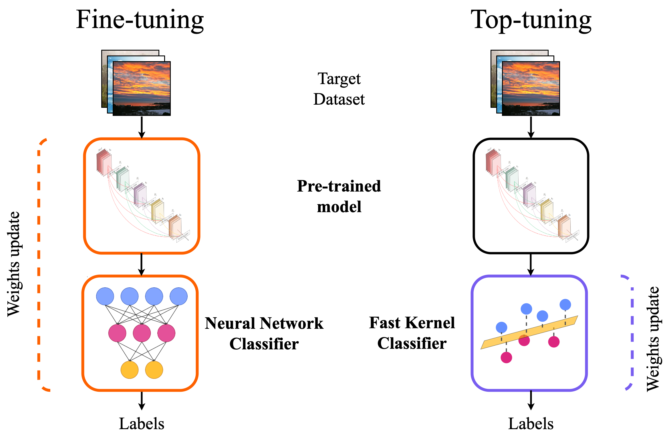
Figure 1: The two pipelines. (Left) The Fine-Tuning pipeline. All the model weights are updated. (Right) The Top-tuning pipeline. Only the fast kernel weights are updated.

Instead, in this paper we propose an approach whose goal is to exploit efficient kernel-based algorithms that are seldom applied to image classification: to compensate for their lack of representation capability, we adopt convolutional features[80] produced by a state-of-the-art model pre-trained on ImageNet [14], with no further tuning. These features are used as input to train a fast and scalable kernel classifier anew[78, 58]. This is a simple transfer approach[19, 36] aiming at exploiting knowledge from the pre-train source. We re-examine such methodology in terms of common practices for transfer learning combining deep nets and fast and scalable kernel methods.
We show that the adopted model, based on Nyström approach to reduce the problem size and on a preconditioned gradient solver for kernel methods, has a remarkable impact on training time and scalability. We refer to such approach as top-tuning and we show it in Figure 1(Right).

To investigate the common transfer learning scenario we focus on small to medium-size dataset, where transfer learning is more commonly applied. Although we do not focus on a specific application, we show that top-tuning methodology can be particularly effective when data availability is limited and fast training is relevant. This is typical of robotics devices and autonomous systems, especially when operating in unconstrained, quickly changing scenarios, where multiple training may need to be done on the fly[52, 70]. Our study shows that top-tuning is a promising alternative to fine-tuning for small-medium-sized datasets. Indeed, top-tuning provides comparable accuracy with respect to fine-tuning , with training times between one and two orders of magnitude smaller.

More in detail, to assess the potential of the proposed methodology, in our study we focus on three different aspects: (a) Target dataset: to ensure the generality of our empirical observations, we consider 32 small to medium-sized target datasets, showing that the top-tuning approach is $\simeq 85$ times faster on average with respect to the fine-tuning one. To provide more robust results we confirm our findings with two additional head classifiers: a naive shallow net and a ridge regressor, showing a smaller still significant speed-up. (b) Pre-trained model: to evaluate the influence of the specific pre-trained model, we include seven different state-of-the-art pre-trained models. We consider complex architectures such as Xception and Vision Transformers, as well as smaller models for embedded devices such as MobileNetV2. Our findings are confirmed showing that despite different pre-trained models, the top-tuning approach is $\simeq 70$ times faster on average with respect to the fine-tuning one. (c) Pre-training dataset: to assess dependency on the source dataset, we consider four distinct datasets for pre-training, taking into account different factors such as the amount of images and classes, and image size. We show the influence of the pre-training dataset on the downstream task, identifying the number of classes as a crucial factor in the pre-training dataset.

The main contributions of this work are: (1) A systematic empirical study on training time efficiency involving 3500 training processes, comparing top-tuning and fine-tuning approaches on a large ensemble of small to medium size datasets. (2) An evaluation of a fast kernel classifier method based on the Nyström approximation when coupled with pre-trained features, showing its potential wide applicability to the image domain and its effectiveness in general-purpose computer vision scenarios. (3) An analysis of the effectiveness of pre-training quality, which prioritizes the number of classes to the number of samples.

The rest of the paper is organized as follows: section 2 presents an account of the relevant background while section 3 reports details on our methodology. In section 4 we present the hyper-parameters configuration and we provide details on the datasets involved in the experiments. In section 5, we illustrate the results of our empirical analysis. Finally, section 7 is left to concluding remarks.

2 Related works

In the last few years, different papers focused on the importance of convolutional features. For instance, in [19] the authors analyze how convolutional networks behave as feature extractors. An in-depth analysis is provided on the importance of low, middle, and high-level convolutional features. In [80] the effectiveness of CNN features is tested on a series of experiments conducted on recognition tasks. In [36] different classification algorithms are tested on image features extracted via a convolutional neural network. Moreover, recent papers focus on the properties of specific neural network architectures on transfer-learning accuracy. In [41], the authors evaluate if models that exhibit superior performance while being trained on ImageNet also display better performance in other visual tasks. They show that model accuracy on ImageNet strongly correlates with the performances of the same model on target tasks except for fine-grained image datasets, where pretraining on ImageNet provides minimal benefits.

To assess the importance of the ImageNet pre-train, recent works focused on ImageNet factors that contribute to the superior descriptive abilities of pre-trained models’ learned features. In [32] the authors perform an empirical investigation on ImageNet properties, training a CNN on different subsets of ImageNet, varying the number of samples, classes, and granularity to assess their effect in terms of accuracy.

Several works focus on the problem of speeding up the training process, evaluating potential influencing factors, and proposing faster training strategies. In [34] the authors propose a method to significantly reduce the training cost of a transformer-based model, by updating only a limited portion of the weights. In [51] a parameter-efficient method is proposed based on scaling and shifting deep features extracted from a pre-trained model. In [26] the authors present a unified framework that establishes connections between the design of state-of-the-art parameter-efficient methods. In [27] the authors focus on the impact of a CNN complexity on the training time, evaluating the accuracy with constrained time cost, considering the influence of different factors including depth, number of filters, and filter size. In [40], the authors investigate the paradigm of pre-training deep models on large supervised datasets in a transfer-learning framework for different vision tasks. They introduce a fine-tuning protocol that avoids expensive hyperparameters search, which is replaced by a custom heuristic procedure. Despite the recent attempts to reduce the costs associated with training procedures, the average number of parameters of the referenced models ranges from $10^{5}$ to $10^{8}$. Our approach, instead, usually involves $10^{4}$ training parameters, a number that is one order of magnitude smaller than the most efficient referenced fine-tuning protocol, and up to four orders of magnitude smaller than the others.

Moreover, different strategies to reduce training and inference time for CNNs are proposed, including the combination of simplified convolutional filters[54] or the use of one-dimensional filters[35]. Another relevant area of research includes the compression of deep neural networks[9] to reduce their storage and computational inference cost. This research field focuses on different approaches such as parameters pruning[76] and quantization[21], aiming at decreasing the time the model needs to make a prediction. Indeed such techniques can be particularly useful to reduce computational costs at test time.

Nonetheless, the aforementioned works focus on strategies to reduce training or inference time, with no specific comparison between different approaches nor evaluating the trade-off between accuracy and training resources. In this paper, instead, we perform an extensive training time and accuracy analysis, comparing different top-tuning and fine-tuning approaches on a large ensemble from small to medium size datasets, a relevant regime for transfer learning problems. We show that convolution features pre-trained on rich datasets such as ImageNet, provide general-purpose representation which can be transferred to a new task simply by training an external classifier. Such an approach shows a comparable accuracy with respect to fine-tuning, with a significant training process speed-up.
The speed-up we achieve is also boosted by the choice of a fast kernel method as a head classifier. In the last few years, the fast kernel approach we are adopting was tested in different scenarios. In [58, 61] theoretical guarantees for the Nyström approximation technique are provided and empirically examined. Its effectiveness in terms of speed is shown in classical numerical feature datasets, not with computer vision datasets. In [52, 6] the fast kernel is tested on specific robotic datasets for detection and pose-estimation tasks. In [3, 56] Nyström approximation is tested on basic image datasets such as MNIST and CIFAR10 while in [94] it is used for 3D surface reconstruction. In our work we instead present an extensive analysis of more than thirty general-purpose image datasets, proving the effectiveness of the fast kernel approach on a wide set of image classification tasks, and showing its potential in the computer vision domain.

3 Theory

We assume we are given a state-of-the-art deep learning model pre-trained on a source dataset (e.g. ImageNet), and a target dataset of input-output pairs $\{(x_{i},y_{i})\}_{i=1}^{n}$ to address a new image classification problem. The inputs images, the outputs are discrete labels $y_{i}\in\{1,\dots,T\}$, for instance different semantic classes. In our study, we consider two alternative transfer approaches, with the aim of highlighting the potential of our top-tuning methodology versus the common fine-tuning alternative:

1. Fine-tuning: a typical deep learning architecture for image classification, includes $C$ convolutional layers followed by L fully connected layers, which we may formalize as:

   $$\Phi_{FT}=\underbrace{\Phi_{C+L}\circ\ldots\Phi_{C+1}}_{\text{Fully connected layers}}\ \circ\underbrace{\Phi_{C}\circ\ldots\circ\Phi_{1}(x)}_{\text{Convolutional layers}}.$$ (1)

   In the basic idea of transfer learning by fine-tuning, we start from a pre-trained model $\Phi_{PT}$ and update the structure of the fully connected layers to address the new classification task. Then we fine-tune the model on the target dataset. Notice that this procedure may involve both the parameters of the fully connected and of the convolutional layers in an end-to-end fashion minimizing an empirical error via back-propagation. It can be more or less deep, depending on the portion of the architecture we want to fine-tune. The fine-tuning pipeline is shown in Figure 1(Left).

2. Top-tuning: in this case, we start from a pre-trained model as in Equation 1; we fix the convolutional layers $\Phi_{C},\ldots,\Phi_{1}$. We then compute the pre-trained convolutional features on the target dataset and use them to train a fast kernel classifier. The overall top-tuning pipeline is shown in Figure 1(Right), and may be formalized as follows:

   $$\Phi_{TT}=\underbrace{\Psi}_{\text{Kernel feature map}}\circ\underbrace{\Phi_{C}\circ\ldots\circ\Phi_{1}(x)}_{\text{Convolutional layers}}.$$ (2)

   $\Psi$ is a typically infinite-dimensional feature map corresponding to a kernel $k(z,z^{\prime})$, where $z$ and $z^{\prime}$ are feature vectors composed by the pre-trained convolutional features computed as

   $$z=\Phi_{C}\circ\ldots\circ\Phi_{1}(x).$$

   Such features are assumed to be fixed and are not trained/tuned. Therefore, the only free parameters $W$ are computed by a ridge regression minimizing

   $$\hat{f}(z)=\min_{W}\sum_{i=1}^{n}\|Wz_{i}-\mathbf{y}_{i}\|^{2}+\lambda\|W\|_{F}^{2}$$ (3)

   where $\|\cdot\|_{F}$ is the Frobenious norm, $\lambda$ is a regularization parameter controlling the complexity of the solution. Using the representer theorem [79] Equation 3 can be re-written as

   $$f(z)=W\Phi(z)=\sum_{i=1}^{n}k(z,z_{i})\boldsymbol{\alpha}_{i},\qquad\boldsymbol{\alpha}_{i}\in\mathbb{R}^{T},$$ (4)

   where the coefficients $\alpha_{i}$ satisfy the linear system

   $$(\mathbf{K}+\lambda I)\boldsymbol{\alpha}=\mathbf{Y},$$ (5)

   with $\boldsymbol{\alpha}=(\boldsymbol{\alpha}_{1},\dots,\boldsymbol{\alpha}_{n}),\mathbf{Y}=(\mathbf{y}_{1},\dots,\mathbf{y}_{n})\in\mathbb{R}^{nT},$ and $\mathbf{K}\in\mathbb{R}^{nT}$ with $\mathbf{K}_{ij}=k(x_{i},x_{j})$. The solution can be determined as

   $$\boldsymbol{\alpha}=(\mathbf{K}+\lambda\mathbf{I})^{-1}\mathbf{y}.$$ (6)

   Equation 6 requires inverting an $n\times n$ matrix, with $n$ training samples; this operation cost $\mathcal{O}(n^{3})$ in time and $\mathcal{O}(n^{2})$ in space. To make the kernel ridge classifier significantly faster and more efficient, we rely on Nyström approximation[64] that solves the same problem in a smaller space. Therefore we consider a reduced set of $m$ inducing points taken among the $n$ of the training set. By taking $m=\mathcal{O}(\sqrt{n})$ we have strong theoretical guarantees and empirical evidence that the error does not increase and leads to computational cost reduction. The time cost is reduced to $\mathcal{O}(n\ log(n)\ \sqrt{n})$. The space needed also decreases to $\mathcal{O}(n)$. More details about this procedure can be found in[78, 58].

4 Material and methods

In this section, we present technical details about the conducted experiments, to allow the work to be reproduced by an independent researcher. First, we consider the hyper-parameters tuning, both for the fine-tuning and top-tuning procedures. Then we report details about the datasets used in the empirical analysis.

4.1 Hyper-parameters tuning

A model can be tuned in several ways involving numerous hyper-parameters. In our analysis, we do not focus on an exhaustive hyper-parameters exploration. Instead, we consider a set of plausible configurations, both for the fine-tuning and the top-tuning pipelines, according to guidelines in previous works. It is worth noticing that, for each pipeline, the overall training time is computed as the summation of every considered configuration training time.

Fine-tuning hyper-parameters:
We perform a five-fold cross-validation analysis involving the following hyper-parameters:

• Training steps: inspired by previous studies on a similar context[41] we limited this quantity to 20.000 training steps, coupled with an early stopping criterion.

• Early stopping: we monitor the validation loss with a patience parameter equal to $10$.

• Weights update: we only consider fine-tuning the whole convolutional part, making the model more adaptable to the downstream task with respect to the top-tuning approach. That is to avoid a combinatorial explosion in the number of configurations, that would result in excessive and unfair training time for the fine-tuning pipeline.

• Batch size: taking into account previous studies about batch size[25, 55, 4] we compute it as: $b=\lfloor 2^{2\cdot log_{10}(n)-1}\rfloor$ where $n$ is the number of points in the dataset.

• Optimizer: we use default Stochastic Gradient Descent (SGD). As suggested by[22], we use two different learning rates: $l=\{0.1,0.01\}$

Overall, we run two training configurations for every fold, one for each considered learning rate value as all the remaining hyper-parameters are fixed. To evaluate the accuracy, we consider the best-performing configuration. Training time is the sum of the training times requested for both configurations.

Top-tuning hyper-parameters:
Also for the top-tuning approach, we perform a five-fold cross-validation analysis involving the following hyper-parameters:

• Kernel: the approximated kernel ridge regression is based on a Gaussian kernel $k(z,z^{\prime})=e^{-\frac{\|z-z^{\prime}\|^{2}}{2\gamma^{2}}}$, with $\gamma$ kernel width. We use two values of $\gamma=\{10^{2},10^{3}\}$.

• Regularization: we consider two values for the regularization term: $\lambda=\{10^{-5},10^{-6}\}$

Overall, we run four training configurations for every fold, as two values for both kernel width and regularization are tested. To evaluate the accuracy, we consider the best-performing configuration. Training time is the sum of the training times requested for the four configurations.
The described hyperparameter tuning procedure is based on a coarse grid search. This allows us to perform a fair comparison with fine-tuning approaches, where the number of hyperparameters is much larger. However, as an alternative, it is possible to exploit automatic hyperparameter optimization procedures for fast-kernel approaches, as the one outlined in [57], developed for Nyström approximation methods.

4.2 Datasets details

Dataset name	#images (Tr/Te)	Img. size mean	#classes
AFHQ (AF)[10]	13.167/1.463	$512\times 512$	3
Beans (BE)[46]	1.167/128	$500\times 500$	3
Best artworks (BA)[7]	7.896/878	$980\times 921$	50
Boat types (BT)[13]	1.315/147	$905\times 1234$	9
Caltech-101 (C101)[18]	3.060/6.084	$251\times 282$	102
Cassava (CSV)[62]	7.545/1.885	$573\times 611$	5
Cats vs Dogs (CVSD) [17]	20.935/2.327	$365\times 410$	2
Chest xray (CXRAY) [38]	4.708/524	$968\times 1321$	2
CIFAR10 (CIF10) [43]	50.000/10.000	$32\times 32$	10
CIFAR100 (CIF100) [43]	50.000/10.000	$32\times 32$	100
Citrus leaves (CLV) [74]	534/60	$256\times 256$	4
Colorectal hist (COL) [37]	4.500/500	$150\times 150$	8
Deep weeds (DW) [65]	15.758/1.751	$256\times 256$	9
DTD (DTD)[12]	3.760/1.880	$453\times 500$	47
EuroSAT (ES) [29]	24.300/2.700	$64\times 64$	10
FGVC Aircraft (AIR)[53]	6.667/3.333	$353\times 1056$	100
Footb vs Rugby (FVSR) [20]	2.203/245	$618\times 788$	2
Gemstones (GEM) [8]	2.571/286	$330\times 335$	87
Hors or Hum (HVSH) [60]	1.027/256	$300\times 300$	2
iCubWorld subset (ICUB)[70]	86.400/9.600	$256\times 256$	10
Indian Food (IF) [72]	3.600/400	$550\times 610$	80
Make No Make(MVSN)[85]	1.355/151	$211\times 246$	2
Malaria (MAL) [73]	24.802/2.756	$133\times 132$	2
Meat quality (MQA) [90]	1.706/190	$720\times 1280$	2
Oxford Flowers (OF) [63]	2.040/6.149	$538\times 624$	102
Oxford-IIIT Pets (OP) [69]	3.680/3.669	$383\times 431$	37
Plankton (PL) [71]	4.500/500	$106\times 120$	10
Sars Covid (SCOV) [82]	2.232/249	$260\times 350$	2
Stanford Cars (SC) [42]	8.144/8.041	$308\times 573$	196
Stanford Dogs (SD) [39]	12.000/8.580	$386\times 443$	120
Tensorflow Flowers(TFF) [89]	3.303/367	$272\times 365$	5
Weather (MW) [83]	1.012/113	$335\times 506$	4

Table 1: The datasets adopted in our analysis. For every dataset, we provide the number of images (train and test split, respectively), the mean image size of the dataset, and the number of classes.

We include 32 small to medium-sized datasets in our experiments, from a wide range of contexts and scenarios (see Table 1). Our collection includes popular datasets in the computer vision community, like CIFAR10/100 and Caltech101, as well as more challenging datasets where the amount of data is limited with respect to the number of classes and complexity of the task (e.g., Stanford Cars and FGVC aircraft). Finally, we include datasets with a significantly limited amount of images, to consider practical cases where transfer learning procedures may be fundamental (e.g., Beans and Citrus leaves). Indeed, we did not include large datasets in our analysis since the transfer learning technique is generally not crucial in contexts where there is data abundance. From Table 1 we can notice that both numbers of images and classes can vary deeply from one task to another. This can influence the task’s hardness. On average each dataset has $11746.46$ images and $35.21$ classes. The average number of images per class is $1780.24$ The dataset with the most images per class is the Malaria dataset with 12401 images per class. The dataset with few images per class is Oxford Flowers with 20 images per class.

5 Results

We now describe the details of the empirical analysis. Firstly, we conduct a comparison between fine-tuning and top-tuning, focusing on accuracy and training time. Then, to ensure robustness in our findings, we substitute the fast-kernel head classifier with a vanilla fully connected network or a ridge regressor. Later, to assess the impact of the pre-trained architecture on the results, we explore seven different pre-trained neural networks as potential replacements for the backbone used in both fine-tuning and top-tuning approaches. Lastly, we evaluate the significance of the pre-trained source data by considering four different datasets for pre-training the convolutional backbone used in both fine-tuning and top-tuning. All the experiments have been carried out on a single Quadro RTX 6000 GPU, 24Gb VRAM.

5.1 Top-tuning is highly faster with limited accuracy drop

To compare fine-tuning and top-tuning approaches, we first fix the neural network model and the pre-training dataset, considering an ImageNet pre-trained DenseNet201[31] architecture. This model represents a good compromise between predictive power and size, in terms of the number of parameters. We consider the 6 different configurations defined in subsection 4.1 averaging the results of a 5-folded procedure over the 32 datasets, resulting in $6\cdot 5\cdot 32=960$ distinct training processes.

Figure 2: Overall speed-up on different target datasets obtained by the top-tuning model with respect to the fine-tuning one. Each column represents a dataset. The corresponding height represents the speed-up factor of the top-tuning model with respect to the fine-tuning one(e.g. on the AFHQ dataset the top-tuning training was $\sim 95$ times faster). All the experiments have been carried out on a single Quadro RTX 6000 GPU, 24Gb VRAM.

In Figure 2 we show the overall results in terms of training time speed-up. Each column refers to a different dataset, reporting the speed-up $SpUp$ obtained by the top-tuning with respect to fine-tuning. The top-tuning model is always highly faster to train than the fine-tuning one. Indeed, given the fine-tuning training time $t_{\text{fine-tuning}}$ and the top-tuning training time $t_{\text{top-tuning}}$,

$$SpUp=\dfrac{t_{\text{fine-tuning}}}{t_{\text{top-tuning}}}$$

is in the range $[10,165]$, with the top-tuning model being between 10 and 165 times faster to train. The average speed-up is $84.64\pm 38.97$ across the datasets. On larger datasets, e.g. CIFAR100, the training time was reduced from $\sim 2$ hours to $\sim 10$ minutes; computed as the training time sum of the two fine-tuning and four top-tuning configurations, respectively.

We can relate the faster training time to: (i) number of parameters: the top-tuning model has a number of parameters on average two orders of magnitude lower than the fine-tuning ones. Indeed, a fully tunable convolutional model like DenseNet contains more than 20 million learnable parameters. Instead, the top-tuning model is made by a few dozen thousand parameters (ii) impact of backpropagation: every layer needs to wait for the subsequent layer computation.

To show that training time speed-up does not affect accuracy, in Figure 3 we report the overall accuracy results. Each point represents a different dataset. Its position is given by the accuracy obtained by the best fine-tuning configuration on the x-axis, and by the best top-tuning configuration on the y-axis. The diagonal is marked for readability purposes. Intuitively, when a point is lying below the diagonal, the fine-tuning model is performing better w.r.t the top-tuning one, and vice-versa.

Figure 3: Overall accuracies on different target datasets. Each point represents a dataset. The accuracy obtained by the best fine-tuning model is shown on the x-axis. The best top-tuning model accuracy is shown on the y-axis. When a point is lying below the diagonal, the fine-tuning model is performing better w.r.t the top-tuning one, and vice-versa.

Most of the datasets lie around the diagonal, showing similar accuracy between fine-tuning and top-tuning methods. Indeed,

$$\Delta Acc=Acc_{\mathrm{top-tuning}}-Acc_{\mathrm{fine-tuning}}$$

is in the range $[-2.5\%,+2.5\%]$ in $60\%$ of our experiments. Only on a few datasets, e.g. FGVC aircraft and Stanford Cars(SC), fine-tuning provides a benefit. This behavior could be related to two factors. (i) Representation in ImageNet: as pointed out by [41], in ImageNet cars and planes are represented at a coarse-grained level. For instance, ImageNet contains only two plane classes; (ii) Dataset hardness in terms of the number of classes, granularity, and the number of images per class.

Dataset	$\Delta$Acc$\uparrow$	SpUp$\uparrow$
AFHQ	$+0.10\%$	$94.70\times$
Beans	$+0.90\%$	$116.3\times$
Best artworks	$+3.10\%$	$65.90\times$
Boat types	$+0.50\%$	$131.5\times$
Caltech-101	$+1.10\%$	$94.00\times$
Cassava	$-4.50\%$	$44.00\times$
Cats vs Dogs	$-0.20\%$	$60.00\times$
Chest xray	$+0.50\%$	$62.40\times$
CIFAR10	$-2.80\%$	$28.90\times$
CIFAR100	$-3.70\%$	$12.10\times$
Citrus leaves	$+7.30\%$	$109.5\times$
Colorect. histology	$+0.50\%$	$89.20\times$
Deep weeds	$-9.10\%$	$57.70\times$
DTD	$+2.90\%$	$82.80\times$
EuroSAT	$-2.40\%$	$39.10\times$
FGVC Aircraft	$-10.6\%$	$60.90\times$

Dataset	$\Delta$Acc$\uparrow$	SpUp$\uparrow$
Football vs Rugby	$+1.90\%$	$124.8\times$
Gemstones	$-0.20\%$	$147.6\times$
Horses or Humans	$+5.20\%$	$131.3\times$
iCub World subset	$-1.00\%$	$32.60\times$
Indian Food	$-1.10\%$	$122.6\times$
Make up	$+1.70\%$	$102.5\times$
Malaria	$-2.00\%$	$46.80\times$
Meat Quality	$+0.00\%$	$163.6\times$
Oxford Flowers102	$+4.50\%$	$96.30\times$
Oxford-IIIT Pets	$+4.50\%$	$94.60\times$
Plankton	$+0.00\%$	$75.50\times$
Sars Covid	$-0.40\%$	$107.0\times$
Stanford Cars	$-15.7\%$	$76.90\times$
Stanford Dogs	$+5.20\%$	$22.50\times$
Tensorflow flowers	$-1.40\%$	$62.40\times$
Weather	$+0.90\%$	$152.4\times$

Table 2: Quantitative results about the analysis on different datasets. The second column reports the $\Delta Acc=Acc_{\mathrm{top-tuning}}-Acc_{\mathrm{fine-tuning}}$. The third one refers to the corresponding speed-up obtained when using the top-tuning procedure(e.g. on the AFHQ dataset the top-tuning training was $94.70$ times faster).

Table 2 summarizes the quantitative results obtained with our experiments both in terms of accuracy and training time speed-up. For every dataset, we report the $\Delta Acc$ and the corresponding speed-up $SpUp$.
Lastly, although in this work we do not focus on inference time, we report for completeness that the two pipelines needed similar time for a prediction.

5.2 Analysis with different head classifiers

To test the generality of our approach we replace the fast kernel classifier with two head classifiers: a shallow net and a ridge regression classifier. The training procedure is similar to the one presented in section 3. For the shallow net, we consider just two configurations with default Stochastic Gradient Descent (SGD) and two different learning rates: $l=\{0.1,0.01\}$. The training time reported in the results is the sum of the computational time required for the two training instances. Notice that this architecture is identical to the fine-tuning one. The main difference lies in which part of the model is tuned. The shallow nets update only the parameters of the last three fully connected layers while the fine-tuning one update all the weights of the model.

For the Ridge regressor, we use three different configurations corresponding to three different values of the regularization term $\alpha=\{10^{1},10^{-1},10^{-3}\}$. Here again, the training time reported in the results is the sum of the computational time required for the three training instances.

In Figure 4 we compare, in terms of training time, the fine-tuning model with both the shallow net(left) and the ridge regressor(right) as an external classifier. With the fast kernel classifier as an external classifier, the average speed-up is $84.64\pm 38.97$. Instead, by using a shallow net as an external classifier we obtain an average speedup of $40.74\pm 12.43$. The speed-up is instead $16.37\pm 9.57$ if we use the ridge regressor as an external classifier.

These results show that, regardless of the choice of external classifier, top-tuning confirms a training time speed-up of at least one order of magnitude with respect to the fine-tuning pipeline. Among them, the fast-kernel model reports a significant boost with respect to to its competitors.

Figure 4: Overall speed-up results on different target datasets with shallow net and ridge as external classifiers w.r.t the fine-tuning model. (Left) Speed-up obtained over different target datasets by using a shallow net as an external classifier. (Right) Speed-up obtained over different target datasets by using a ridge regressor as an external classifier.

In Figure 5 we compare, in terms of accuracy, the fine-tuning model with both the shallow net(left) and the ridge regressor(right) as external classifiers. The obtained results are similar to the ones shown in Figure 2. Most of the datasets lie around the diagonal for both shallow net and ridge as an external classifier, showing similar accuracy between fine-tuning and top-tuning methods, confirming the findings of subsection 5.1.

Figure 5: Overall accuracy results on different target datasets with shallow net and ridge as external classifiers w.r.t the fine-tuning model. (Left) Accuracies obtained over different target datasets by using a shallow net as an external classifier. (Right) Accuracies obtained over different target datasets by using a ridge regressor as an external classifier.

5.3 Impact of pre-trained model

To weight the dependency of the results on the pre-trained architecture we extend the results obtained with DenseNet201 on five state-of-the-art pre-trained models: (i) EfficientNetB0 [88]; (ii) InceptionResNetV2 [86]; (iii) MobileNetV2[30]; (iv) ResNet152[28]; (v) Xception[11].
We test these models on four different datasets where: fine-tuning has only marginal benefits (Caltech-101, CIFAR100), top-tuning approach provides better results with respect to fine-tuning (DTD), and fine-tuning outperforms top-tuning approach (Stanford Cars).
The training procedure is analogous to the one performed for DenseNet201 with 5 additional pre-trained models and a subset of 4 datasets, performing 600 additional training processes.
In Figure 6 we show the overall results. Each color refers to a different target dataset, each symbol corresponds to a different pre-trained neural network.

Figure 6: Overall results on different pre-trained models. (Left) Accuracies over different target datasets with different pre-trained models. (Right) Speed-up obtained by the top-tuning model w.r.t the fine-tuning one for each dataset and for each pre-trained model.

	Caltech-101		CIFAR100		DTD		Stanford Cars
	$\Delta$Acc$\uparrow$	SpUp$\uparrow$	$\Delta$Acc$\uparrow$	SpUp$\uparrow$	$\Delta$Acc$\uparrow$	SpUp$\uparrow$	$\Delta$Acc$\uparrow$	SpUp$\uparrow$
DenseN201	$+1.10\%$	$94.00$	$-3.70\%$	$12.1$	$+2.90\%$	$82.80$	$-15.7\%$	$76.90$
Eff.NB0	$-5.60\%$	$109.3$	$-12.1\%$	$8.70$	$-2.60\%$	$76.80$	$-21.9\%$	$73.40$
Inc.R.NV2	$-2.80\%$	$85.10$	$-11.1\%$	$10.2$	$-1.50\%$	$126.3$	$-18.3\%$	$137.6$
MobileNV2	$+14.3\%$	$39.40$	$+0.10\%$	$7.90$	$+23.5\%$	$89.80$	$-4.3\%$	$48.10$
ResN152	$+2.90\%$	$82.60$	$-5.10\%$	$13.7$	$+2.90\%$	$150.2$	$+7.2\%$	$78.90$
Xception	$-4.00\%$	$67.10$	$-15.4\%$	$10.3$	$-3.90\%$	$81.00$	$-22.7\%$	$98.10$

Table 3: Analysis on different pre-trained models: variation in accuracy ($\Delta$Acc) and speedup (SpUp), between fine-tuning and top-tuning.

Different pre-trained neural networks show a similar trend to the one obtained by DenseNet201. Figure 6(Left) shows that on datasets where the drop between fine-tuning and top-tuning was marginal (e.g. Caltech, DTD) using different pre-trained model results in an analogous behavior. Similarly, on a dataset where such the drop was greater (e.g. Stanford Cars) using different pre-trained results in a similar performance deterioration. Figure 6(Right) confirms our findings on the matter of training time speedup, showing that the top-tuning approach is highly faster with respect to the fine-tuning one. Table 3 summarizes the results obtained both in terms of accuracy and training time speed-up. It shows quantitatively that different pre-trained networks behave similarly on the same dataset with respect to DenseNet201. Moreover, it shows that the top-tuning approach is approximately 70 times faster with respect to the fine-tuning one. Such results suggest that our findings are low dependent on the pre-trained neural network adopted.

Results with different fine-tuning configurations

We further evaluate different protocols of fine-tuning, to investigate the impact of such protocols on training time and test accuracy. In the new set of experiments, we explore intermediate fine-tuning configurations, considering our best-performing pre-trained convolutional model, DenseNet201, which consists of 5 dense blocks in its convolutional part. Thus, we compare three partial fine-tuning protocols:

• Updating the last two dense blocks of the convolutional part, which corresponds to updating 47.5% of the weights in the convolutional part.

• Updating the last four dense blocks of the convolutional part, which corresponds to updating 92.1% of the weights in the convolutional part.

• Updating all five dense blocks, which corresponds to updating 100% of the weights in the convolutional part. It is noteworthy that this scenario corresponds to the original fine-tuning configuration.

Figure 7: Overall results on different fine-tuning configurations. (Left) Speed-up obtained over different target datasets by the top-tuning model w.r.t different fine-tuning configurations (Right) Accuracies obtained over different target datasets with different partial fine-tuning configurations.

In Figure 7(Left), we present the speedup results. We compute the ratio between each intermediate fine-tuning configuration training time and top-tuning training time. As expected, the larger the updated portion of the convolutional part, the greater the cost of fine-tuning, resulting in a higher speed-up of the top-tuning approach.
In Figure 7(Right), we show the accuracy results for the different fine-tuning configurations. We can notice that, within the same dataset, there is no substantial difference in accuracy among the various configurations. These results seem to confirm that the ImageNet learned representation is very effective, suggesting that the top-tuning approach may be an efficient alternative to fine-tuning for the investigated datasets.

Results with transformers

In the last few years, a new generation of models called transformers, has been introduced. Such models are usually composed of hundreds of millions of parameters, obtaining state-of-the-art performances. Commonly, they are pre-trained on an extended version of ImageNet called ImageNet21k[77]. In the following experiments we replace the first convolutional part of the pipeline with a Vision Transformer(ViT-L/16) as presented in [16]. With 32 target datasets for the top-tuning approach and 2 target datasets for the fine-tuning one, we perform $650$ additional training processes.
For the top-tuning pipeline, we were able to replicate our analysis on all 32 target datasets. We report the results in Table 4, where $\Delta Acc=Acc_{\mathrm{Transform}}-Acc_{\mathrm{Conv}}$ is the accuracy gain of transformer with respect to DenseNet201. On average $\Delta Acc=4.58\%\pm 5.36\%$ shows good improvements by using the pre-trained transformer as a features extractor.

Dataset	$\Delta$Acc$\uparrow$
AFHQ	$-0.03\%$
Beans	$3.91\%$
Best art	$10.1\%$
Boat	$7.89\%$
Cal101	$1.78\%$
Cassava	$8.07\%$
Cat Do	$1.14\%$
Ch xra	$-0.65\%$

Dataset	$\Delta$Acc$\uparrow$
CIF10	$5.92\%$
CIF100	$14.56\%$
Citr lea	$2.67\%$
Col hist	$0.72\%$
Deep w	$11.1\%$
DTD	$9.98\%$
EuSAT	$0.87\%$
FG Air	$-9.40\%$

Dataset	$\Delta$Acc$\uparrow$
Foot Ru	$8.98\%$
Gemst	$6.08\%$
Hor Hu	$0.00\%$
iCub	$0.12\%$
Ind Fd	$13.0\%$
MkNoM	$7.02\%$
Malaria	$1.84\%$
Meat qu	$-0.63\%$

Dataset	$\Delta$Acc$\uparrow$
Oxf Flo	$12.0\%$
Oxf Pet	$5.75\%$
Plankt	$0.00\%$
Sa Cov	$-0.96\%$
St Cars	$4.72\%$
St Dog	$13.7\%$
Ten Fl	$6.98\%$
Weath	$-0.53\%$

Table 4: Analysis of the transformer model for the top-tuning pipeline. $\Delta Acc=Acc_{\mathrm{Transform}}-Acc_{\mathrm{Conv}}$ is the accuracy gain of transformer model with respect to convolutional model

For the fine-tuning approach, we decided not to replicate the analysis on all the datasets. Indeed, the duration of a single fine-tuning training process can extend for several hours, even on very small datasets. Therefore, to test our findings, we carried out the whole analysis on two datasets of modest size for the sake of comparison. We considered Citrus Leaves and Oxford Flowers, where we reached an absolute accuracy of $97.5\%$ and $99.1\%$, respectively. If we compare these values with the ones obtained by the top-tuning pipeline ($98.3\%$ and $99.5\%$, respectively) the results confirm the marginal accuracy benefits of fine-tuning a transformer model. On the training time, we obtain an even more remarkable speedup($226.19\times$ and $185.05\times$, respectively).

5.4 Pre-training dataset influence transfer’s effectiveness

We now explore the dependency of the results on the pre-training source dataset. To this purpose, we consider three alternative pre-training datasets:

• CIFAR100: we consider CIFAR100 as a simplified version of ImageNet. With this dataset, we test the impact of a reduced number of images, classes and image size.

• ImageNet100: we extract an ImageNet subset with the same number of images and classes of CIFAR100. To make this dataset as similar as possible to CIFAR100 in terms of label semantics: $75\%$ of labels selected from ImageNet are the same in CIFAR100, $15\%$ of them are similar and $10\%$ are different. With this dataset, we test the impact of image quality on the obtained results.

• ImageNet 50k: we extract an ImageNet subset that contains all the classes in ImageNet with the same number of data points contained in CIFAR100, that is 50k. The obtained dataset has 1000 classes with only 50 points per class. With this dataset, we test how the total number of classes affects the obtained results.

First, we train a DenseNet201 model from scratch on each of the three pre-training datasets. Then, we apply the two investigated pipelines as described in section 3 on five target datasets: one of the most difficult and one of the easiest datasets for both approaches (DTD and CIFAR10, respectively), one where top-tuning approach outperforms fine-tuning (Citrus Leaves) and the opposite case (Deep Weeds). Lastly, we consider the fine-grained Oxford Flowers 102. With five target datasets and three different pre-training, we perform 450 additional training instances.

Figure 8: Overall results on different pre-trains. For each target dataset, each color represents one of the four different pre-trains datasets. (Left) Accuracies obtained by top-tuning approach (Right) Accuracies obtained by fine-tuning approach.

		CIFAR10	Citrus Leaves	Deep Weeds	DTD	Oxf Flow
Top-Tun.	CIFAR100	$\bm{7.30\%}$	$4.7\%$	$15.2\%$	$26.3\%$	$24.0\%$
	ImageNet100	$16.8\%$	$6.7\%$	$11.1\%$	$22.0\%$	$24.3\%$
	ImageNet 50k	$12.7\%$	$\bm{1.0\%}$	$\bm{5.70\%}$	$\bm{17.5\%}$	$\bm{13.9\%}$
Fine-Tun.	CIFAR100	$\bm{4.9\%}$	$0.0\%$	$10.9\%$	$18.3\%$	$\bm{12.6\%}$
	ImageNet100	$6.3\%$	$\bm{-0.6\%}$	$6.7\%$	$\bm{13.0\%}$	$13.0\%$
	ImageNet 50k	$5.3\%$	$1.7\%$	$\bm{5.5\%}$	$13.1\%$	$16.7\%$

Table 5: Accuracy drops for pre-training alternatives to ImageNet. Each column represents a different target dataset, and each row is a different pre-train source. The reported value corresponds to the accuracy drop with respect to the original ImageNet pre-training. The lower the value, the better.

Figure 8(Left) refers to top-tuning accuracy for each pre-train. ImageNet pre-training brings the best results on the target datasets. ImageNet 50k is the best alternative, suggesting that the number of classes for the pre-training dataset has a great impact on the top-tuning approach. The only exception corresponds to CIFAR10, where CIFAR100 corresponds to the best pre-train. This behavior depends on CIFAR10 being de facto a CIFAR100 subset.

Figure 8(Right) refers to fine-tuning accuracy for each pre-train. ImageNet pre-training corresponds to the best accuracy. The difference between the other pre-training configurations is marginal. This is probably due to the fine-tuning training procedure, which mitigates the weight of different pre-training. Table 5 summarizes the quantitative results in terms of accuracy drop with respect to the original ImageNet pre-training.

6 Discussion

In the previous section, we present results describing the efficiency of an approach named top-tuning, for image classification tasks. We show that, with respect to conventional fine-tuning procedure, the top-tuning method is between 10 and 165 times faster to be trained, with either an absent or marginal accuracy drop.
The results obtained in this study pave the way for further developments.
Primarily, it is worth noticing that all the presented results exclusively pertain to the resolution of image classification problems. This task, although important, represents only a part of the topics addressed within the computer vision research field. An interesting development could evaluate the aforementioned techniques’ applicability to tasks requiring more structural understanding, such as detection or segmentation. Another potential extension could explore the effectiveness of top-tuning on video-related problems. Indeed, from this perspective, we are currently working on extending the top-tuning pipeline to the field of video action recognition, where efficiency is vital due to the large amount of data involved in video analysis. An additional extension could concern the automatic hyperparameters setting within the top-tuning method. We perform experiments exploiting an automatic hyper-parameter optimization procedure. The resulting accuracy is generally lower with respect to the grid search adopted in this work. This is probably due to the high dimensionality of the data compared to the usual regime for fast-kernel methods optimization, which is typically low-dimensional, leaving room for potential developments. In this regard, we are working to enhance the efficacy of the automatic procedure, with the aim of making the use of the top-tuning approach even more effective.
Secondly, we identify conditions where the top-tuning in its present formulation is less effective in terms of accuracy. This occurs when the target dataset simultaneously exhibits the following characteristics: it is underrepresented in the source dataset, it is of small size, and it is fine-grained. However, based on our experiments, this situation occurs rarely, as the aforementioned criteria are quite strong to satisfy at the same time. Moreover, despite a major accuracy drop, the top-tuning approach is still massively faster which can be the most crucial aspect. Finally, it is worth noting that even the fine-tuning procedure for fine-grained cases may lead to suboptimal results, as handling fine-grained data may require the use of appropriate strategies aimed at highlighting minimal differences between distinct classes.

7 Conclusions

The need for efficiency has become central in the context of deep learning, where complex models are trained with increasingly large datasets. In this work, we compare two popular transfer learning solutions in terms of training time and accuracy. The first one consists in fine-tuning a model pre-trained on a large source dataset. This approach may require significant computational resources, in terms of training time, GPU-CPU involvement, and memory usage. This is due to back-propagation and the potentially huge amount of parameters involved. An alternative solution consists in adopting a pre-trained model as-it-is as a features extractor, coupling it with an external head classifier, which we refer to as top-tuning
In this paper, we discuss the benefits of this alternative, in particular when a fast kernel head classifier is adopted. To support our claim, we reported an extensive experimental analysis involving 32 small to medium-sized target datasets through 3460 distinct training processes. Our experiments confirm that the top-tuning approach leads to a huge reduction in terms of training time, even from hours to a few minutes in different scenarios. Furthermore, fine-tuning has only marginal accuracy benefits with respect to the top-tuning approach. Indeed, in 60$\%$ of our experiments, $\Delta$Acc between fine-tuning and top-tuning is in range $[-2.5\%,+2.5\%]$. Moreover, our results showed that the marginal benefit of fine-tuning is low dependent on the neural network architecture used as a pre-trained model.
Another noteworthy aspect of this research is the demonstration of the efficacy of the Nyström approximated kernel method, which the top-tuning model relies on. Indeed, when combined with meaningful pre-trained features, we show its wide applicability to the domain of image classification.
Finally, by considering alternative pre-training datasets, in this paper we emphasize the importance of semantic diversity, showing that greater variability in the source data can have a significant impact on the target task.

References

- [1] Ulysse Côté Allard, François Nougarou, Cheikh Latyr Fall, Philippe Giguère, Clément Gosselin, François Laviolette, and Benoit Gosselin. A convolutional neural network for robotic arm guidance using semg based frequency-features. In 2016 IEEE/RSJ International Conference on Intelligent Robots and Systems (IROS), pages 2464–2470. IEEE, 2016.
- [2] Syed Muhammad Anwar, Muhammad Majid, Adnan Qayyum, Muhammad Awais, Majdi Alnowami, and Muhammad Khurram Khan. Medical image analysis using convolutional neural networks: a review. Journal of medical systems, 42(11):1–13, 2018.
- [3] Mikhail Belkin, Siyuan Ma, and Soumik Mandal. To understand deep learning we need to understand kernel learning. In International Conference on Machine Learning, pages 541–549. PMLR, 2018.
- [4] Yoshua Bengio. Practical recommendations for gradient-based training of deep architectures. In Neural networks: Tricks of the trade, pages 437–478. Springer, 2012.
- [5] Alfredo Canziani, Adam Paszke, and Eugenio Culurciello. An analysis of deep neural network models for practical applications. arXiv preprint arXiv:1605.07678, 2016.
- [6] Federico Ceola, Elisa Maiettini, Giulia Pasquale, Giacomo Meanti, Lorenzo Rosasco, and Lorenzo Natale. Learn fast, segment well: Fast object segmentation learning on the icub robot. IEEE Transactions on Robotics, 38(5):3154–3172, 2022.
- [7] Art challenge team. Best artworks of all time, feb 2019.
- [8] Daria Chemkaeva. Football vs rugby, mar 2020.
- [9] Yu Cheng, Duo Wang, Pan Zhou, and Tao Zhang. A survey of model compression and acceleration for deep neural networks. 2017.
- [10] Yunjey Choi, Youngjung Uh, Jaejun Yoo, and Jung-Woo Ha. Stargan v2: Diverse image synthesis for multiple domains. In Proceedings of the IEEE/CVF Conference on Computer Vision and Pattern Recognition (CVPR), June 2020.
- [11] François Chollet. Xception: Deep learning with depthwise separable convolutions. In Proceedings of the IEEE conference on computer vision and pattern recognition, pages 1251–1258, 2017.
- [12] M. Cimpoi, S. Maji, I. Kokkinos, S. Mohamed, , and A. Vedaldi. Describing textures in the wild. In Proceedings of the IEEE Conf. on Computer Vision and Pattern Recognition (CVPR), 2014.
- [13] Pierre-Alexandre Clorichel. Boat types recognition, nov 2018.
- [14] Jia Deng, Wei Dong, Richard Socher, Li-Jia Li, Kai Li, and Li Fei-Fei. Imagenet: A large-scale hierarchical image database. In 2009 IEEE conference on computer vision and pattern recognition, pages 248–255. Ieee, 2009.
- [15] Carl Doersch and Andrew Zisserman. Multi-task self-supervised visual learning. In Proceedings of the IEEE International Conference on Computer Vision, pages 2051–2060, 2017.
- [16] Alexey Dosovitskiy, Lucas Beyer, Alexander Kolesnikov, Dirk Weissenborn, Xiaohua Zhai, Thomas Unterthiner, Mostafa Dehghani, Matthias Minderer, Georg Heigold, Sylvain Gelly, et al. An image is worth 16x16 words: Transformers for image recognition at scale. In International Conference on Learning Representations, 2021.
- [17] Jeremy Elson, John (JD) Douceur, Jon Howell, and Jared Saul. Asirra: A captcha that exploits interest-aligned manual image categorization. In Proceedings of 14th ACM Conference on Computer and Communications Security (CCS). Association for Computing Machinery, Inc., October 2007.
- [18] Li Fei-Fei, Rob Fergus, and Pietro Perona. Learning generative visual models from few training examples: An incremental bayesian approach tested on 101 object categories. Computer Vision and Image Understanding, 106(1):59–70, April 2007.
- [19] Dario Garcia-Gasulla, Ferran Parés, Armand Vilalta, Jonatan Moreno, Eduard Ayguadé, Jesús Labarta, Ulises Cortés, and Toyotaro Suzumura. On the behavior of convolutional nets for feature extraction. Journal of Artificial Intelligence Research, 61:563–592, 2018.
- [20] Tanishq Gautam. Football vs rugby, mar 2021.
- [21] Amir Gholami, Sehoon Kim, Zhen Dong, Zhewei Yao, Michael W Mahoney, and Kurt Keutzer. A survey of quantization methods for efficient neural network inference. In Low-Power Computer Vision, pages 291–326. Chapman and Hall/CRC.
- [22] Ian Goodfellow, Yoshua Bengio, and Aaron Courville. Deep Learning. MIT Press, 2016.
- [23] Jiuxiang Gu, Zhenhua Wang, Jason Kuen, Lianyang Ma, Amir Shahroudy, Bing Shuai, Ting Liu, Xingxing Wang, Gang Wang, Jianfei Cai, et al. Recent advances in convolutional neural networks. Pattern Recognition, 77:354–377, 2018.
- [24] Dongyoon Han, Jiwhan Kim, and Junmo Kim. Deep pyramidal residual networks. In Proceedings of the IEEE conference on computer vision and pattern recognition, pages 5927–5935, 2017.
- [25] Fengxiang He, Tongliang Liu, and Dacheng Tao. Control batch size and learning rate to generalize well: Theoretical and empirical evidence. Advances in Neural Information Processing Systems, 32:1143–1152, 2019.
- [26] Junxian He, Chunting Zhou, Xuezhe Ma, Taylor Berg-Kirkpatrick, and Graham Neubig. Towards a unified view of parameter-efficient transfer learning. In International Conference on Learning Representations, 2021.
- [27] Kaiming He and Jian Sun. Convolutional neural networks at constrained time cost. In Proceedings of the IEEE conference on computer vision and pattern recognition, pages 5353–5360, 2015.
- [28] Kaiming He, Xiangyu Zhang, Shaoqing Ren, and Jian Sun. Deep residual learning for image recognition. In Proceedings of the IEEE conference on computer vision and pattern recognition, pages 770–778, 2016.
- [29] Patrick Helber, Benjamin Bischke, Andreas Dengel, and Damian Borth. Eurosat: A novel dataset and deep learning benchmark for land use and land cover classification. IEEE Journal of Selected Topics in Applied Earth Observations and Remote Sensing, 2019.
- [30] Andrew G. Howard, Menglong Zhu, Bo Chen, Dmitry Kalenichenko, Weijun Wang, Tobias Weyand, Marco Andreetto, and Hartwig Adam. Mobilenets: Efficient convolutional neural networks for mobile vision applications. CoRR, abs/1704.04861, 2017.
- [31] Gao Huang, Zhuang Liu, Laurens Van Der Maaten, and Kilian Q Weinberger. Densely connected convolutional networks. In Proceedings of the IEEE conference on computer vision and pattern recognition, pages 4700–4708, 2017.
- [32] Mi-Young Huh, Pulkit Agrawal, and Alexei A. Efros. What makes imagenet good for transfer learning? CoRR, abs/1608.08614, 2016.
- [33] Maxwell L. Hutchinson, Erin Antono, Brenna M. Gibbons, Sean Paradiso, Julia Ling, and Bryce Meredig. Overcoming data scarcity with transfer learning. CoRR, abs/1711.05099, 2017.
- [34] Menglin Jia, Luming Tang, Bor-Chun Chen, Claire Cardie, Serge Belongie, Bharath Hariharan, and Ser-Nam Lim. Visual prompt tuning. In European Conference on Computer Vision, pages 709–727. Springer, 2022.
- [35] Jonghoon Jin, Aysegul Dundar, and Eugenio Culurciello. Flattened convolutional neural networks for feedforward acceleration. In International Conference on Learning Representations Workshop, 2015.
- [36] Manjunath Jogin, Mohana, M S Madhulika, G D Divya, R K Meghana, and S Apoorva. Feature extraction using convolution neural networks (cnn) and deep learning. In 2018 3rd IEEE International Conference on Recent Trends in Electronics, Information Communication Technology (RTEICT), pages 2319–2323, 2018.
- [37] Jakob Nikolas Kather, Frank Gerrit Zöllner, Francesco Bianconi, Susanne M Melchers, Lothar R Schad, Timo Gaiser, Alexander Marx, and Cleo-Aron Weis. Collection of textures in colorectal cancer histology, 05 2016.
- [38] Daniel S Kermany, Michael Goldbaum, Wenjia Cai, Carolina CS Valentim, Huiying Liang, Sally L Baxter, Alex McKeown, Ge Yang, Xiaokang Wu, Fangbing Yan, et al. Identifying medical diagnoses and treatable diseases by image-based deep learning. Cell, 172(5):1122–1131, 2018.
- [39] A. Khosla, Nityananda Jayadevaprakash, B. Yao, and L. Fei-Fei. Novel dataset for fine-grained image categorization : Stanford dogs. 2012.
- [40] Alexander Kolesnikov, Lucas Beyer, Xiaohua Zhai, Joan Puigcerver, Jessica Yung, Sylvain Gelly, and Neil Houlsby. Big transfer (bit): General visual representation learning. In Computer Vision–ECCV 2020: 16th European Conference, Glasgow, UK, August 23–28, 2020, Proceedings, Part V 16, pages 491–507. Springer, 2020.
- [41] Simon Kornblith, Jonathon Shlens, and Quoc V Le. Do better imagenet models transfer better? In Proceedings of the IEEE/CVF conference on computer vision and pattern recognition, pages 2661–2671, 2019.
- [42] Jonathan Krause, Michael Stark, Jia Deng, and Li Fei-Fei. 3d object representations for fine-grained categorization. In 4th International IEEE Workshop on 3D Representation and Recognition (3dRR-13), Sydney, Australia, 2013.
- [43] Alex Krizhevsky. Learning multiple layers of features from tiny images. Technical report, 2009.
- [44] Alex Krizhevsky, Ilya Sutskever, and Geoffrey E Hinton. Imagenet classification with deep convolutional neural networks. In F. Pereira, C. J. C. Burges, L. Bottou, and K. Q. Weinberger, editors, Advances in Neural Information Processing Systems 25, pages 1097–1105. Curran Associates, Inc., 2012.
- [45] Sulabh Kumra and Christopher Kanan. Robotic grasp detection using deep convolutional neural networks. In 2017 IEEE/RSJ International Conference on Intelligent Robots and Systems (IROS), pages 769–776. IEEE, 2017.
- [46] Makerere AI Lab. Bean disease dataset, January 2020.
- [47] Da Li, Xinbo Chen, Michela Becchi, and Ziliang Zong. Evaluating the energy efficiency of deep convolutional neural networks on cpus and gpus. In 2016 IEEE International Conferences on Big Data and Cloud Computing (BDCloud), Social Computing and Networking (SocialCom), Sustainable Computing and Communications (SustainCom) (BDCloud-SocialCom-SustainCom), pages 477–484, 2016.
- [48] Hao Li, Asim Kadav, Igor Durdanovic, Hanan Samet, and Hans Peter Graf. Pruning filters for efficient convnets. In International Conference on Learning Representations, 2016.
- [49] Zewen Li, Fan Liu, Wenjie Yang, Shouheng Peng, and Jun Zhou. A survey of convolutional neural networks: analysis, applications, and prospects. IEEE Transactions on Neural Networks and Learning Systems, 2021.
- [50] Zhipeng Li, Zheng Qin, Kai Huang, Xiao Yang, and Shuxiong Ye. Intrusion detection using convolutional neural networks for representation learning. In International conference on neural information processing, pages 858–866. Springer, 2017.
- [51] Dongze Lian, Daquan Zhou, Jiashi Feng, and Xinchao Wang. Scaling & shifting your features: A new baseline for efficient model tuning. Advances in Neural Information Processing Systems, 35:109–123, 2022.
- [52] Elisa Maiettini, Giulia Pasquale, Lorenzo Rosasco, and Lorenzo Natale. Speeding-up object detection training for robotics with falkon. In 2018 IEEE/RSJ international conference on intelligent robots and systems (IROS), pages 5770–5776. IEEE, 2018.
- [53] S. Maji, J. Kannala, E. Rahtu, M. Blaschko, and A. Vedaldi. Fine-grained visual classification of aircraft. Technical report, 2013.
- [54] Franck Mamalet and Christophe Garcia. Simplifying convnets for fast learning. In Alessandro E. P. Villa, Włodzisław Duch, Péter Érdi, Francesco Masulli, and Günther Palm, editors, Artificial Neural Networks and Machine Learning – ICANN 2012, pages 58–65, Berlin, Heidelberg, 2012. Springer Berlin Heidelberg.
- [55] Dominic Masters and Carlo Luschi. Revisiting small batch training for deep neural networks. arXiv preprint arXiv:1804.07612, 2018.
- [56] Giacomo Meanti, Luigi Carratino, Ernesto De Vito, and Lorenzo Rosasco. Efficient hyperparameter tuning for large scale kernel ridge regression. In International Conference on Artificial Intelligence and Statistics, pages 6554–6572. PMLR, 2022.
- [57] Giacomo Meanti, Luigi Carratino, Ernesto De Vito, and Lorenzo Rosasco. Efficient hyperparameter tuning for large scale kernel ridge regression. In Gustau Camps-Valls, Francisco J. R. Ruiz, and Isabel Valera, editors, Proceedings of The 25th International Conference on Artificial Intelligence and Statistics, volume 151 of Proceedings of Machine Learning Research, pages 6554–6572. PMLR, 28–30 Mar 2022.
- [58] Giacomo Meanti, Luigi Carratino, Lorenzo Rosasco, and Alessandro Rudi. Kernel methods through the roof: handling billions of points efficiently. Advances in Neural Information Processing Systems, 33:14410–14422, 2020.
- [59] Matteo Moro, Vito Paolo Pastore, Chaira Tacchino, Paola Durand, Isabella Blanchi, Paolo Moretti, Francesca Odone, and Maura Casadio. A markerless pipeline to analyze spontaneous movements of preterm infants. Computer Methods and Programs in Biomedicine, 226:107119, 2022.
- [60] Laurence Moroney. Horses or humans dataset, feb 2019.
- [61] Cameron Musco and Christopher Musco. Recursive sampling for the nystrom method. Advances in neural information processing systems, 30, 2017.
- [62] Ernest Mwebaze, Timnit Gebru, Andrea Frome, Solomon Nsumba, and Jeremy Tusubira. icassava 2019fine-grained visual categorization challenge, 2019.
- [63] M-E. Nilsback and A. Zisserman. Automated flower classification over a large number of classes. In Proceedings of the Indian Conference on Computer Vision, Graphics and Image Processing, Dec 2008.
- [64] E. J. Nyström. Über Die Praktische Auflösung von Integralgleichungen mit Anwendungen auf Randwertaufgaben. Acta Mathematica, 54(none):185 – 204, 1930.
- [65] Alex Olsen, Dmitry A. Konovalov, Bronson Philippa, Peter Ridd, Jake C. Wood, Jamie Johns, Wesley Banks, Benjamin Girgenti, Owen Kenny, James Whinney, Brendan Calvert, Mostafa Rahimi Azghadi, and Ronald D. White. DeepWeeds: A Multiclass Weed Species Image Dataset for Deep Learning. Scientific Reports, 9(2058), 2 2019.
- [66] Ismail Oztel, Gozde Yolcu, and Cemil Oz. Performance comparison of trdeep learninansfer learning and training from scratch approaches for deep facial expression recognition. In 2019 4th International Conference on Computer Science and Engineering (UBMK), pages 1–6. IEEE, 2019.
- [67] Niall O’Mahony, Sean Campbell, Anderson Carvalho, Suman Harapanahalli, Gustavo Velasco Hernandez, Lenka Krpalkova, Daniel Riordan, and Joseph Walsh. Deep learning vs. traditional computer vision. In Science and information conference, pages 128–144. Springer, 2019.
- [68] Sinno Jialin Pan and Qiang Yang. A survey on transfer learning. IEEE Transactions on knowledge and data engineering, 22(10):1345–1359, 2009.
- [69] Omkar M. Parkhi, Andrea Vedaldi, Andrew Zisserman, and C. V. Jawahar. Cats and dogs. In IEEE Conference on Computer Vision and Pattern Recognition, 2012.
- [70] Giulia Pasquale, Carlo Ciliberto, Francesca Odone, Lorenzo Rosasco, and Lorenzo Natale. Are we done with object recognition? the icub robot’s perspective. Robotics and Autonomous Systems, 112:260–281, 2019.
- [71] Vito P. Pastore, Thomas G. Zimmerman, Sujoy Biswas, and Simone Bianco. Annotation-free learning of plankton for classification and anomaly detection. bioRxiv, 2019.
- [72] Neha Prabhavalkar. Indian food, oct 2020.
- [73] Sivaramakrishnan Rajaraman, Sameer K Antani, Mahdieh Poostchi, Kamolrat Silamut, Md A Hossain, Richard J Maude, Stefan Jaeger, and George R Thoma. Pre-trained convolutional neural networks as feature extractors toward improved malaria parasite detection in thin blood smear images. PeerJ, 6:e4568, 2018.
- [74] Hafiz Tayyab Rauf, Basharat Ali Saleem, M Ikram Ullah Lali, Muhammad Attique Khan, Muhammad Sharif, and Syed Ahmad Chan Bukhari. A citrus fruits and leaves dataset for detection and classification of citrus diseases through machine learning. Data in brief, 26:104340, 2019.
- [75] Waseem Rawat and Zenghui Wang. Deep convolutional neural networks for image classification: A comprehensive review. Neural computation, 29(9):2352–2449, 2017.
- [76] R. Reed. Pruning algorithms-a survey. IEEE Transactions on Neural Networks, 4(5):740–747, 1993.
- [77] Tal Ridnik, Emanuel Ben-Baruch, Asaf Noy, and Lihi Zelnik-Manor. Imagenet-21k pretraining for the masses. In Thirty-fifth Conference on Neural Information Processing Systems Datasets and Benchmarks Track (Round 1), 2021.
- [78] Alessandro Rudi, Luigi Carratino, and Lorenzo Rosasco. Falkon: An optimal large scale kernel method. Advances in neural information processing systems, 30, 2017.
- [79] Bernhard Schölkopf, Ralf Herbrich, and Alex J Smola. A generalized representer theorem. In International conference on computational learning theory, pages 416–426. Springer, 2001.
- [80] Ali Sharif Razavian, Hossein Azizpour, Josephine Sullivan, and Stefan Carlsson. Cnn features off-the-shelf: an astounding baseline for recognition. In Proceedings of the IEEE conference on computer vision and pattern recognition workshops, pages 806–813, 2014.
- [81] Jake Snell, Kevin Swersky, and Richard Zemel. Prototypical networks for few-shot learning. Advances in neural information processing systems, 30, 2017.
- [82] Eduardo Soares and Plamen Angelov. A large dataset of real patients ct scans for covid-19 identification, 2020.
- [83] Prateek Srivastava. Multi-class weather, jul 2020.
- [84] Emma Strubell, Ananya Ganesh, and Andrew McCallum. Energy and policy considerations for deep learning in nlp. In Proceedings of the 57th Annual Meeting of the Association for Computational Linguistics, pages 3645–3650, 2019.
- [85] Peter Sunga. Make up vs no make up, dec 2018.
- [86] Christian Szegedy, Sergey Ioffe, Vincent Vanhoucke, and Alexander Alemi. Inception-v4, inception-resnet and the impact of residual connections on learning. In Proceedings of the AAAI conference on artificial intelligence, volume 31, 2017.
- [87] Christian Szegedy, Wei Liu, Yangqing Jia, Pierre Sermanet, Scott Reed, Dragomir Anguelov, Dumitru Erhan, Vincent Vanhoucke, and Andrew Rabinovich. Going deeper with convolutions. In Proceedings of the IEEE conference on computer vision and pattern recognition, pages 1–9, 2015.
- [88] Mingxing Tan and Quoc Le. Efficientnet: Rethinking model scaling for convolutional neural networks. In International conference on machine learning, pages 6105–6114. PMLR, 2019.
- [89] The TensorFlow Team. Flowers, Jan 2019.
- [90] Oguzhan Ulucan, Diclehan Karakaya, and Mehmet Turkan. Meat quality assessment based on deep learning. In 2019 Innovations in Intelligent Systems and Applications Conference (ASYU), pages 1–5, 2019.
- [91] Ashish Vaswani, Noam Shazeer, Niki Parmar, Jakob Uszkoreit, Llion Jones, Aidan N Gomez, Łukasz Kaiser, and Illia Polosukhin. Attention is all you need. Advances in neural information processing systems, 30, 2017.
- [92] Athanasios Voulodimosscalearxiv, Nikolaos Doulamis, Anastasios Doulamis, and Eftychios Protopapadakis. Deep learning for computer vision: A brief review. Computational intelligence and neuroscience, 2018, 2018.
- [93] Yaqing Wang, Quanming Yao, James T Kwok, and Lionel M Ni. Generalizing from a few examples: A survey on few-shot learning. ACM computing surveys (csur), 53(3):1–34, 2020.
- [94] Francis Williams, Matthew Trager, Joan Bruna, and Denis Zorin. Neural splines: Fitting 3d surfaces with infinitely-wide neural networks. In Proceedings of the IEEE/CVF Conference on Computer Vision and Pattern Recognition, pages 9949–9958, 2021.
- [95] Rikiya Yamashita, Mizuho Nishio, Richard Kinh Gian Do, and Kaori Togashi. Convolutional neural networks: an overview and application in radiology. Insights into imaging, 9(4):611–629, 2018.
- [96] Xiaohua Zhai, Avital Oliver, Alexander Kolesnikov, and Lucas Beyer. S4l: Self-supervised semi-supervised learning. In Proceedings of the IEEE/CVF International Conference on Computer Vision, pages 1476–1485, 2019.
- [97] Qingchen Zhang, Laurence T. Yang, Zhikui Chen, and Peng Li. A survey on deep learning for big data. Information Fusion, 42:146–157, 2018.
- [98] Zibin Zheng, Yatao Yang, Xiangdong Niu, Hong-Ning Dai, and Yuren Zhou. Wide and deep convolutional neural networks for electricity-theft detection to secure smart grids. IEEE Transactions on Industrial Informatics, 14(4):1606–1615, 2017.
- [99] Fuzhen Zhuang, Zhiyuan Qi, Keyu Duan, Dongbo Xi, Yongchun Zhu, Hengshu Zhu, Hui Xiong, and Qing He. A comprehensive survey on transfer learning. Proceedings of the Institute of Radio Engineers, 109(1):43–76, jan 2021.