Model Inversion Attacks against
Graph Neural Networks

Abstract

Many data mining tasks rely on graphs to model relational structures among individuals (nodes). Since relational data are often sensitive, there is an urgent need to evaluate the privacy risks in graph data. One famous privacy attack against data analysis models is the model inversion attack, which aims to infer sensitive data in the training dataset and leads to great privacy concerns. Despite its success in grid-like domains, directly applying model inversion attacks on non-grid domains such as graph leads to poor attack performance. This is mainly due to the failure to consider the unique properties of graphs. To bridge this gap, we conduct a systematic study on model inversion attacks against Graph Neural Networks (GNNs), one of the state-of-the-art graph analysis tools in this paper. Firstly, in the white-box setting where the attacker has full access to the target GNN model, we present GraphMI to infer the private training graph data. Specifically in GraphMI, a projected gradient module is proposed to tackle the discreteness of graph edges and preserve the sparsity and smoothness of graph features; a graph auto-encoder module is used to efficiently exploit graph topology, node attributes, and target model parameters for edge inference; a random sampling module can finally sample discrete edges. Furthermore, in the hard-label black-box setting where the attacker can only query the GNN API and receive the classification results, we propose two methods based on gradient estimation and reinforcement learning (RL-GraphMI). With the proposed methods, we study the connection between model inversion risk and edge influence and show that edges with greater influence are more likely to be recovered. Extensive experiments over several public datasets demonstrate the effectiveness of our methods. We also evaluate our attacks under two defenses: one is the well-designed differential private training, and the other is graph preprocessing. Our experimental results show that such defenses are not sufficiently effective and call for more advanced defenses against privacy attacks.

1 Introduction

Graph structured data have enabled a series successful applications such as as recommendation systems [58], social relationship analysis [15], and molecule property prediction[64], given the rich node attributes and edges information. As one of the state-of-the-art graph analysis tools, Graph Neural Networks (GNNs) [30, 49, 22] has shown excellent performances in various tasks on graph. Typically, GNNs follow a message passing paradigm to aggregate the information from neighboring nodes based on edge connections, update node representations, and obtain the embeddings for downstream tasks such as node/graph classification and link prediction [21].

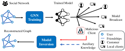
Figure 1: One motivation scenario in social networks where the attacker aims to reconstruct the friendship through the model inversion attack. Users’ friendships are sensitive relational data, and users want to keep them private. Sometimes social network data is collected with user permission to train GNN models for better service. If the attacker can obtain the trained GNN model from malicious clients, with some auxiliary knowledge crawled from the internet, model inversion attack can be performed to reconstruct the friendships among users.

However, the fact that many GNN-based applications rely on processing sensitive graph data raises great privacy concerns. Attackers may exploit the output (i.e., black-box attack) or the parameters (i.e., white-box attack) of trained graph neural networks to potentially reveal sensitive information in the training graph data. Of particular interest to this paper is the model inversion attack which aims to extract sensitive features of training data given output labels and partial knowledge of non-sensitive features. Studying model inversion attack on GNNs helps us understand the vulnerability of GNN models and enable us to evaluate and avoid privacy risks in advance.

Motivation scenario: Figure 1 shows one concrete motivation scenario of model inversion attack on GNN models. Users’ friendships are sensitive relational data, and users want to keep them private. Sometimes social network data is collected with user permission to train GNN models for better service. For example, these trained GNN models are used to classify friends or recommend advertisements. Then, the trained models are broadcast to customers or local clients. If the attacker can obtain the trained GNN model from malicious clients, with some auxiliary knowledge crawled from the internet, model inversion attack can be performed to reconstruct friendships among users.

Model inversion attack was firstly introduced by [19], where an attacker, given a linear regression model for personalized medicine and some demographic information about a patient, could predict the patient’s genetic markers. Generally, model inversion relies on the correlation between features and output labels and tries to maximize a posteriori (MAP) or likelihood estimation (MLE) to recover sensitive features. Recently, efforts have been made to extend model inversion to attack other machine learning models, in particular Convolutional Neural Networks (CNN)  [18, 3]. Thus far, most model inversion attacks are investigated in the grid-like domain (e.g., images), leaving its effect on the non-grid domain (e.g., graph-structured data) an open problem.

We draw attention to the model inversion attack that aim to extract private graph data from GNN models. We focus on the following adversarial scenario: Given the trained GNN model and some auxiliary knowledge (node labels and attributes), the adversary wants to reconstruct all the edges among nodes in the training dataset. However, directly adapting model inversion attack to graphs leads to poor attack performance due to the following reasons. Firstly, existing model inversion attack methods can barely be applied to the graph setting due to the discrete nature of graphs. Different from the continuous image data, gradient computation and optimization on binary edges of the graph are difficult. Secondly, current model inversion methods fail to exploit the intrinsic properties of graph such as sparsity and feature smoothness. In addition, existing model inversion attack methods cannot fully leverage the information of node attributes and GNN models. For example, node pairs with similar attributes or embeddings are more likely to have edges.

To address the aforementioned challenges, in our preliminary work [63], we proposed Graph Model Inversion attack (GraphMI) for edge reconstruction. GraphMI is designed with three important modules: the projected gradient module, the graph auto-encoder module, and the random sampling module. The projected gradient module is able to tackle the edge discreteness via convex relaxation while preserving graph sparsity and feature smoothness. The graph auto-encoder module is designed to take all the information of node attributes, graph topology, and target model parameters into consideration for graph reconstruction. The random sampling module is used to recover the binary adjacency matrix. With these delicately designed modules, GraphMI can effectively infer the private edges in the training graph. We systematically evaluate our attack and compare it with baseline attacks on real-world datasets from four different fields and three representative GNN methods . Based on GraphMI, we also investigate the relation between edge influence and model inversion risk and find that edges with greater influence are more likely to be reconstructed.

However, GraphMI is only performed in the white-box setting, where the attacker requires full access to the target model to take derivations with respect to the adjacency matrix [63]. Thus, it is infeasible in the more challenging hard-label black-box setting where the attacker can only query the GNN API and receive the classification results. Therefore, in this paper we extend GraphMI and propose two black-box attacks based on gradient estimation and reinforcement learning. We also explore the countermeasures against our attack including differential private training [1] and graph preprocessing based on edge perturbation. Specifically in graph preprocessing, three strategies including randomly rewiring, adding new edges and randomly flipping are tried. The key idea to is to “hide” real edges from model inversion by perturbing the graph structure. Experiments show that these defenses are not effective enough to achieve a satisfying trade-off between node classification accuracy and robustness to GraphMI.

In summary, we make the following contributions.

• We propose GraphMI, a novel model inversion attack against Graph Neural Networks. Our attack is specifically designed and optimized for extracting private graph-structured data from GNNs.

• We extend GraphMI to the black-box setting and propose two attack methods, gradient estimation and RL-GraphMI.

• We explore the countermeasures against our attack. We empirically show that our attack is still effective even with differential private training or graph preprocessing.

The rest of our paper is organized as follows: In Section 2, we review different attack and defense methods for GNNs; in Section 3, we introduce the problem formulation; in Section 4, we first introduce the design of GraphMI framework and then provide the analysis on correlation between Edge influence and inversion risk; in Section 5, we show how to extend GraphMI to the black-box setting based on gradient estimation and reinforcement learning; in Section 6, we experimentally demonstrate the attack performance of our method; in Section 7, we explore the countermeasures against GraphMI. Finally, we show the conclusion and discuss the future works in Section 8.

2 Related Work

In this section, we review research works related to our proposed attacks. We refer the readers to [62] for an in-depth overview of different GNN models, and [46, 28] for comprehensive surveys of existing adversarial attacks and defense strategies on GNNs.

2.1 Adversarial Attacks on GNNs

Existing studies have shown that GNNs are vulnerable to adversarial attacks [11, 8, 36, 50, 31, 16, 56, 65, 35, 38, 55], which deceive GNN models to make wrong predictions for graph classification or node classification. Depending on the stages when these attacks occur, these adversarial attacks can be classified into training-time poisoning attacks [34, 50, 66] and testing time adversarial attacks [9, 35, 10]. Based on the attacker’s knowledge, adversarial attacks can also be categorized into white-box attacks [56, 65] and black-box attacks [35, 38, 8].

2.2 Privacy Attacks on GNNs

Based on the attacker’s goal, privacy attacks can be categorized into several types [41], such as membership inference attack [45], model extraction attack [48], and model inversion attack [18]. Membership inference attack tries to determine whether one sample was used to train the machine learning model; Model extraction attack is one black-box privacy attack. It tries to extract information of model parameters and reconstruct one substitute model that behaves similarly to the target model. Model inversion attack, which is the focus of this paper, aims to reconstruct sensitive features corresponding to labels of target machine learning models.

Model inversion attack was firstly presented in [19] for linear regression models. M. Fredrikson et al. [18] extended model inversion attack to extract faces from shallow neural networks. They cast the model inversion as an optimization problem and solve the problem by gradient descent with modifications to the images. Furthermore, several model inversion attacks in the black-box setting or assisted with generative methods are proposed [3, 60] in the image domain. In addition, some recent papers started to study the factors affecting a model’s vulnerability to model inversion attacks theoretically [54, 57].

Different from adversarial attacks, only a few studies [51, 24, 13, 61, 26] focused on privacy attacks on GNNs. For instance, Wu et al. [51] discussed GNN model extraction attack. Given various levels of background knowledge, they tried to gather both the input-output query pairs and the graph structure to reconstruct a duplicated GNN model. He et al. [24] and Duddu et al. [13] tried to infer the edges based on node embeddings from GNNs. Zhang et al. [61] proposed three inference attacks against graph embeddings. Thus far, no researcher has explored model inversion attacks against Graph Neural Networks.

2.3 Defense of Attacks on GNNs

Most defense mechanisms focus on mitigating adversarial attacks by e.g. graph sanitization [53], adversarial training [12, 59], and certification of robustness [6]. On the other hand, to defend against privacy attacks, one of the most popular proposed countermeasures is differential privacy (DP) [14]. Differential privacy is a notion of privacy that entails that the outputs of the model on neighboring inputs are close. This privacy requirement ends up obscuring the impact of any individual training instance on the model output. Abadi et al. [1] proposed DP-SGD, which ensures $(\epsilon,\delta)-$DP through adding Gaussian noise to clipped gradients in training iterations. Hay et al. [23] firstly extend differential privacy to the graph setting. Since then, extensive efforts have been made on computing graph statistics under edge or node differential privacy such as degree distribution [23], cut queries [4], and sub-graph counting queries [5]. These methods are useful for analyzing graph statistics but insufficient for training a GNN model with DP. To evaluate the effectiveness of GraphMI, we adapt DP-SGD and propose three graph preprocessing methods as countermeasures.

3 Problem Formulation

We begin by providing preliminaries on GNNs. Then we will present the problem definition of model inversion attack on graph neural networks.

3.1 Preliminaries on GNNs

Before defining GNN, we firstly introduce the following notations of graph. Let $G=(\mathcal{V,E})$ be an undirected and unweighted graph, where $\mathcal{V}$ is the vertex (i.e. node) set with size $|\mathcal{V}|=N$, and $\mathcal{E}$ is the edge set. Denote $A\in\{0,1\}^{|\mathcal{V}|\times|\mathcal{V}|}$ as an adjacent matrix containing information of network topology and $X\in\mathbb{R}^{|\mathcal{V}|\times l}$ as a feature matrix with dimension $l$. A graph can also be expressed as $G=\{A,X\}$. One task that GNN models are commonly used for is semi-supervised node classification [30]. In a GNN model for node classification, each node $i$ is associated with a feature vector $\textbf{x}_{i}\in\mathbb{R}^{l}$ and a scalar label $y_{i}$. Given the adjacency matrix $A$ and the labeled node data $\{(\textbf{x}_{i},y_{i})\}_{i\in\mathcal{T}}$ ($\mathcal{T}$ denotes the training set), GNN is trained to predict the classes of unlabeled nodes.

Formally, the $k$-th layer of a GNN model obeys the message passing rule and can be modeled by one message passing phase and one aggregation update phase:

$$m_{v}^{k+1}=\mathop{\sum}_{u\in\mathcal{N}(v)}\mathbf{M}_{k}(h_{v}^{k},h_{u}^{k},e_{uv}),$$ (1)

$$h_{v}^{k+1}=\mathbf{U}_{k}(h_{v}^{k},m_{v}^{k+1}),$$ (2)

where $\mathbf{M}_{k}$ denotes the message passing function and $\mathbf{U}_{k}$ is the vertex update function. $\mathcal{N}(v)$ is the neighbors of $v$ in graph $G$. $h_{v}^{k}$ is the feature vector of node $v$ at layer $k$ and $e_{uv}$ denotes the edge feature. $h^{0}_{v}=\textbf{x}_{v}$ is the input feature vector of node $v$.

Specifically, Graph Convolutional Network (GCN) [30], a well-established method for semi-supervised node classification, obeys the following rule to aggregate neighboring features:

$$H^{k+1}=\sigma\big{(}\hat{D}^{-\frac{1}{2}}\hat{A}\hat{D}^{-\frac{1}{2}}H^{k}W^{k}\big{)},$$ (3)

where $\hat{A}=A+I_{N}$ is the adjacency matrix of the graph $G$ with self connections added and $\hat{D}$ is a diagonal matrix with $\hat{D}_{ii}=\sum_{j}\hat{A}_{ij}$. $\sigma(\cdot)$ is the ReLU function. $H^{k}$ and $W^{k}$ are the feature matrix and the trainable weight matrix of the $k$-th layer respectively. $H^{0}=X$ is the input feature matrix. Note that in most of this paper, we focus on two-layer GCN for the node classification. Later, we show that our graph model inversion attack can extend to other types of GNNs, including GAT [49] and GraphSAGE [22].

3.2 Problem Definition

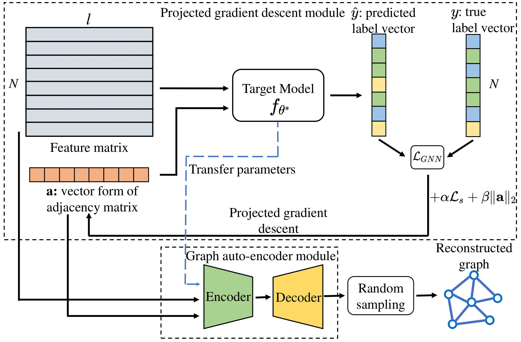
Figure 2: Illustration of the proposed GraphMI. Generally, GraphMI consists of three modules: projected gradient descent module, graph auto-encoder module and random sampling module. Firstly, the projected gradient descent module gets the initial reconstructed adjacency matrix through projected gradient descent. Then, the graph auto-encoder module post-process the reconstructed adjacency matrix. Finally, we can sample a discrete adjacency matrix from the edge probability matrix.

We refer to the trained model subjected to model inversion attack as the target model. In this paper, we will firstly train a GNN for node classification task from scratch as the target model. We assume a threat model similar to the existing model inversion attacks [18].

3.2.1 Attacker’s Knowledge and Capability

In this paper, we investigate model inversion attacks against GNN in both white-box and hard-label black-box settings. In the white-box setting, the attacker is assumed to have full access to the target model $f_{\theta}$ including the model architecture and all the parameters $\theta$. In addition to the target model $f_{\theta}$, the attacker may have other auxiliary knowledge to facilitate model inversion such as node labels, node attributes, node IDs or edge density. We will discuss the impact of auxiliary knowledge and the number of node labels on attack performance in the following sections. In the hard-label black-box setting, the attacker is only allowed to query the target GNN model $f_{\theta}$ with an input graph and obtain the predicted labels.

3.2.2 Objective of Attack

Assuming the target GNN model $f_{\theta}$ is first trained on $G=\{A,X\}$, the objective of attacker $\mathcal{A}$ is:

$$\textup{max }s(\widetilde{A},A),s.t.~{}\widetilde{A}=\mathcal{A}(X,Y,f_{\theta}),$$ (4)

where $Y$ is the vector of node labels and $s(\cdot,\cdot)$ is the similarity function to measure the similarity of adjacency matrices e.g. Weisfeiler-Lehman kernel [44]. $\widetilde{A}$ is the reconstructed adjacency matrix by the attacker $\mathcal{A}$.

Algorithm 1 GraphMI

Input: Target GNN model $f_{\theta}$; Node label vector $Y$; Node feature matrix $X$; Learning rate, $\eta_{t}$; Iterations $T$;
Output: Reconstructed $A$

1:  $\mathbf{a}^{(0)}$ is set to zeros

2:  Let $t=0$

3:  while t <T do

4:     Gradient descent: $\mathbf{a}^{(t)}=\mathbf{a}^{(t-1)}-\eta_{t}\nabla\mathcal{L}_{attack}(\mathbf{a})$;

5:     Call Projection operation in (14)

6:  end while

7:  Call Graph auto-encoder module in (15)

8:  Call Random sampling module in Algorithm 2.

9:  return $A$

4 White-Box Attack: GraphMI

Next we introduce GraphMI, our proposed white-box model inversion attack against GNN models. The target model $f_{\theta}$ is firstly trained to minimize the loss function $\mathcal{L}(X,Y,A,\theta)$:

$$\theta^{*}={\textup{arg }}\mathop{\textup{min}}\limits_{\theta}\mathcal{L}(X,Y,A,\theta).$$ (5)

Without ambiguity, we still use $\theta$ as the trained model parameters in the rest of this paper. Then, given the trained model and its parameters, GraphMI aims to find the adjacency matrix $\widetilde{A}$ that maximizes the posterior possibility:

$$\widetilde{A}={\textup{arg }}\mathop{\textup{max}}\limits_{A}P(A|X,Y,f_{\theta}).$$ (6)

4.1 Attack Overview

Figure 2 shows the overview of GraphMI. Generally, GraphMI is one optimization-based attack method, which firstly employs projected gradient descent on the graph to find the “optimal” network topology for node labels. Then the adjacency matrix and feature matrix will be sent to the graph auto-encoder module of which parameters are transferred from the target model. Finally, we can interpret the optimized graph as the edge probability matrix and sample a binary adjacency matrix. We summarize GraphMI in Algorithm 1.

4.2 Details of Modules

4.2.1 Projected Gradient Descent Module

We treat model inversion on GNNs as one optimization problem: given node features or node IDs, we want to minimize the cross-entropy loss between true labels $y_{i}$ and predicted labels $\hat{y_{i}}$ from the target GNN model $f_{\theta}$. The intuition is that the reconstructed adjacency matrix will be similar to the original adjacency matrix if the cross-entropy loss between true labels and predicted labels is minimized. The attack loss on node $i$ is denoted by $\ell_{i}(A,f_{\theta},\textbf{x}_{i},y_{i})$ where $A$ denotes the reconstructed adjacency matrix for brevity, $\theta$ is the model parameter of the target model $f$ and $\textbf{x}_{i}$ denotes the node feature vector of node $i$. The attack objective function can be formulated as:

$$\begin{split}\mathop{\textup{min}}\limits_{A\in\{0,1\}^{N\times N}}\mathcal{L}_{GNN}(A)&=\frac{1}{N}\sum_{i=1}^{N}\ell_{i}(A,f_{\theta},\textbf{x}_{i},{y_{i}})\\ s.t.\quad A&=A^{\top}.\end{split}$$ (7)

In many real-world graphs, such as social networks, citation networks, and web pages, connected nodes are likely to have similar features [53]. Based on this observation, we need to ensure the feature smoothness in the optimized graph. The feature smoothness can be captured by the following loss term $\mathcal{L}_{s}$:

$$\mathcal{L}_{s}=\frac{1}{2}\sum_{i,j=1}^{N}A_{i,j}(\textbf{x}_{i}-\textbf{x}_{j})^{2},$$ (8)

where $A_{i,j}$ indicates the connection between node $v_{i}$ and $v_{j}$ in the optimized graph and $(\textbf{x}_{i}-\textbf{x}_{j})^{2}$ measures the feature difference between $v_{i}$ and $v_{j}$. $\mathcal{L}_{s}$ can also be represented as:

$$\mathcal{L}_{s}=tr(X^{\top}LX),$$ (9)

where $L=D-A$ is the laplacian matrix of $A$ and $D$ is the diagonal matrix of $A$. In this paper, to make feature smoothness independent of node degrees, we use the normalized lapacian matrix $\hat{L}=D^{-1/2}LD^{-1/2}$ instead:

$$\mathcal{L}_{s}=tr(X^{\top}\hat{L}X)=\frac{1}{2}\sum_{i,j=1}^{N}A_{i,j}(\frac{\textbf{x}_{i}}{\sqrt{d_{i}}}-\frac{\textbf{x}_{j}}{\sqrt{d_{j}}})^{2},$$ (10)

where $d_{i}$ and $d_{j}$ denote the degree of node $v_{i}$ and $v_{j}$. The authors also notice that recent studies [27, 32] show that some heterophily graphs do not have the characteristic of feature smoothness. We left dealing with this class of graph for the future work. To encourage the sparsity of graph structure, $F$ norm of adjacency matrix $A$ is also added to the loss function as one regularization term. The final objective function is:

$$\begin{split}{\textup{arg }}\mathop{\textup{min}}\limits_{A\in\{0,1\}^{N\times N}}\mathcal{L}_{attack}&=\mathcal{L}_{GNN}+\alpha\mathcal{L}_{s}+\beta\|A\|_{F}\\ s.t.\quad A&=A^{\top},\end{split}$$ (11)

where $\alpha$ and $\beta$ are hyper-parameters that control the weight of feature smoothing and graph sparsity. Solving equation (11) is a combinatorial optimization problem due to edge discreteness. For ease of gradient computation and update, we firstly replace the symmetric reconstructed adjacency matrix $A$ with its vector form $\mathbf{a}$ that consists of $n\coloneqq N(N-1)/2$ unique variables in $A$. Adjacency matrix $A$ and vector $\mathbf{a}$ can be converted to each other easily, which ensures the optimized adjacency matrix is symmetric. Then we relax $\mathbf{a}\in\{0,1\}^{n}$ into convex space $\mathbf{a}\in[0,1]^{n}$. We can perform model inversion attack by firstly solving the following optimization problem:

$${\textup{arg }}\mathop{\textup{min}}\limits_{\mathbf{a}\in[0,1]^{n}}\mathcal{L}_{attack}=\mathcal{L}_{GNN}+\alpha\mathcal{L}_{s}+\beta\|\mathbf{a}\|_{2}.$$ (12)

The continuous optimization problem (12) is solved by projected gradient descent (PGD):

$$\mathbf{a}^{t+1}=P_{[0,1]}\big{[}\mathbf{a}^{t}-\eta_{t}g_{t}\big{]},$$ (13)

where $t$ is the iteration index of PGD, $\eta_{t}$ is the learning rate, $g_{t}$ is the gradients of loss $\mathcal{L}_{attack}$ in 11 evaluated at $\textbf{a}^{t}$, and

$$P_{[0,1]}[x]=\left\{\begin{array}[]{rcl}0&&x<0\\ 1&&x>1\\ x&&otherwise.\end{array}\right.$$ (14)

is the projection operator.

4.2.2 Graph Auto-encoder Module

In GraphMI, we propose to use graph auto-encoder (GAE) [29] to post-process the optimized adjacency matrix $A$. GAE is composed of two components: encoder and decoder. We transfer part of the parameters from the target model $f_{\theta}$ to the encoder. Specifically, feature matrix and adjacency vector $\mathbf{a}$ are sent to the $f_{\theta}$ and the node embedding matrix $Z$ is generated by taking the penultimate layer of the target model $f_{\theta}$, which is denoted as $H_{\theta}(\mathbf{a},X)$. Then the decoder will reconstruct adjacency matrix $A$ by applying logistic sigmoid function to the inner product of $Z$:

$$A={\rm sigmoid}(ZZ^{\top}),{\rm with}~{}Z=H_{\theta}(\mathbf{a},X).$$ (15)

The node embeddings generated by the graph auto-encoder module encode the information from node attributes, graph topology, and the target GNN model. Intuitively, node pairs with close embeddings are more likely to form edges. In experiments, we conduct ablation studies to show the impact of the graph auto-encoder module on the attack performance.

4.2.3 Random Sampling Module

After the optimization problem is solved, the solution $A$ can be interpreted as a probabilistic matrix, which represents the possibility of each edge. We could use random sampling to recover the binary adjacency matrix. Firstly, we need to calculate the number of sampling edges $\lfloor\rho n\rfloor$ given the estimated graph density $\rho$. The estimated graph density $\rho$ can be obtained from public graphs from the same domain. In the experiments, we will show how the discrepancy between the estimated density and the ground truth density affects the attack performance. Generally, GraphMI is robust to the graph density estimation. Then we take $K$ trials to sample edges based on the probabilistic matrix. Finally, we choose the adjacency matrix with the smallest attack loss $\mathcal{L}_{attack}$. More details are shown in Algorithm 2.

Algorithm 2 Random sampling from probabilistic vector to binary adjacency matrix

Input: Probabilistic vector $\mathbf{a}$, number of trials $K$
Parameter: Edge density $\rho$
Output: Binary matrix $A$;

1:  Normalize probabilistic vector: $\hat{\mathbf{a}}$ = $\mathbf{a}/\|\mathbf{a}\|_{1}$

2:  for k = 1,2 $\cdots$ K do

2:     Draw binary vector $\mathbf{a}^{(k)}$ by sampling $\lfloor\rho n\rfloor$ edges according to probabilistic vector $\hat{\mathbf{a}}$.

3:  end for

4:  Choose a vector $\mathbf{a}^{*}$ from $\{\mathbf{a}^{(k)}\}$ which yields the smallest loss $\mathcal{L}_{attack}$.

5:  Convert $\mathbf{a}^{*}$ to binary adjacency matrix $A$

6:  return $A$

4.3 Analysis on Correlation between Edge Influence and Inversion Risk

In previous work [54], researchers found feature influence to be an essential factor in incurring privacy risk. In our context of graph model inversion attack, sensitive features are edges. Here we want to characterize the correlation between edge influence and inversion risk. Given label vector $Y$, adjacency matrix $A$ and feature matrix $X$, the performance of target model $f_{\theta}$ for the prediction can be measured by prediction accuracy:

$$ACC(f_{\theta},A,X)=\frac{1}{N}\sum_{i=1}^{N}\mathbf{1}[f_{\theta}^{i}(A,X)=y_{i}],$$ (16)

where, $f_{\theta}^{i}(A,X)$ is the predicted label for node $i$. The influence of edge $e$ can be defined as:

$${\mathcal{I}}(e)=ACC(f_{\theta},A,X)-ACC(f_{\theta},A_{-e},X),$$ (17)

where $A_{-e}$ denotes removing the edge $e$ from the adjacency matrix $A$. [54] proposed to use adversary advantage to characterize model inversion risk of features. The model inversion advantage $Adv$ of adversary $\mathcal{A}$ is defined to be $P[\mathcal{A}(X,f_{\theta})=e]-1/2$, where $P[\mathcal{A}(X,f_{\theta})=e]$ is the probability that adversary $\mathcal{A}$ correctly infer the existence of edge $e$. Next, we introduce our theorem.

Theorem 1

$Adv(e_{i})\leq Adv(e_{j}),~{}\forall e_{i},e_{j}\in\mathcal{E}\cap\mathcal{I}(e_{i})\leq\mathcal{I}(e_{j})$ i.e. The adversary advantage is greater for edges with greater influence.

Proof 1

Our detailed proof in shown in Appendix A.

Intuitively, edges with greater influence are more likely to be recovered by GraphMI because these edges have a greater correlation with the model output. In the following section, we will validate our theorem with experiments.

5 Black-box Attack

We illustrate the white-box attack GraphMI in the above section. In this section, we consider the strictest hard-label black-box setting. Specifically, the attacker is only allowed to query the target GNN model $f_{\theta}$ with an input graph and obtain only the predicted hard label (instead of a confidence vector that indicates the probabilities that the graph belongs to each class) for the input graph. All the other knowledge, e.g., training graphs, structures, and parameters of the target GNN model are unavailable to the attacker. Such a black-box situation brings more challenges to the design of model inversion attacks because the attacker is unable to take the derivative of the adjacency matrix directly. In this section, we propose two methods based on gradient estimation and reinforcement learning.

5.1 Gradient Estimation

We first introduce the projected gradient estimation algorithm to solve the problem of black-box attack. With zeroth order oracle, we can estimate the gradient of $\mathcal{L}_{attack}$ in Equ.12 via computing $(\mathcal{L}_{attack}(a+\mu u)-\mathcal{L}_{attack}(a-\mu u))/2\mu$, where $u$ denotes a normalized direction vector sampled randomly from a uniform distribution over a unit sphere [33, 43, 20], and $\mu$ is a step constant. Note that since the attacker is only accessible to the predicted hard labels, $\mathcal{L}_{GNN}$ in $\mathcal{L}_{attack}$ cannot be computed in the black-box setting. We use the error rate $\frac{1}{N}\sum_{i=1}^{N}\mathbf{1}(f_{\theta}^{i}(A,X)\neq y_{i})$ instead. To ease the noise of gradients, we average the gradients in different directions to estimate the derivative of $\mathcal{L}_{attack}$ as follows:

$$\hat{\nabla}\mathcal{L}_{attack}(a)=\frac{d}{q}\sum_{j=1}^{q}\frac{\mathcal{L}_{attack}(a+\mu u_{j})-\mathcal{L}_{attack}(a-\mu u_{j})}{2\mu}u_{j},$$ (18)

where $q$ is the number of queries to estimate the gradient $\hat{\nabla}\mathcal{L}_{attack}$ and $d$ is the dimension of optimization variables. After computing the estimated gradient, the attacker update the vector of adjacency matrix by projected gradient descent in Equ.13. The following theorem shows the convergence guarantees of our zeroth-order projected gradient descent for the black-box attack.

Assumption 1

The loss function $\mathcal{L}_{attack}$ is $L_{1}$-Lipschitz continuous for a finite positive constant $L_{1}$.

Assumption 2

The loss function $\mathcal{L}_{attack}$ is differentiable and has $L_{2}$-Lipschitz continuous gradients for a finite positive constant $L_{2}$.

Theorem 2

Suppose Assumption 1$\&$2 hold. If we randomly pick $a_{r}$, whose dimension is $d$, from $\{a_{t}\}_{t=0}^{T-1}$ with probability $P(r=t)=\frac{2\eta_{t}-L_{2}\eta_{t}^{2}}{\sum_{t=0}^{T-1}2\eta_{t}-L_{2}\eta_{t}^{2}}$ Then, we have the following bound on the convergence rate with $\eta_{t}=\mathcal{O}(\frac{1}{\sqrt{T}})$ and $\mu=\mathcal{O}(\frac{1}{\sqrt{dq}})$:

$$\mathbb{E}[\|P_{[0,1]}(a_{r},\hat{\nabla}\mathcal{L}_{attack}(a_{r}),\eta_{r})\|^{2}]=\mathcal{O}(\frac{1}{\sqrt{T}}+\frac{d+q}{q}),$$ (19)

where $P_{[0,1]}(a_{r},\hat{\nabla}\mathcal{L}_{attack}(a_{r}),\eta_{r})\coloneqq(1/\eta_{r})[a_{r}-P_{[0,1]}(a_{r}-\eta_{r}\hat{\nabla}\mathcal{L}_{attack}(a_{r}))$ is the rectified gradient.

Proof 2

We defer the proof to the Appendix B.

5.2 RL-GraphMI

Deep reinforcement learning (DRL) offers a promising approach for realizing black-box graph model inversion attacks. Firstly, the addition of edges between nodes can be naturally modeled by actions in a reinforcement learning model. Secondly, the non-linear mapping between the graph structure and its low-dimensional representation can be well captured by a deep neural network.

The key idea behind RL-GraphMI is to use a deep reinforcement learning agent to iteratively perform actions aimed at reconstructing the edges of the training graph. Formally, We model the reconstruction of edges by a Finite Horizon Markov Decision Process $(S,A,P,R,\gamma)$ where $S$ denotes the set of states, $A$ the set of actions, $P$ the matrix of state transition probabilities, $R$ is the reward function, and $\gamma<1$ is a discounting factor that discounts delayed reward relative to immediate reward.

5.2.1 States and Actions

The state $s_{t}$ contains the intermediate reconstructed graph $G_{t}$ and the node labels ${y_{i}}$. We use a two layer graph convolutional network and a two layer neural network to encode $G_{t}$ and ${y_{i}}$ respectively. The embedding of the node $e(v)$ is obtained by concatenating the structure embedding from $G_{t}$ and label embedding from $y_{i}$. The embedding of $s_{t}$ is obtained by averaging all the node embeddings.

A single action at time step $t$ is $a_{t}\in V\times V$. However, simply performing actions in space $\mathcal{O}(|V|^{2})$ is too expensive. Following [11] and [47], we adopt a hierarchical decomposition of actions to reduce the action space. At time $t$, the DRL agent first performs an action $a_{t}^{(1)}$ to select the first node and then pick the second node using $a_{t}^{(2)}$. After $a_{t}^{(1)}$ and $a_{t}^{(2)}$, a new edge is added between the selected two nodes if there was no edge. With the hierarchy action $a_{t}=(a_{t}^{(1)},a_{t}^{(2)})$, the trajectory of the proposed MDP is $(s_{0},a_{0}^{(1)},a_{0}^{(2)},r_{0},s_{1},\cdots,s_{T-1},a_{T-1}^{(1)},a_{T-1}^{(2)},s_{T},r_{T})$.

5.2.2 Policy Network

After [11] and [47], we use Q-learning to find a policy that is optimal in the sense that it maximizes the expected value of the total reward over any and all successive steps, starting from the current state. Q-learning is an off-policy optimization which aims to satisfy the the Bellman optimality equation as follows:

$$Q^{*}(s_{t},a_{t})=r(s_{t},a_{t})+\gamma\mathop{\textup{max}}\limits_{a_{t}^{\prime}}Q^{*}(s_{t+1},a^{\prime}_{t}).$$ (20)

The greedy policy to select the action $a_{t}$ with respect to $Q^{*}$:

$$a_{t}=\pi(s_{t})=\mathop{\textup{arg max}}\limits_{a_{t}}Q^{*}(s_{t},a_{t}).$$ (21)

In experiments, We adopt a hierarchical Q function $Q=\{Q^{(1)},Q^{(2)}\}$ for modeling the two actions:

$$Q^{(1)}(s_{t},a_{t}^{(1)};\phi^{(1)})=W_{1}^{(1)}\sigma(W_{2}^{(1)}[e(v_{a_{t}^{(1)}})\|e(s_{t})]),$$ (22)

where $\phi^{(1)}=\{W_{1}^{(1)},W_{2}^{(1)}\}$ denotes the trainable weights and $\|$ is the concatenation operation. $e(s_{t})$ is the state embedding and $e(v_{a_{t}^{(1)}})$ is the node embedding of first selected node. With the first action $a_{t}^{(1)}$ selected, the DRL agent picks the second action $a_{t}^{(2)}$ based on $Q^{(2)}$ as follows:

$$Q^{(2)}(s_{t},a_{t}^{(1)},a_{t}^{(2)};\phi^{(2)})=W_{1}^{(2)}\sigma(W_{2}^{(2)}[e(v_{a_{t}^{(2)}})\|e(v_{a_{t}^{(1)}})\|e(s_{t})]),$$ (23)

where $\phi^{(2)}=\{W_{1}^{(2)},W_{2}^{(2)}\}$ denotes the trainable weights. The action value function $Q^{(2)}$ scores the candidate nodes for establishing an edge based on the state $s_{t}$, and $a_{t}^{(1)}$.

5.2.3 Reward Function

We design the reward function $r(s_{t},a_{t}^{(1)},a_{t}^{(2)})$ based on accuracy $ACC_{t}=\frac{1}{N}\sum_{i=1}^{N}\mathbf{1}[f_{\theta}^{i}(A_{t},X)=y_{i})]$ where $A_{t}$ is the adjacency matrix of $G_{t}$. However, direct use of $ACC_{t}$ as the reward could slow down training since the accuracy might not differ significantly between two consecutive states. Hence, we design a guiding binary reward $r_{t}$ to be 1 if the action $a_{t}=(a_{t}^{(1)},a_{t}^{(2)})$ can increase the accuracy at time t, and to be -1 otherwise:

$$r(s_{t},a_{t}^{(1)},a_{t}^{(2)})=\left\{\begin{array}[]{rcl}1&&ACC_{t}\geq ACC_{t-1}\\ -1&&otherwise.\end{array}\right.$$ (24)

5.2.4 Terminal

In RL-GraphMI, the DRL agent stops to take further actions once the number of edges reaches the predefined number which can be estimated by the graph density.

Algorithm 3 The training algorithm of RL-GraphMI

Input:Target GNN model $f_{\theta}$; Node label vector $Y$; Node feature matrix $X$; Learning rate, $\eta_{t}$; Training Iterations $T$; Maximum Edges $\Delta$; Update Period $C$
Output:Reconstructed A

1:  Initialize action-value function Q with random parameters $\phi$

2:  Set target function $\hat{Q}$ with parameters $\phi^{-}=\phi$

3:  Initialize replay memory buffer $\mathcal{M}$

4:  while episode <T do

5:     Initialize edge set of the adjacency matrix $A$

6:     while t <$\Delta$ do

7:        Compute state representation

8:        With probability $\epsilon$ select a random action $a_{t}^{(1)}$, otherwise select $a_{t}^{(1)}$ based on Eq.(22)

9:        With probability $\epsilon$ select a random action $a_{t}^{(2)}$, otherwise select $a_{t}^{(2)}$ based on Eq.(23)

10:        Compute $r_{t}$ according to Eq.(24)

11:        Set $s_{t+1}=\{s_{t},a_{t}^{(1)},a_{t}^{(2)}\}$

12:        $E_{A}\leftarrow E_{A}\cup(a_{t}^{(1)},a_{t}^{(2)})$

13:        Store $\{s_{t},a_{t}^{(1)},a_{t}^{(2)},r_{t},s_{t+1}\}$ in memory $\mathcal{M}$

14:        Sample minibatch transition randomly from $\mathcal{M}$

15:        Update parameter according to Eq.(25)

16:        Every C steps $\phi^{-}=\phi$;

17:     end while

18:  end while

19:  return $A$

5.2.5 Training Algorithm

To train the RL-GraphMI, we adopt the experience replay technique with memory buffer $\mathcal{M}$ [37]. The trainable parameters in RL-GraphI is denoted as $\phi$. The key idea behind experience replay is to randomizes the order of data used by Q learning, so as to remove the correlations in the observation sequence. We simulate action selection and store the resulting data in a memory buffer $\mathcal{M}$. During training, a batch of experience $(s,a,s^{\prime})$ where $a=\{a^{(1)},a^{(2)}\}$ is drawn uniformly from the stored memory buffer $\mathcal{M}$. The Q-learning loss function is similar to [37] as:

$$\mathbb{E}_{(s,a,s^{\prime})\sim\mathcal{M}}[(r+\gamma\max_{a^{\prime}}\hat{Q}(s^{\prime},a^{\prime}|\phi^{-})-Q(s,a|\phi))^{2}],$$ (25)

where $\hat{Q}$ represents the target action-value function and its parameters $\phi^{-}$ are updated with $\phi$ every C steps. To improve the stability of the algorithm, we clip the error term between $-1$ and $+1$. The agent adopts $\epsilon$-greedy policy that select a random action with probability $\epsilon$. The overall training framework is summarized in Algorithm 3.

5.3 Computational Complexity

In GraphMI, we take derivatives with respect to the adjacency matrix $A$. The computational complexity of GraphMI is $N^{2}T$ where $N$ is the number of nodes, and $T$ is the total iterations. The computational overhead of gradient estimation and RL-GraphMI are $N^{2}qT$ and $N^{2}\Delta T$ respectively, where $q$ is the number of queries and $\Delta$ is the number of maximum edges.

TABLE I: Dataset statistics

Datasets	Nodes	Edges	Classes	Features
Cora	2,708	5,429	7	1,433
Citeseer	3,327	4,732	6	3,703
Polblogs	1,490	19,025	2	-
USA	1,190	13,599	4	-
Brazil	131	1,038	4	-
AIDS	31,385	64,780	38	4
ENZYMES	19,580	74,564	3	18

6 Attack Results

TABLE II: Results of model inversion attack on GCN ($\%$). We repeat 5 times and report the means and standard deviations. The best result for each dataset are bolded

Method	Cora		Citeseer		Polblogs		USA		Brazil		AIDS
	AUC	AP	AUC	AP	AUC	AP	AUC	AP	AUC	AP	AUC	AP
Attr. Sim.	80.3$\pm$1.3	80.8$\pm$1.6	88.9$\pm$1.7	89.1$\pm$1.8	-	-	-	-	-	-	73.1$\pm$1.8	72.7$\pm$2.0
Emb. Sim.	81.6$\pm$1.1	82.2$\pm$1.4	87.2$\pm$1.5	86.1$\pm$1.4	66.9$\pm$1.6	67.4$\pm$1.6	64.8$\pm$0.8	65.1$\pm$0.7	67.2$\pm$1.4	70.1$\pm$1.2	74.0$\pm$1.3	72.9$\pm$1.2
MAP	74.7$\pm$1.6	71.8$\pm$1.5	69.3$\pm$0.8	75.5$\pm$0.9	68.8$\pm$1.1	75.1$\pm$1.3	59.4$\pm$1.5	61.1$\pm$1.7	63.8$\pm$1.2	66.1$\pm$1.3	64.2$\pm$1.3	65.3$\pm$1.4
GraphMI	86.8$\pm$1.3	88.3$\pm$1.2	87.8$\pm$0.6	88.5$\pm$0.5	79.3$\pm$0.6	79.7$\pm$0.8	80.6$\pm$1.4	81.3$\pm$1.6	86.6$\pm$1.0	88.8$\pm$0.9	80.2$\pm$1.0	80.9$\pm$1.5

In this section, we present the experimental results to show the effectiveness of GraphMI in both white-box and hard-label black-box settings.

6.1 Experimental Settings

Datasets: Our graph model inversion attack method is evaluated on 7 public datasets from 4 categories. The detailed statistics of them are listed in Table I.

• Citation Networks: We use Cora and Citeseer [42]. Here, nodes are documents with corresponding bag-of-words features and edges denote citations among nodes. Class labels denote the subfield of research that the papers belong to.

• Social Networks: Polblogs [2] is the network of political blogs whose nodes do not have features.

• Air-Traffic Networks: The air-traffic networks are based on flight records from USA and Brazil. Each node is an airport and an edge indicates a commercial airline route between airports. Labels denote the level of activity in terms of people and flights passing through an airport [39].

• Chemical Networks: AIDS [40] and Enzymes [7] are chemical datasets that contain many molecure graphs, each node is an atom and each link represents chemical bonds.

6.1.1 Target Models:

In our evaluation, we use 3 state-of-the-art GNN models: GCN [30], GAT [49] and GraphSAGE [22]. The parameters of the models are the same as those set in the original papers. To train a target model, 10% randomly sampled nodes are used as the training set. All GNN models are trained for 200 epochs with an early stopping strategy based on convergence behavior and accuracy on a validation set containing 20% randomly sampled nodes. In GraphMI attack experiments, attackers have labels of all the nodes and feature vectors. All the experiments are conducted on 1 Tesla V100 GPU.

6.1.2 Parameter Settings:

In experiments, we set $\alpha=0.001$, $\beta=0.0001$, $\eta_{t}=0.1$, $K=20$ and $T=100$ as the default setting. We show how to find optimal values for hyper-parameters in the following section. For other parameters in gradient estimation and RL-GraphMI, we set $q=100$, $\mu=0.01$, $\Delta=\lfloor n\rho_{g}\rfloor$, and $C=10$ as default ($\rho_{g}$ is the ground truth graph density). In each experiment, we repeat the attack for 5 times and report the average attack performance with standard deviations to ease the influence of randomness.

6.1.3 Metrics:

Since our attack is unsupervised, the attacker cannot find a threshold to make a concrete prediction through the algorithm. To evaluate our attack, we use AUC (area under the ROC curve) and AP (average precision) as our metrics, which is consistent with previous works [29]. In experiments, we use all the edges from the training graph and the same number of randomly sampled pairs of unconnected nodes (non-edges) to evaluate AUC and AP. The higher AUC and AP values imply better attack performance. An AUC or AP value of 1 implies maximum performance (true-positive rate of 1 with a false-positive rate of 0) while an AUC or AP value of 0.5 means performance equivalent to random guessing.

For the black-box attack, two another metrics are considered for evaluation: 1) Average Queries (AQ), i.e., the average number of queries used in the whole attack. 2) Average Time (AT), i.e., the average time used in the whole attack. An attack has better attack performance if it has a smaller AQ and AT.

6.1.4 Baselines:

There are three baseline methods, Attribute Similarity (abbreviated as Attr. Sim.), Embedding Similarity (abbreviated as Emb. Sim.), and MAP.

• Attribute Similarity is measured by cosine distance among node attributes, which is commonly used in previous works [25]. A higher similarity typically indicates a higher probability of edge existence between two nodes.

• Embedding Similarity calculates the cosine distance among the embedding of nodes, which is similar to the Attribute Similarity. The node embeddings can be obtained by taking the node representations from the penultimate layer of the target graph neural network.

• The model inversion method from [18] MAP is adapted to the graph setting as another baseline.

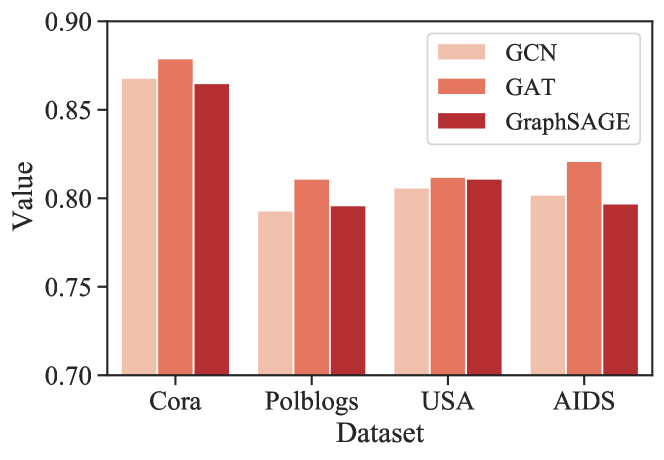
Figure 3: Attack performance of GraphMI on different Graph Neural Networks. GraphMI is agnostic to the architecture of graph neural networks and achieves success on GCN, GAT, and GraphSAGE.

6.2 Results and Discussions

TABLE III: Compare the reconstructed graph and the original graph with respect to graph isomorphism and macro-level graph statistics ($\%$). We repeat 5 times and report the means and standard deviations.

Datasets	Iso.	Degree	LCC Dist.	BC Dist.	CC Dist.
Cora	93.7$\pm$1.3	93.2$\pm$0.4	99.9$\pm$0.1	99.9$\pm$0.1	99.9$\pm$0.1
Citeseer	94.6$\pm$1.6	96.2$\pm$0.8	99.9$\pm$0.1	99.9$\pm$0.1	99.7$\pm$0.2
Polblogs	84.8$\pm$1.5	81.6$\pm$2.6	99.4$\pm$0.2	99.9$\pm$0.1	75.8$\pm$4.2
USA	86.5$\pm$0.9	88.5$\pm$1.0	99.5$\pm$0.1	99.8$\pm$0.2	86.5$\pm$1.2
Brazil	86.9$\pm$1.1	91.2$\pm$1.3	99.7$\pm$0.1	99.8$\pm$0.1	77.6$\pm$4.5
AIDS	87.8$\pm$1.4	84.7$\pm$1.9	99.2$\pm$0.3	99.6$\pm$0.1	80.2$\pm$3.7
Enzymes	82.3$\pm$1.5	75.5$\pm$3.4	98.8$\pm$0.2	98.1$\pm$0.1	78.7$\pm$2.9

6.2.1 Attack Performance

Results for model inversion attacks on GCN are summarized in table II. Note that some datasets such as Polblogs dataset do not have node attributes so we assign one-hot vectors as their attributes. They are not applicable for the attack based on attribute similarity. As can be observed in table II, GraphMI achieves the best performance across nearly all the datasets, which demonstrates the effectiveness of GraphMI. For instance, GraphMI achieves an average attack AUC of 86.8$\%$ and an average attack AP of 88.3$\%$ on the Cora dataset, which exceeds the best baseline method by at least 5 percent points. One exception is Citesser where the attack performance of GraphMI is relatively lower than attribute similarity, which could be explained by more abundant node attribute information of Citeseer compared with other datasets. Thus using node attribute similarity alone could achieve good performance on the Citesser dataset.

In figure 3, we show the attack performance of GraphMI on three GNNs. In general, GraphMI can achieve success on all three GNNs. Specially, we observe that GraphMI has better attack performance on the GAT model. This may be explained by the fact that GAT model is more powerful at node classification [49]. Thus, it is able to build a stronger correlation between graph topology and node labels. GraphMI can take advantage of such a stronger correlation and achieve better attack performance.

In figure 4(a), we present the influence of node label proportion on attack performance. As can be observed from the plot, with more node labels, the attack performance will increase gradually. This is because more node labels offer more information and regularization (Equ. 7), which the attacker can exploit to infer the training graph. Moreover, GraphMI is robust to the number of node labels. For example, GraphMI can still achieve over 80 $\%$ AUC and AP when only 20$\%$ node labels are available.

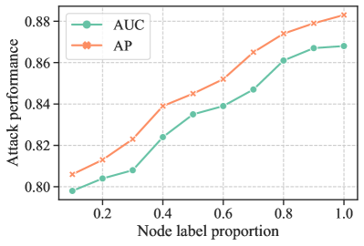
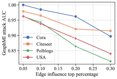
Figure 4: Impact of node label proportion (a) and edge influence (b) on the Cora dataset.

6.2.2 Graph Isomorphism and Macro-level Graph Statistics

The aforementioned results show that GraphMI can reconstruct the training graph well at the edge level by measuring AUC or AP. Further, we are interested in how the reconstructed graph resembles the training graph at the graph level. Here we use graph isomorphism and macro-level graph statistics to show the graph-level similarity.

Graph isomorphism compares the structure of the reconstructed graph with the original graph and determines their similarity. The graph isomorphism problem is well-known to be intractable in polynomial time; thus, approximate algorithms such as Weisfeiler-Lehman (WL) algorithm [44] are widely used for addressing it. We use the open-source implementation in experiments to calculate the Weisfeiler-Lehman kernel.

We further explore whether the reconstructed graph and the original graph have similar graph statistics by analyzing four widely used graph statistics: Degree distribution, local clustering coefficient (LCC), betweenness centrality (BC), and closeness centrality (CC). We refer the readers to Appendix for detailed descriptions of these statistics. In experiments, we use networkx for the calculation of LCC, CC, and BC, and bucketize the statistic domain into 10 bins to measure their distributions by cosine similarity.

Table III illustrates the attack performance in terms of graph isomorphism and macro-level graph statistics measured by cosine similarity. Note that we need to use the random sampling module to sample discrete adjacency matrices for the calculation of Weisfeiler-Lehman kernel and macro-level graph statistics. Generally, our attack achieves strong performance across all the tests. For instance, the WL graph kernel on Citeseer achieves 94.6$\%$. Besides, the cosine similarity of the local clustering coefficient and betweenness centrality distribution is larger than 98.0$\%$ for all the datasets. For degree distribution and closeness centrality distribution, the attack performance is slightly worse; however, we can still achieve cosine similarity larger than 75.0$\%$.

6.2.3 Edge Influence.

We do experiments to verify our claim that edges with greater influence are more likely to be inferred successfully through model inversion attack (Theorem 1). Note that it will be very time-consuming to measure the influence of each edge exactly. According to Equ. 17, removing edges with greater influence will cause a greater drop of prediction accuracy. To select edges with great influence, we apply the state-of-the-art topology attacks [56, 66, 31] on graphs by removing edges and average the edge influence ranks. In Figure 4(b), we show that for edges with top $5\%$ influence GraphMI achieves the attack AUC of nearly 1.00 in Cora dataset. This implies that the privacy leakage will be more severe if sensitive edges are those with greater influence.

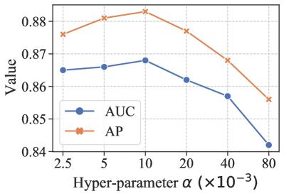
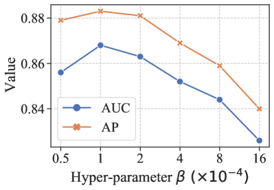
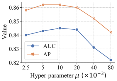
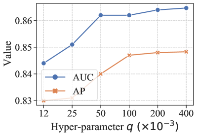
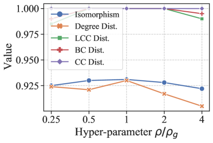
Figure 5: Results of hyper-parameter analysis on Cora dataset

6.2.4 Effectiveness of Black-box attack

TABLE IV: Performance of Black-box attacks. We report the attack AUC ($\%$), AP ($\%$), AQ, and AT of two black-box attack methods. We also show the results of white-box GraphMI for reference.

Dataset	Method	AUC	AP	AQ	AT (s)
Cora	GraphMI	86.8	88.3	-	29.0
	GE	84.5	86.2	10,000	760.9
	RL-GraphMI	80.5	79.2	270,800	5870.6
Citeseer	GraphMI	87.8	88.5	-	30.1
	GE	86.5	87.3	10,000	787.6
	RL-GraphMI	87.5	88.2	473,200	6082.7
Polblogs	GraphMI	79.3	79.7	-	19.8
	GE	69.0	66.4	10,000	671.2
	RL-GraphMI	54.6	51.2	1,902,500	19102.5
USA	GraphMI	80.6	81.3	-	28.4
	GE	66.7	66.9	10,000	780.4
	RL-GraphMI	55.2	53.1	1,359,900	11044.1
Brazil	GraphMI	86.6	88.8	-	12.5
	GE	78.2	79.3	10,000	571.6
	RL-GraphMI	74.9	76.3	103,800	3389.3

In Table IV, we show the attack performance of Gradient Estimation (abbreviated as GE) and RL-GraphMI. We also list the results of GraphMI for reference. Generally, GA and RL-GraphMI can achieve competitive attack performance in the black-box setting. For example, GE and RL-GraphMI achieve 86.5$\%$ and 87.5$\%$ attack AUC on Citesser, which are only 1.3 and 0.3 percent points less than the white box attack GraphMI. We also observe that RL-GraphMI has better performance on datasets with fewer nodes and edges such as Brazil, Cora, and Citesser because the agent has a smaller searching space. Compared with RL-GraphMI, gradient estimation has less average time (AT) and average queries (AQ), which makes it a more efficient choice for the black-box attack.

Theorem 2 analyzes the convergence property of the gradient estimation method. Here, we conduct experiments to verify the theorem of convergence. Fig. 6 shows that the L2 norm estimated gradient converges to 0 with respect to iterations. Therefore, Theorem 2 is verified empirically.

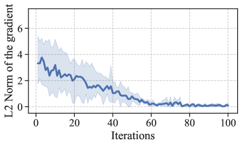
Figure 6: Convergence of the gradient estimation. We show the means and $95\%$ confidence intervals.

6.2.5 Ablation Study and Hyper-parameter Analysis

TABLE V: Ablation study of auto-encoder module ($\%$).

Dataset	w/ auto-encoder module	AUC	AP
Cora	Yes	86.8	88.3
	No	82.5	81.7
Citeseer	Yes	87.8	88.5
	No	85.6	86.2
Polblogs	Yes	79.3	79.7
	No	70.1	70.4

Here we conduct ablation studies to show the impact of the auto-encoder module on the attack performance in Table V. We can observe that with the auto-encoder module, GraphMI achieves the best results over all three datasets. This is because the node embeddings generated by the graph auto-encoder module fully exploit the information of node attributes, graph topology, and the target model. The similarity of such node embeddings could indicate the existence of edges more precisely.

We also explore the sensitivity of hyper-parameters $\alpha$, $\beta$, $\mu$, $q$, and $\rho$. In Fig 5, we alter the value of hyperparameters to see how they affect the attack performance. Specifically, we vary $\alpha$ from 0.00025 to 0.008, $\beta$ from 0.00005 to 0.0016, $\mu$ from 0.0025 to 0.08, $q$ from 12 to 400, and $\rho/\rho_{g}$ from 0.25 to 4 in a log scale of base 2. As we can observe, the attack performance of GraphMI can be boosted by choosing proper values for $\alpha$ and $\beta$. For the hyperparameters in the black-box attack, gradient estimation has the optimal performance at $\mu=0.01$. This may be explained by the fact that too large step leads to biased gradient estimation while too small step incurs relatively more random noise. Gradient estimation can achieve better performance with larger $q$ due to more accurate estimation. Considering the efficiency, we choose $q=100$ as the default setting in experiments. In Fig 5(e), we show how the influence of estimated graph density $\rho$ and $\rho_{g}$ is the ground truth density. We can observe that our attack is generally robust to $\rho$: GraphMI achieves over 0.90 on all metrics with different estimated graph density $\rho$. What’s more, the optimal performance of GraphMI is achieved when $\rho=\rho_{g}$.

7 Defending against GraphMI

In this section, we introduce and evaluate two defense methods against GraphMI: one is to train GNNs with differential privacy and the other is to preprocess the graph by perturbing edges.

7.1 Defense Performance of Differentail Privacy

Differential privacy (DP) is one general approach for protecting privacy. More formally:

Definition 1

(($\epsilon,\delta$)-differential privacy) A randomized mechanism $M$ with domain $\mathcal{R}$ and output $\mathcal{S}$ satisfies ($\epsilon,\delta$)-differential privacy if for any neighboring datasets $D,D^{\prime}\in\mathcal{R}$, which differ by at most one record and for any subsets of outputs $S$ it holds that:

$$Pr[M(D)\in S]\leq e^{\epsilon}Pr[M(D^{\prime})\in S]+\delta,$$ (26)

where $\epsilon$ is the privacy budget and $\delta$ denotes the failure probability.

Here, we investigate the impact of differential privacy on three attacks. $(\epsilon,\delta)$ - DP is ensured by adding Gaussian noise to the clipped gradients in each training iteration [1]. In experiments, $\delta$ is set to $10^{-5}$ and the noise scale is varied to obtain target GNN models with different $\epsilon$ from 1.0 to 10.0. The GraphMI attack performance and their model utility are presented in Table VI. As the privacy budget $\epsilon$ drops, the performance of GraphMI attack deteriorates at the price of a huge utility drop. For example, the trained GNN model only retains a node classification accuracy of 0.48 when the GraphMI attack AUC is decreased to 0.60. Generally, enforcing DP on target models cannot prevent GraphMI attack while preserving decent model utility.

7.2 Defense Performance of Graph Preprocessing

Here we propose one new defense method based on graph preprocessing. Instead of adding noise in GNN model training, our method pre-processes the training graph to ”hide” real edges from model inversion. Specifically, we apply the following three strategies in training graph pre-processing:

Randomly rewiring: For the exisiting edge ($v_{i},v_{j}$) in the training graph, with probability $p$, the rewiring operation deletes the existing edge between nodes $v_{i}$ and $v_{j}$, while adding an edge to connect nodes $v_{i}$ and $v_{k}$ or $v_{j}$ and $v_{k}$ ($k\neq i$ or $j$).

Adding new edges: Specifically, to preserve utility of trained GNN model, we add pseudo edges with high feature similarity. Compared with convolutional neural networks for image data, graph neural network generally has fewer layers and parameters. GNN models essentially aggregate features according to graph structure. Previous work on graph adversarial learning [53] suggests that adding edges with low feature similarity will severely undermines the utility of GNN model in node classification. Compared with adding edges randomly in the training graph, adding edges with high feature similarity helps preserve model utility.

Randomly flipping edges: For each entry in the adjacency matrix, with probability $1-p~{}(p\in(0,1])$ we keep it the same as the original graph; with probability $p$, we sample it randomly from $Bern(1/2)$. $Bern(\cdot)$ is the Bernoulli distribution. Such perturbation is proven to be $\epsilon$-edge level differential privacy ($\epsilon=ln(\frac{2}{p}-1)$) [52].

TABLE VI: The performance of the GraphMI, GE and RL-GraphMI attack (AUC) against GCN trained with differential privacy on Cora dataset

Method	ACC	GraphMI	GE	RL-GraphMI
$\epsilon=1.0$	0.48	0.60	0.61	0.58
$\epsilon=5.0$	0.65	0.72	0.70	0.65
$\epsilon=10.0$	0.78	0.84	0.79	0.76
no DP	0.80	0.87	0.85	0.81

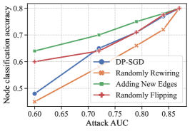
(a) GraphMI

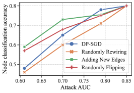
(b) GE

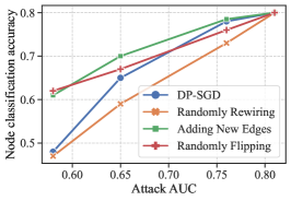
(c) RL-GraphMI

Figure 7: The trade-off curves between attack AUC and node classification accuracy on Cora dataset.

Figure 7 shows the trade-off between GNN utility and attack AUC of GraphMI, GE, and RL-GraphMI. Four defense strategies are shown, including DP-SGD and three graph pre-processing methods. Generally, all these defense methods can decrease the attack AUC at the price of node classification accuracy. Among the three pre-processing strategies, adding edges has the best defense performance. For instance, the trained GNN model has a classification accuracy of 0.64 when the attack AUC is decreased to 0.60 for GraphMI. This verifies our claim that adding edges with high feature similarity helps preserve model utility while defending against GraphMI attacks. On the other hand, randomly rewiring edges has a poor performance. The rewiring operation may link nodes with distinct labels or dissimilar features, which may damage the GNN model utility a lot.

7.3 Discussion

The defense results in Section 7.1 and Section 7.2 indicate that our graph model inversion attack is still effective even with differential privacy or graph preprocessing. There are several potential ways to strengthen the defense such as adversarial training and detection of adversarial queries in the black-box setting. We left them for future work.

8 Conclusion

In this paper, we conducted a systematic study on model inversion attacks against graph neural networks. We first presented GraphMI, a white-box attack specifically designed and optimized for extracting private graph-structured data from GNNs. Though GraphMI could effectively reconstruct the edges by exploiting the properties of graph and GNNs, it is infeasible in the black-box setting where the attacker is only allowed to query the GNN API and receive the classification results. Therefore, we extended GraphMI to the hard-label black-box setting and proposed two black-box attacks based on gradient estimation and reinforcement learning. Extensive experimental results showed its effectiveness on several state-of-the-art graph neural networks. Finally, we showed that imposing differential privacy on graph neural networks and graph preprocessing are not effective enough to protect privacy while preserving decent model utility.

This paper provided potential tools for investigating the privacy risks of deep learning models on graph-structured data. Interesting future directions include: 1) Design black-box attacks with better query efficiency; 2) Design countermeasures with a better trade-off between utility and privacy.

Zaixi Zhang received the BS degree from the department of gifted young, University of Science and Technology of China (USTC), China, in 2019. He is currently working toward the Ph.D. degree in the School of Computer Science and Technology at USTC. His main research interests include data mining, machine learning security and privacy, graph representation learning. He has published papers in referred conference proceedings, such as IJCAI, NeurIPS, KDD, and AAAI.

Qi Liu received the Ph.D. degree from University of Science and Technology of China (USTC), Hefei, China, in 2013. He is currently a Professor in the School of Computer Science and Technology at USTC. His general area of research is data mining and knowledge discovery. He has published prolifically in refereed journals and conference proceedings (e.g., TKDE, TOIS, KDD). He is an Associate Editor of IEEE TBD and Neurocomputing. He was the recipient of KDD’ 18 Best Student Paper Award and ICDM’ 11 Best Research Paper Award. He is a member of the Alibaba DAMO Academy Young Fellow. He was also the recipient of China Outstanding Youth Science Foundation in 2019.

Zhenya Huang recieved the B.E. degree from Shandong University, in 2014 and the Ph.D. degree from University of Science and Technology of China (USTC), in 2020. He is currently an associate researcher of the School of Computer Science and Technology, USTC. His main research interests include data mining, knowledge discovery, representation learning and intelligent tutoring systems. He has published more than 20 papers in refereed journals and conference proceedings including TKDE, TOIS, KDD, AAAI.

Hao Wang Hao Wang is currently an associate researcher of the School of Computer Science and Technology, USTC. His main research interests include data mining, representation learning, network embedding and recommender systems. He has published several papers in referred conference proceedings, such as TKDE, TOIS, NeurIPS, and KDD.

Chee-Kong Lee is a senior researcher at Tencent Quantum Lab. He obtained his undergraduate degree in physics from the National University of Singapore and PhD degree in theoretical chemistry from Massachusetts Institute of Technology (MIT). His research interests include quantum computing, computational chemistry, and applications of machine learning in chemistry and physics.

Enhong Chen (SM’07) is a professor and vice dean of the School of Computer Science at University of Science and Technology of China (USTC). He received the Ph.D. degree from USTC. His general area of research includes data mining and machine learning, social network analysis and recommender systems. He has published more than 100 papers in refereed conferences and journals, including IEEE Trans. KDE, IEEE Trans. MC, KDD, ICDM, NIPS, and CIKM. He was on program committees of numerous conferences including KDD, ICDM, SDM. He received the Best Application Paper Award on KDD-2008, the Best Student Paper Award on KDD-2018 (Research), the Best Research Paper Award on ICDM-2011 and Best of SDM-2015. His research is supported by the National Science Foundation for Distinguished Young Scholars of China. He is a senior member of the IEEE.

Appendix A Proof of Theorem 1

Theorem 1. $Adv(e_{i})\leq Adv(e_{j}),~{}\forall e_{i},e_{j}\in\mathcal{E}\cap\mathcal{I}(e_{i})\leq\mathcal{I}(e_{j})$ i.e. The adversary advantage is greater for edges with greater influence.

The proof is based on the lemma 1 from [54].

Lemma 1

Suppose the target model $f$ is trained on data distribution $p(\mathcal{X},\mathcal{Y})$. $\mathcal{X}=(x_{s},x_{ns})$, where $x_{s}$ and $x_{ns}$ denote the sensitive and non-sensitive part of feature respectively. The optimal adversary advantage is

$$P_{\mathcal{X}\sim p(\mathcal{X},\mathcal{Y})}[f(x_{s}=1,x_{ns})\neq f(x_{s}=0,x_{ns})].$$

Proof. In our graph setting, $x_{ns}$ refers to feature matrix $X$ and $x_{s}$ refers to edges. Set $P[f^{i}_{\theta}(A,X)=y_{i}]$ = $P_{f_{\theta}}(y_{i}~{}|~{}A,X)=p$; $P[f^{i}_{\theta}(A_{-e},X)=y_{i}]=P_{f_{\theta}}(y_{i}~{}|~{}A_{-e},X)=q$. For $f_{\theta}$, the prediction accuracy is higher with edge $e$, i.e. $q\leq p$. The adversary advantage is $Adv=[p(1-q)+q(1-p)]$. Through variable substitution ($x=p-q,y=p+q$), we have $Adv=(y+\frac{x^{2}-y^{2}}{2})$ and $\frac{\partial Adv}{\partial\mathcal{I}(e)}=\frac{\partial Adv}{\partial x}=p-q\geq 0$. Hence, $Adv(e_{i})\leq Adv(e_{j})$ if $e_{i},e_{j}\in\mathcal{E}$ and $\mathcal{I}(e_{i})\leq\mathcal{I}(e_{j})$. $\square$

Appendix B Proof of Theorem 2

Lemma 2

Define $\mathcal{L}_{\mu}(a)=\mathbb{E}_{v\in U_{b}}[\mathcal{L}_{attack}(a+\mu v)]$, where $U_{b}$ denotes a uniform distribution with respect to the unit Euclidean ball. We have:

$$\mathbb{E}[\hat{\nabla}\mathcal{L}_{attack}(a)]=\mathbb{E}_{u}[d/\mu\mathcal{L}_{attack}(a+\mu u)]=\nabla\mathcal{L}_{\mu}(a),$$ (27)

where $u$ is a vector picked uniformly at random from the Euclidean unit sphere. Under Assumption 1 and 2, $\mathcal{L}_{\mu}$ is $L_{1}$-Lipschitz continuous and has $L_{2}$-Lipschitz continuous gradient.

Proof. The proof can be found in [17] Lemma 1.

Lemma 3

If Assumption 2. holds and $\eta_{k}\in(0,1/L_{2})$, then the outputs $\{a_{t}\}_{t=0}^{T-1}$ from the gradient estimation algorithm satisfies:

$$\sum_{t=0}^{T-1}((2\eta_{t}-L_{2}\eta_{t}^{2})\mathbb{E}[\|P_{[0,1]}(a_{r},\hat{\nabla}\mathcal{L}_{attack}(a_{t}),\eta_{t})\|^{2}])$$ (28)

$$\leq\sum_{t=0}^{T-1}(2\eta_{t}\mathbb{E}[\|\hat{\nabla}\mathcal{L}_{attack}(a_{t})-\mathbb{E}[\hat{\nabla}\mathcal{L}_{attack}(a_{t})|a_{t}]\|^{2}])$$ (29)

$$+2\mu^{2}L_{2}+c_{2},$$ (30)

where $\mathbb{E}$ is taken with respect to all the randomness (e.g., random directions), $P_{[0,1]}$ is the gradient projection given by Equ. 14, and $c_{2}=2(f(a_{0})-f(a^{*}))$ ($a^{*}$ is the globally optimal solution).

Proof. The proof can be found in [33] Proposition 1.

Theorem 3

Suppose Assumption 1$\&$2 hold. If we randomly pick $a_{r}$, whose dimension is $d$, from $\{a_{t}\}_{t=0}^{T-1}$ with probability $P(r=t)=\frac{2\eta_{t}-L_{2}\eta_{t}^{2}}{\sum_{t=0}^{T-1}2\eta_{t}-L_{2}\eta_{t}^{2}}$ Then, we have the following bound on the convergence rate with $\eta_{t}=\mathcal{O}(\frac{1}{\sqrt{T}})$ and $\mu=\mathcal{O}(\frac{1}{\sqrt{dq}})$:

$$\mathbb{E}[\|P_{[0,1]}(a_{r},\hat{\nabla}\mathcal{L}_{attack}(a_{r}),\eta_{r})\|^{2}]=\mathcal{O}(\frac{1}{\sqrt{T}}+\frac{d+q}{q}),$$ (31)

where $P_{[0,1]}(a_{r},\hat{\nabla}\mathcal{L}_{attack}(a_{r}),\eta_{r})\coloneqq(1/\eta_{r})[a_{r}-P_{[0,1]}(a_{r}-\eta_{r}\hat{\nabla}\mathcal{L}_{attack}(a_{r}))$ is the rectified gradient.

Proof. Since $\mathbb{E}[\hat{\nabla}\mathcal{L}_{attack}(a_{t})|a_{t}]=\nabla\mathcal{L}_{\mu}(a_{t})$, we have:

$$\mathbb{E}[\|\hat{\nabla}\mathcal{L}_{attack}(a_{t})-\mathbb{E}[\hat{\nabla}\mathcal{L}_{attack}(a_{t})|a_{t}]\|^{2}]$$ (32)

$$=\mathbb{E}[\|\hat{\nabla}\mathcal{L}_{attack}(a_{t})-\nabla\mathcal{L}_{\mu}(a_{t})\|^{2}]$$ (33)

$$\leq\mathbb{E}[\|\hat{\nabla}\mathcal{L}_{attack}(a_{t})\|^{2}]$$ (34)

$$\leq\frac{(c_{1}d+4q)L_{1}^{2}}{4q},$$ (35)

where the final inequality comes from [33] Lemma 1. Based on Lemma 3, we have:

$$\sum_{t=0}^{T-1}((2\eta_{t}-L_{2}\eta_{t}^{2})\mathbb{E}[\|P_{[0,1]}(a_{r},\hat{\nabla}\mathcal{L}_{attack}(a_{t}),\eta_{t})\|^{2}])$$ (36)

$$\leq\frac{(c_{1}d+4q)L_{1}^{2}}{2q}\sum_{t=0}^{T-1}\eta_{t}+2\mu^{2}L_{2}+c_{2}.$$ (37)

If we sample $a_{r}$ from $\{a_{t}\}_{t=0}^{T-1}$ with the probability in Theorem 3, we can then obtain:

$$\mathbb{E}[\|P_{[0,1]}(a_{r},\hat{\nabla}\mathcal{L}_{attack}(a_{r}),\eta_{r})\|^{2}]$$ (38)

$$\leq\frac{(c_{1}d+4q)L_{1}^{2}\sum_{t=0}^{T-1}\eta_{t}}{2q\sum_{t=0}^{T-1}((2\eta_{t}-L_{2}\eta_{t}^{2})}+\frac{2\mu^{2}L_{2}+c_{2}}{\sum_{t=0}^{T-1}((2\eta_{t}-L_{2}\eta_{t}^{2})}.$$ (39)

If we choose $\eta_{t}=\frac{c_{\eta}}{\sqrt{T}}\in(0,1/L_{2})$, then the above inequality implies the convergence rate of $\mathcal{O}(\frac{1}{\sqrt{T}}+\frac{d+q}{q})$. $\square$

Appendix C Macro-level Graph Statistics

• Degree Distribution The degree distribution $P(k)$ of a graph is defined to be the fraction of nodes in the graph with degree $k$. It is widely used to characterize the graph statistics.

• Local Clustering Coefficient (LCC). The LCC of a node measures the closeness to its neighbors to form a cluster. It is primarily proposed to determine if a graph is a small-world network.

• Betweenness Centrality (BC). Betweenness centrality measures the node centralities based on the shortest paths. For every pair of nodes in a graph, there exists at least one shortest path among all possible paths, which contains the minimal the number of edges. The betweenness centrality for a certain node is defined as the number of these shortest paths that pass through the node.

• Closeness Centrality (CC). Closeness Centrality is another measure of node centrality. It is defined as the reciprocal of the sum of the length of the shortest paths between the node and all other nodes in the graph. Generally, the larger the CC of a node is, the closer it is to all other nodes.

References

- [1] M. Abadi, A. Chu, I. Goodfellow, H. B. McMahan, I. Mironov, K. Talwar, and L. Zhang. Deep learning with differential privacy. In CCS 2016, pages 308–318, 2016.
- [2] L. A. Adamic and N. Glance. The political blogosphere and the 2004 us election: divided they blog. In Proceedings of the 3rd international workshop on Link discovery, pages 36–43, 2005.
- [3] U. Aïvodji, S. Gambs, and T. Ther. Gamin: An adversarial approach to black-box model inversion. arXiv preprint arXiv:1909.11835, 2019.
- [4] J. Blocki, A. Blum, A. Datta, and O. Sheffet. The johnson-lindenstrauss transform itself preserves differential privacy. In 2012 IEEE 53rd Annual Symposium on Foundations of Computer Science, pages 410–419. IEEE, 2012.
- [5] J. Blocki, A. Blum, A. Datta, and O. Sheffet. Differentially private data analysis of social networks via restricted sensitivity. In Proceedings of the 4th conference on Innovations in Theoretical Computer Science, pages 87–96, 2013.
- [6] A. Bojchevski and S. Günnemann. Certifiable robustness to graph perturbations. NeurIPS, 2019.
- [7] K. M. Borgwardt, C. S. Ong, S. Schönauer, S. Vishwanathan, A. J. Smola, and H.-P. Kriegel. Protein function prediction via graph kernels. Bioinformatics, 21(suppl_1):i47–i56, 2005.
- [8] H. Chang, Y. Rong, T. Xu, W. Huang, H. Zhang, P. Cui, W. Zhu, and J. Huang. A restricted black-box adversarial framework towards attacking graph embedding models. In AAAI, volume 34, pages 3389–3396, 2020.
- [9] J. Chen, X. Lin, Z. Shi, and Y. Liu. Link prediction adversarial attack via iterative gradient attack. IEEE Transactions on Computational Social Systems, 7(4):1081–1094, 2020.
- [10] J. Chen, Y. Wu, X. Xu, Y. Chen, H. Zheng, and Q. Xuan. Fast gradient attack on network embedding. arXiv preprint arXiv:1809.02797, 2018.
- [11] H. Dai, H. Li, T. Tian, X. Huang, L. Wang, J. Zhu, and L. Song. Adversarial attack on graph structured data. In ICML, pages 1115–1124, 2018.
- [12] Q. Dai, X. Shen, L. Zhang, Q. Li, and D. Wang. Adversarial training methods for network embedding. In WWW, pages 329–339, 2019.
- [13] V. Duddu, A. Boutet, and V. Shejwalkar. Quantifying privacy leakage in graph embedding. arXiv preprint arXiv:2010.00906, 2020.
- [14] C. Dwork, A. Roth, et al. The algorithmic foundations of differential privacy. Found. Trends Theor. Comput. Sci., 9(3-4):211–407, 2014.
- [15] W. Fan, Y. Ma, Q. Li, J. Wang, G. Cai, J. Tang, and D. Yin. A graph neural network framework for social recommendations. TKDE, 2020.
- [16] F. Feng, X. He, J. Tang, and T.-S. Chua. Graph adversarial training: Dynamically regularizing based on graph structure. TKDE, 2019.
- [17] A. D. Flaxman, A. T. Kalai, and H. B. McMahan. Online convex optimization in the bandit setting: gradient descent without a gradient. 2005.
- [18] M. Fredrikson, S. Jha, and T. Ristenpart. Model inversion attacks that exploit confidence information and basic countermeasures. In SIGSAC, pages 1322–1333, 2015.
- [19] M. Fredrikson, E. Lantz, S. Jha, S. Lin, D. Page, and T. Ristenpart. Privacy in pharmacogenetics: An end-to-end case study of personalized warfarin dosing. In USENIX Security, pages 17–32, 2014.
- [20] X. Gao, B. Jiang, and S. Zhang. On the information-adaptive variants of the admm: an iteration complexity perspective. Journal of Scientific Computing, 76(1):327–363, 2018.
- [21] J. Gilmer, S. S. Schoenholz, P. F. Riley, O. Vinyals, and G. E. Dahl. Neural message passing for quantum chemistry. In ICML, pages 1263–1272, 2017.
- [22] W. Hamilton, Z. Ying, and J. Leskovec. Inductive representation learning on large graphs. In NeurIPS, pages 1024–1034, 2017.
- [23] M. Hay, C. Li, G. Miklau, and D. Jensen. Accurate estimation of the degree distribution of private networks. In ICDM, pages 169–178. IEEE, 2009.
- [24] X. He, J. Jia, M. Backes, N. Z. Gong, and Y. Zhang. Stealing links from graph neural networks. In USENIX Security, 2021.
- [25] X. He, J.-Y. Jia, M. Backes, N. Gong, and Y. Zhang. Stealing links from graph neural networks. In USENIX Security, 2021.
- [26] I.-C. Hsieh and C.-T. Li. Netfense: Adversarial defenses against privacy attacks on neural networks for graph data. TKDE, 2021.
- [27] D. Jin, Z. Yu, C. Huo, R. Wang, X. Wang, D. He, and J. Han. Universal graph convolutional networks. NeurIPS, 34, 2021.
- [28] W. Jin, Y. Li, H. Xu, Y. Wang, and J. Tang. Adversarial attacks and defenses on graphs: A review and empirical study. arXiv preprint arXiv:2003.00653, 2020.
- [29] T. N. Kipf and M. Welling. Variational graph auto-encoders. Bayesian Deep Learning Workshop (NeurIPS 2016), 2016.
- [30] T. N. Kipf and M. Welling. Semi-supervised classification with graph convolutional networks. ICLR, 2017.
- [31] J. Li, T. Xie, C. Liang, F. Xie, X. He, and Z. Zheng. Adversarial attack on large scale graph. TKDE, 2021.
- [32] D. Lim, F. Hohne, X. Li, S. L. Huang, V. Gupta, O. Bhalerao, and S. N. Lim. Large scale learning on non-homophilous graphs: New benchmarks and strong simple methods. NeurIPS, 34, 2021.
- [33] S. Liu, X. Li, P.-Y. Chen, J. Haupt, and L. Amini. Zeroth-order stochastic projected gradient descent for nonconvex optimization. In GlobalSIP, pages 1179–1183. IEEE, 2018.
- [34] X. Liu, S. Si, X. Zhu, Y. Li, and C.-J. Hsieh. A unified framework for data poisoning attack to graph-based semi-supervised learning. NeurIPS, 2019.
- [35] J. Ma, S. Ding, and Q. Mei. Towards more practical adversarial attacks on graph neural networks. NeurIPS, 33:4756–4766, 2020.
- [36] Y. Ma, S. Wang, T. Derr, L. Wu, and J. Tang. Graph adversarial attack via rewiring. page 1161–1169, 2021.
- [37] V. Mnih, K. Kavukcuoglu, D. Silver, A. A. Rusu, J. Veness, M. G. Bellemare, A. Graves, M. Riedmiller, A. K. Fidjeland, G. Ostrovski, et al. Human-level control through deep reinforcement learning. Nature, 518(7540):529–533, 2015.
- [38] J. Mu, B. Wang, Q. Li, K. Sun, M. Xu, and Z. Liu. A hard label black-box adversarial attack against graph neural networks. In CCS, pages 108–125, 2021.
- [39] L. F. Ribeiro, P. H. Saverese, and D. R. Figueiredo. struc2vec: Learning node representations from structural identity. In SIGKDD, pages 385–394, 2017.
- [40] K. Riesen and H. Bunke. Iam graph database repository for graph based pattern recognition and machine learning. In Joint IAPR International Workshops on SPR and SSPR, pages 287–297. Springer, 2008.
- [41] M. Rigaki and S. Garcia. A survey of privacy attacks in machine learning. arXiv preprint arXiv:2007.07646, 2020.
- [42] P. Sen, G. Namata, M. Bilgic, L. Getoor, B. Galligher, and T. Eliassi-Rad. Collective classification in network data. AI magazine, 29(3):93–93, 2008.
- [43] O. Shamir. An optimal algorithm for bandit and zero-order convex optimization with two-point feedback. The Journal of Machine Learning Research, 18(1):1703–1713, 2017.
- [44] N. Shervashidze, P. Schweitzer, E. J. Van Leeuwen, K. Mehlhorn, and K. M. Borgwardt. Weisfeiler-lehman graph kernels. Journal of Machine Learning Research, 12(9), 2011.
- [45] R. Shokri, M. Stronati, C. Song, and V. Shmatikov. Membership inference attacks against machine learning models. In 2017 IEEE Symposium on Security and Privacy, pages 3–18. IEEE, 2017.
- [46] L. Sun, Y. Dou, C. Yang, J. Wang, P. S. Yu, L. He, and B. Li. Adversarial attack and defense on graph data: A survey. arXiv preprint arXiv:1812.10528.
- [47] Y. Sun, S. Wang, X. Tang, T.-Y. Hsieh, and V. Honavar. Non-target-specific node injection attacks on graph neural networks: A hierarchical reinforcement learning approach. In WWW, 2020.
- [48] F. Tramèr, F. Zhang, A. Juels, M. K. Reiter, and T. Ristenpart. Stealing machine learning models via prediction apis. In USENIX, pages 601–618, 2016.
- [49] P. Veličković, G. Cucurull, A. Casanova, A. Romero, P. Lio, and Y. Bengio. Graph attention networks. ICLR, 2018.
- [50] B. Wang and N. Z. Gong. Attacking graph-based classification via manipulating the graph structure. In SIGSAC, 2019.
- [51] B. Wu, X. Yang, S. Pan, and X. Yuan. Model extraction attacks on graph neural networks: Taxonomy and realization. arXiv preprint arXiv:2010.12751, 2020.
- [52] F. Wu, Y. Long, C. Zhang, and B. Li. Linkteller: Recovering private edges from graph neural networks via influence analysis. S&P, 2021.
- [53] H. Wu, C. Wang, Y. Tyshetskiy, A. Docherty, K. Lu, and L. Zhu. Adversarial examples on graph data: Deep insights into attack and defense. IJCAI, 2019.
- [54] X. Wu, M. Fredrikson, S. Jha, and J. F. Naughton. A methodology for formalizing model-inversion attacks. In 2016 IEEE 29th CSF, pages 355–370. IEEE, 2016.
- [55] J. Xu, J. Chen, S. You, Z. Xiao, Y. Yang, and J. Lu. Robustness of deep learning models on graphs: A survey. AI Open, 2:69–78, 2021.
- [56] K. Xu, H. Chen, S. Liu, P.-Y. Chen, T.-W. Weng, M. Hong, and X. Lin. Topology attack and defense for graph neural networks: An optimization perspective. IJCAI, 2019.
- [57] S. Yeom, I. Giacomelli, M. Fredrikson, and S. Jha. Privacy risk in machine learning: Analyzing the connection to overfitting. In 2018 IEEE 31st CSF, pages 268–282. IEEE, 2018.
- [58] M. Zhang, S. Wu, M. Gao, X. Jiang, K. Xu, and L. Wang. Personalized graph neural networks with attention mechanism for session-aware recommendation. TKDE, 2020.
- [59] X. Zhang, L. Zhang, B. Jin, and X. Lu. A multi-view confidence-calibrated framework for fair and stable graph representation learning. In 2021 IEEE International Conference on Data Mining (ICDM), 2021.
- [60] Y. Zhang, R. Jia, H. Pei, W. Wang, B. Li, and D. Song. The secret revealer: generative model-inversion attacks against deep neural networks. In CVPR, pages 253–261, 2020.
- [61] Z. Zhang, M. Chen, M. Backes, Y. Shen, and Y. Zhang. Inference attacks against graph neural networks. In USENIX Security, volume 2022, page 13, 2021.
- [62] Z. Zhang, P. Cui, and W. Zhu. Deep learning on graphs: A survey. TKDE, 2020.
- [63] Z. Zhang, Q. Liu, Z. Huang, H. Wang, C. Lu, C. Liu, and E. Chen. Graphmi: Extracting private graph data from graph neural networks. In IJCAI, pages 3749–3755, 2021.
- [64] Z. Zhang, Q. Liu, H. Wang, C. Lu, and C.-K. Lee. Motif-based graph self-supervised learning for molecular property prediction. NeurIPS, 34, 2021.
- [65] D. Zügner, A. Akbarnejad, and S. Günnemann. Adversarial attacks on neural networks for graph data. In SIGKDD, pages 2847–2856, 2018.
- [66] D. Zügner and S. Günnemann. Adversarial attacks on graph neural networks via meta learning. ICLR, 2019.