SRFeat: Learning Locally Accurate and Globally Consistent
Non-Rigid Shape Correspondence

Abstract

In this work, we present a novel learning-based framework that combines the local accuracy of contrastive learning with the global consistency of geometric approaches, for robust non-rigid matching. We first observe that while contrastive learning can lead to powerful point-wise features, the learned correspondences commonly lack smoothness and consistency, owing to the purely combinatorial nature of the standard contrastive losses. To overcome this limitation we propose to boost contrastive feature learning with two types of smoothness regularization that inject geometric information into correspondence learning. With this novel combination in hand, the resulting features are both highly discriminative across individual points, and, at the same time, lead to robust and consistent correspondences, through simple proximity queries. Our framework is general and is applicable to local feature learning in both the 3D and 2D domains. We demonstrate the superiority of our approach through extensive experiments on a wide range of challenging matching benchmarks, including 3D non-rigid shape correspondence and 2D image keypoint matching.

1 Introduction

Finding accurate correspondences across geometric objects is a fundamental task in a wide range of computer vision and graphics problems, such as object tracking, registration, texture transfer, and statistical shape analysis [99, 24, 10], among many others. The presence of significant variations in 3D or 2D geometric objects, including rigid and non-rigid transformations, makes it challenging to develop a single unified theoretical deformation model for robust matching [87, 82]. Earlier approaches to computing correspondences heavily relied on hand-crafted features and pipelines [87]. In more recent years, there has been a growing body of literature advocating the use of deeply learned features that demonstrate superior matching performance over axiomatic approaches [31, 77, 72, 18, 25].

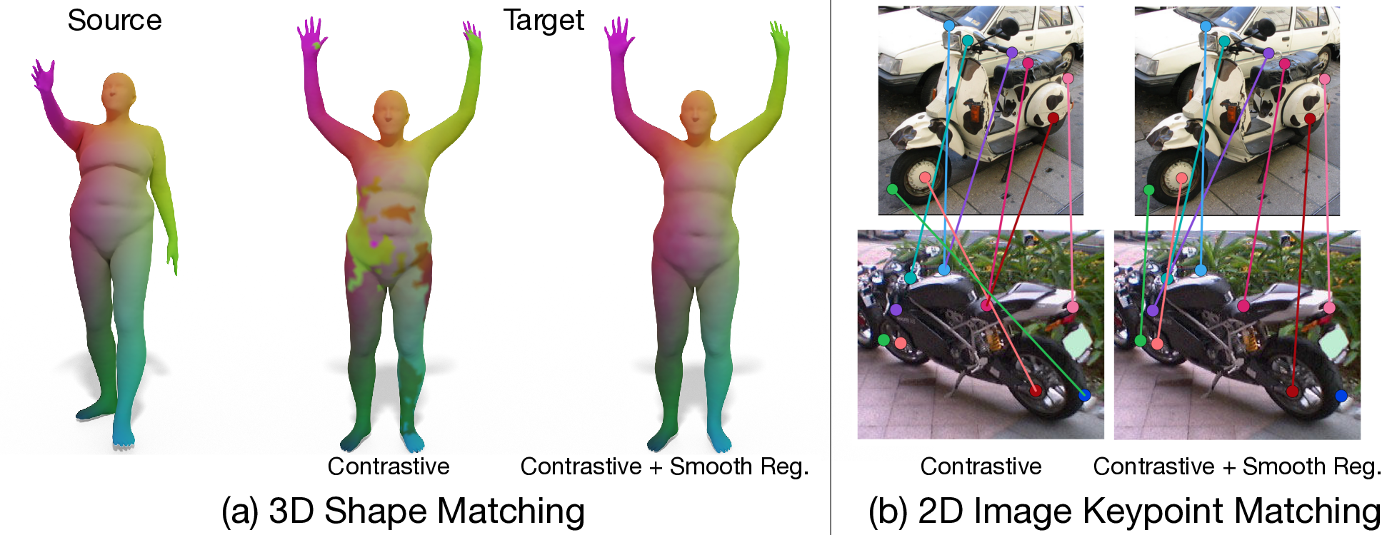
Figure 1: We propose a smoothness-regularized contrastive learning approach for local feature learning, which leads to more accurate, consistent correspondences. (a) Dense non-rigid 3D shape matching via learned features on the FAUST dataset [10]. Correspondence is visualized by color transfer. (b) 2D image keypoint matching through node-wise features on the PASCAL VOC dataset [30]. Ground-truth corresponding keypoints have the same node color.

In this work, we focus on learning discriminative local features that can robustly identify each point on a given geometric object for correspondence. Given such local features for a pair of objects, finding point-wise correspondences simply reduces to proximity queries in the learned feature space [37]. However, it is not easy to endow local features with descriptiveness and robustness for geometric objects potentially undergoing arbitrary deformations.

Contrastive learning is a popular approach to training local feature extractors, for example, in the task of 3D rigid point cloud registration [98, 23, 34, 52, 6, 18, 94]. The wide adoption of contrastive learning lies in the fact that it is extremely generic, as also actively studied in 2D visual representation learning [41, 15, 35, 31], and thus can be applicable to arbitrary 3D or 2D shape classes. On the other hand, this learning paradigm is inherently based on computing correspondences across individual points by comparing their local features. As a result, while the learned features can be very discriminative, the overall quality of the correspondences can suffer and especially lack smoothness and consistency [16, 5], as shown in Fig. 1 (a). Thus, so far, there is limited success in training local features purely with contrastive learning for direct nearest-neighbor matching, e.g., for non-rigid shape correspondence [22].

Motivated by the above discussion, we introduce a novel smoothness-regularized contrastive learning approach, enabling robust feature-based matching of deformable objects. Specifically, we boost the contrastive loss at training time (e.g., the PointInfoNCE loss [94]) with powerful smoothness regularization terms that promote the overall consistency of the learned point-wise features. Our resulting approach, which we call SRFeat, enjoys the advantages of contrastive learning, by obtaining highly discriminative local features, which can be accurately matched via direct feature proximity queries. Moreover, owing to the smoothness promotion, the resulting local features are strongly regularized, thus leading to overall smooth and consistent correspondences even without any post-processing (Fig. 1 (a)).

We initiate the study of smoothness regularization for contrastive learning, specifically, for deformable shape correspondence. We propose two implementation variants for the smoothness regularization at training time (Sec. 3.2): (1) a Dirichlet energy loss that penalizes discontinuities in the feature space and (2) a spectral loss that evaluates the correspondence matrices in the spectral domain. We demonstrate the superior performance of SRFeat through a comprehensive set of experiments on diverse non-rigid shape matching benchmarks [10, 1, 58, 100]. At test time, we compute correspondences between non-rigid shapes by nearest-neighbor queries with the learned features, in contrast to the state-of-the-art methods [25, 29] that typically require the Laplacian basis computation and a test-time correspondence optimization in the spectral domain.

In addition, our smoothness regularization is remarkably generic and can be easily incorporated into other modern contrastive feature learning frameworks in other domains (e.g., images), and thus we position SRFeat as a general local feature learning approach. To demonstrate the wide applicability, as shown in Fig. 1 (b), we apply SRFeat to the 2D image domain for keypoint matching [30, 31], bringing significant improvement over existing methods.

In a nutshell, the main contributions of our work are as follows: (1) We introduce a novel generic smoothness regularization to the contrastive feature learning framework, substantially improving the smoothness and consistency of correspondences found by local features; (2) We establish a link between contrastive learning and spectral (functional map-based) shape correspondence methods by relating ways in which these approaches operate on the computed correspondence matrices; (3) We show that contrastive feature learning combined with smoothness regularization yields superior matching performance over existing methods on widely adopted non-rigid shape benchmarks; (4) We demonstrate the strong generality of SRFeat to the 2D domain for tackling matching problems on real-world image data. Our code and data are publicly available.

2 Related Work

Contrastive Learning  Contrastive learning has recently received significant research attention as a powerful representation learning paradigm for both 2D and 3D data. In the 2D domain, contrastive learning is widely used for unsupervised learning of 2D representations [64, 41, 15, 35, 31, 20]. Meanwhile, researchers also actively investigate this generic learning paradigm for 3D geometric data. For example, PointContrast [94] and its follow-up work [42] perform local feature contrasting at the point level between two transformed 3D scene fragments. The learned feature representation is shown to be useful in downstream 3D tasks like segmentation and detection [21]. Besides, there also exist recent works performing the contrasting at the local patch level [26], object instance level [68], global scene level [46], or both the shape and point levels [90]. Our work, related to [94, 31], focuses on learning local features for robustly identifying individual points on deformable geometric objects for correspondence. To boost the performance of contrastive feature learning, we propose smoothness regularization and show its utility in a wide range of matching problems.

Shape Matching  Shape matching is a key problem in 3D shape analysis and has been extensively studied in recent decades [37, 87, 9, 38, 13, 72, 22]. Earlier works focused primarily on hand-crafted 3D local features for matching, including both extrinsic [47, 33, 75, 74, 76] and intrinsic [81, 4] descriptors. In recent years, research focus has shifted to learned local features for better robustness in matching, for example, in the task of point cloud registration [98, 23, 34, 92, 95, 52, 2, 6, 5]. For non-rigid shapes, a common approach to computing correspondence is to leverage spectral information, e.g., using the functional map framework [65] and its follow-up works [50, 43, 14, 71, 62, 69, 44]. In particular, several recent approaches [54, 73, 29, 36, 25, 3] have built upon this framework by advocating learned probe functions. There also exist a few works [57, 61] exploring surface CNNs with the contrastive loss proposed by Hadsell et al. [39] to learn features for non-rigid shapes. However, the performance of such approaches on dense shape correspondence was not shown to be comparable to that of the spectral methods.

Our SRFeat framework differs from the above state-of-the-art non-rigid shape matching approaches [25, 3], which require the spectral basis computation and optimization in the spectral domain at test time. Instead, our approach achieves superior matching performance by directly matching local features, learned via our smoothness-regularized contrastive learning strategy.

Image Keypoint Matching  Image matching is a well studied area in computed vision, and a full review is beyond the scope of this work. We refer the interested readers to recent surveys [56, 51, 8] for a more in-depth discussion. Finding correspondences between 2D images is a difficult problem, due to the potentially strong differences in appearance, and ambiguities introduced by repeating patterns. Classical methods for solving this problem were based on handcrafted features such as [55, 60, 84]. Strategies such as ratio test [55] or mutual check were used to reduce ambiguous matches. Recent methods are based on trainable feature descriptors extracted by convolutional neural networks (CNNs). They either operate on patches extracted by handcrafted feature detectors and produce a sparse set of descriptors [80, 88, 7, 79], or involve end-to-end methods combining detection and description [96, 63, 19]. Several methods have been proposed for producing consistent matches [70, 97, 91, 31]. DGMC [31] tackles this problem by constructing a graph for image keypoints and seeking consensus of matches in local neighborhoods using a synchronous message passing network, while using a standard contrastive loss for training. In this work, we investigate the strong generality of our smoothness regularization in the image keypoint matching task, showing its significant improvement to the contrastive learning used in [31].

3 Method

3.1 Background

Contrastive learning [39, 64] is a widely adopted approach to learning informative representations for 3D [94] and 2D [41, 31] vision understanding tasks. Specifically, the PointInfoNCE loss introduced in [94] was formulated on individual points to train 3D local features for rigid alignment. Given a pair of point clouds $\mathcal{P}_{1}$ and $\mathcal{P}_{2}$ with $n_{1}$ and $n_{2}$ points, respectively, below we re-write this contrastive loss using a feature similarity matrix $\mathbf{\Pi}\in\mathbb{R}^{n_{1}\times n_{2}}$, as this will be useful to establish the link to spectral approaches in Sec. 3.2. Let $\mathbf{f}_{1}^{i},\ \mathbf{f}_{2}^{j}\in\mathbb{R}^{d}$ denote $d$-dimensional features for the $i^{\text{th}}$ point in $\mathcal{P}_{1}$ and $j^{\text{th}}$ point in $\mathcal{P}_{2}$, respectively. The similarity matrix $\mathbf{\Pi}$ is then constructed as:

$$\mathbf{\Pi}^{i,j}=\dfrac{\exp\big{(}s(\mathbf{f}_{1}^{i},\mathbf{f}_{2}^{j})/\tau\big{)}}{\sum_{k=1}^{n_{2}}\exp\big{(}s(\mathbf{f}_{1}^{i},\mathbf{f}_{2}^{k})/\tau\big{)}},$$ (1)

$$s(\mathbf{x},\mathbf{y})=\mathbf{x}\cdot\mathbf{y},$$ (2)

where $s(\cdot,\cdot)$ is the similarity measurement between two feature vectors, and $\tau$ is a temperature hyper-parameter. Eq. 1 can be thought of as applying row-wise softmax to the pairwise similarity in Eq. 2. The PointInfoNCE loss is then defined as:

$$\mathcal{L}_{\text{c}}=-\sum_{i}\log\big{(}\mathbf{\Pi}^{i,\text{GT}(i)}\big{)}.$$ (3)

Here $\text{GT}(i)$ denotes the ground-truth correspondence. In [94], $\mathcal{P}_{1}$ and $\mathcal{P}_{2}$ are partially overlapped and thus only points sparsely sampled in the overlap region are considered in the above formulation.

Another example of contrastive learning is its application to the graph matching problem [91], aiming at establishing correspondences between the nodes of two input graphs, such as for 2D image keypoint matching [30]. The training loss used in the deep graph matching consensus (DGMC) framework [31] has a similar formulation to Eq. 3.

Interestingly, as we demonstrate in Sec. 4.1, the PointInfoNCE loss alone, when used in conjunction with a recent powerful feature extractor [78], can already lead to point-wise features that induce competitive correspondences on near-isometric 3D shape benchmarks. This result suggests that it is viable to establish correspondences between non-rigid shape pairs by simple proximity queries in the feature space, differently from common approaches [11, 93, 78, 25] that are either based on predicting vertex ids of some reference shape or use test time optimization. However, we also find that using the PointInfoNCE loss alone can lead to discontinuous maps, especially in the presence of non-isometries, due to the issues discussed below.

Formulation Issues  Despite the generality of contrastive learning, fundamentally the loss in Eq. 3 only considers whether individual point correspondences are correct or not, without exploiting any geometric structure of the shapes. This means that incorrect predictions are penalized equally regardless of whether they are close to the ground-truth match or not. More broadly, contrastive learning does not consider structural properties of the underlying map, such as continuity or smoothness. Such properties emerge when one considers either relations between learned feature embeddings of points on the shapes, or analyzing the map as a whole [54, 73, 25]. To mitigate the issues, we propose to use simple yet powerful regularization by promoting smoothness in the learned local features, while maintaining the simplicity and advantages of contrastive learning.

3.2 Smoothness-Regularized Feature Learning

Our goal is to train a robust feature extraction network that would enable shape matching via simple proximity queries between features at different points. We base our approach, SRFeat, on the generic contrastive learning framework (Sec. 3.1), and propose to boost contrastive feature learning with smoothness regularization. In what follows, we first instantiate the formulations of smoothness regularization in the 3D domain and then discuss the generalization to the 2D domain (Sec. 3.3).

Let us first define the notation for feature extraction. Suppose we are given a pair of non-rigid shapes $\mathcal{S}_{1}$ and $\mathcal{S}_{2}$ with ground-truth correspondences. The shapes are represented as graphs (i.e., triangle meshes) and contain $n_{1}$ and $n_{2}$ vertices, respectively. We denote our feature extractor as $\mathcal{F}_{\Theta}$, where $\Theta$ represents the trainable network parameters. We obtain point-wise features for each shape by forwarding it to the feature extractor $\mathcal{F}_{\Theta}$. Specifically, let $\mathbf{G}_{1}=\mathcal{F}_{\Theta}(\mathcal{S}_{1})$ and $\mathbf{G}_{2}=\mathcal{F}_{\Theta}(\mathcal{S}_{2})$ denote the sets of resulting $d$-dimensional features for the two shapes, respectively, where $\mathbf{G}_{1}\in\mathbb{R}^{n_{1}\times d}$ and $\mathbf{G}_{2}\in\mathbb{R}^{n_{2}\times d}$. We refer to each column of the feature matrices as a real-valued feature function defined on the vertices of the corresponding shape.

Our SRFeat framework is conceptually simple and is illustrated in Fig. 2. SRFeat trains the feature extractor $\mathcal{F}_{\Theta}$ with a novel training loss $\mathcal{L}$ that combines contrastive learning with smoothness regularization:

$$\mathcal{L}=\mathcal{L}_{\text{c}}+\lambda\mathcal{L}_{\text{s}},$$ (4)

where $\lambda$ is a weighting hyper-parameter. The first term $\mathcal{L}_{\text{c}}$ is the contrastive loss (Sec. 3.1) that promotes small feature distance between corresponding points and large feature distance between non-corresponding ones. The second term $\mathcal{L}_{\text{s}}$ is the smoothness regularization loss for $\mathbf{G}_{1}$ and $\mathbf{G}_{2}$, exploiting geometric information in the input shapes. We propose two variants for $\mathcal{L}_{\text{s}}$, as detailed below.

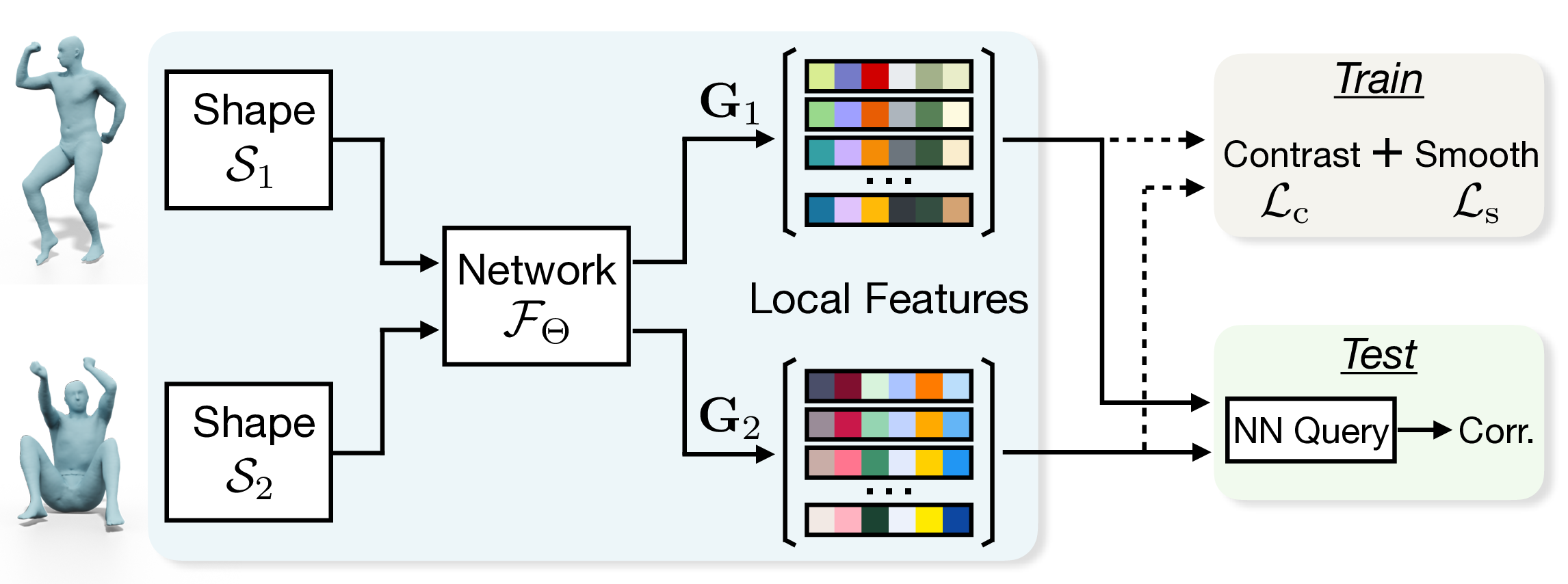
Figure 2: Overview of our smoothness-regularized contrastive learning framework. To train the extracted local features $\mathbf{G}_{1}$ and $\mathbf{G}_{2}$ by the network $\mathcal{F}_{\Theta}$, we augment the contrastive loss $\mathcal{L}_{\text{c}}$ with a smoothness regularization loss $\mathcal{L}_{\text{s}}$. At test time, correspondences between the input deformable shapes are found by nearest-neighbor query between $\mathbf{G}_{1}$ and $\mathbf{G}_{2}$.

Dirichlet Energy Loss  To regularize the smoothness of the learned local features, we consider the feature functions defined on the shapes (i.e., each column of $\mathbf{G}_{1}$ and $\mathbf{G}_{2}$). Our first loss is based on the Dirichlet energy [66], which intuitively measures how smooth those functions are. Given a real-valued function $g:\mathcal{S}\rightarrow\mathbb{R}$ on the shape $\mathcal{S}$, the Dirichlet energy is defined as:

$$\mathcal{E}_{\text{d}}(g)=\int_{\mathcal{S}}\|\nabla g\|^{2}dA.$$ (5)

In the discrete case, the Dirichlet energy can be computed as:

$$\mathcal{E}_{\text{d}}(\mathbf{g})=\mathbf{g}^{\top}\mathbf{W}\mathbf{g},$$ (6)

where $\mathbf{g}$ is a vector representing the input function, and $\mathbf{W}$ denotes the classical symmetric cotangent weight (stiffness) matrix [66].

We then formulate our Dirichlet energy loss as:

$$\mathcal{L}_{\text{s}}=\frac{1}{2d}\sum_{i}\mathcal{E}_{\text{d}}(\mathbf{G}_{1}^{i})+\frac{1}{2d}\sum_{i}\mathcal{E}_{\text{d}}(\mathbf{G}_{2}^{i}),$$ (7)

where $\mathbf{G}_{1}^{i}$ denotes the $i$-th column of $\mathbf{G}_{1}$, and similarly for $\mathbf{G}_{2}^{i}$. Intuitively, our Dirichlet energy loss promotes structural properties of the feature functions by considering the columns of the feature matrices $\mathbf{G}_{1},\mathbf{G}_{2}$, while the contrastive loss $\mathcal{L}_{\text{c}}$ in Eq. 3 supervises the per-point features, i.e., the rows of $\mathbf{G}_{1},\mathbf{G}_{2}$. Thus combining both losses enables the network to produce discriminative and globally consistent features, leading to more accurate, smooth correspondences.

Spectral Loss  We propose another variant of smoothness regularization by going into the spectral domain to examine correspondences between input shapes as a whole. Existing spectral methods for non-rigid shape matching, particularly, the functional map-based ones [65, 73, 25, 3], encode correspondences in a reduced spectral basis, resulting in small-sized matrices that come with a suite of theoretical and computational tools and allow to enforce geometric consistency, which otherwise is computationally prohibitive. On the other hand, using a reduced basis normally leads to the loss of local or high-frequency details in the matching. Inspired by this line of works, we propose to combine the advantages of global consistency imposed by spectral representations with the precision of a local point-wise contrastive loss for robust feature learning.

Our starting point is that the feature similarity matrix $\mathbf{\Pi}$ defined in Eq. 1 can be thought of as a soft point-wise map, where each row stores the probability distribution for a point in $\mathcal{S}_{1}$ to be matched to points in $\mathcal{S}_{2}$. A point-wise map can be interpreted as a functional map in the complete basis, and we exploit the above idea that encoding the map in a reduced spectral basis can introduce global information. Specifically, given the soft point-wise map $\mathbf{\Pi}$, we compute its associated functional map $\mathbf{C}\in\mathbb{R}^{k\times k}$ by projecting it onto a reduced spectral basis:

$$\mathbf{C}=\mathbf{\Phi}^{\dagger}_{1}\mathbf{\Pi}\mathbf{\Phi}_{2},$$ (8)

where $\mathbf{\Phi}_{1}\in\mathbb{R}^{n_{1}\times k}$ and $\mathbf{\Phi}_{2}\in\mathbb{R}^{n_{2}\times k}$ are matrices storing, as columns, the first $k$ eigenfunctions of the Laplace-Beltrami operator [85] on the respective shape, and $\dagger$ denotes the Moore-Penrose inverse. When the eigenfunctions are orthonormal w.r.t. the area-weighted inner product $\mathbf{\Phi}_{1}^{\top}\mathbf{A}_{1}\mathbf{\Phi}_{1}=\mathbf{I}$, then Eq. 8 can be written as $\mathbf{C}=\mathbf{\Phi}_{1}^{\top}\mathbf{A}_{1}\mathbf{\Pi}\mathbf{\Phi}_{2}$. Note that $k$ is typically in the range $[20,100]$ and thus $\mathbf{C}$ is orders of magnitude smaller than $\mathbf{\Pi}$.

At last, we define our spectral loss as:

$$\mathcal{L}_{\text{s}}=\|\mathbf{C}-\mathbf{C}_{\text{gt}}\|^{2},$$ (9)

where $\mathbf{C}_{\text{gt}}$ is the ground-truth functional map computed according to Eq. 8 but with a binary matrix $\mathbf{\Pi}_{\text{gt}}$ representing the ground-truth point-wise map.

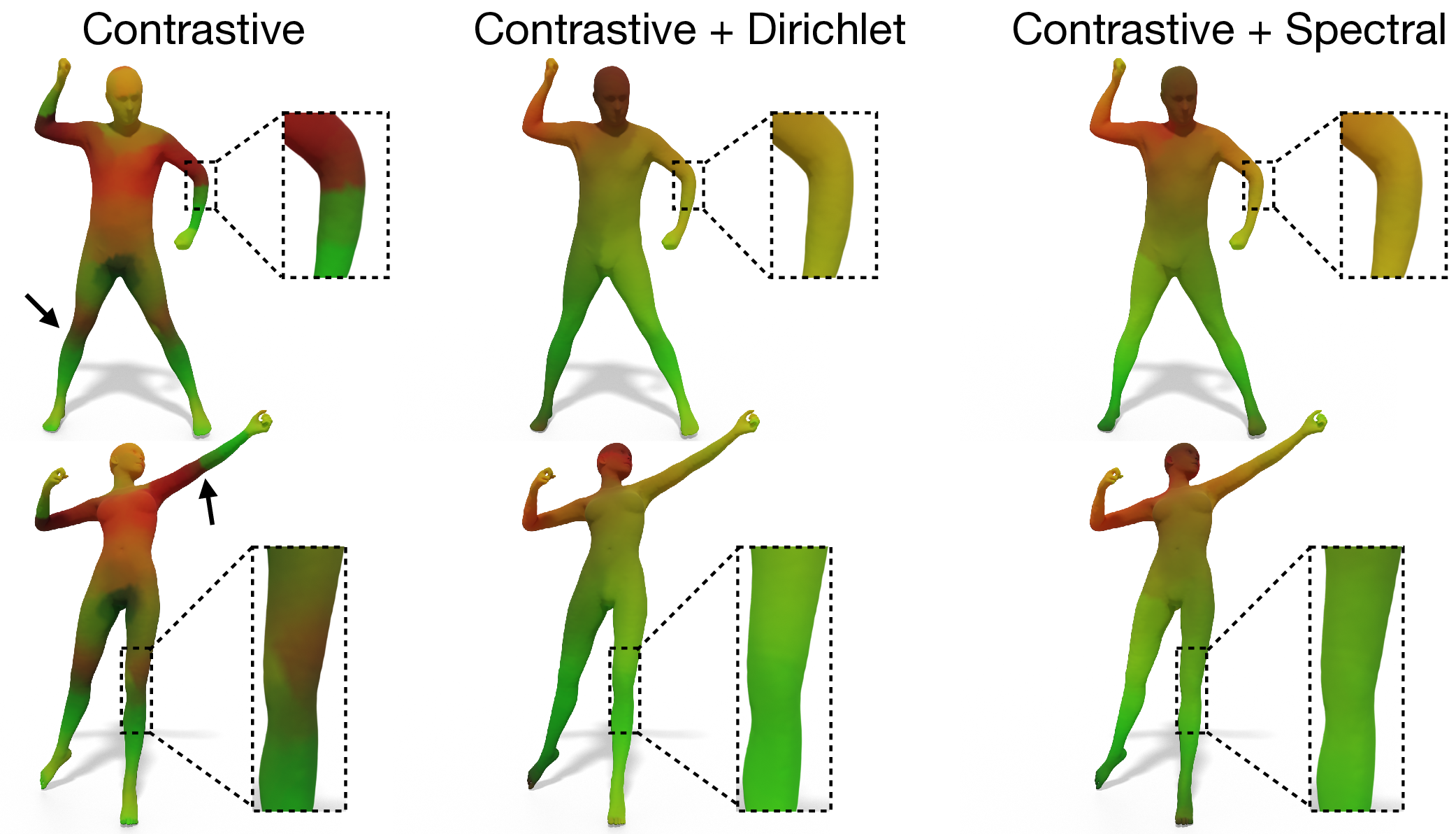
Figure 3: Effect of smoothness regularization on learned local features for a shape pair. 128-dimensional local features are projected to 2D by t-SNE [86] and encoded as colors.

Discussion  To sum up, our SRFeat framework introduces consistency into the contrastive feature learning process through either the Dirichlet energy loss Eq. 7, which regularizes the distribution of features on the points of the domain directly, or the spectral loss Eq. 9, which regularizes correspondences in the reduced spectral basis. Fig. 3 visualizes the effectiveness of smoothness regularization on the learned local features.

We reiterate that SRFeat differs from the currently dominant functional map-based approaches, like GeomFmaps [25] and DPFM [3], for non-rigid shape matching. Firstly, the above works rely on the Laplacian basis and on solving for the optimal functional map matrix at test time, whereas our approach uses nearest-neighbor search directly in the local feature domain. Secondly, since we compute correspondences in the complete basis, foregoing the functional map estimation, our approach can lead to more precise matches and better performance than the above works that only operate in the reduced spectral basis (Sec. 4). Lastly, in our spectral loss Eq. 8 we compute $\mathbf{C}$ directly from a learned soft point-wise map, which avoids the need for solving linear systems inside the network, in contrast to all previous deep functional maps approaches [54, 25, 73, 40, 3], which require differentiating through the matrix inverse, and which can be numerically unstable during training as observed in [73, 25].

3.3 Generalization to 2D Matching

Our SRFeat framework naturally inherits the generality of contrastive learning, although our smoothness regularization losses are firstly formulated in the 3D domain. Indeed, the graph matching problem mentioned in Sec. 3.1 can also benefit from smoothness regularization. Concretely, for the image keypoint matching task [30], each object instance in images is annotated with a set of keypoints for matching. To apply our smoothness regularization, we need to construct a graph for the keypoints of each image object. For this, we adopt the Delaunay triangulation, similar to [31]. The resulting graphs are 2D meshes, and we compute the Laplacian matrix for them in a similar manner to 3D meshes. With this simple adaptation, we can compute the smoothness regularization loss $\mathcal{L}_{\text{s}}$, and combine it with the contrastive loss Eq. 3 to guide the feature learning for graph nodes, as done in Eq. 4. More implementation details are provided in Sec. 4.2.

4 Experiments

We evaluate our SRFeat framework on a wide range of challenging deformable shape matching tasks. First, in Sec. 4.1, we conduct experiments on existing 3D non-rigid shape correspondence benchmarks, including human shape datasets like FAUST [10], SCAPE [1] and SHREC’19 [58], and an animal shape dataset SMAL [100]. Next, in Sec. 4.2, we further investigate the generality of SRFeat in the 2D domain with the PASCAL VOC dataset [30], in the context of keypoint matching across natural images.

4.1 3D Shape Matching

Datasets  The FAUST and SCAPE datasets are widely used for evaluating human shape matching performance. We follow prior works [69, 73, 25, 29] and use the unaligned remeshed versions of the datasets, ensuring that shapes do not share identical mesh connectivity. FAUST contains 100 shapes labeled with ground-truth correspondences, and we use the same training/testing split as the prior works with 80/20 shapes, respectively. SCAPE contains 71 labeled shapes and is split into 51/20 shapes for training/testing.

Due to the nearly saturated performance on FAUST and SCAPE, we also test on SHREC’19 [58], a more challenging human shape matching dataset. SHREC’19 contains 44 labeled shapes with the presence of a partial shape and 430 shape pairs in total. SHREC’19 is used as a test set of generalizability, and we use the training sets of FAUST and SCAPE for network learning.

Finally, we also test on SMAL, a four-legged animal shape dataset with five categories including cats, dogs, cows, horses, and hippos. We use the first three categories as training data with 1,000 shapes per category. The last two categories are only used as testing data with 100 shape pairs for non-isometric matching (i.e., one horse shape and one hippo shape in each testing pair).

Implementation  We use DiffusionNet [78] as the feature extractor $\mathcal{F}_{\Theta}$, which is a generic network for learning features on deformable shapes. The local feature dimension $d$ is set to 128. At training time, for the contrastive loss, we set $\tau=0.07$ in Eq. 1 and randomly sample 1,024 ground-truth correspondences. We use $s(\mathbf{x},\mathbf{y})=\mathbf{x}/\|\mathbf{x}\|_{2}\cdot\mathbf{y}/\|\mathbf{y}\|_{2}$ to make the similarity measurement during training equivalent to the Euclidean distance metric used in proximity search at test time [35]. We performed a simple parameter search to set $\lambda$ in Eq. 4: for the Dirichlet energy loss Eq. 7, we set $\lambda=1$ on all the datasets; for the spectral loss Eq. 9, we set $\lambda=0.1$ on FAUST and $\lambda=10$ on all the other datasets. We use $k=30$ eigenfunctions for the spectral loss, following [25].

Competitors  In Tab. 1, we perform comparisons to several recently proposed approaches for non-rigid shape matching. The first category is axiomatic approaches, including BCICP [69], ZoomOut [59], and Smooth Shells [27]. The second category is unsupervised learning approaches, including SURFMNet [73], UnsupFMNet [40], NeuroMorph [28], and DeepShells [29]. The third category is supervised learning approaches, including FMNet [54], 3D-CODED [36], HSN [93], ACSCNN [53], DPFM[3], and GeomFmaps [25]. Note that for fair comparisons, we reproduced GeomFmaps with DiffusionNet, as done in [78], which shows significantly better performance than the original KPConv-based GeomFmaps [83, 25]. DPFM is also based on DiffusionNet. Post-processing techniques, such as ICP [65], PMF [89], and ZO [59], may be used by the above approaches.

			Train - Test
Method	F	S	F - S	S - F	S19	SMAL
BCICP	6.1	11.0	-	-	-	-
ZoomOut	6.1	7.5	-	-	-	-
SmoothShells	2.5	4.7	-	-	-	-
SURFMNet	15.0	12.0	32.0	32.0	-	-
+ICP	7.4	6.1	19.0	23.0	-	-
UnsupFMNet	10.0	16.0	29.0	22.0	-	-
+PMF	5.7	10.0	12.0	9.3	-	-
NeuroMorph	8.5	29.9	28.5	18.2	-	-
DeepShells	1.7	2.5	5.4	2.7	21.1	12.6
FMNet	11.0	17.0	30.0	33.0	-	-
+PMF	5.9	6.3	11.0	14.0	-	-
3D-CODED	2.5	31.0	31.0	33.0	-	-
HSN	3.3	3.5	25.4	16.7	-	-
ACSCNN	2.7	3.2	8.4	6.0	-	-
DPFM	2.1	2.3	2.7	2.5	6.6	6.3
+ZO	1.9	2.3	2.4	1.9	5.5	5.5
GeomFmaps	2.6	2.9	3.4	3.1	8.5	6.0
+ZO	1.9	2.6	2.6	1.9	7.9	5.6
CL	1.1	1.9	6.1	3.7	10.7	13.7
+ZO	1.9	2.5	2.8	1.9	5.5	5.0
SRFeat-S	1.1	2.2	3.9	2.5	6.1	4.5
+ZO	1.9	2.5	2.6	1.9	4.3	5.3
SRFeat-D	1.1	1.9	4.3	2.2	5.4	3.4
+ZO	1.9	2.5	3.1	1.9	4.6	4.9

Table 1: Evaluation on the FAUST, SCAPE, SHREC’19, and SMAL datasets. The metric is mean geodesic error $\times 100$ on unit-area shapes. The results in gray are obtained by some specific post-processing techniques. The best and second best results without post-refinement are highlighted in each column.

Contrastive learning (CL) is the straightforward baseline of our SRFeat framework, that is, we train the feature extractor with only the contrastive loss $\mathcal{L}_{\text{c}}$ ($\lambda=0$ in Eq. 4). Though being simple, CL is not widely compared in the prior works on non-rigid shape matching, and presents a strong competitive baseline. For our smoothness regularization approach, we denote CL with the Dirichlet energy loss as SRFeat-D, and CL with the spectral loss as SRFeat-S. At test time, we compute correspondences between two input shapes by performing nearest-neighbor search between the learned local features for CL, SRFeat-D, and SRFeat-S.

Results  We use the evaluation metric introduced in [48], i.e., the mean geodesic error on unit-area shapes between the ground-truth and computed correspondences. Tab. 1 shows comparisons on the FAUST, SCAPE, SHREC’19, and SMAL datasets. For the sake of readability, we multiply the results by 100 and mark the results with post-refinement in gray.

On FAUST and SCAPE (Tab. 1-left), our SRFeat shows competitive performance without post-refinement. In the setting of training on FAUST and testing on SCAPE (i.e., F - S), DPFM and GeomFmaps perform better than SRFeat. We ascribe this to the fact that the training set of FAUST contains a relatively small set of poses, which are different from those in SCAPE, and SRFeat is trained to be highly specialized on F with a very low testing error of 1.1, while DPFM and GeomFmaps have 2.1 and 2.6, respectively. Interestingly, the feature matching based methods, i.e., CL, SRFeat-S, and SRFeat-D, achieve saturated performance in the settings of F and S, where post-refinement (i.e., +ZO) hurts the results, indicating that the results below 1.9 on F and 2.5 on S are nearly indistinguishable. This motivates us to focus on the SHREC’19 and SMAL datasets for robustness and generalizability tests, as discussed below. Nevertheless, SRFeat significantly improves CL in the cross dataset settings (F - S and S - F).

On SHREC’19 and SMAL (Tab. 1-right), our SRFeat-D has the best matching performance. We note that these experiments present a very challenging test, which involves non-isometric shape matching and evaluates generalization across datasets (i.e., training on FAUST + SCAPE, testing on SHREC’19) as well as across shape categories (i.e., no category overlap between the training and testing data of SMAL). The experiments show that our SRFeat works well across various challenging testing scenarios and brings consistent improvement to CL.

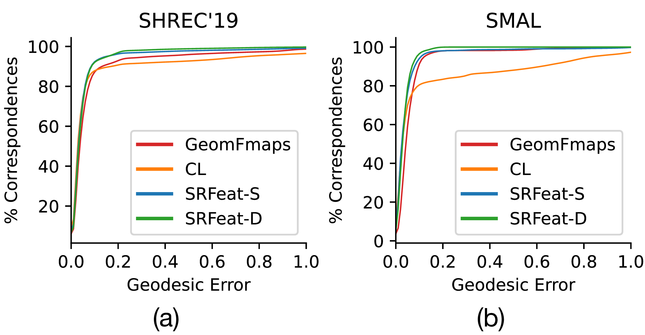
Figure 4: Correspondence quality evaluated on SHREC’19 and SMAL.

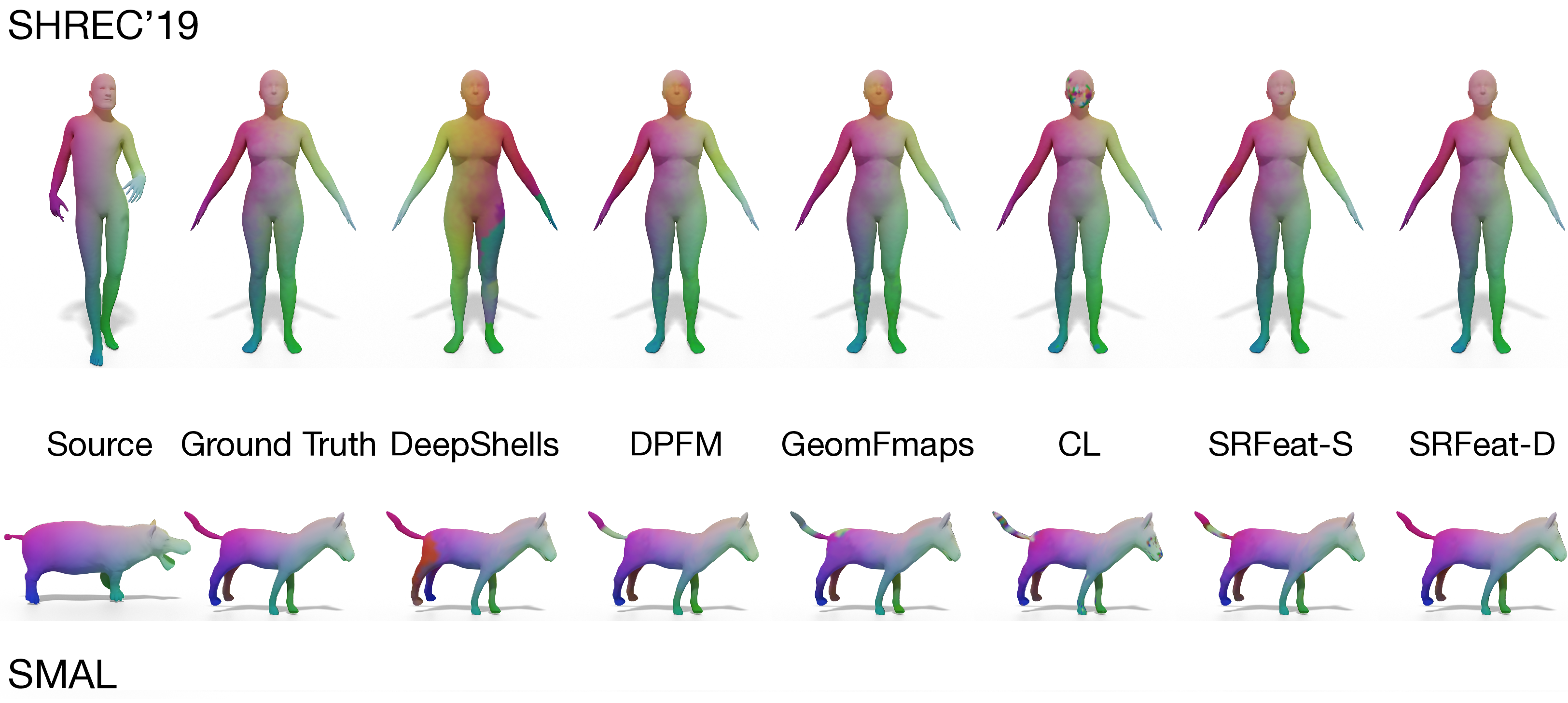
Figure 5: Qualitative results from the SHREC’19 and SMAL datasets without using any post-refinement. Correspondence is visualized by color transfer.

To get a better understanding of the improvement brought by smoothness regularization, in Fig. 4, we plot cumulative curves showing the percentage of correspondences (y-axis) that have geodesic error smaller than a variable threshold (x-axis). The plots show that SRFeat-S and SRFeat-D improve upon CL, and indicate, in particular, that using smoothness regularization in CL helps to significantly reduce correspondences with large errors and thus improves the overall correspondence consistency and quality. In Fig. 5, we show qualitative results without performing any post-refinement, which can better reveal the original correspondence quality produced by each approach. We observe that our SRFeat can produce more accurate correspondences while reducing both local and global artifacts.

Ablation Study  We perform a study w.r.t. the configurations of our approach. First, we have shown the significant contribution of our smoothness regularization losses in Tab. 1 by comparing SRFeat-S and SRFeat-D with the baseline CL (i.e., setting $\lambda=0$ in the training loss Eq. 4).

Next, we test different network architectures for feature extraction. In the above experiments, we use DiffusionNet as the feature extractor, which needs connectivity for feature propagation. In Tab. 2, we test two recent architectures designed for learning on point sets: PointNet++ [67] and SparseConv [18, 17]. We observe that SRFeat-S and SRFeat-D still improve CL noticeably, showing generality across architectures. We find this result to be promising, as it shows that once trained on 3D data with mesh connectivity (used in the smoothness regularization losses), at test time our SRFeat can be applied to non-rigid point sets for local feature extraction and matching without the connectivity information.

Furthermore, we test the robustness of our SRFeat to input noise. We add an increasing amount of Gaussian noise to point positions of shapes in the test set, as shown in Fig. 6 (b), and we do not train or fine-tune the networks on each noise magnitude. We plot the mean geodesic error w.r.t. the noise magnitude in Fig. 6 (a). We observe that SRFeat-S and SRFeat-D consistently improve CL across different noise levels and thus demonstrate the ability to handle moderate amounts of noise.

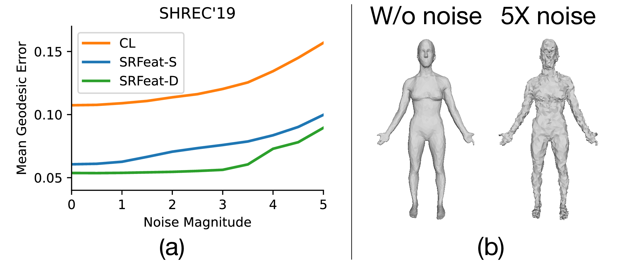
Figure 6: Test with varying noise magnitude on SHREC’19.

Network	CL	SRFeat-S	SRFeat-D
PointNet++	6.2	5.6	5.9
SparseConv	6.9	5.2	3.9

Table 2: Shape matching performance of point-based feature extractors on SMAL (mean geodesic error $\times 100$).

Method	Aero	Bike	Bird	Boat	Bottle	Bus	Car	Cat	Chair	Cow	Table	Dog	Horse	M-Bike	Person	Plant	Sheep	Sofa	Train	TV	Mean
GMN [97]	31.1	46.2	58.2	45.9	70.6	76.5	61.2	61.7	35.5	53.7	58.9	57.5	56.9	49.3	34.1	77.5	57.1	53.6	83.2	88.6	57.9
PCA-GM [91]	40.9	55.0	65.8	47.9	76.9	77.9	63.5	67.4	33.7	66.5	63.6	61.3	58.9	62.8	44.9	77.5	67.4	57.5	86.7	90.9	63.8
DGMC [31]	47.0	65.7	56.8	67.6	86.9	87.7	85.3	72.6	42.9	69.1	84.5	63.8	78.1	55.6	58.4	98.0	68.4	92.2	94.5	85.5	73.0
SRFeat-D	48.4	69.4	57.3	69.8	88.2	86.0	85.8	73.3	42.1	67.7	93.2	67.9	73.2	59.7	58.8	97.1	65.6	95.2	93.8	86.1	73.9
SRFeat-S	49.2	69.1	57.6	68.3	87.7	88.6	85.0	72.9	36.7	64.2	95.1	67.9	76.9	65.0	60.0	96.2	68.6	97.0	93.6	85.7	74.3

Table 3: Keypoint matching in natural images. Hits@1 (%) on the PASCAL VOC dataset with Berkeley keypoint annotations.

4.2 Image Matching

To demonstrate the wide applicability of our smoothness regularization in other modern contrastive feature learning frameworks, we conduct experiments on an existing 2D image keypoint matching benchmark, as discussed in Secs. 3.1 and 3.3.

Dataset  We follow [31] to test on the PASCAL VOC dataset [30] with Berkeley keypoint annotations [12]. The dataset has 6,953 and 1,671 natural images with annotated keypoints for training and testing, respectively. Object instances in the images have varying scale, pose and illumination. The number of keypoints in an object ranges from 1 to 19.

Comparisons  We perform comparisons with recent works GMN [97], PCA-GM [91], and DGMC [31]. DGMC is a recent deep graph matching network that performs node matching between two input graphs based on the node feature similarity, and uses the contrastive loss $\mathcal{L}_{\text{c}}$ in Eq. 3 for training.

Implementation  Our implementation follows DGMC [31]. Specifically, we use SplineCNN [32], a graph neural network, as the feature extractor $\mathcal{F}_{\Theta}$. We apply the Delaunay triangulation to the keypoints in each image for graph construction, which is used in both the graph neural network and our proposed smoothness regularization losses. We augment the contrastive loss $\mathcal{L}_{\text{c}}$ with smoothness regularization, as done in Eq. 4, where we set $\lambda=0.01$ for both the Dirichlet energy loss and the spectral loss. We also use the same training and testing protocols as DGMC.

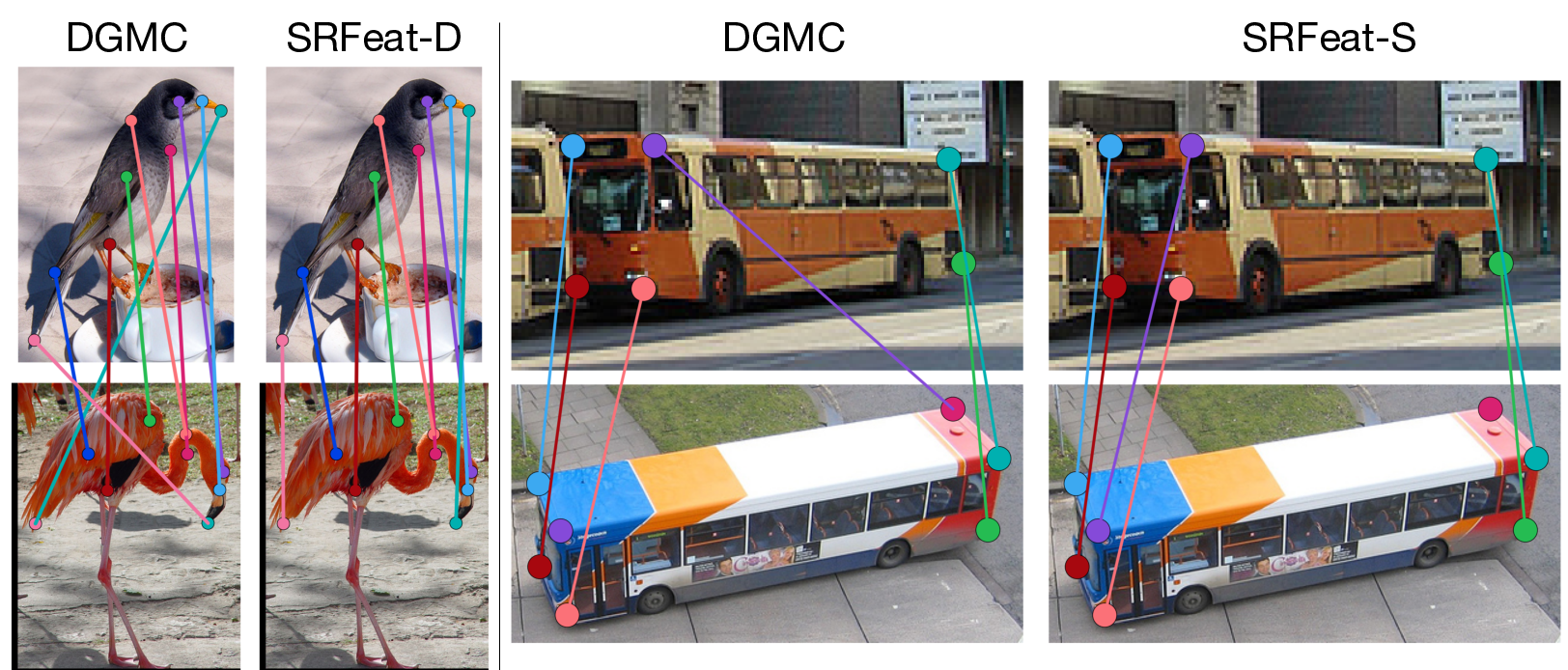
Figure 7: Qualitative results from the PASCAL VOC dataset. Ground-truth corresponding keypoints have the same color.

Results  Tab. 3 presents the performance comparisons on PASCAL VOC. The evaluation metric is Hits@1, measuring the proportion of correctly matched keypoints ranked in the top-1. Fig. 7 further shows qualitative comparisons. We observe that our smoothness regularization brings noticeable improvement over DGMC, which uses contrastive learning only, and SRFeat-S achieves the best performance on this benchmark. We ascribe the slightly better performance of SRFeat-S over SRFeat-D partly to the fact that image objects have very sparse ($\leq 19$) keypoints and may undergo significant geometric distortion and occlusion (Fig. 7). Thus enforcing approximate smoothness and global structure consistency by the spectral loss in a reduced basis can be more beneficial. In contrast, 3D shape matching in Sec. 4.1 is a different application scenario, where dense ($\sim 5,000$) point correspondence is tested. The Dirichlet energy loss encourages the features to vary smoothly on 3D surfaces to better capture the underlying geometry, resulting in more precise dense matching. Nevertheless, the result in Tab. 3 strongly indicates the general applicability of our smoothness-regularized feature learning framework.

5 Conclusion, Limitations & Future Work

In this work, we have presented SRFeat, a generic learning-based framework that combines the local accuracy of contrastive learning with the global consistency of geometric approaches, for robust non-rigid shape correspondence. Through extensive experiments, we show that SRFeat produces discriminative local features that can be robustly matched, resulting in more accurate correspondences. We demonstrate the effectiveness and generality of SRFeat on a suite of benchmarks including 3D non-rigid shape matching and 2D image keypoint matching.

One limitation of our approach is that to compute smoothness regularization we assume the input shapes to be represented as triangle meshes during training, and it might be worth extending our approach to point clouds. For partially overlapped shapes, unlike [3, 45], SRFeat does not have a specific component for predicting overlapping masks used in matching, which might be worth further investigation. Unsupervised learning is another interesting direction to explore. To eschew ground-truth annotations, one possible approach is, like [94], to create synthetic shape pairs via data augmentations. A key challenge would be to systematically study various augmentation strategies for deformable shapes that can lead to informative local feature learning. Finally, further improvements to the matching quality of SRFeat can be brought, e.g., by incorporating a learnable correspondence filtering component [16, 5], in future work.

In this supplementary material, we first include more implementation details in Appendix A. Next, we perform further investigation of our spectral loss in Appendix B. Finally, we present more quantitative and qualitative results in Appendix C.

Appendix A Implementation Details

A.1 3D Shape Matching

We use DiffusionNet [78] as the feature extraction backbone, and its implementation is based on the publicly available codebase released by its authors. The network is composed of four DiffusionNet blocks of width 128. The network takes 3D point positions (i.e., xyz) as input signals and outputs 128-dimensional point-wise features. We set the batch size to 1 and use the ADAM optimizer [49] with an initial learning rate of 0.001. We use servers equipped with NVIDIA A100 and GeForce GTX 1080 GPUs for network training.

In Tab. 4, we show the matching performance w.r.t. $\lambda$ in Eq. (4) on the SHREC’19 and SMAL datasets, resulting in the choice $\lambda=10$ for the spectral loss Eq. (9) and $\lambda=1$ for the Dirichlet energy loss Eq. (7).

In Tab. 5, we show the runtime of shape matching on the SMAL dataset. The statistics were collected on a server with AMD EPYC 7302 CPU, 512GB RAM, and NVIDIA A100 GPU. The columns Feature, FMap, and PMap represent the runtime of feature extraction by DiffusionNet, functional map computation, and point-wise map computation with k-d tree, respectively. We reiterate that the feature matching based methods, i.e., CL, SRFeat-S, and SRFeat-D, do not require functional map computation at test time. Note that the distribution of high dimensional features can affect the nearest neighbor search performance of k-d trees used in the point-wise map computation. Nevertheless, SRFeat-D has the best runtime performance.

A.2 Image Matching

We incorporate our proposed smoothness regularization in DGMC [31] for the 2D image keypoint matching task. Specifically, we build upon the publicly available codebase of DGMC, which is trained with only a contrastive loss, as mentioned in Sec. 3.1 of the main text. In the pre-processing stage, each image is forwarded through a pre-trained VGG16 network, and features of the annotated image keypoints are then extracted on the relu4_2 and relu5_1 feature maps through bilinear interpolation and concatenated together. DGMC adopts SplineCNN, a graph neural network, to extract 256-dimensional node-wise features for matching. Delaunay triangulation is used to construct a graph for the keypoints in each image. To incorporate our smoothness regularization in the training loss, we reuse the triangulation result for the Laplacian matrix construction, which is required in Eq. (6) and (8) of the main text. We set the batch size to 512 and use the ADAM optimizer with a learning rate of 0.001. The network is trained for 15 epochs.

	SHREC’19		SMAL
	SRFeat-S	SRFeat-D	SRFeat-S	SRFeat-D
$\lambda=0.1$	11.2	7.3	14.4	4.8
$\lambda=1$	10.4	5.4	8.6	3.4
$\lambda=10$	6.1	7.2	4.5	5.0
$\lambda=100$	11.1	37.2	6.6	10.7

Table 4: Matching performance w.r.t. $\lambda$ on the SHREC’19 and SMAL datasets (mean geodesic error $\times 100$ on unit-area shapes).

	Feature	FMap	PMap	Total
GeomFmaps	0.0226	0.0437	0.0215	0.0878
CL	0.0227	-	0.0794	0.1021
SRFeat-S	0.0227	-	0.0773	0.1000
SRFeat-D	0.0225	-	0.0419	0.0644

Table 5: Runtime (s) per shape pair averaged on SMAL.

Appendix B Spectral Loss

In Eq. (8) of the main text, we propose to compute a functional map directly from a learned soft point-wise map within the network. In this section, we perform further investigation of Eq. (8) and compare it with the FMReg layer proposed in GeomFmaps [25].

GeomFmaps computes a functional map by treating learned features as probe functions and solving an energy minimization problem in the spectral domain (see Sec. 4.4 of [25]), which is referred as the FMReg layer. This layer, however, needs to solve multiple linear systems within the network, and requires differentiating through the matrix inverse, and thus can be computationally demanding and numerically unstable during training as observed in existing literature [73, 25].

We also compared our proposal based on the definition given in Eq. (8) of the main text, with the FMReg layer introduced in  [25]. For this, we directly replace the FMReg layer in GeomFmaps with our Eq. (8) to compute the functional map $\mathbf{C}$, which is compared to the ground-truth $\mathbf{C}_{\text{gt}}$ as the training loss. The rest of the GeomFmaps network is kept the same.

We remark that GeomFmaps w/ Eq. (8) studied in this additional experiment is a variant of the functional map approaches for shape correspondence, which is different from the feature matching based methods SRFeat-S and SRFeat-D in our main text. Specifically, GeomFmaps w/ Eq. (8) does not use any contrastive learning losses, and requires the Laplacian basis computation and the functional map estimation at test time.

In Tab. 6, we show the matching performance on the SHREC’19 and SMAL datasets. We observe that Eq. (8) improves GeomFmaps on SHREC’19 and has comparable performance with the FMReg layer on SMAL. Note that the performance of our SRFeat-S and SRFeat-D has been reported in Tab. 1 of the main text. We further show the runtime statistics in Tab. 7 and observe that Eq. (8) significantly speeds up the functional map computation by two orders of magnitude (from 0.0437s to 0.0004s) and reduces the overall runtime by more than a half.

	SHREC’19	SMAL
w/ FMReg [25]	8.5	6.0
w/ Eq. (8)	5.8	6.1

Table 6: Matching performance of GeomFmaps [25] with different functional map computation schemes (mean geodesic error $\times 100$ on unit-area shapes).

	Feature	FMap	PMap	Total
w/ FMReg [25]	0.0226	0.0437	0.0215	0.0878
w/ Eq. (8)	0.0226	0.0004	0.0193	0.0423

Table 7: Runtime (s) of GeomFmaps [25] with different functional map computation schemes on SMAL.

Appendix C More Results

In Tab. 8, we show the performance of SRFeat-S-D, which combines CL with the spectral and Dirichlet energy losses. We performed a hyperparameter search to set weights for the spectral and Dirichlet energy losses, resulting in $(0.1,1)$ for SHREC’19, and $(0.1,0.1)$ for SMAL. Observe that this variant slightly outperforms SRFeat-S but is comparable to SRFeat-D, indicating that the Dirichlet energy regularization is sufficient for contrastive learning on 3D shapes. SRFeat-S-D requires more hyperparameter tuning, which may be undesirable in practice.

Method	SHREC’19	SMAL
SRFeat-S	6.1	4.5
SRFeat-D	5.4	3.4
SRFeat-S-D	5.3	3.5

Table 8: Matching performance of SRFeat-S-D (mean geodesic error $\times 100$ on unit-area shapes).

In Fig. 8, we present more qualitative results of non-rigid shape matching on the SHREC’19 and SMAL datasets. We note that the matching results are obtained without performing any post-refinement, which shows the original matching quality of each method. While SRFeat may not be completely free from correspondence outliers, the results show that our smoothness regularization brings noticeable improvement to the matching quality of CL.

In Fig. 9, we also present more qualitative results of the 2D image keypoint matching task on the PASCAL VOC dataset, demonstrating the improvement of SRFeat over DGMC.

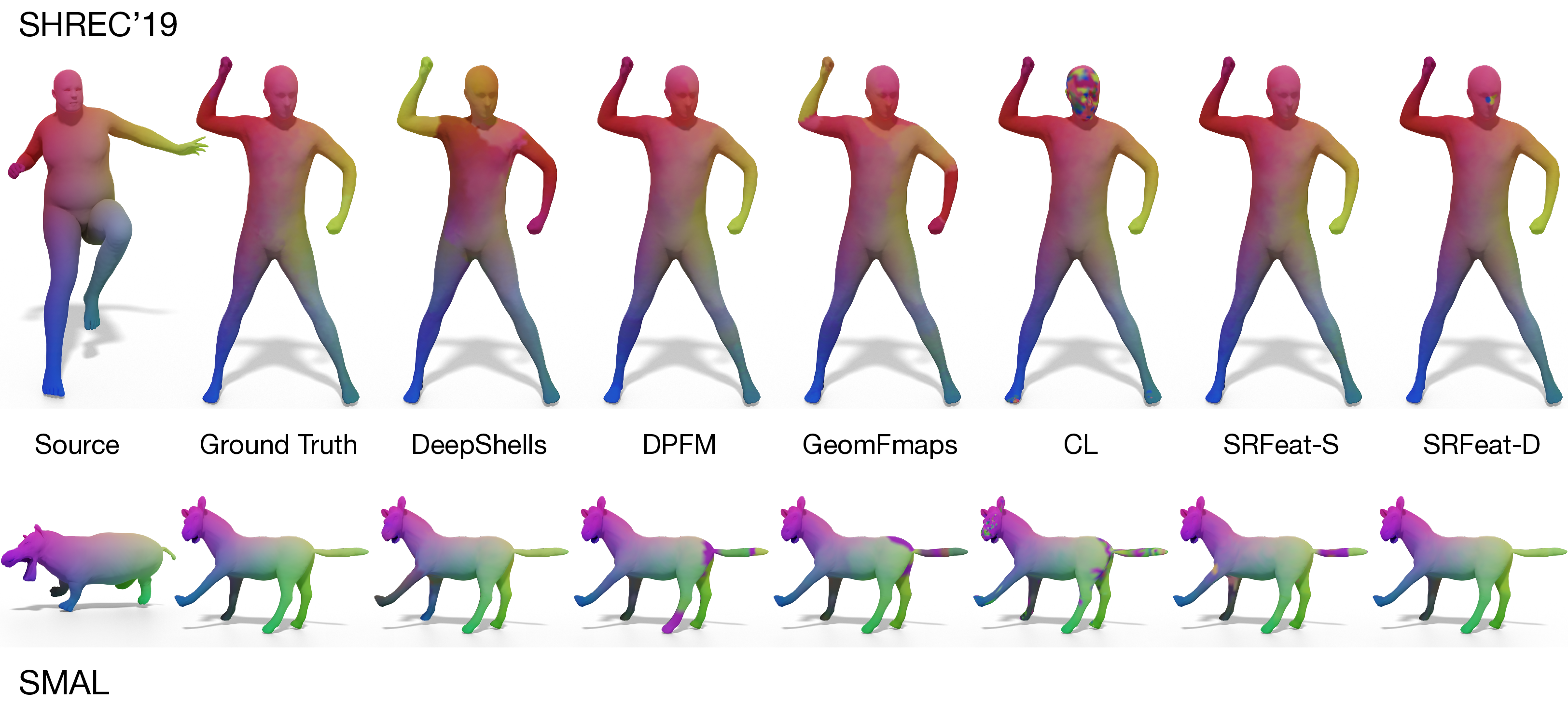
Figure 8: More qualitative results from the SHREC’19 and SMAL datasets without using any post-refinement. Correspondence is visualized by color transfer.

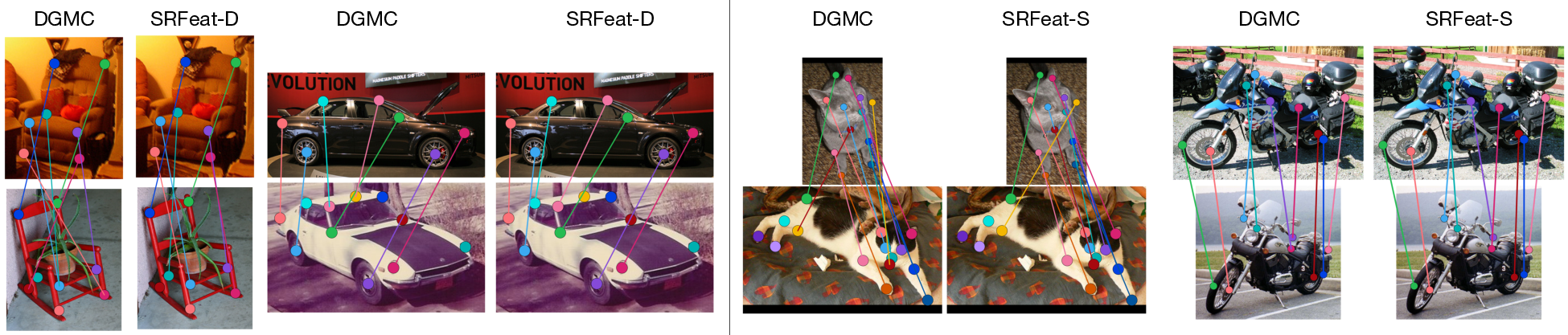
Figure 9: More qualitative results from the PASCAL VOC dataset. Ground-truth corresponding keypoints have the same color.

References

- [1] Dragomir Anguelov, Praveen Srinivasan, Daphne Koller, Sebastian Thrun, Jim Rodgers, and James Davis. SCAPE: shape completion and animation of people. In SIGGRAPH, pages 408–416. 2005.
- [2] Sheng Ao, Qingyong Hu, Bo Yang, Andrew Markham, and Yulan Guo. SpinNet: Learning a general surface descriptor for 3d point cloud registration. In CVPR, 2021.
- [3] Souhaib Attaiki, Gautam Pai, and Maks Ovsjanikov. DPFM: Deep partial functional maps. In 3DV, 2021.
- [4] Mathieu Aubry, Ulrich Schlickewei, and Daniel Cremers. The wave kernel signature: A quantum mechanical approach to shape analysis. In ICCV workshops, pages 1626–1633, 2011.
- [5] Xuyang Bai, Zixin Luo, Lei Zhou, Hongkai Chen, Lei Li, Zeyu Hu, Hongbo Fu, and Chiew-Lan Tai. PointDSC: Robust point cloud registration using deep spatial consistency. In CVPR, 2021.
- [6] Xuyang Bai, Zixin Luo, Lei Zhou, Hongbo Fu, Long Quan, and Chiew-Lan Tai. D3Feat: Joint learning of dense detection and description of 3d local features. In CVPR, 2020.
- [7] Vassileios Balntas, Edward Johns, Lilian Tang, and Krystian Mikolajczyk. Pn-net: Conjoined triple deep network for learning local image descriptors. ArXiv, abs/1601.05030, 2016.
- [8] Vassileios Balntas, Karel Lenc, Andrea Vedaldi, and Krystian Mikolajczyk. Hpatches: A benchmark and evaluation of handcrafted and learned local descriptors. CVPR, pages 3852–3861, 2017.
- [9] Silvia Biasotti, Andrea Cerri, Alex Bronstein, and Michael Bronstein. Recent trends, applications, and perspectives in 3d shape similarity assessment. In CGF, volume 35, pages 87–119, 2016.
- [10] Federica Bogo, Javier Romero, Matthew Loper, and Michael J Black. FAUST: Dataset and evaluation for 3d mesh registration. In CVPR, 2014.
- [11] Davide Boscaini, Jonathan Masci, Emanuele Rodolà, and Michael Bronstein. Learning shape correspondence with anisotropic convolutional neural networks. NeurIPS, 29, 2016.
- [12] Lubomir Bourdev and Jitendra Malik. Poselets: Body part detectors trained using 3d human pose annotations. In ICCV, pages 1365–1372. IEEE, 2009.
- [13] Michael M Bronstein, Joan Bruna, Yann LeCun, Arthur Szlam, and Pierre Vandergheynst. Geometric deep learning: going beyond euclidean data. IEEE Signal Processing Magazine, 34(4):18–42, 2017.
- [14] Oliver Burghard, Alexander Dieckmann, and Reinhard Klein. Embedding shapes with green’s functions for global shape matching. Computers & Graphics, 68:1–10, 2017.
- [15] Ting Chen, Simon Kornblith, Mohammad Norouzi, and Geoffrey Hinton. A simple framework for contrastive learning of visual representations. In ICML, pages 1597–1607, 2020.
- [16] Christopher Choy, Wei Dong, and Vladlen Koltun. Deep global registration. In CVPR, 2020.
- [17] Christopher Choy, JunYoung Gwak, and Silvio Savarese. 4D spatio-temporal convnets: Minkowski convolutional neural networks. In CVPR, 2019.
- [18] Christopher Choy, Jaesik Park, and Vladlen Koltun. Fully convolutional geometric features. In ICCV, 2019.
- [19] Christopher Bongsoo Choy, JunYoung Gwak, Silvio Savarese, and Manmohan Chandraker. Universal correspondence network. In NeurIPS, 2016.
- [20] Jiequan Cui, Zhisheng Zhong, Shu Liu, Bei Yu, and Jiaya Jia. Parametric contrastive learning. In ICCV, 2021.
- [21] Angela Dai, Angel X. Chang, Manolis Savva, Maciej Halber, Thomas Funkhouser, and Matthias Nießner. ScanNet: Richly-annotated 3d reconstructions of indoor scenes. In CVPR, 2017.
- [22] Bailin Deng, Yuxin Yao, Roberto M Dyke, and Juyong Zhang. A survey of non-rigid 3d registration. In CGF, volume 41, pages 559–589, 2022.
- [23] Haowen Deng, Tolga Birdal, and Slobodan Ilic. PPFNet: Global context aware local features for robust 3d point matching. In CVPR, 2018.
- [24] Huong Quynh Dinh, Anthony Yezzi, and Greg Turk. Texture transfer during shape transformation. ACM TOG, 24(2):289–310, 2005.
- [25] Nicolas Donati, Abhishek Sharma, and Maks Ovsjanikov. Deep geometric functional maps: Robust feature learning for shape correspondence. In CVPR, 2020.
- [26] Bi’an Du, Xiang Gao, Wei Hu, and Xin Li. Self-contrastive learning with hard negative sampling for self-supervised point cloud learning. In ACM MM, pages 3133–3142, 2021.
- [27] Marvin Eisenberger, Zorah Lahner, and Daniel Cremers. Smooth shells: Multi-scale shape registration with functional maps. In CVPR, pages 12265–12274, 2020.
- [28] Marvin Eisenberger, David Novotny, Gael Kerchenbaum, Patrick Labatut, Natalia Neverova, Daniel Cremers, and Andrea Vedaldi. NeuroMorph: Unsupervised shape interpolation and correspondence in one go. In CVPR, 2021.
- [29] Marvin Eisenberger, Aysim Toker, Laura Leal-Taixé, and Daniel Cremers. Deep Shells: Unsupervised shape correspondence with optimal transport. arXiv, 2020.
- [30] Mark Everingham, Luc Van Gool, Christopher KI Williams, John Winn, and Andrew Zisserman. The PASCAL visual object classes (VOC) challenge. IJCV, 88(2):303–338, 2010.
- [31] M. Fey, J. E. Lenssen, C. Morris, J. Masci, and N. M. Kriege. Deep graph matching consensus. In ICLR, 2020.
- [32] Matthias Fey, Jan Eric Lenssen, Frank Weichert, and Heinrich Müller. SplineCNN: Fast geometric deep learning with continuous b-spline kernels. In CVPR, June 2018.
- [33] Andrea Frome, Daniel Huber, Ravi Kolluri, Thomas Bülow, and Jitendra Malik. Recognizing objects in range data using regional point descriptors. In ECCV, 2004.
- [34] Zan Gojcic, Caifa Zhou, Jan D. Wegner, and Andreas Wieser. The perfect match: 3D point cloud matching with smoothed densities. In CVPR, 2019.
- [35] Jean-Bastien Grill, Florian Strub, Florent Altché, Corentin Tallec, Pierre H Richemond, Elena Buchatskaya, Carl Doersch, Bernardo Avila Pires, Zhaohan Daniel Guo, Mohammad Gheshlaghi Azar, et al. Bootstrap your own latent: A new approach to self-supervised learning. arXiv, 2020.
- [36] Thibault Groueix, Matthew Fisher, Vladimir G. Kim, Bryan C. Russell, and Mathieu Aubry. 3D-CODED: 3d correspondences by deep deformation. In ECCV, 2018.
- [37] Yulan Guo, Mohammed Bennamoun, Ferdous Sohel, Min Lu, Jianwei Wan, and Ngai Ming Kwok. A comprehensive performance evaluation of 3d local feature descriptors. IJCV, 116(1), 2016.
- [38] Yulan Guo, Hanyun Wang, Qingyong Hu, Hao Liu, Li Liu, and Mohammed Bennamoun. Deep learning for 3d point clouds: A survey. IEEE TPAMI, 2020.
- [39] Raia Hadsell, Sumit Chopra, and Yann LeCun. Dimensionality reduction by learning an invariant mapping. In CVPR, 2006.
- [40] Oshri Halimi, Or Litany, Emanuele Rodola, Alex M. Bronstein, and Ron Kimmel. Unsupervised learning of dense shape correspondence. In CVPR, 2019.
- [41] Kaiming He, Haoqi Fan, Yuxin Wu, Saining Xie, and Ross Girshick. Momentum contrast for unsupervised visual representation learning. In CVPR, pages 9729–9738, 2020.
- [42] Ji Hou, Benjamin Graham, Matthias Niessner, and Saining Xie. Exploring data-efficient 3d scene understanding with contrastive scene contexts. In CVPR, 2021.
- [43] Qixing Huang, Fan Wang, and Leonidas Guibas. Functional map networks for analyzing and exploring large shape collections. ACM TOG, 33(4):1–11, 2014.
- [44] Ruqi Huang and Maks Ovsjanikov. Adjoint map representation for shape analysis and matching. In CGF, volume 36, pages 151–163. Wiley Online Library, 2017.
- [45] Shengyu Huang, Zan Gojcic, Mikhail Usvyatsov, Andreas Wieser, and Konrad Schindler. PREDATOR: Registration of 3d point clouds with low overlap. arXiv, 2020.
- [46] Siyuan Huang, Yichen Xie, Song-Chun Zhu, and Yixin Zhu. Spatio-temporal self-supervised representation learning for 3d point clouds. In ICCV, pages 6535–6545, 2021.
- [47] A. E. Johnson and M. Hebert. Using spin images for efficient object recognition in cluttered 3d scenes. IEEE TPAMI, 21(5), 1999.
- [48] Vladimir G Kim, Yaron Lipman, and Thomas Funkhouser. Blended intrinsic maps. ACM TOG, 30(4):1–12, 2011.
- [49] Diederik P. Kingma and Jimmy Ba. Adam: A method for stochastic optimization. In ICLR, 2015.
- [50] Artiom Kovnatsky, Michael M Bronstein, Alexander M Bronstein, Klaus Glashoff, and Ron Kimmel. Coupled quasi-harmonic bases. In CGF, volume 32, pages 439–448, 2013.
- [51] Karel Lenc and Andrea Vedaldi. Large scale evaluation of local image feature detectors on homography datasets. ArXiv, abs/1807.07939, 2018.
- [52] Lei Li, Siyu Zhu, Hongbo Fu, Ping Tan, and Chiew-Lan Tai. End-to-end learning local multi-view descriptors for 3D point clouds. In CVPR, 2020.
- [53] Qinsong Li, Shengjun Liu, Ling Hu, and Xinru Liu. Shape correspondence using anisotropic Chebyshev spectral cnns. In CVPR, June 2020.
- [54] Or Litany, Tal Remez, Emanuele Rodola, Alex Bronstein, and Michael Bronstein. Deep functional maps: Structured prediction for dense shape correspondence. In ICCV, 2017.
- [55] David G. Lowe. Distinctive image features from scale-invariant keypoints. IJCV, 60(2), 2004.
- [56] Jiayi Ma, Xingyu Jiang, Aoxiang Fan, Junjun Jiang, and Junchi Yan. Image matching from handcrafted to deep features: A survey. IJCV, 129(1):23–79, Aug. 2020.
- [57] Jonathan Masci, Davide Boscaini, Michael M. Bronstein, and Pierre Vandergheynst. Geodesic convolutional neural networks on riemannian manifolds. In ICCV Workshops, 2015.
- [58] Simone Melzi, Riccardo Marin, Emanuele Rodolà, Umberto Castellani, Jing Ren, Adrien Poulenard, Peter Wonka, and Maks Ovsjanikov. Matching humans with different connectivity. In 3DOR, pages 121–128, 2019.
- [59] Simone Melzi, Jing Ren, Emanuele Rodolà, Abhishek Sharma, Peter Wonka, and Maks Ovsjanikov. ZoomOut: Spectral upsampling for efficient shape correspondence. ACM TOG, 38(6), Nov. 2019.
- [60] Krystian Mikolajczyk and Cordelia Schmid. An affine invariant interest point detector. In ECCV, pages 128–142. 2002.
- [61] Thomas W. Mitchel, Vladimir G. Kim, and Michael Kazhdan. Field convolutions for surface cnns. In ICCV, 2021.
- [62] Dorian Nogneng and Maks Ovsjanikov. Informative descriptor preservation via commutativity for shape matching. In CGF, volume 36, pages 259–267. Wiley Online Library, 2017.
- [63] Hyeonwoo Noh, Andre F. de Araújo, Jack Sim, Tobias Weyand, and Bohyung Han. Large-scale image retrieval with attentive deep local features. ICCV, pages 3476–3485, 2017.
- [64] Aaron van den Oord, Yazhe Li, and Oriol Vinyals. Representation learning with contrastive predictive coding. arXiv, 2018.
- [65] Maks Ovsjanikov, Mirela Ben-Chen, Justin Solomon, Adrian Butscher, and Leonidas Guibas. Functional maps: a flexible representation of maps between shapes. ACM TOG, 31(4):1–11, 2012.
- [66] Ulrich Pinkall and Konrad Polthier. Computing discrete minimal surfaces and their conjugates. Experimental mathematics, 2(1):15–36, 1993.
- [67] Charles Ruizhongtai Qi, Li Yi, Hao Su, and Leonidas J Guibas. PointNet++: Deep hierarchical feature learning on point sets in a metric space. NeurIPS, 30, 2017.
- [68] Yongming Rao, Benlin Liu, Yi Wei, Jiwen Lu, Cho-Jui Hsieh, and Jie Zhou. RandomRooms: Unsupervised pre-training from synthetic shapes and randomized layouts for 3d object detection. In ICCV, pages 3283–3292, 2021.
- [69] Jing Ren, Adrien Poulenard, Peter Wonka, and Maks Ovsjanikov. Continuous and orientation-preserving correspondences via functional maps. ACM TOG, 37(6):1–16, 2018.
- [70] I. Rocco, M. Cimpoi, R. Arandjelović, A. Torii, T. Pajdla, and J. Sivic. Neighbourhood consensus networks. In NeurIPS, 2018.
- [71] Emanuele Rodolà, Luca Cosmo, Michael M Bronstein, Andrea Torsello, and Daniel Cremers. Partial functional correspondence. In CGF, volume 36, pages 222–236, 2017.
- [72] Reihaneh Rostami, Fereshteh S Bashiri, Behrouz Rostami, and Zeyun Yu. A survey on data-driven 3d shape descriptors. In CGF, volume 38, pages 356–393, 2019.
- [73] Jean-Michel Roufosse, Abhishek Sharma, and Maks Ovsjanikov. Unsupervised deep learning for structured shape matching. In ICCV, 2019.
- [74] R. B. Rusu, N. Blodow, and M. Beetz. Fast point feature histograms (fpfh) for 3d registration. In ICRA, 2009.
- [75] R. B. Rusu, N. Blodow, Z. C. Marton, and M. Beetz. Aligning point cloud views using persistent feature histograms. In IROS, 2008.
- [76] Samuele Salti, Federico Tombari, and Luigi di Stefano. SHOT: Unique signatures of histograms for surface and texture description. CVIU, 125, 2014.
- [77] Paul-Edouard Sarlin, Daniel DeTone, Tomasz Malisiewicz, and Andrew Rabinovich. SuperGlue: Learning feature matching with graph neural networks. In CVPR, 2020.
- [78] Nicholas Sharp, Souhaib Attaiki, Keenan Crane, and Maks Ovsjanikov. DiffusionNet: discretization agnostic learning on surfaces. ACM TOG, 41(3), 2022.
- [79] Edgar Simo-Serra, Eduard Trulls, Luis Ferraz, Iasonas Kokkinos, Pascal Fua, and Francesc Moreno-Noguer. Discriminative learning of deep convolutional feature point descriptors. In ICCV, Dec. 2015.
- [80] Karen Simonyan, Andrea Vedaldi, and Andrew Zisserman. Learning local feature descriptors using convex optimisation. IEEE TPAMI, 36(8):1573–1585, Aug. 2014.
- [81] Jian Sun, Maks Ovsjanikov, and Leonidas Guibas. A concise and provably informative multi-scale signature based on heat diffusion. In CGF, volume 28, pages 1383–1392, 2009.
- [82] Gary KL Tam, Zhi-Quan Cheng, Yu-Kun Lai, Frank C Langbein, Yonghuai Liu, David Marshall, Ralph R Martin, Xian-Fang Sun, and Paul L Rosin. Registration of 3d point clouds and meshes: A survey from rigid to nonrigid. IEEE TVCG, 19(7), 2012.
- [83] Hugues Thomas, Charles R. Qi, Jean-Emmanuel Deschaud, Beatriz Marcotegui, Francois Goulette, and Leonidas J. Guibas. KPConv: Flexible and deformable convolution for point clouds. In ICCV, 2019.
- [84] Tinne Tuytelaars and Krystian Mikolajczyk. Local invariant feature detectors: A survey. Foundations and Trends® in Computer Graphics and Vision, 3(3):177–280, 2007.
- [85] Bruno Vallet and Bruno Lévy. Spectral geometry processing with manifold harmonics. In CGF, volume 27, pages 251–260, 2008.
- [86] Laurens Van der Maaten and Geoffrey Hinton. Visualizing data using t-sne. Journal of machine learning research, 9(11), 2008.
- [87] Oliver Van Kaick, Hao Zhang, Ghassan Hamarneh, and Daniel Cohen-Or. A survey on shape correspondence. In CGF, volume 30, pages 1681–1707. Wiley Online Library, 2011.
- [88] Daniel Ponsa Vassileios Balntas, Edgar Riba and Krystian Mikolajczyk. Learning local feature descriptors with triplets and shallow convolutional neural networks. In BMVC, pages 119.1–119.11, September 2016.
- [89] Matthias Vestner, Roee Litman, Emanuele Rodola, Alex Bronstein, and Daniel Cremers. Product manifold filter: Non-rigid shape correspondence via kernel density estimation in the product space. In CVPR, pages 3327–3336, 2017.
- [90] Peng-Shuai Wang, Yu-Qi Yang, Qian-Fang Zou, Zhirong Wu, Yang Liu, and Xin Tong. Unsupervised 3d learning for shape analysis via multiresolution instance discrimination. In AAAI, 2021.
- [91] Runzhong Wang, Junchi Yan, and Xiaokang Yang. Learning combinatorial embedding networks for deep graph matching. In CVPR, pages 3056–3065, 2019.
- [92] Yue Wang and Justin M. Solomon. Deep closest point: Learning representations for point cloud registration. In ICCV, 2019.
- [93] Ruben Wiersma, Elmar Eisemann, and Klaus Hildebrandt. CNNs on surfaces using rotation-equivariant features. ACM TOG, 39(4):92–1, 2020.
- [94] Saining Xie, Jiatao Gu, Demi Guo, Charles R Qi, Leonidas Guibas, and Or Litany. PointContrast: Unsupervised pre-training for 3d point cloud understanding. In ECCV, 2020.
- [95] Zi Jian Yew and Gim Hee Lee. RPM-Net: Robust point matching using learned features. In CVPR, 2020.
- [96] Kwang Moo Yi, Eduard Trulls, Vincent Lepetit, and Pascal Fua. LIFT: Learned invariant feature transform. In ECCV, pages 467–483. 2016.
- [97] Andrei Zanfir and Cristian Sminchisescu. Deep learning of graph matching. In CVPR, 2018.
- [98] Andy Zeng, Shuran Song, Matthias Niessner, Matthew Fisher, Jianxiong Xiao, and Thomas Funkhouser. 3DMatch: Learning local geometric descriptors from rgb-d reconstructions. In CVPR, 2017.
- [99] Qian-Yi Zhou, Jaesik Park, and Vladlen Koltun. Fast global registration. In ECCV, 2016.
- [100] Silvia Zuffi, Angjoo Kanazawa, David W. Jacobs, and Michael J. Black. 3D Menagerie: Modeling the 3d shape and pose of animals. In CVPR, 2017.