Nonparametric Estimation via Mixed Gradients

Abstract

Traditional nonparametric estimation methods often lead to a slow convergence rate in large dimensions and require unrealistically enormous sizes of datasets for reliable conclusions. We develop an approach based on mixed gradients, either observed or estimated, to effectively estimate the function at near-parametric convergence rates. The novel approach and computational algorithm could lead to methods useful to practitioners in many areas of science and engineering. Our theoretical results reveal a behavior universal to this class of nonparametric estimation problems. We explore a general setting involving tensor product spaces and build upon the smoothing spline analysis of variance (SS-ANOVA) framework. For $d$-dimensional models under full interaction, the optimal rates with gradient information on $p$ covariates are identical to those for the $(d-p)$-interaction models without gradients and, therefore, the models are immune to the “curse of interaction”. For additive models, the optimal rates using gradient information are root-$n$, thus achieving the “parametric rate”. We demonstrate aspects of the theoretical results through synthetic and real data applications.

Key Words: Gradient; Interaction; Reproducing kernel Hilbert space; Smoothing spline ANOVA; Time series.

1 Introduction

Gradient information for complex systems arises in many areas of science and engineering. Economists estimate cost functions, where data on factor demands and costs are collected together. By Shephard’s Lemma, the demand functions are the first-order partial derivatives of the cost function (Hall and Yatchew, 2007). In actuarial science, demography gives mortality force data, which, together with samples from the survival distribution, yield gradients for the survival distribution function (Frees and Valdez, 1998). In the stochastic simulation, gradient estimation has been studied for a large class of problems (Glasserman, 2013). In discrete event simulation, the gradient can be estimated with a negligible computational burden compared to the effort for obtaining a new response (Chen et al., 2013). In meteorology, wind speed and direction are gradient functions of the barometric pressure, and they are measured over broad geographic regions (Breckling, 2012). In dynamical and time series applications, gradient information can be observed or estimated, such as in biological and infectious disease modeling (Dai and Li, 2021). In traffic engineering, real-time motion sensors can record velocity in addition to positions (Solak et al., 2002).

This paper focuses on nonparametric function estimation under smoothness constraints. Rates of convergence often limit the applications of traditional nonparametric estimation methods in high-dimensional settings, where the number of covariates is large (Stone, 1980, 1982). A considerable amount of research effort has been devoted to countering this curse of dimensionality. The additive model is a popular choice (Stone, 1985; Hastie and Tibshirani, 1990). An additive model assumes the high-dimensional function to be a sum of one-dimensional functions and drops interactions among covariates in order to reduce the variability of an estimator. Stone (1985) showed that the optimal convergence rate for additive models is the same as that for univariate nonparametric estimation problems. Thus, the additive models effectively mitigate the curse of dimensionality. Additive models, however, could be too restrictive and lead to wrong conclusions in applications where interactions among the covariates may be present. As a more flexible alternative, smoothing spline analysis of variance (SS-ANOVA) models, the analogs of parametric ANOVA models, have attracted lots of attention (Wahba et al., 1995; Huang, 1998; Lin and Zhang, 2006; Zhu et al., 2014). In particular, SS-ANOVA models include additive models as special cases. Lin (2000) proved that when the interactions among covariates are in tensor product spaces, the optimal rates of convergence for SS-ANOVA models exponentially depend on the order of interaction. Thus, when SS-ANOVA models are used in problems that involve high-order interactions, it leads to requiring unrealistically enormous sizes of datasets for reliable conclusions. We call this phenomenon curse of interaction.

We develop a new approach based on mixed gradients to effectively compromise the curse of interaction. Let $\{({\bf{t}}_{i}^{(0)},y_{i}^{(0)}):i=1,\ldots,n\}$ be the function data that follow a regression model,

$$Y^{(0)}=f_{0}({\bf{t}}^{(0)})+\epsilon^{(0)}.$$ (1)

Here $\epsilon^{(0)}\in\mathbb{R}$ is a random error, $f_{0}:\mathcal{X}^{d}\mapsto\mathbb{R}$ is a function of $d$ covariates ${\bf{t}}=(t_{1},\ldots,t_{d})$, and ${\bf{t}}^{(0)}\in\mathcal{X}^{d}\equiv[0,1]^{d}$ is the design point. Write $\partial f_{0}({\bf{t}})/\partial t_{j}$ as the $j$th partial derivative of $f_{0}({\bf{t}})$. Let $\{({\bf{t}}_{i}^{(j)},y_{i}^{(j)}):i=1,\ldots,n;j=1,\ldots,p\}$ be the mixed gradients that follow a regression model,

$$Y^{(j)}=\frac{\partial f_{0}({\bf{t}}^{(j)})}{\partial t_{j}}+\epsilon^{(j)},\quad j=1,\ldots,p.$$ (2)

Here $\epsilon^{(j)}$s are random errors, and ${\bf{t}}^{(j)}$s are the design points in $\mathcal{X}^{d}$. We allow $Y^{(j)}$ to be directly observable or estimated from function data. The $p\in\{1,\ldots,d\}$ denotes the number of gradient types. Without loss of generality, we focus on the first $p$ covariates in model (2). In particular, when $p=d$, model (2) gives the full gradient data. We allow for a relaxed error structure for both function and gradient data. Specifically, we assume the random errors $\epsilon^{(0)}$ and $\epsilon^{(j)}$s in models (1) and (2) to satisfy,

$$\mathbb{E}[\epsilon_{i}^{(j)}]=o(n^{-1/2}),\ \ \text{Var}[\epsilon_{i}^{(j)}]=\sigma_{j}^{2}<\infty,$$ (3)

$$\text{Cov}[\epsilon_{i}^{(j)},\epsilon_{i^{\prime}}^{(j^{\prime})}]=O\left(|i-i^{\prime}|^{-\Upsilon}\right)\ \ \text{for some }\Upsilon>1,$$

where $i\neq i^{\prime}$ and $j,j^{\prime}=0,1,\ldots,p$. We assume the short-range correlation in (3) with some $\Upsilon>1$. This is common in practice because gradient data are usually estimated using local function data via, for example, the finite-difference methods. The random errors in (3) can be uncentered and correlated, which are typical for estimated gradient data, and include the setting of i.i.d. errors as a special case (Hall and Yatchew, 2007).

The SS-ANOVA model (Wahba et al., 1995) amounts to the assumption that

$$f_{0}({\bf{t}})=\mbox{constant}+\sum_{j=1}^{d}f_{0j}(t_{j})+\cdots+\sum_{1\leq j_{1}<j_{2}<\cdots<j_{r}\leq d}f_{0j_{1}j_{2}\cdots j_{r}}(t_{j_{1}},t_{j_{2}},\ldots,t_{j_{r}}),$$ (4)

where the component functions include main effects $f_{0j}$s, two-way interactions $f_{0j_{1}j_{2}}$s, and so on. Component functions are modeled nonparametrically, and we assume that they reside in certain reproducing kernel Hilbert spaces (RKHS, Wahba, 1990). The series on the right-hand side of (4) is truncated to some order $r$ of interactions to enhance interpretability. We call $f_{0}(t)$ as full or truncated interaction SS-ANOVA model if $r=d$ or $1\leq r<d$, respectively. The SS-ANOVA model (4) can be identified with space,

$$\mathcal{H} =\{1\}\oplus\sum_{j=1}^{d}\mathcal{H}^{j}\oplus\cdots\oplus\sum_{1\leq j_{1}<j_{2}<\cdots<j_{r}\leq d}\left[\mathcal{H}^{j_{1}}\otimes\mathcal{H}^{j_{2}}\otimes\cdots\otimes\mathcal{H}^{j_{r}}\right].$$ (5)

The components of the SS-ANOVA model in (4) are in the mutually orthogonal subspaces of $\mathcal{H}$ in (5). The additive model can be viewed as a special case of the SS-ANOVA model (4) by taking $r=1$. We assume that all component functions come from a common RKHS $(\mathcal{H}_{1},\|\cdot\|_{\mathcal{H}_{1}})$ given by $\mathcal{H}^{j}\equiv\mathcal{H}_{1}$ for $j=1,\ldots,d$. Obviously the linear model is a special example of (4) by taking $r=1$ and letting $\mathcal{H}_{1}$ be the collection of all univariate linear functions defined over $\mathcal{X}$. Another canonical example of $\mathcal{H}_{1}$ is the $m$th order Sobolev space $\mathcal{W}_{2}^{m}(\mathcal{X})$; see, e.g., Wahba (1990) for further examples.

We study the possibility of near-parametric rates in the general setting of SS-ANOVA models. Suppose the eigenvalues of the kernel function decay polynomially, i.e., its $\nu$th largest eigenvalue is of the order $\nu^{-2m}$. Our results show that the minimax optimal rates for estimating $f_{0}$ under the full interaction (i.e., $r=d$) are

$$\mathcal{R}(n,d,r,p)=\begin{cases}\left[n(\log n)^{1+p-d}\right]^{-\frac{2m}{2m+1}},&\mbox{ if }0\leq p<d,\\ n^{-\frac{2md}{(2m+1)d-2}}\mathbbm{1}_{d\geq 3}+n^{-1}(\log n)^{d-1}\mathbbm{1}_{d<3},&\mbox{ if }p=d.\end{cases}$$ (6)

The rates in (6) exhibit an interesting two-regime dichotomy of $0\leq p<d$ and $p=d$. When $0\leq p<d$, the rate given by (6) happens to be the minimax optimal rate for estimating a $(d-p)$-interaction model without gradient information (Lin, 2000). For instance, when $p=d-1$, the rate given by (6) becomes $n^{-2m/(2m+1)}$, which is identical to the optimal rate for estimating additive models without gradient information (Stone, 1985). Hence, SS-ANOVA models are immune to the curse of interaction by using mixed gradients. On the other hand, when $p=d\geq 3$, the rate in (6) becomes

$$\mathcal{R}(n,d,r,p)=n^{-\frac{2md}{(2m+1)d-2}}.$$

This rate converges faster than the optimal rate for additive models $n^{-2m/(2m+1)}$. When $p=d=2$, the rate in (6) is $\mathcal{R}(n,d,r,p)=n^{-1}\log n$. If $p=d=1$, the rate in (6) is the same as the parametric convergence rate, $\mathcal{R}(n,d,r,p)=n^{-1}$. It is also worth pointing out that if $f_{0}$ has truncated interaction (i.e., $r<d$), the rates are also accelerated based on mixed gradients, which will be discussed in Section 3. In particular, the rate for additive models (i.e., $r=1$) under $p=d$ coincides with the parametric rate, $\mathcal{R}(n,d,r,p)=n^{-1}$. A similar phenomenon on the accelerated rates has been observed earlier given higher-order derivatives (Hall and Yatchew, 2007, 2010). Our results suggest that such a phenomenon holds with first-order derivatives (i.e., mixed gradients) and applies to a general setting involving tensor product spaces for mitigating the curse of interaction.

1.1 Our contributions

We develop an approach and computational algorithm to incorporate mixed gradients and lead to methods useful to practitioners in many areas of science and engineering. We obtain a new theory that reveals a behavior universal to this class of nonparametric estimation problems. Our proposal and theoretical results considerably differ from the existing works in multiple ways, which are summarized as follows.

First, our results broaden the i.i.d. error structure by allowing the random errors in function data and gradient data to be biased and correlated. This relaxed assumption is in line with applications when the gradient data are estimated (Chen et al., 2013).

Second, we develop a new approach and computational algorithm in RKHS that can easily incorporate gradient information. The proposed estimator also enjoys interpretability by providing a direct description of interactions. We also find that mixed gradients can reduce interactions in terms of the minimax convergence rates.

Finally, we obtain a sharper theory on the estimation with mixed gradients. We show that when $p=d-1$, the optimal rate for estimating $d$-dimensional SS-ANOVA models under full interaction is $n^{-2m/(2m+1)}$, which is independent of the interaction order $r$. Hence the SS-ANOVA models are immune to the curse of interaction via using gradients. In contrast, Hall and Yatchew (2007) showed that when $p=d-1$, the convergence rate for estimating $d$-dimensional functions is $n^{-2m/(2m+d-1)}$, which has the curse of dimensionality in $d$. Therefore, our results show that mixed gradients are useful for the scalability of nonparametric estimation in high dimensions, particularly when using the SS-ANOVA models.

The rest sections are organized as follows. We first provide background in Section 2, and show main results in Section 3. Section 4 presents synthetic and real data examples. Section 5 discusses related works. We provide conclusion in Section 6. The results under other types of designs and their proofs, together with additional numerical examples, are relegated to the Appendix.

2 Background

We begin with a motivating example with mixed gradients. Then we briefly review basic facts about RKHS for the setting of our interest.

2.1 Motivating example

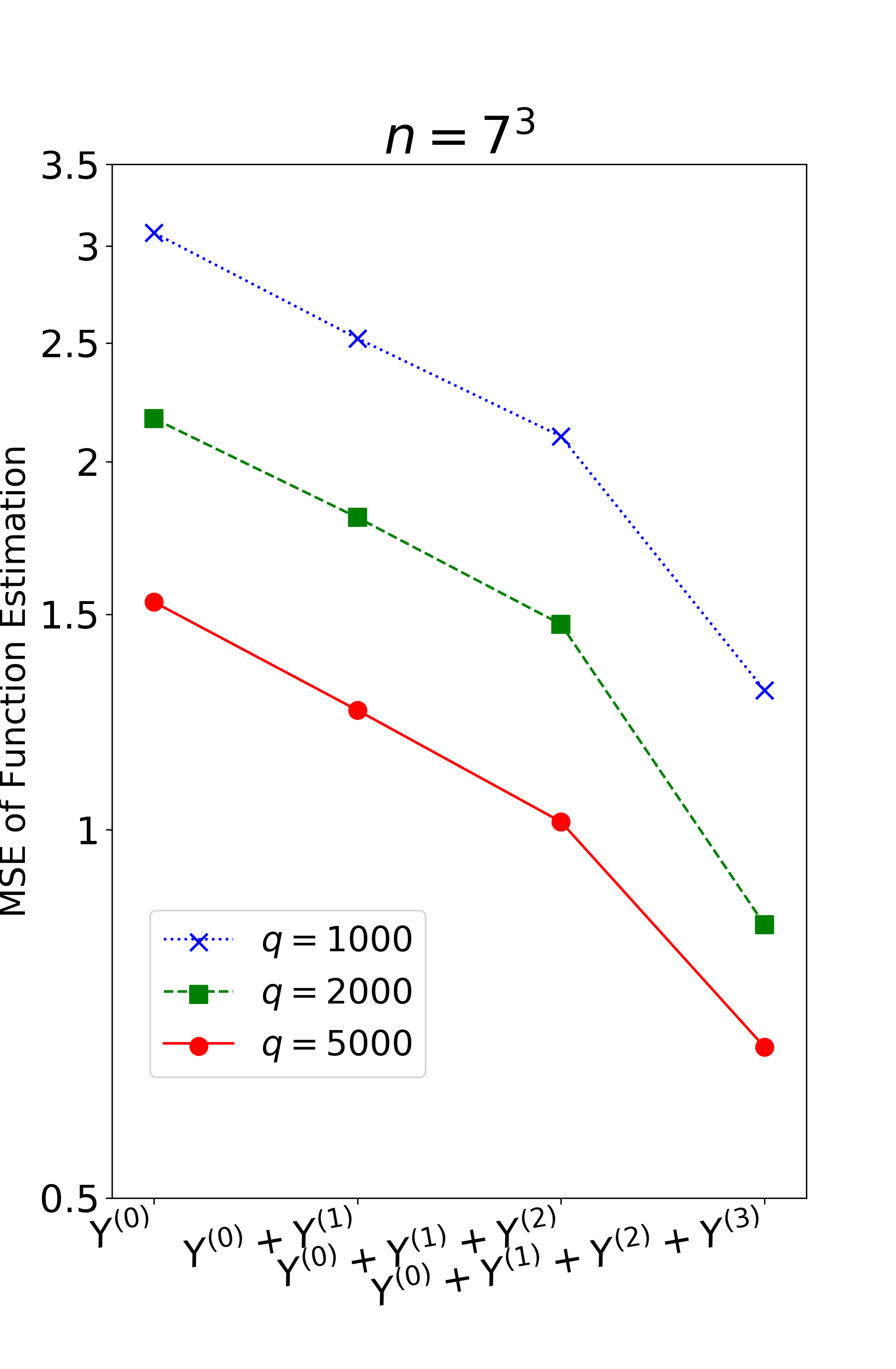
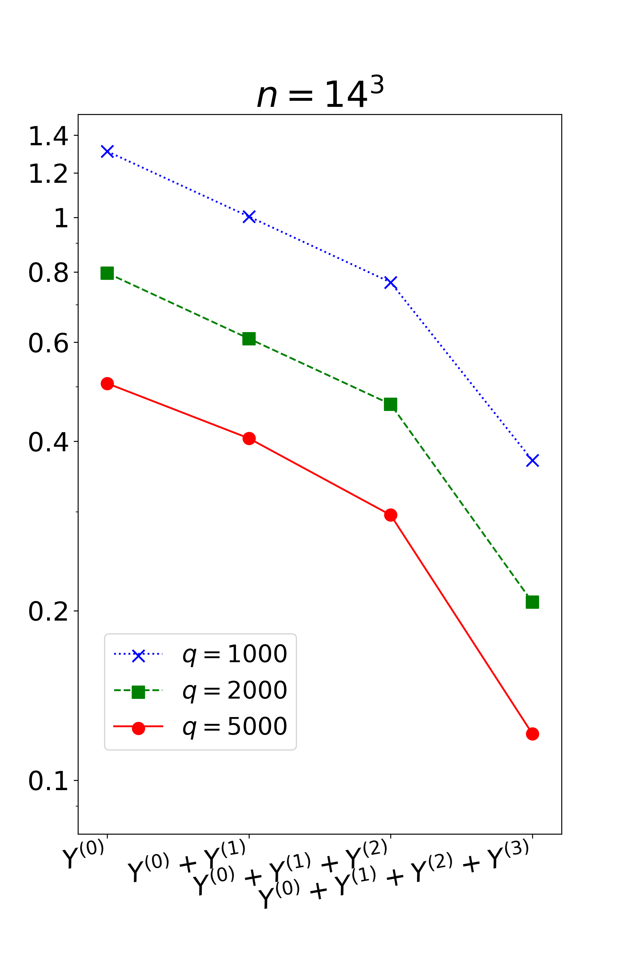
Figure 1: Estimation error of our estimator incorporating different levels of gradient information, for the stochastic simulation example. The $y$-axis is in the log scale.

We study a stochastic simulation application to motivate models (1) and (2). Let $h({\bf{t}},\omega)$ be the response of a stochastic simulation, which has a design point ${\bf{t}}\in\mathcal{X}^{d}$ and a random variable $\omega$. It is of interest to build fast and accurate estimation for $f_{0}({\bf{t}})=\mathbb{E}_{\omega}[h({\bf{t}},\omega)]$ (Chen et al., 2013; Glasserman, 2013). At each replication $k=1,\ldots,q$, the stochastic simulation has a different random variable $\omega_{k}$. A user can select design ${\bf{t}}^{(0)}$ and run the stochastic simulation to obtain a response $Y_{k}({\bf{t}}^{(0)})=h({\bf{t}}^{(0)},\omega_{k})=f_{0}({\bf{t}}^{(0)})+\epsilon^{(0)}_{k}$, where $\epsilon^{(0)}_{k}$ is i.i.d. centered simulation noise. In practice, it is common to average responses to reduce the variance of simulation noises, i.e., let $Y^{(0)}=[Y_{1}({\bf{t}}^{(0)})+Y_{2}({\bf{t}}^{(0)})+\cdots+Y_{q}({\bf{t}}^{0})]/q$, where $q$ is the number of simulation replications and is at the order of hundreds or thousands. Then the response $Y^{(0)}$ follows model (1), where $\epsilon^{(0)}$ is the averaged simulation noise. Under regularity conditions ensuring the interchange of expectation and differentiation (L’Ecuyer, 1990), the infinitesimal perturbation analysis (IPA) gives the gradient estimator of $f_{0}({\bf{t}})$ that follows model (2),

$$Y^{(j)}=\frac{\partial}{\partial t_{j}}h({\bf{t}}^{(j)},\omega),\quad{\bf{t}}^{(j)}\in\mathcal{X}^{d},\ j=1,\ldots,p,\ 1\leq p\leq d.$$

The IPA estimator is unbiased, $\mathbb{E}_{\omega}[Y^{(j)}]=\partial f_{0}/\partial t_{j}$ (Glasserman, 2013), and satisfies the error structure (3) if the replication number $q=O(n^{\Upsilon})$ (Chen et al., 2013). We provide the details of a stochastic simulation in Section 4.1. The results are reported in Figure 1, which shows the mean-squared errors (MSEs) for varying sample size $n$, replication number $q$, and different methods: stochastic kriging with only function data (i.e., $p=0$), our estimator with function and one type of gradient data (i.e., $p=1$), two types of gradient data (i.e., $p=2$), the full gradient data (i.e., $p=3$). It is clear that MSEs significantly decrease via incorporating mixed gradients. On the other hand, the computational cost for obtaining the gradient estimator is relatively low, as calculating the IPA estimator $Y^{(j)}$ does not need any new replication of simulation. In contrast, getting a new function response $Y^{(0)}$ requires $q$ new replications of the stochastic simulation, and each replication could take a high cost.

2.2 Reproducing kernel for mixed gradients

We briefly review some basic facts about RKHS. Interested readers are referred to Aronszajn (1950) and Wahba (1990) for further details. Let $K$ be a Mercer kernel that is a symmetric positive semi-definite and square-integrable function on $\mathcal{X}\times\mathcal{X}$. It can be uniquely identified with the Hilbert space $\mathcal{H}_{1}$ that is the completion of $\{K(t,\cdot):t\in\mathcal{X}\}$ under the inner product $\left\langle\sum_{i}c_{i}K(t_{i},\cdot),\sum_{j}c_{j}K(t_{j},\cdot)\right\rangle_{\mathcal{H}_{1}}=\sum_{i,j}c_{i}c_{j}K(t_{i},t_{j})$. Most commonly used kernels are differentiable, which we shall assume in what follows. In particular, we assume that

$$\frac{\partial^{2}}{\partial t\partial t^{\prime}}K(t,t^{\prime})\in\mathcal{C}(\mathcal{X}\times\mathcal{X}).$$ (7)

where $\mathcal{C}(\cdot)$ is the space of continuous functions. Let the kernel $K_{d}((t_{1},\ldots,t_{d})^{\top},(t_{1}^{\prime},\ldots,t_{d}^{\prime})^{\top})=K(t_{1},t_{1}^{\prime})\cdots K(t_{d},t_{d}^{\prime})$. Then $K_{d}(\cdot,\cdot)$ is the kernel corresponding to the RKHS $(\mathcal{H},\|\cdot\|_{\mathcal{H}})$ in (5); see, e.g., Aronszajn (1950). The condition (7) together with the continuity of $\langle\cdot,\cdot\rangle_{\mathcal{H}}$ yield that for any $g\in\mathcal{H}$, $\partial g({\bf{t}})/\partial t_{j}=\partial\langle g,K_{d}({\bf{t}},\cdot)\rangle_{\mathcal{H}}/\partial t_{j}=\left\langle g,\partial K_{d}({\bf{t}},\cdot)/\partial t_{j}\right\rangle_{\mathcal{H}}.$ Thus, the gradient $\partial g({\bf{t}})/\partial t_{j}$ is a bounded linear functional in $\mathcal{H}$ and has a representer $\partial K_{d}({\bf{t}},\cdot)/\partial t_{j}$. By the spectral theorem, the kernel function $K$ admits an eigenvalue decomposition:

$$K(t,t^{\prime})=\sum_{\nu\geq 1}\lambda_{\nu}\psi_{\nu}(t)\psi_{\nu}(t^{\prime}),$$ (8)

where $\lambda_{1}\geq\lambda_{2}\geq\cdots\geq 0$ are eigenvalues and $\{\psi_{\nu}:\nu\geq 1\}$ are the corresponding eigenfunctions. For example, $\lambda_{\nu}\asymp\nu^{-2m}$ for $\mathcal{W}_{2}^{m}(\mathcal{X})$ under the Lebesgue measure (Wahba, 1990).

3 Main Results

We present a new approach for nonparametric estimation via mixed gradients and develop a fast algorithm. Then we derive a new theory and show a behavior universal to this class of estimation problems.

3.1 Estimation via mixed gradients

We propose a new approach to combine two different sources of information for estimation. The first source of information is mixed gradients, which often suggest certain basic forms for the relationship between the variables. The second source of information is observed function data on the values of the variables. Assuming the function $f_{0}$ in (4) is smooth in $\mathcal{H}$, we impose the empirical loss of mixed gradients as a penalty. The mixed gradients and observed function data are then brought in to find the function $\widehat{f}_{n}$, which satisfies the assumed smoothness and best explains the observed data,

$$\widehat{f}_{n}({\bf{t}})=\underset{\|f\|_{\mathcal{H}}\leq R}{\arg\min} \left\{\frac{1}{n}\sum_{i=1}^{n}\left[y_{i}^{(0)}-f({\bf{t}}_{i}^{(0)})\right]^{2}+\sum_{j=1}^{p}w_{j}\cdot\frac{1}{n}\sum_{i=1}^{n}\left[y_{i}^{(j)}-\frac{\partial f}{\partial t_{j}}({\bf{t}}_{i}^{(j)})\right]^{2}\right\}.$$ (9)

The $R\geq 0$ is an appropriately chosen Hilbert radius, and $w_{j}\geq 0$ is a weight parameter, where a natural choice is $w_{j}=\sigma_{0}^{2}/\sigma_{j}^{2}$. If $\sigma^{2}_{0}$ and $\sigma^{2}_{j}$ are unknown, we can replace them with consistent estimators for the variances (Hall et al., 1990).

Theorem 1.

Assume that kernel $K$ satisfies the differentiability condition (7). Then there exists a unique minimizer $\widehat{f}_{n}({\bf{t}})$ of (9). Moreover, the minimizer is in a finite-dimensional space; there exist coefficients ${\bm{\alpha}}_{j}=(\alpha_{1j},\ldots,\alpha_{nj})^{\top}\in\mathbb{R}^{n}$ for $j=0,1,\ldots,p$ such that,

$$\widehat{f}_{n}({\bf{t}})=\sum_{i=1}^{n}\alpha_{i0}K_{d}({\bf{t}}_{i}^{(0)},{\bf{t}})+\sum_{j=1}^{p}\sum_{i=1}^{n}\alpha_{ij}\frac{\partial K_{d}}{\partial t_{j}}({\bf{t}}_{i}^{(j)},{\bf{t}}).$$

This theorem is a generalization of the well-known representer lemma for smoothing splines (Wahba, 1990). It in effect turns an infinity-dimensional optimization problem into an optimization problem over finite number of coefficients. We will devise a fast algorithm for this optimization in Section 3.2 and show its scalability for large data.

The estimator (9) is different from existing methods of incorporating gradients. For example, Morris et al. (1993) proposed a stationary Gaussian process to combine noiseless gradients, whereas the estimator (9) applies to noisy gradients. Hall and Yatchew (2007) studied a regression-kernel estimator to incorporate noisy derivatives and required special structures on the observed derivatives. However, the estimator (9) can incorporate all types of estimated or observed mixed gradients. Hall and Yatchew (2010) used a series-type estimator but could have a curse of dimensionality problem. In contrast, (9) can scale up to a large dimension $d$. Chen et al. (2013) considered a stochastic kriging method, where the correlation coefficients between gradients and function data are required to be estimated. Differently, it is unnecessary to estimate such correlations for implementing (9). Moreover, we will demonstrate that the estimator (9) outperforms competing alternatives through numerical examples in Section 4.

3.2 Computational algorithm

This section develops a fast algorithm for computing the minimizer $\widehat{f}_{n}({\bf{t}})$ in Theorem 1. The minimizer $\widehat{f}_{n}({\bf{t}})$ in Theorem 1 can be further written as, for any ${\bf{t}}\in\mathcal{X}^{d}$,

$$\widehat{f}_{n}({\bf{t}})=\tilde{\mathbf{\Psi}}_{d}({\bf{t}})^{\top}\tilde{{\bf{c}}}_{0}+\sum_{j=1}^{p}\frac{\partial\tilde{\mathbf{\Psi}}_{d}({\bf{t}})^{\top}\tilde{{\bf{c}}}_{j}}{\partial t_{j}},$$ (10)

where $\tilde{\mathbf{\Psi}}_{d}({\bf{t}})=\left[\tilde{\mathbf{\Psi}}^{\otimes_{1}}(t_{1})^{\top},\ldots,\tilde{\mathbf{\Psi}}^{\otimes_{1}}(t_{d})^{\top},\tilde{\mathbf{\Psi}}^{\otimes_{2}}(t_{1},t_{2})^{\top},\ldots,\tilde{\mathbf{\Psi}}^{\otimes_{r}}(t_{d-r+1},t_{d-r+2},\ldots,t_{d})^{\top}\right]^{\top}$, and $\widetilde{\mathbf{\Psi}}^{\otimes_{1}}(t)$ is an infinite-dimensional vector with the $\nu$th element equal to $\sqrt{\lambda_{\nu}}\psi_{\nu}(X)$ for $\nu\geq 1$, and $\mathbf{\Psi}^{\otimes_{2}}(t_{i},t_{j})=\mathbf{\Psi}^{\otimes_{1}}(t_{i})\otimes\mathbf{\Psi}^{\otimes_{1}}(t_{j})$, and so on. Here $\tilde{{\bf{c}}}_{j}=\Big{[}\widetilde{\mathbf{\Psi}}_{d}({\bf{t}}^{(j)}_{1}),\ldots,\widetilde{\mathbf{\Psi}}_{d}({\bf{t}}^{(j)}_{n})\Big{]}{\bm{\alpha}}_{j}$ is the infinite-dimensional coefficient vector, $j=0,1,\ldots,p$.

The key idea is to employ the random feature mapping (Rahimi and Recht, 2007; Dai et al., 2022) to approximate the kernel function, which enables us to construct a projection operator between the RKHS and the original predictor space. Specifically, if the kernel functions that generate $\mathcal{H}_{1}$ are shift-invariant, i.e., $K(t,t^{\prime})=K(t-t^{\prime})$, and integrate to one, i.e., $\int_{\mathcal{X}}K(t-t^{\prime})d(t-t^{\prime})=1$, then the Bochner’s theorem (Bochner, 1934) states that such kernel functions satisfy the Fourier expansion:

$$K(t-t^{\prime}) =\int_{\mathbb{R}}p(w)\exp\left\{\sqrt{-1}w(t-t^{\prime})\right\}dw,$$

where $p(w)$ is a probability density defined by

$$p(w)=\int_{\mathcal{X}}K(t)e^{-2\pi\sqrt{-1}wt}dt.$$

We note that many kernel functions are shift-invariant and integrate to one. Examples include the Matérn kernel, $K(t,t^{\prime})=\tilde{\tau}_{1}(1+|t-t^{\prime}|/\tau_{1}+|t-t^{\prime}|^{2}/3\tau_{1}^{2})e^{-|t-t^{\prime}|/\tau_{1}}$, the Laplacian kernel, $K(X,X^{\prime})=\tilde{\tau}_{2}e^{-|X-X^{\prime}|/\tau_{2}}$, the Gaussian kernel, $K(X,X^{\prime})=\tilde{\tau}_{3}e^{-\tau_{3}^{2}|X-X^{\prime}|^{2}/2}$, and the Cauchy kernel, $K(X,X^{\prime})=\tilde{\tau}_{4}(1+\tau_{4}^{2}|X-X^{\prime}|^{2})^{-1}$, where $\tilde{\tau}_{1},\tilde{\tau}_{2},\tilde{\tau}_{3},\tilde{\tau}_{4}$ are the normalization constants, and $\tau_{1},\tau_{2},\tau_{3},\tau_{4}$ are the scaling parameters. It is then shown that (Rahimi and Recht, 2007) the minimizer in Theorem 1 can be approximated by,

$$\widehat{f}_{n}({\bf{t}})=\mathbf{\Psi}_{d}({\bf{t}})^{\top}{{\bf{c}}_{0}}+\sum_{j=1}^{p}\frac{\partial\mathbf{\Psi}_{d}({\bf{t}})^{\top}{{\bf{c}}_{j}}}{\partial t_{j}},$$

where $\mathbf{\Psi}_{d}({\bf{t}})=\left[\mathbf{\Psi}^{\otimes_{1}}(t_{1})^{\top},\ldots,\mathbf{\Psi}^{\otimes_{1}}(t_{d})^{\top},\mathbf{\Psi}^{\otimes_{2}}(t_{1},t_{2})^{\top},\ldots,\mathbf{\Psi}^{\otimes_{r}}(t_{d-r+1},t_{d-r+2},\ldots,t_{d})^{\top}\right]^{\top}$, and $\mathbf{\Psi}^{\otimes_{1}}(t_{j})=\left[\tilde{\psi}_{1}(t_{j}),\ldots,\tilde{\psi}_{s}(t_{j})\right]^{\top}\in\mathbb{R}^{s}$ is a vector of $s$ Fourier bases with the frequencies drawn from the density $p(w)$, i.e.,

$$\omega_{j,\nu}\overset{\text{i.i.d.}}{\sim}p(\omega),\quad\quad b_{j,\nu}\overset{\text{i.i.d.}}{\sim}\textrm{Uniform}[0,2\pi],$$ (11)

$$\tilde{\psi}_{\nu}(t_{j})=\sqrt{\frac{2}{s}}\cos(t_{j}\omega_{j,\nu}+b_{j,\nu}),\quad\quad j=1,\ldots,d,\;\nu=1,\ldots,s,$$

and $\mathbf{\Psi}^{\otimes_{2}}(t_{i},t_{j})=\mathbf{\Psi}^{\otimes_{1}}(t_{i})\otimes\mathbf{\Psi}^{\otimes_{1}}(t_{j})\in\mathbb{R}^{s^{2}}$, and so on. We write the augmented random feature vector as,

$$\mathbf{\Psi}_{(p+1)d}({\bf{t}})=\left(\mathbf{\Psi}_{d}({\bf{t}})^{\top},\frac{\partial\mathbf{\Psi}_{d}({\bf{t}})^{\top}}{\partial t_{1}},\ldots,\frac{\partial\mathbf{\Psi}_{d}({\bf{t}})^{\top}}{\partial t_{p}}\right)^{\top}.$$ (12)

Then the minimizer in Theorem 1 can be approximated by,

$$\widehat{f}_{n}({\bf{t}})=\mathbf{\Psi}_{(p+1)d}({\bf{t}})^{\top}{{\bf{c}}_{(p+1)d}}.$$ (13)

We then estimate the coefficient vector ${\bf{c}}_{(p+1)d}=({\bf{c}}_{0}^{\top},{\bf{c}}_{1}^{\top},\ldots,{\bf{c}}_{p}^{\top})^{\top}$ via minimizing the following convex objective function,

$$\frac{1}{n}\sum_{i=1}^{n}\left[y_{i}^{(0)}-\bar{y}^{(0)}-\widehat{f}_{n}({\bf{t}}_{i}^{(0)})\right]^{2}+\sum_{j=1}^{p}w_{j}\cdot\frac{1}{n}\sum_{i=1}^{n}\left[y_{i}^{(j)}-\bar{y}^{(j)}-\frac{\partial\widehat{f}_{n}}{\partial t_{j}}({\bf{t}}_{i}^{(j)})\right]^{2}+\lambda\sum_{j=0}^{p}\|{\bf{c}}_{j}\|_{2}^{2}.$$ (14)

Here $\bar{y}^{(0)}=\sum_{i=1}^{n}y^{(0)}_{i}/n$ and $\bar{y}^{(j)}=\sum_{i=1}^{n}y^{(j)}_{i}/n$ are the empirical means for function data and mixed gradients $j=0,1,\ldots,p$, respectively, and $\lambda\geq 0$ is the penalty parameter. We remark that the penalty in (14) is different from the kernel ridge regression penalty (Wainwright, 2019), which takes the form $\|\Psi_{(p+1)d}({\bf{t}})^{\top}{{\bf{c}}_{(p+1)d}}\|_{\mathcal{H}}^{2}$. Since the random feature mapping generally cannot form an orthogonal basis, there is no closed-form representation of the RKHS norms $\|\Psi_{(p+1)d}({\bf{t}})^{\top}{{\bf{c}}_{(p+1)d}}\|_{\mathcal{H}}^{2}$ in our setting. As a result, the kernel ridge regression penalty is difficult to implement, and instead we adopt the $L_{2}$ penalty in (14) that is easy for computing. We choose the smoothing parameter $\lambda$ in (9) by generalized cross-validation (GCV) (Golub et al., 1979). Let $A(\lambda)$ be the influence matrix as $\widehat{y}=A(\lambda)y$, where $y$ is the vector of function and gradient data $y=(y_{1}^{(0)},\ldots,y^{(0)}_{n},\ldots,y^{(p)}_{1},\ldots,y^{(p)}_{n})^{\top}$, and $\widehat{y}$ is the estimate, $\widehat{y}=(\widehat{f}_{n}({\bf{t}}_{1}^{(0)}),\ldots,\widehat{f}_{n}({\bf{t}}_{n}^{(0)}),\ldots,\partial\widehat{f}_{n}/\partial t_{p}({\bf{t}}_{1}^{(p)}),\ldots,\partial\widehat{f}_{n}/\partial t_{p}({\bf{t}}_{n}^{(p)}))^{\top}$. Then GCV selects $\lambda\geq 0$ by minimizing the following risk,

$$\text{GCV}(\lambda)=\frac{\|\widehat{y}-y\|^{2}}{[n^{-1}\text{tr}(I-A(\lambda))]^{2}}.$$

The use of random feature mapping achieves potentially substantial dimension reduction. More specifically, the estimator in (13) only requires to learn the finite-dimensional coefficient ${\bm{\alpha}_{j}}$ for $j=0,1,\ldots,p$, compared to the estimator in (10) that involves an infinite-dimensional vector $\widetilde{{\bf{c}}}_{p}$. Rudi and Rosasco (2017) showed that the random feature mapping obtains an optimal bias-variance tradeoff if $s$ scales at a certain rate and $s/n\to 0$ when $n$ grows. We note that the random feature mapping also efficiently reduces the computational complexity. Given any $(d,r,p)$, the computation complexity of the estimator in (13) is only $O(ns^{2})$, compared to the computation complexity of the kernel estimator in Theorem 1 that is $O(n^{3})$. The saving of the computation is substantial if $s/n\to 0$ as $n$ grows.

Algorithm 1 Estimation via mixed gradients.

1:  Input: Function data $\{({\bf{t}}_{i}^{(0)},y_{i}^{(0)}):i=1,\ldots,n\}$, mixed gradients $\{({\bf{t}}_{i}^{(j)},y_{i}^{(j)}):i=1,\ldots,n;j=1,\ldots,p\}$, weight parameters $\{w_{j}:j=1,\ldots,p\}$.

2:  Step 1: Sample $d$ of i.i.d. $s$-dimensional random features $\{w_{\nu},b_{\nu}\}_{\nu=1}^{s}$ by (11), and construct the augmented random feature vector $\mathbf{\Psi}_{(p+1)d}({\bf{t}})$ by (12).

3:  Step 2: Solve the coefficient vector ${\bf{c}}_{(p+1)d}$ by (14).

4:  Output: Function estimate $\widehat{f}_{n}({\bf{t}})$ in (13).

We summarize the above estimation procedure in Algorithm 1.

3.3 Minimax optimality

We show that our proposed estimator achieves optimality. Suppose that design points ${\bf{t}}^{(0)}$ in (1) and ${\bf{t}}^{(j)}$s in (2) are independently drawn from $\Pi^{(0)}$ and $\Pi^{(j)}$s, respectively, where $\Pi^{(0)}$ and $\Pi^{(j)}$s have densities bounded away from zero and infinity. We first present a minimax lower bound in the presence of mixed gradients.

Theorem 2.

Assume that $\lambda_{\nu}\asymp\nu^{-2m}$ for some $m>3/2$. Under the regression models (1) and (2) where $f_{0}$ follows the SS-ANOVA model (4). Then under the general error structure (3), there exists a constant $c$ such that

$$\underset{n\to\infty}{\lim\inf}\inf_{\tilde{f}}\sup_{f_{0}\in\mathcal{H}}\mathbb{P} \left\{\int_{\mathcal{X}^{d}}\left[\tilde{f}({\bf{t}})-f_{0}({\bf{t}})\right]^{2}d{\bf{t}}\geq c\left(\left[n(\log n)^{1-(d-p)\wedge r}\right]^{-\frac{2m}{2m+1}}\mathbbm{1}_{0\leq p<d}\right.\right.$$

$$\left.\left.\quad\quad+\left[n^{-\frac{2mr}{(2m+1)r-2}}\mathbbm{1}_{r\geq 3}+n^{-1}(\log n)^{r-1}\mathbbm{1}_{r<3}\right]\mathbbm{1}_{p=d}\vphantom{\int_{\mathcal{X}^{d}}\left\{\tilde{f}({\bf{t}})-f_{0}({\bf{t}})\right\}^{2}d{\bf{t}}}\right)\right\}>0,$$

where the infimum of $\tilde{f}$ is taken over all measurable functions of the data.

This lower bound is new in the literature, and its proof is established via Fano’s lemma (Tsybakov, 2009). Next, we show that the lower bound is attainable via our estimator.

Theorem 3.

Assume that $\lambda_{\nu}\asymp\nu^{-2m}$ for some $m>3/2$. Under the regression models (1) and (2) where $f_{0}$ follows the SS-ANOVA model (4). Then under the general error structure (3), the estimator $\widehat{f}_{n}$ defined by (9) satisfies

$$\lim_{C\to\infty}\underset{n\to\infty}{\lim\sup} \sup_{f_{0}\in\mathcal{H}}\mathbb{P}\left\{\int_{\mathcal{X}^{d}}\left[\widehat{f}_{n}({\bf{t}})-f_{0}({\bf{t}})\right]^{2}d{\bf{t}}\right.\leq C\left(\left[n(\log n)^{1-(d-p)\wedge r}\right]^{-\frac{2m}{2m+1}}\mathbbm{1}_{0\leq p<d}\right.$$

$$\left.\left.\quad\quad\quad\quad+\left[n^{-\frac{2mr}{(2m+1)r-2}}\mathbbm{1}_{r\geq 3}+n^{-1}(\log n)^{r-1}\mathbbm{1}_{r<3}\right]\mathbbm{1}_{p=d}\vphantom{\left[n(\log n)^{1-(d-p)\wedge r}\right]^{-2m/(2m+1)}}\right)\vphantom{\int_{\mathcal{X}^{d}}\left\{\tilde{f}({\bf{t}})-f_{0}({\bf{t}})\right\}^{2}d{\bf{t}}}\right\}=1.$$

Here the tuning parameter $\lambda$ in (14) is chosen by $\lambda\asymp\left[n(\log n)^{1-(d-p)\wedge r}\right]^{-2m/(2m+1)}$ when $0\leq p<d$, and $\lambda\asymp n^{-(2mr-2)/[(2m+1)r-2]}$ when $p=d,r\geq 3$, and $\lambda\asymp(n\log n)^{-(2m-1)/2m}$ when $p=d,r=2$, and $\lambda\asymp n^{-(m-1)/m}$ when $p=d$, $r=1$.

The proof of Theorem 3 relies on several techniques from empirical process and stochastic process theory, including the linearization method and operator gradients.

Theorems 2 and 3 together immediately imply that the minimax optimal rate for estimating $f_{0}\in\mathcal{H}$ is

$$\left[n(\log n)^{1-(d-p)\wedge r}\right]^{-\frac{2m}{2m+1}}\mathbbm{1}_{0\leq p<d}$$ (15)

$$\quad\quad\quad+\left[n^{-\frac{2mr}{(2m+1)r-2}}\mathbbm{1}_{r\geq 3}+n^{-1}(\log n)^{r-1}\mathbbm{1}_{r<3}\right]\mathbbm{1}_{p=d}.$$

This result connects with two strands of literature–estimating SS-ANOVA models without gradient information, and estimating nonparametric functions with derivatives.

First, in the case of estimating SS-ANOVA models without gradient information, the result in (15) recovers the rate known in the literature (see, e.g., Lin (2000)),

$$\left[n(\log n)^{1-r}\right]^{-\frac{2m}{2m+1}}.$$

For a high-order interaction $r$, the exponential term $(\log n)^{r-1}$ above makes the SS-ANOVA models impractical, which phenomenon is called the curse of interaction. Surprisingly, the result in (15) shows that incorporating gradient data mitigates the curse of interaction. For example, when $d-r\leq p\leq d-1$, the rate given by (15) becomes,

$$\left[n(\log n)^{1-(d-p)}\right]^{-\frac{2m}{2m+1}}.$$ (16)

This rate is identical to the minimax optimal rate for estimating a $(d-p)$-interaction model without gradient information (Lin, 2000). When increasing $p$ types of gradient data to $(p+1)$ types, the rate given by (16) is accelerated at the order of $(\log n)^{-\frac{2m}{2m+1}}$, where $p\geq d-r$ and $p+1\leq d-1$. Moreover, when $p=d-1$, the rate given by (16) is $n^{-\frac{2m}{2m+1}}$, which coincides with the optimal rate for estimating additive models without gradient information (Stone, 1985). The result in (15) indicates a phase transition from $0\leq p<d$ to $p=d$. Specifically, the rate with full gradient $p=d$ is further improved compared to that with $p\leq d-1$. We also note that when the SS-ANOVA models have full interaction with $r=d$, the result in (15) yields the special result in (6).

Second, in the case of estimating functions with derivatives, Hall and Yatchew (2007) pioneered in proposing a regression-kernel method for incorporating various derivative data under random design and i.i.d. errors. Hall and Yatchew (2007) proved that when the derivative data are first-order partial derivatives (i.e., mixed gradient), their estimator achieves the rate $n^{-\frac{2m}{2m+d-1}}$ (e.g., their Theorem 3), which converges slower than the optimal rate given by (15) when $d\geq 2$ and has the curse of dimensionality when $d$ is large. Our new result in (15) shows that gradient information is useful for the scalability of nonparametric modeling in high dimensions when employing the SS-ANOVA models.

Moreover, the optimal rate in (15) also holds for deterministic designs. For example, the design points ${\bf{t}}^{(0)}$ in (1) and ${\bf{t}}^{(j)}$s in (2) can be equally spaced in $\mathcal{X}^{d}$ rather than independently drawn from distributions $\Pi^{(0)}$ and $\Pi^{(j)}$s, respectively. The results for deterministic designs are relegated to the Appendix.

4 Aplications

In this section, we demonstrate the aspects of our theory and method via various applications. We study a stochastic simulation example in Section 4.1, and an economics example in Section 4.2. We analyze a real data experiment of ion channel in Section 4.3.

4.1 Call option pricing with stochastic simulations

We discussed a motivating example of stochastic simulation in Section 2.1. Now we consider a detailed stochastic simulation of the call option pricing. The Black-Scholes stochastic differential equation is commonly used to model stock price $S_{T}$ at time $T$ through

$$dS_{T}=r_{*}S_{T}dT+\sigma_{*}S_{T}dW_{T},T\geq 0,$$

where $W_{T}$ is the Wiener process, $r_{*}$ is the risk-free rate, and $\sigma_{*}$ is the volatility of the stock price. The equation has a closed-form solution: $S_{T}=S_{0}\exp\{(r_{*}-\frac{1}{2}\sigma_{*}^{2})T+\sigma_{*}\sqrt{T}\omega\}$ with the standard normal variable $\omega$ and initial stock price $S_{0}$. The European call option is the right to buy a stock at the prespecified time $T$ with a prespecified price $P_{0}$. The value of the European option is

$$h({\bf{t}},\omega)=e^{-rT}(S_{T}-P_{0})_{+},$$

where ${\bf{t}}=(S_{0},r_{*},\sigma_{*})$. Our goal is to estimate the expected net present value of the option with fixed $T,P_{0}$: $f_{0}({\bf{t}})=\mathbb{E}_{\omega}[h({\bf{t}},\omega)]$. It is seen that $f_{0}({\bf{t}})$ follows the SS-ANOVA model (4). In the experiment, we fix $T=1$, $P_{0}=100$, and choose the design ${\bf{t}}$ from equally spaced points from $S_{0}\in[80,120]$, $r_{*}\in[0.01,0.05]$, and $\sigma_{*}\in[0.2,1]$ with the sample size $n=7^{3},14^{3},21^{3}$. The end points of each interval are always included. To address the impact of stochastic simulation noise, we simulate $q=1000,2000,5000$ i.i.d. replications of $S_{T}$ at each design point and then average the responses. Independent sampling is used across design points. It is known that IPA estimators for the gradient: $\partial f_{0}/\partial S_{0}$, $\partial f_{0}/\partial r_{*}$, $\partial f_{0}/\partial\sigma_{*}$ are given by Glasserman (2013),

$$Y^{(1)} =e^{-r_{*}T}\frac{S_{T}}{S_{0}}\cdot{\mathbf{1}}\{S_{T}\geq P_{0}\},$$ (17)

$$Y^{(2)} =-TY^{(0)}+e^{-r_{*}T}TS_{T}\cdot{\mathbf{1}}\{S_{T}\geq P_{0}\},$$

$$Y^{(3)} =e^{-r_{*}T}\frac{1}{\sigma_{*}}\left[\log\left(\frac{S_{T}}{S_{0}}\right)-\left(r_{*}+\frac{1}{2}\sigma_{*}^{2}\right)T\right]S_{T}\cdot{\mathbf{1}}\{S_{T}\geq P_{0}\}.$$

The IPA estimators (17) are unbiased, $\mathbb{E}_{\omega}[Y^{(1)}]=\partial f_{0}/\partial S_{0},\mathbb{E}_{\omega}[Y^{(2)}]=\partial f_{0}/\partial r_{*}$, $\mathbb{E}_{\omega}[Y^{(3)}]=\partial f_{0}/\partial\sigma_{*}$. Then the error correlation only exists for function and gradient data at the same design, not between components at different design points. Hence the error structure (3) is satisfied. In this example, obtaining function data at a new design point requires to generate $q$ new random numbers, and solve $S_{T}$ at each of the $q$ new simulation replications. In contrast, the gradient estimator in (17) can be obtained at a negligible cost and without any new simulation.

Comparison to existing method.

Stochastic kriging (Ankenman et al., 2010) is a popular method for the mean response estimation of a stochastic simulation. We compare the estimation results of our estimator (9) incorporating gradient information and the stochastic kriging method without gradient. Consider the tensor product Matérn kernel,

$$\prod_{j=1}^{3}\left(1+|t_{j}-t^{\prime}_{j}|/\tau_{j}+|t_{j}-t^{\prime}_{j}|^{2}/3\tau_{j}^{2}\right)\exp\left(-|t_{j}-t^{\prime}_{j}|/\tau_{j}\right).$$ (18)

This kernel satisfies the differentiability condition (7), where lengthscale parameters $\tau_{j}$s are chosen by the five-fold cross-validation. We use the actual output as the reference given by $f_{0}(S_{0},r_{*},\sigma_{*})=S_{0}\Phi\left(-d_{1}+\sigma_{*}\right)-100e^{-r_{*}}\Phi\left(-d_{1}\right)$ when $T=1,P_{0}=100$, where $d_{1}=\sigma_{*}^{-1}[\log 100-\log(S_{0})-(r_{*}-\sigma_{*}^{2}/2)]$ and $\Phi(\cdot)$ is the CDF of standard normal distribution. We estimate the MSE$=\mathbb{E}(\widehat{f}_{n}-f_{0})^{2}$ by a Monte Carlo sample of $10^{4}$ test points in $[80,120]\times[0.01,0.05]\times[0.2,1]$.

Figure 1 reports the MSEs for different methods: stochastic kriging with only function data (i.e., $p=0$), our estimator with different types of gradient data. The results are averaged over $1000$ simulations in each setting. It is seen that our estimator with gradient data gives a substantial improvement in estimation compared to stochastic kriging without gradient. For example, the MSE of $n=7^{3},q=1000$ with full gradient (i.e., $p=3$) is comparable to the MSE of $n=14^{3},q=1000$ without gradient (i.e., $p=0$). Since it needs little additional cost to estimate gradients by (17), our estimator essentially saves the computational cost of sampling at new designs. It is also seen that a faster convergence rate is obtained when incorporating all gradient data (i.e., $p=3$) compared to $p\leq 2$.

Table 1: The ratios of MSE with two types of gradient data (i.e., $p=2$) relative to MSE with only function data (i.e., $p=0$), for the example in Section 4.1.

$n$	$q=10^{3}$	$q=2000$	$q=5000$
$7^{3}=343$	$0.6818$	$0.6789$	$0.6612$
$14^{3}=2744$	$0.5850$	$0.5848$	$0.5835$
$21^{3}=9261$	$0.5484$	$0.5483$	$0.5294$

Table 1 reports the ratios of the MSE of our estimator with two types of gradient data (i.e., $p=2$) relative to the MSE of stochastic kriging with only function data (i.e., $p=0$). It is seen that incorporating gradient data leads to a faster convergence rate.

4.2 Cost estimation in economics

We consider an economic problem of the cost function estimation. Write the cost function $f_{0}({\bf{t}})=f_{0}(t_{1},\ldots,t_{d})$, where $t_{d}$ denotes the level of output and $(t_{1},\ldots,t_{d-1})$ represent the prices of $d-1$ factor inputs. The Cobb-Douglas production function (Varian, 1992) yields that

$$f_{0}(t_{1},\ldots,t_{d})=c_{0}^{-\frac{1}{c}}\prod_{1\leq j\leq d-1}\left(\frac{c}{c_{j}}\right)^{\frac{c_{j}}{c}}\prod_{1\leq j\leq d-1}t_{j}^{\frac{c_{j}}{c}}t_{d}^{\frac{1}{c}}.$$

Here $c_{0}$ is the efficiency parameter, $c_{1},\ldots,c_{d-1}$ are elasticity parameters, and $c=c_{1}+\cdots+c_{d-1}$. Our goal is to estimate the cost function $f_{0}({\bf{t}})$. The function data of $f_{0}({\bf{t}})$ are observed at design ${\bf{t}}^{(0)}\in\mathcal{X}^{d}$. The gradient data of $f_{0}({\bf{t}})$ with respect to input prices are the quantities of factor inputs that are also observable (Hall and Yatchew, 2007),

$$Y^{(j)}=\frac{\partial}{\partial t_{j}}f_{0}({\bf{t}}^{(j)})+\epsilon^{(j)},\quad{\bf{t}}^{(j)}\in\mathcal{X}^{d},\ j=1,\ldots,d-1.$$

Here ${\bf{t}}^{(j)}={\bf{t}}^{(0)}\in\mathcal{X}^{d}$ for $1\leq j\leq d-1$ that typically follows a random design. Moreover, the observational errors are usually assumed to be i.i.d. (Hall and Yatchew, 2007) and hence satisfy the error structure (3). Since the gradient data about $\partial f_{0}/\partial t_{d}$ is not usually observable, it motivates our modeling of $p\in\{1,\ldots,d\}$ in model (2). Clearly, $f_{0}({\bf{t}})$ in this example follows the SS-ANOVA model (4). In the experiment, we consider $d=3$ and fix $t_{3}=1$ since the cost function is homogeneous of degree one in $(t_{1},t_{2},t_{3})$, that is $f_{0}(t_{1},t_{2},t_{3},t_{4})=t_{3}f_{0}(t_{1}/t_{3},t_{2}/t_{3},1,t_{4})$. The data are generated through,

$$Y^{(0)} =f_{0}(t_{1},t_{2},1,t_{4})+\epsilon^{(0)},\quad Y^{(j)} =\frac{\partial f_{0}(t_{1},t_{2},1,t_{4})}{\partial t_{j}}+\epsilon^{(j)}\mbox{ for }j=1,2,$$

where $c_{0}=1,c_{1}=0.8,c_{2}=0.7,c_{3}=0.6$, and the designs ${\bf{t}}^{(j)},j=0,1,2$ follow the i.i.d. uniform distribution in $[0.5,1.5]^{3}$. Suppose that $\epsilon^{(j)},j=0,1,2$ are Gaussian with zero means, standard deviations $0.35$, and correlation $\rho$. We consider varying sample size $n=100,200,500,1000$ and correlation $\rho=0,0.4,0.9$.

Comparison to existing method.

Hall and Yatchew (2007) proposed a regression-kernel method for incorporating gradient for cost function estimation. We compare the performance of our estimator (9) with that of Hall and Yatchew’s estimator. For the estimator in Hall and Yatchew (2007), we follow Hall and Yatchew’s Example 3 to use the tensor product Matérn kernel (18) to average $(t_{1},t_{4})$ and $(t_{2},t_{4})$ directions locally, and then average the estimates. The MSE is estimated by a Monte Carlo sample of $10^{4}$ test points in $[0.5,1.5]^{3}$.

Table 2: MSEs of our estimator and Hall and Yatchew’s estimator incorporating different levels of data, for the example in Section 4.2. The MSEs are in the unit of $10^{-4}$.

		Our Estimator (9)	Hall and Yatchew (2007)	Our Estimator (9)
		with only $Y^{(0)}$	with $Y^{(0)}+Y^{(1)}+Y^{(2)}$	with $Y^{(0)}+Y^{(1)}+Y^{(2)}$
	$\rho=0$	$127.1471$	$61.4098$	47.4739
$n=100$	$\rho=0.4$	$128.9210$	$63.1006$	49.8963
	$\rho=0.9$	$129.6300$	$64.5989$	51.9224
	$\rho=0$	$76.6199$	$33.3001$	24.1501
$n=200$	$\rho=0.4$	$77.7602$	$35.0696$	25.5342
	$\rho=0.9$	$77.9138$	$36.2591$	27.0137
	$\rho=0$	$36.1925$	$16.3861$	9.3499
$n=500$	$\rho=0.4$	$38.0683$	$18.2355$	10.4708
	$\rho=0.9$	$38.9311$	$18.7698$	11.0498
	$\rho=0$	$21.8570$	$9.2788$	4.5364
$n=1000$	$\rho=0.4$	$22.4943$	$10.4801$	5.1468
	$\rho=0.9$	$22.9499$	$10.6193$	5.3288

Table 2 reports the MSEs for varying sample size $n$, correlation $\rho$, and different methods: our estimator with only function data (i.e., $p=0$), Hall and Yatchew’s estimator with function and gradient data (i.e., $p=2$), our estimator with function and gradient data (i.e., $p=2$). The results are averaged over $1000$ simulations in each setting. It is seen that the MSE of incorporating gradient information is significantly smaller than the MSE without gradient. Moreover, the performances of our estimator compare favorably with that of Hall and Yatchew’s estimator.

Table 3 reports the ratios of the MSE of our estimator incorporating two types of gradient data (i.e., $p=2$) relative to the MSE of Hall and Yatchew’s estimator incorporating two types of gradient data (i.e., $p=2$). It is seen that the ratio decreases with the sample size, which agrees with our theoretical finding in Section 3, since our estimator in this example converges at the rate $n^{-2m/(2m+1)}$ by Theorem 3, and Hall and Yatchew’s estimator converges at a slower rate $n^{-m/(m+1)}$.

Table 3: The ratios of MSE of our estimator with two types of gradient data (i.e., $p=2$) relative to MSE of Hall and Yatchew’s estimator with two types of gradient data (i.e., $p=2$), for the example in Section 4.2.

	$\rho=0$	$\rho=0.4$	$\rho=0.9$
$n=100$	$0.7731$	$0.7907$	$0.8038$
$n=200$	$0.7252$	$0.7281$	$0.7450$
$n=500$	$0.5706$	$0.5742$	$0.5887$
$n=1000$	$0.4889$	$0.4911$	$0.5018$

4.3 Ion channel experiment

We consider a real data example from a single voltage clamp experiment. The experiment is on the sodium ion channel of the cardiac cell membranes. The experiment output $z_{k}$ measures the normalized current for maintaining a fixed membrane potential of $-35mV$ and the input $x_{k}$ is the logarithm of time. The sample size of the ion channel experiment is $N=19$. Computer model has been used to study the ion channel experiment (Plumlee, 2017). Let $\eta(x,{\bf{t}})$ be the computer model that approximates the physical system for the ion channel experiment, where $x$ is the experiment input and ${\bf{t}}\in\mathcal{X}^{d}$ is the calibration parameter whose value are unobservable. For analyzing the ion channel experiment, the computer model is given by $\eta(x,{\bf{t}})=e_{1}^{\top}\exp(\exp(x)A({\bf{t}}))e_{4}$, where ${\bf{t}}=(t_{1},t_{2},t_{3})^{\top}\in\mathcal{X}^{d}$, $d=3$, $e_{1}=(1,0,0,0)^{\top},e_{4}=(0,0,0,1)^{\top}$, and

$$A({\bf{t}})=\left(\begin{array}[]{cccc}-t_{2}-t_{3}&t_{1}&0&0\\ t_{2}&-t_{1}-t_{2}&t_{1}&0\\ 0&t_{2}&-t_{1}-t_{2}&t_{1}\\ 0&0&t_{2}&-t_{1}\end{array}\right).$$

Our goal is to estimate the function, $f_{0}({\bf{t}})=\mathbb{E}_{(x,z)}[z-\eta(x,{\bf{t}})]^{2}$, which is useful for visualization, calibration, and understanding how well the computer model approximates the physical system in this experiment (Kennedy and O’Hagan, 2001). The function data at design ${\bf{t}}^{(0)}\in\mathcal{X}^{3}$ is generated by,

$$Y^{(0)}=\frac{1}{N}\sum_{k=1}^{N}[z_{k}-\eta(x_{k},{\bf{t}}^{(0)})]^{2},\quad\text{where }N=19.$$

The gradient of computer model, i.e., $\nabla_{{\bf{t}}}\eta(x,{\bf{t}})$, can be obtained using the chain rule-based automatic differentiation. By the cheap gradient principle (Griewank and Walther, 2008), the cost for computing $\nabla_{{\bf{t}}}\eta(x,{\bf{t}})$ is at most four or five times the cost for function evaluation $\eta(x,{\bf{t}})$ and hence, the gradient is cheap to obtain. Then the estimator for the gradient of $f_{0}({\bf{t}})$ is given by,

$$Y^{(j)}=-\frac{2}{N}\sum_{k=1}^{N}\left[z_{k}-\eta(x_{k},{\bf{t}}^{(j)})\right]\frac{\partial}{\partial t_{j}}\eta(x_{k},{\bf{t}}^{(j)}),\quad{\bf{t}}^{(j)}\in\mathcal{X}^{3},\ j=1,2,3.$$

In the experiment, we choose i.i.d. uniform designs for ${\bf{t}}^{(j)}$s, $j=0,1,2,3$ from $\mathcal{X}^{3}$ with the sample size $n=1000,2000,3000,5000$.

Table 4: MSEs of our estimator and Morris et al.’s estimator incorporating different levels of data, for the example in Section 4.3. The MSEs are in the unit of $10^{-6}$.

	Our Estimator	Morris et al. (1993)	Our Estimator
	with only $Y^{(0)}$	with $Y^{(0)}+\cdots+Y^{(3)}$	with $Y^{(0)}+\cdots+Y^{(3)}$
$n=1000$	$10.6491$	$8.8956$	7.7804
$n=2000$	$8.5302$	$6.5494$	5.1375
$n=3000$	$6.4296$	$4.1940$	3.1035
$n=5000$	$5.4143$	$3.0910$	2.1305

Comparison to existing method.

Morris et al. (1993) proposed a stationary Gaussian process method to incorporate gradient data for estimation. We compare the performance of our estimator (9) with that of Morris et al.’s estimator. We use the Matérn kernel (18) for both our estimator and Morris et al.’s estimator, and estimate the MSE by a Monte Carlo sample of $10^{4}$ test points in $\mathcal{X}^{3}$. Since the true function $f_{0}({\bf{t}})$ is unknown at each test point, we approximate it by using total $N=19$ real ion channel samples at each test point. The function and gradient training data are generated using $N^{\prime}=10$ real ion channel samples, which are randomly chosen from the total $N=19$ samples.

Table 4 reports the MSEs for varying sample size $n$ and different methods: our estimator with only function data (i.e., $p=0$), Morris et al.’s estimator with function and gradient data (i.e., $p=3$), our estimator with function and gradient data (i.e., $p=3$). The results are averaged over $1000$ simulations in each setting. It is evident that the gradient data can significantly improve the estimation performance, and our estimator outperforms Morris et al.’s estimator.

5 Related Work

We review related work from multiple kinds of literature, including nonparametric regression, function interpolation, and dynamical systems.

There is growing literature on nonparametric regression with derivatives. Our work is related to the pioneering work of Hall and Yatchew (2007, 2010), which established the root-$n$ consistency for nonparametric estimation given mixed and sufficiently higher-order derivatives. However, it is difficult to obtain higher-order derivatives in practice, such as in economics and stochastic simulation. In contrast, we focus on gradient information that is first-order derivatives and are easier to obtain in practice. We show that the minimax optimal rates for estimating SS-ANOVA models are accelerated by using gradient data. In particular, we show that SS-ANOVA models are immune to the curse of interaction given gradient information.

The function interpolation with gradients has been widely studied. For exact data and one-dimensional functions, Karlin (1969) and Wahba (1971) showed that at certain deterministic design for data without gradients, incorporating gradient to the dataset provides no new information for function interpolation. This result, however, cannot be extended to the case of noisy data. Morris et al. (1993) incorporated noiseless derivatives for deterministic surface estimation in computer experiments. Unlike these works, we consider the noisy gradient information for nonparametric estimation.

Our work is also related to the literature on dynamical systems and stochastic simulation. Solak et al. (2002) considered the identified linearization around an equilibrium point for estimating the derivatives in nonlinear dynamical systems. They used Gaussian processes for a combination of function and derivative observations. Chen et al. (2013) used stochastic kriging to incorporate gradient estimators and improve surface estimation, where stochastic kriging (Ankenman et al., 2010) is a metamodeling technique for representing the mean response surface implied by a stochastic simulation. However, the rates of convergence are not studied in Solak et al. (2002) and Chen et al. (2013). We quantify the improved rates of convergence in nonparametric estimation by using gradient data.

6 Conclusion

Statistical modeling of gradient information becomes an increasingly important problem in many areas of science and engineering. We develop an approach based on mixed gradient information, either observed or estimated, to effectively estimate the nonparametric function. The proposed approach and computational algorithm could lead to methods useful to practitioners. Our theoretical results showed that SS-ANOVA models are immune to the curse of interaction using gradient information. Moreover, for the additive models, the rates using gradient information are root-$n$, thus achieving the parametric rate. As a working model, we assume that the eigenvalues decay at the same polynomial rate across component RKHS $\mathcal{H}^{j}$s, which hold for Sobolev kernels, among other commonly used kernels. It is of interest to consider incorporating gradient information in more general settings, for example, when eigenvalues decay at different rates, or if the eigenvalues for some components decay even exponentially. It is conceivable that our analysis could be extended to deal with more general settings, which will be left for future studies.

References

- Ankenman et al. (2010) Ankenman, B. E., Nelson, B. L., and Staum, J. (2010). Stochastic kriging for simulation metamodeling. Operations Research, 58(2):371–382.
- Aronszajn (1950) Aronszajn, N. (1950). Theory of reproducing kernels. Transactions of the American Mathematical Society, 68(3):337–404.
- Bochner (1934) Bochner, S. (1934). A theorem on fourier-stieltjes integrals. Bulletin of the American Mathematical Society, 40(4):271–276.
- Breckling (2012) Breckling, J. (2012). The Analysis of Directional Time Series: Applications to Wind Speed and Direction, volume 61. Springer Science & Business Media.
- Chen et al. (2013) Chen, X., Ankenman, B. E., and Nelson, B. L. (2013). Enhancing stochastic kriging metamodels with gradient estimators. Operations Research, 61(2):512–528.
- Dai and Li (2021) Dai, X. and Li, L. (2021). Kernel ordinary differential equations. Journal of the American Statistical Association, pages 1–15.
- Dai et al. (2022) Dai, X., Lyu, X., and Li, L. (2022). Kernel knockoffs selection for nonparametric additive models. Journal of the American Statistical Association, pages 1–13.
- Frees and Valdez (1998) Frees, E. W. and Valdez, E. A. (1998). Understanding relationships using copulas. North American Actuarial Journal, 2(1):1–25.
- Glasserman (2013) Glasserman, P. (2013). Monte Carlo Methods in Financial Engineering. New York: Springer Science & Business Media.
- Golub et al. (1979) Golub, G. H., Heath, M., and Wahba, G. (1979). Generalized cross-validation as a method for choosing a good ridge parameter. Technometrics, 21(2):215–223.
- Griewank and Walther (2008) Griewank, A. and Walther, A. (2008). Evaluating Derivatives: Principles and Techniques of Algorithmic Differentiation. Philadelphia, PA: SIAM.
- Hall et al. (1990) Hall, P., Kay, J. W., and Titterington, D. M. (1990). Asymptotically optimal difference-based estimation of variance in nonparametric regression. Biometrika, 77(3):521–528.
- Hall and Yatchew (2007) Hall, P. and Yatchew, A. (2007). Nonparametric estimation when data on derivatives are available. The Annals of Statistics, 35(1):300–323.
- Hall and Yatchew (2010) Hall, P. and Yatchew, A. (2010). Nonparametric least squares estimation in derivative families. Journal of Econometrics, 157(2):362–374.
- Hastie and Tibshirani (1990) Hastie, T. and Tibshirani, R. (1990). Generalized Additive Models. London, UK: Chapman & Hall/CRC.
- Huang (1998) Huang, J. Z. (1998). Projection estimation in multiple regression with application to functional anova models. The Annals of Statistics, 26(1):242–272.
- Karlin (1969) Karlin, S. (1969). The fundamental theorem of algebra for monosplines satisfying certain boundary conditions and applications to optimal quadrature formulas. Approximations with Special Emphasis on Spline Functions, pages 467–484.
- Kennedy and O’Hagan (2001) Kennedy, M. C. and O’Hagan, A. (2001). Bayesian calibration of computer models. Journal of the Royal Statistical Society: Series B (Statistical Methodology), 63(3):425–464.
- L’Ecuyer (1990) L’Ecuyer, P. (1990). A unified view of the ipa, sf, and lr gradient estimation techniques. Management Science, 36(11):1293–1416.
- Lin (2000) Lin, Y. (2000). Tensor product space anova models. The Annals of Statistics, 28(3):734–755.
- Lin and Zhang (2006) Lin, Y. and Zhang, H. H. (2006). Component selection and smoothing in multivariate nonparametric regression. The Annals of Statistics, 34(5):2272–2297.
- Morris et al. (1993) Morris, M. D., Mitchell, T. J., and Ylvisaker, D. (1993). Bayesian design and analysis of computer experiments: Use of derivatives in surface prediction. Technometrics, 35(3):243–255.
- Plumlee (2017) Plumlee, M. (2017). Bayesian calibration of inexact computer models. Journal of the American Statistical Association, 112(519):1274–1285.
- Rahimi and Recht (2007) Rahimi, A. and Recht, B. (2007). Random features for large-scale kernel machines. Advances in Neural Information Processing systems, 20:1177–1184.
- Rudi and Rosasco (2017) Rudi, A. and Rosasco, L. (2017). Generalization properties of learning with random features. In NIPS, pages 3215–3225.
- Solak et al. (2002) Solak, E., Murray-Smith, R., Leithead, W., Leith, D., and Rasmussen, C. (2002). Derivative observations in gaussian process models of dynamic systems. Advances in Neural Information Processing Systems, 15.
- Stone (1980) Stone, C. J. (1980). Optimal rates of convergence for nonparametric estimators. The Annals of Statistics, 8(6):1348–1360.
- Stone (1982) Stone, C. J. (1982). Optimal global rates of convergence for nonparametric regression. The Annals of Statistics, 10(4):1040–1053.
- Stone (1985) Stone, C. J. (1985). Additive regression and other nonparametric models. The Annals of Statistics, 13(2):689–705.
- Tsybakov (2009) Tsybakov, A. B. (2009). Introduction to Nonparametric Estimation. New York: Springer.
- Varian (1992) Varian, H. R. (1992). Microeconomic Analysis. New York: W. W. Norton & Company.
- Wahba (1971) Wahba, G. (1971). On the regression design problem of sacks and ylvisaker. The Annals of Mathematical Statistics, pages 1035–1053.
- Wahba (1990) Wahba, G. (1990). Spline Models for Observational Data. Philadelphia, PA: SIAM.
- Wahba et al. (1995) Wahba, G., Wang, Y., Gu, C., Klein, R., and Klein, B. (1995). Smoothing spline anova for exponential families, with application to the wisconsin epidemiological study of diabetic retinopathy. The Annals of Statistics, 23(6):1865–1895.
- Wainwright (2019) Wainwright, M. J. (2019). High-Dimensional Statistics: A Non-Asymptotic Viewpoint, volume 48. Cambridge University Press.
- Zhu et al. (2014) Zhu, H., Yao, F., and Zhang, H. H. (2014). Structured functional additive regression in reproducing kernel hilbert spaces. Journal of the Royal Statistical Society: Series B (Statistical Methodology), 76(3):581–603.