Physically Constrained Generative Adversarial Networks for Improving Precipitation Fields from Earth System Models

Abstract

Precipitation results from complex processes across many scales, making its accurate simulation in Earth system models (ESMs) challenging. Existing post-processing methods can improve ESM simulations locally, but cannot correct errors in modelled spatial patterns. Here we propose a framework based on physically constrained generative adversarial networks (GANs) to improve local distributions and spatial structure simultaneously. We apply our approach to the computationally efficient ESM CM2Mc-LPJmL. Our method outperforms existing ones in correcting local distributions, and leads to strongly improved spatial patterns especially regarding the intermittency of daily precipitation. Notably, a double-peaked Intertropical Convergence Zone, a common problem in ESMs, is removed. Enforcing a physical constraint to preserve global precipitation sums, the GAN can generalize to future climate scenarios unseen during training. Feature attribution shows that the GAN identifies regions where the ESM exhibits strong biases. Our method constitutes a general framework for correcting ESM variables and enables realistic simulations at a fraction of the computational costs.

Nature Machine Intelligence

Technical University Munich, Munich, Germany; School of Engineering & Design, Earth System Modelling Potsdam Institute for Climate Impact Research, Member of the Leibniz Association, Potsdam, Germany Cluster of Excellence - Machine Learning for Science, Eberhard Karls Universität Tübingen, Germany Global Systems Institute and Department of Mathematics, University of Exeter, Exeter, UK

Philipp Hessphilipp.hess@tum.de

A generative adversarial network improves both distributions and spatial structure of the precipitation output of a numerical Earth system model.

Constraining its architecture enables the network to generalize to transient future climates not seen during training.

A gradient-based interpretability method shows that the network has learned to identify geographical regions with strong model biases.

1 Introduction

Numerical Earth system models (ESMs) simulate the dynamics of Earth system components such as the atmosphere, oceans, vegetation, and polar ice-sheets, as well as their interactions, by solving the relevant partial differential equations on discretized spatial grids. The grid resolution is limited by computational costs. For state-of-the-art comprehensive ESMs, integrating the differential equations requires parallelized runs on thousands of CPU cores. The finite resolution requires processes on unresolved spatial scales to be parameterized, i.e., to be written as functions of the resolved variables. This introduces a source for potential errors in ESMs. It is generally expected that the accuracy of ESM simulations increases with increasing resolution of the spatial grid on which the model is integrated [Palmer  Stevens (2019)].

A higher grid resolution, however, comes at even higher computational cost, and trade-offs are therefore typically necessary. The time current state-of-the-art ESMs take to make projections for the decadal to centennial time scales relevant in the context of anthropogenic climate change render it challenging to simulate ensembles with sufficient size for a thorough uncertainty quantification. Similarly, the high computational cost even for simulating single trajectories prevent more systematic parameter calibration. Complementary to high-resolution but computationally demanding ESMs, efficient model setups that are still as accurate as possible are therefore also needed.

The generation of precipitation involves a wide range of physical processes, from microscopic interactions of droplets in clouds over atmospheric convection to synoptic-scale weather systems. The resulting complex dynamics needs to be captured accurately to model the high variability and intermittency of precipitation in both space and time. A reduced resolution and limited number of explicitly resolved processes in ESMs therefore leads to errors that can strongly affect the representation of sub-grid scale processes such as precipitation [Wilcox  Donner (2007), Boyle  Klein (2010), IPCC (2021)].

These errors can be addressed in a local or point-wise manner by applying post-processing methods to the individual simulated time series. Traditionally, this is done by relating the statistics of a historical model simulation with observations. Quantile mapping (QM), in particular, has become a popular method for improving the model output statistics of precipitation [Déqué (2007), Tong . (2021), Gudmundsson . (2012), Cannon . (2015)]. It approximates a mapping from the estimated cumulative distribution function of the modelled to the observed quantity over a historical period. The inferred mapping can then be applied to correct new data. QM gives good results in correcting temporal distributions locally, i.e., errors in the distribution at a given grid cell. QM is, however, not able to improve the spatial structure of the modelled output, such as its intermittency especially for the case of precipitation. For this task a spatial context larger than the single grid cells used to compute the distributions in QM is required. It should be emphasized that even a (almost) perfect reproduction of the distributions at each grid cell would by no means guarantee that also the spatial patterns are reproduced accurately. In particular, the patterns may still be too smooth and lack the spatial intermittency that is typical for realistic precipitation fields.

Machine learning (ML) methods from image-to-image translation in computer vision offer a new approach to improve the structure of ESM output in the spatial dimension. Recently, artificial neural networks have been applied successfully to post-processing tasks of numerical weather prediction and climate models [Rasp  Lerch (2018), Grönquist . (2021), François . (2021)]. In weather forecasting, the trajectories of the observed state and the numerical weather model starting at an initial condition taken from observations can be directly and quantitatively compared. This allows to train discriminative ML models such as deep neural networks [LeCun . (2015)] to directly minimize a pixel-wise distance measure as a regression task.

For ESMs tasked with climate projections, such a pixel-wise ground truth is not available, rendering a direct comparison between observed and modelled trajectories impossible. In particular, ML models cannot be trained via minimizing differences between simulations and corresponding observations in this case. The goal of ESMs is indeed to produce long-term summary statistics rather than to agree with observations on short time scales. In this context, generative adversarial networks (GANs) [Goodfellow . (2014), Mirza  Osindero (2014), Isola . (2017)] have emerged as suitable ML models. GANs learn to approximate a target distribution from which realistic samples can be drawn. Crucially, recent developments have shown successful application of cycle-consistent GANs [Zhu . (2017), Yi . (2017), Hoffman . (2018)] to training tasks that do not require pairwise training samples. This suggests the suitability of cycle-consistent GANs for post-processing Earth system model simulations, for which no direct observational counterpart exists. By learning stochastic functions, GANs can also model the small-scale variability that cannot be predicted deterministically. This enables them to overcome the problem of blurring that is often found in neural network predictions [Ravuri . (2021)]. Based on these properties, GANs have been proposed for sub-grid scale parameterizations [Gagne . (2020)] and statistical downscaling of numerical weather forecasts [Price  Rasp (2022), L. Harris . (2022)]. Employing GANs in a post-processing task of a regional climate model, franccois2021adjusting found a comparable bias correction skill of their GAN compared to quantile mapping.

Training ML algorithms typically requires the training data and separate test sets for predictions to be independent and identically distributed. When applied to historical observations and transient ESM time series with changing forcing, however, the underlying distributions are non-stationary, i.e., training and test distributions are different. In particular in the context of anthropogenic climate change, this has made the application of ML methods challenging. To generalize to such out-of-sample predictions, physics-informed or constrained neural networks have been proposed. These methods incorporate physical knowledge into the neural network through penalties in the loss function [Raissi . (2019)], or include additional layers [Beucler . (2021)] in the architecture.

Here, we introduce a physically constrained GAN (see Fig. 1 and Methods for details) to improve the precipitation output of ESMs, and demonstrate its performance by applying it to the CM2Mc-LPJmL model [Drüke, von Bloh . (2021)]. We frame the post-processing as an image-to-image translation task with unpaired training samples. The first image domain corresponds to the ESM simulations, and the second to daily precipitation fields from the ERA5 reanalysis “ground truth” [Hersbach . (2020)], spanning the period between 1950 and 2014. The translation is performed with a CycleGAN [Zhu . (2017)], consisting of two generator-discriminator pairs, that learn bijective mappings between the ESM and reanalysis domains, with consistent translation cycles. We add a physical constraint as an additional layer to the generator network architecture after training in order to preserve the global precipitation sum (see Methods).

We compare our results to QM-based post-processing as well as the output of a considerably more complex and higher-resolution, state-of-the-art ESM from Phase 6 of the Coupled Model Intercomparison Project (CMIP6), namely the GFDL-ESM4 [Krasting . (2018)] model. Further, the ability of the GAN to generalize to transient future climate scenarios is evaluated for physically constrained and unconstrained GAN architectures. When applying neural network models to future projections that cannot (yet) be verified, transparency of the method becomes important. Therefore, we examine whether the GAN’s feature attribution is physically reasonable, using the SmoothGrad [Smilkov . (2017)] interpretability method (Methods). Moreover, the quantitative interpretation of the GAN results allows us to identify regions with particularly large biases of the underlying process-based ESM, which will in turn be helpful for improving its representation of relevant physical mechanisms. For a more detailed description of the methods applied in this study we refer to the Methods section below.

Figure 1: Schematic of the CycleGAN model, showing the two generator-discriminator pairs that learn to translate samples from the ESM simulations to the ERA5 reanalysis (grey) and vice versa (yellow). Training the two generators to learn inverse mappings of each other allows to enforce cycle-consistency in the translation of the unpaired samples, i.e. $x\rightarrow G(x)\rightarrow F(G(x))\rightarrow\tilde{x}\approx x$ and vice versa for $y$. As described by zhu2017unpaired, the cycle-consistency loss (Eq. Cycle-consistent generative adversarial networks) is motivated from natural language translation, where one should arrive at the same sentence after translating it into another language and back. In the training context, this has been found to improve the stability and to prevent typical problems in adversarial networks, such as mode collapse, where every input would be mapped to the same output image [Zhu . (2017)].

2 Results

2.1 Correcting temporal distributions

When comparing the spatial precipitation fields from CM2Mc-LPJmL with the ERA5 data, large biases are evident, especially in the tropics, where a pronounced double-peaked Intertropical Convergence Zone of CM2Mc-LPJmL can be seen (Fig. 2a). The more complex and higher-resolution – yet computationally much more expensive – GFDL-ESM4 model exhibits a similar spatial pattern of bias, although with a reduced southern peak (Fig. 2b).

We evaluate our method against quantile mapping, which a state-of-the-art method to correct temporal distributions (Fig. 2c). The GAN shows a strongly improved skill overall, and especially in correcting the double-peaked ITCZ (Fig. 2d), compared to quantile mapping, but also compared to GFDL-ESM4 model.

This is also summarized in the averaged absolute value of the mean error (ME) shown in the spatial plots (Table LABEL:tab:bias). Here, the GAN shows the strongest error reduction compared to QM and GFDL-ESM4, reducing the error of CM2Mc-LPJmL by 75% for annual and between 72% to 64% for seasonal time series. We include the results of two additional ESMs from CMIP6, the MPI-ESM1-2-HR and the CESM2 model, for comparison with GFDL-ESM4 in the SI (Table S1). The ME of the MPI-ESM1-2-HR model is higher than for GFDL-ESM4 while the CESM2 shows lower bias. The average ME of CEMS2, however, remains higher than our GAN-based post-processed CMCMc-LPJmL model.

In addition to the mean error we also evaluate the difference in the 95th percentile of the precipitation above a threshold of 0.5 [mm/day] per grid cell. The spatial plots are shown in Figs. S5-S9 and summarized as absolute averages in Table S2. Again, the GAN outperforms the other baseline methods for annual and seasonal time series, reducing biases between 59.76 and 49.11%.

Also from latitude profiles it can be quantitatively inferred that the GAN outperforms quantile mapping especially regarding the correction of the double-peaked ITCZ, and also that the GAN-processed fields is closer to the ERA5 data than the GFDL-ESM4 simulations, especially in the tropics (Fig. 2e).

Regarding the globally averaged temporal distributions, we infer an under-representation of heavy precipitation values in CM2Mc-LPJmL and an over-representation in GFDL-ESM4. QM and our GAN-based method perform similarly well in correcting the distributions over the entire range of precipitation values (Fig. 2f).

Figure 2: Comparison of global mean error maps over the JJA season, long-term precipitation statistics based on latitude-profiles and relative frequency histograms. Mean errors of (a) CM2Mc-LPJmL, (b) GFDL-ESM4, (c) QM-based and (d) GAN-based post-processing methods applied to the CM2Mc-LPJmL output. The mean error is computed with respect to the ERA5 reanalysis data. The largest errors are in the tropics, where also the largest mean precipitation values are observed (see panel (e)). The GAN shows the largest error reduction, strongly reducing the double-peaked ITCZ in the tropics. Quantile mapping, on the other hand, is not able to remove the ITCZ bias. See Figs. S1–S4 for corresponding figures for annual time series, as well as the other three seasons. (e) Precipitation rates averaged over time and longitudes and relative frequency histograms (f) are shown for ERA5 data (black), CM2Mc-LPJmL (red), GFDL-ESM4 (blue), quantile mapping (magenta) and the GAN (cyan). The GAN applied to the CM2Mc-LPJmL output corrects the double-peaked ITCZ as well as the histogram over the entire range of precipitation rates.

Table 1: The averaged absolute value of the grid-cell-wise mean error (ME) for the raw CM2Mc-LPJmL and GFDL-ESM4 models, as well as for the QM- and GAN-based post-processing, using the CM2Mc-LPJmL output as input. The bias reduction relative to the raw CMCMc-LPJmL model is given in percentage. Note that the GAN shows the largest reduction of the absolute ME in all cases, with more than 75% improvement relative to the raw CM2Mc-LPJmL for the annual fields.

Season	CM2Mc-LPJmL	GFDL-ESM4	%	QM	%	GAN	%
Annual	0.769	0.448	41.7	0.218	71.7	0.191	75.2
DJF	0.915	0.544	40.5	0.664	27.4	0.256	72
MAM	0.886	0.603	31.9	0.567	36.4	0.268	69.8
JJA	0.963	0.589	38.8	0.704	26.9	0.270	72
SON	0.823	0.508	38.3	0.552	32.9	0.294	64

2.2 Correcting spatial patterns

We continue with assessing the ability of our correction method to improve the spatial structure of the ESM precipitation output. Most importantly, we investigate to which degree the characteristic high-frequency spatial variability of precipitation which is not represented well in the CM2Mc-LPJmL model output, can be improved (see Fig. 3 for some example fields). To quantify this spatial intermittency in the precipitation fields, we compute the radially averaged power spectral density (PSD) following [D. Harris . (2001), Sinclair  Pegram (2005), Ravuri . (2021)]. First, the PSD is computed for each daily spatial precipitation field and then the mean is taken over the resulting spectrograms, shown in Fig. 3e. While the CM2Mc-LPJmL precipitation shows a reduced density at high frequencies (i.e., short wavelengths below 1024 km), the GFDL-ESM4 model exhibits an unrealistically high PSD in the same range. Quantile mapping shifts the CM2Mc-LPJmL spectrum towards ERA5, but results in an overshoot in the mid-range and long wavelengths, while the higher frequencies remain underestimated. Only the GAN is able to produce a power spectrum that is consistent with ERA5, especially for short wavelengths, i.e., the high-frequency range that is crucial for precipitation.

Figure 3: Qualitative and quantitaive comparison of the intermittency in daily precipitation above 1 mm/day, on the same date (25th December 2014), for the (a) ERA5 reanalysis, (b) CM2Mc-LPJmL model, (c) GAN-based and (d) QM-based post-processing. The CM2Mc-LPJmL precipitation field (b) corresponds to an input of the GAN-generator which transforms it into the field shown in panel (c). The discriminator network then classifies whether the GAN output (c) or the ERA5 field (a) was generated artificially. Visually, the GAN substantially improves the spatial intermittency seen in ERA5, whereas applying QM does not lead to improved intermittency. Note that the modelled fields are not expected to be point-wise similar to the ERA5 ‘ground truth’ (a), since these are time slices from climate projection runs. (e) The spatial power spectral density (PSD) of the different precipitation fields, averaged radially in space and over time. For ERA5 reanalysis (black), CM2Mc-LPJmL (red), GFDL-ESM4 (blue), quantile mapping (magenta) and the GAN (cyan). Note that only GAN-based post-processing of the CM2Mc-LPJmL model yields an accurate PSD across all spatial scales.

2.3 Non-stationary climate scenario

Climate projections under a changing radiative forcing induced by anthropogenic greenhouse gas release constitute an out-of-sample problem: The conditions for which predictions shall be made are different from the conditions for which historical data are available for training. Methods for post-processing or correcting the output of ESMs tasked with such projections hence need to be able to generalize to states that deviate from the historical period, where observations are available. Here, we test our GAN approach for the CMIP6 SSP5-8.5 scenario until the end of the 21st century. The SSP5-8.5 “business as usual” scenario represents an extreme climate scenario in CMIP6, with the strongest increase in CO₂. This scenario has been chosen to test how well the GAN model can capture the non-stationarity in this extreme case.

The CM2Mc-LPJmL and GFDL-ESM4 models both show monotonically increasing global mean precipitation with similar trends over the current century (Fig. 4a), which is in agreement with other studies [IPCC (2021)]. In contrast, the unconstrained GAN, trained on the historical period, does – as expected – not exhibit an increase in average global precipitation, since it is by itself not able to generalize to the changing boundary conditions given by higher greenhouse gas concentrations and temperatures.

In the tropics ($23\degree$ S to $23\degree$ N), GFDL-ESM4 remains overall lower in mean precipitation than CM2Mc-LPJmL, while also exhibiting a much less pronounced increase over the entire period (Fig. 4b). For the temperate zones from $40\degree$ N/S to $60\degree$ N/S, the GFDL-ESM4 model shows an overall higher mean precipitation with a slightly stronger positive trend than CM2Mc-LPJmL (Fig. 4c).

By construction of the constraint introduced in Eq. 8, the GAN-processed precipitation is identical to the increasing global average of the CM2Mc-LPJmL output (Fig. 4a). Without the constraining layer added to the GAN, however, the GAN-processed precipitation stays relatively constant without a substantial trend. In both tropical and temperate zones, the constrained GAN corrects the precipitation towards the more complex and higher-resolution GFDL-ESM4, while following the trend of the CM2Mc-LPJmL model. Again, the unconstrained model remains relatively constant in both cases, with a small decrease over time in the temperate zone. Note that the GFDL-ESM4 does not represent a ground truth, but only one realisation of a possible Earth system trajectory, for comparison. This can be seen by the differing trends of two other CMIP6 models in Fig. S13. It should, however, be expected that the precipitation output from the CMIP6 models is much more realistic than the raw precipitation from the comparably low-resolution CM2Mc-LPJmL model. The CMIP6 model GFDL-ESM4 also appears to be calibrated well with respect to large-scale averages over the historical test period, as can be seen in Fig. S12, in which the GAN shows improvements over the CM2Mc-LPJmL inputs.

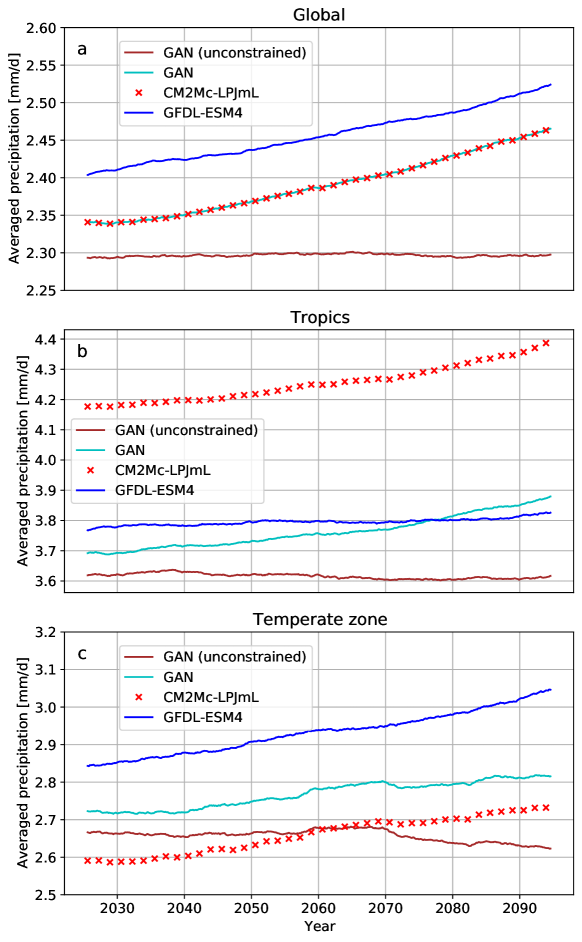
Figure 4: Large-scale trends as a three year rolling-mean of monthly and spatially average precipitation for the CMIP6 SSP5-8.5 scenario. For (a) global data, (b) the tropics and (c) temperate zone, of the CM2Mc-LPJmL (red crosses) and GFLD-ESM4 (blue) models, as well as the constrained (cyan) and unconstrained (brown) GANs. Only by adding the physical constrained to preserve the global precipitation amount per timestep enables the GAN (cyan) to follow the transient dynamics of the non-stationary climate scenario.

2.4 Interpretability of the GAN-based correction

We investigate in the following whether the GAN has learned an ESM output correction that is also physically reasonable. The attribution maps are computed with SmoothGrad for each prediction of the discriminator $D_{Y}$, with daily CM2Mc-LPJmL precipitation fields given as input. The discriminator has been trained to distinguish between reanalysis (ERA5) and GAN-processed precipitation fields and we are interested to see which spatial regions in the ESM output the discriminator regards as most important for the distinction. These regions then need to be corrected the most by the generator, implying where the most pronounced biases of CM2Mc-LPJmL are.

The temporal average of the CM2Mc-LPJmL precipitation is shown in Fig. 5 together with the absolute value of the attribution map as contour lines. The regions of highest importance are shown in red and coincide with the region in the western Pacific where the strongest biases and in particular the double-peaked ITCZ of CM2Mc-LPJmL are located (as shown in Fig. 2 and Fig. S1). Although the GAN is trained on daily precipitation fields, it has thus learned to identify regions that show biases occurring on interseasonal to interannual scales.

Figure 5: Annual average of daily precipitation fields from CM2Mc-LPJmL (color shading with scale according to the colorbar on the left) together with attribution maps (contour lines with color scale according to colorbar on the right). Note that we applied a Gaussian filter to the attribution maps to further reduce the noise. A standard deviation $\sigma=1.5$ for the filter was found to give robust results. The pacific region in the tropics shows the highest annual mean precipitation, and also the highest feature importance. The same region also exhibits the largest bias of CM2Mc-LPJmL, see in Fig. 2. Note that especially the double-ITCZ bias is a common and long-standing problem in the precipitation output of many general circulation models [Tian  Dong (2020)].

3 Discussion

We have introduced a physically constrained generative adversarial network that, combined with the computationally lightweight and efficient CM2Mc-LPJmL Earth system model, is able to produce highly realistic precipitation simulations at low computational costs.

Our method improves the ESM output in two ways: (i) the temporal distributions of the CM2Mc-LPJmL model precipitation, as well as (ii) the spatial patterns and in particular the spatial intermittency of the CM2Mc-LPJmL model precipitation. Our approach is evaluated against quantile mapping [Cannon . (2015)] and the much more advanced CMIP6 GFDL-ESM4 model, [Krasting . (2018)] taking ERA5 reanalysis data as ground truth. Note that any other, and especially purely observational, precipitation dataset with sufficient temporal resolution could readily be used instead.

Given that the training samples are unpaired as a result of the chaotic nature of observed and simulated Earth system trajectories, a comparison of single prediction-target pairs is not possible. We therefore evaluate the GAN performance on long-term summary statistics over the entire test set period. When evaluating the skill to improve temporal distributions, we find that our proposed method outperforms both baselines, showing the lowest mean errors and the smallest difference in the 95th precipitation percentile. The improvement over quantile mapping is especially pronounced for seasonal time series, where only our method successfully removes the double-peaked ITCZ of the CM2Mc-LPJmL model. This is in contrast to the results by [François . (2021)], who report a comparable skill of their CycleGAN implementation with quantile mapping for regional climate simulations. Our method corrects relative frequency histograms over the entire range of precipitation values, similarly well to QM, which is designed for this task.

Crucially, our GAN-based approach also improves the spatial structure of the ESM precipitation fields, which is not possible with traditional approaches. The GAN yields realistically intermittent spatial patterns that are characteristic for precipitation on all resolved scales, and in this regard outperforms both the quantile-mapping-based post-processing and the comprehensive, high-resolution GFDL-ESM4 model. These results show that our method, combined with the computationally lightweight and efficient CM2Mc-LPJmL ESM, can produce precipitation fields that are at least comparable to state-of-the-art, and much more computationally expensive CMIP6 models.

We applied our method to the strongly non-stationary SSP5-8.5 CMIP6 climate scenario until 2100 to test the GAN’s ability to capture these non-stationarity and the transient dynamics. The unconstrained GAN trained on observations does not generalize to the unseen climate state. It does not show an increase in global mean precipitation, as one would expect from the thermodynamic Clausius-Clapeyron relation and as seen in the numerical ESMs [Allan  Soden (2008), Donat . (2013), Guerreiro . (2018), Traxl . (2021)]. This can be explained by the fact that the precipitation of the future scenario lies well outside the training distribution. To solve this and help the GAN to generalize to this kind of out-of-sample prediction, a physical constraint to preserve the global precipitation amount of the ESM in each time step was introduced as additional network layer in the GAN. The global constraint allows the GAN to improve the precipitation regionally by accounting for local characteristics, while producing the same global mean as the ESM by construction. Conserving a physical quantity that is simulated numerically, such as the global precipitation sum in our study, also means that it cannot be improved with respect to observations by definition of the constraint. The global precipitation trend can, however, be expected to be represented comparably well in the numerical ESM through thermodynamic processes. Adding this constraint enables the GAN to follow the non-stationary, transient dynamics of the SSP5-8.5 scenario.

The generator architecture in this study is deterministic, producing the same input-output-pairs once it is trained. This enables run-to-run reproducibility, where uncertainties of the ESM can then be quantified through ensemble runs. Since the training itself is stochastic, one can create an ensemble to estimate the uncertainties resulting from GAN training (see Fig. S14). A potential direction for future research could be to develop a stochastic model that directly learns the uncertainties.

We demonstrate how feature attribution from interpretable Artifical Intelligence can be applied for a GAN, enabling a physical interpretation of this deep learning model. We find that the discriminator part of the GAN has learned to identify those regions for its decisions that are critical also from a physical perspective. These regions highlighted by our GAN interpretation are the ones with the highest absolute errors of the raw CM2Mc-LPJmL, and are known to be the most problematic for ESM precipitation in general. Namely, the tropical Pacific Ocean was found to be of highest importance for the discriminator. In this region, the particularly heavy precipitation is often caused by deep convection-driven clouds, which are difficult to model numerically [Tian  Dong (2020)]. The sensitivity of the discriminator in the Pacific region also explains the effectiveness of our generator network to reduce the double-peaked ITCZ bias. This is the region where the generator needs to modify the CM2Mc-LPJmL precipitation field most in order to avoid rejection by the discriminator. The results indicate that the GAN has successfully learned the long-term statistics while being trained on samples of much shorter time scales. This makes GANs particularly suitable for climate applications, where training samples and the statistics of interest are often on very different time scales.

The main contribution of our approach is the efficient simulations of highly realistic precipitation fields, by combining a physically constrained GAN with an ESM of reduced complexity. Producing similarly realistic fields purely numerically would require much more computational resources. For comparison, our post-processed CM2Mc-LPJmL ESM takes about 0.5 hours to compute a model year using 28 CPUs, whereas the much more complex GFDL-ESM4 requires 2 hours computational time on 1000 CPUs for a model year [Krasting . (2018)]. This corresponds to an increased computational efficiency by roughly two orders of magnitude, keeping in mind that GFDL-ESM4 produces higher resolution output. The time the GAN post-processing takes is negligible in comparison, taking 0.35 seconds per model year on a V100 GPU and 37.17 seconds on a single CPU. The quantile mapping is similarly efficient taking 0.59 seconds per model year on a CPU.

Based on our findings, there are several directions for extending our method. Down-scaling applications that increase the resolution of the ESM could be a direction for future research. Conditioning the generator by adding variables that are physically linked to precipitation, such as humidity, temperature, or wind, could further improve our method. The precipitation data, improved by our method, may be used as input to other stand-alone Earth system components such as vegetation, that require realistic climate input.

Data availability

The ERA5 reanalysis data is available for download at the Copernicus Climate Change Service (C3S) (https://cds.climate.copernicus.eu/cdsapp#!/dataset/reanalysis-era5-single-levels?tab=overview and https://cds.climate.copernicus.eu/cdsapp#!/dataset/reanalysis-era5-single-levels-preliminary-back-extension?tab=overview). Output data from the CM2Mc-LPJmL model is available at https://doi.org/10.5281/zenodo.4683086 [Drüke (2021)]. The CMIP6 data can be downloaded at https://esgf-node.llnl.gov/projects/cmip6/.

Code availability

For the CM2Mc-LPJmL model code see https://doi.org/10.5281/zenodo.4700270 [Drüke, Petri . (2021)]. The Python code for processing and analysing the data, together with the PyTorch Lightning [Falcon . (20191), Falcon . (20192)] code for training is available as a compute capsule at Code Ocean: https://doi.org/10.24433/CO.2750913.v1 [Hess . (2022)].

Competing interests

The authors declare no competing interests.

Authors contribution

PH and NB conceived the research and designed the study with input from all authors. PH performed the numerical analysis. MD conducted the CM2Mc-LPJmL experiments. All authors interpreted and discussed the results. PH wrote the manuscript with input from all authors.

Materials and Methods

The Earth system model CM2Mc-LPJmL

The coupled Earth system model CM2Mc-LPJmL v1.0 [Drüke, von Bloh . (2021)] combines the coarse-grained but relatively fast atmosphere and ocean model CM2Mc [Galbraith . (2011)] with the state-of-the-art dynamic global vegetation model (DGVM) LPJmL5 [Schaphoff . (20181), Schaphoff . (20182), Von Bloh . (2018)].

CM2Mc is a coarser (3°x3.75° latitude-longitude) configuration of the Climate Model CM2 [Milly  Shmakin (2002)], which has been developed at the Geophysical Fluid Dynamics Laboratory (GFDL). The original configuration of CM2Mc includes the Modular Ocean Model 5 (MOM5) and the global atmosphere and land models AM2-LM2 or AM2-LM [Anderson . (2004)] with static vegetation. In CM2Mc-LPJmL, the land component LM/LM2 is replaced by the dynamic global vegetation model LPJmL5, while AM2 and MOM5 remain dynamically coupled to the model framework. The Flexible Modeling System (FMS) developed by GFDL connects all different model compartments and calculates the fluxes between them.
The state-of-the-art and thoroughly validated DGVM LPJmL (Lund-Potsdam-Jena managed Land) simulates global surface energy balance, water fluxes and carbon stocks and fluxes for natural and managed land. Being forced by climate and soil data, LPJmL simulates the impact of bioclimatic limits and effects of heat, productivity and fire on plant mortality to determine the establishment, growth, competition and mortality for different plant functional types (PFTs) in natural vegetation and crop functional types (CFTs) on managed land. Since its original implementation [Sitch . (2003)] the model now incorporates a water balance [Gerten . (2004)], agriculture [Bondeau . (2007)], wildfire in natural vegetation [Thonicke . (2010), Drüke . (2019)], and the impact of multiple climate drivers on phenology [Forkel . (2014), Forkel . (2019)].

In CM2Mc-LPJmL, the fluxes simulated by LPJmL depend, of course, on the precipitation modelled by AM2. As a stand-alone model LPJmL has been mainly calibrated with respect to reanalysis, and a similarly accurate precipitation output within CM2Mc-LPJmL would hence be favorable to maintain consistency and to obtain realistic surface fluxes from LPJmL. For the overall performance of CM2Mc-LPJmL, realistically simulated precipitation fields are therefore crucial. This motivates the work presented below, where we use a specific kind of GAN to transform the AM2 precipitation fields toward fields that are indistinguishable from ERA5 precipitation fields (see below).

The model experiments of this paper are consistent with [Drüke, von Bloh . (2021)]. After a 5000-year stand-alone LPJmL spin-up, a second fully coupled spin-up under pre-industrial conditions without land use was performed for 1250 model years. In this way we ensure that the model starts from a consistent equilibrium between the long-term soil carbon pool, vegetation, ocean, and climate.

The subsequent transient historic phase of the model is performed from 1700-2018, using historic land use data from 1700 [Fader . (2010)] and historic concentrations of greenhouse gases, solar radiation, ozone concentrations and aerosols from 1860, which were kept at pre-industrial conditions beforehand.

From 2019 until 2100 the model is forced by constant land use from the year 2018 and CO₂ equivalents of the atmospheric forcing prescribed in the CMIP6 SSP5-8.5 (“business as usual”) climate scenario that assumes a continued increase in CO₂ emissions.

Cycle-consistent generative adversarial networks

Generative adversarial networks (GANs) are designed to learn a target distribution $p_{y}(y)$ through a two-player “minimax” game between a generator $G$ and a discriminator $D$ [Goodfellow . (2014)]. The generator network is trained to transform an input $x\in X$ to values that approximate samples from a target domain $y\in Y$, i.e. the generator is trained to learn the mapping $G:X\rightarrow Y$. Samples from the generator and the target dataset are then shown to the discriminator, which classifies their origin. In this way, the generator and discriminator compete against each other, thereby improving the quality of the generated samples. The training can be formulated as

$$G^{*}=\underset{G}{\mathrm{min}}\;\underset{D}{\mathrm{max}}\;\mathcal{L}_{GAN}(D,G),$$ (1)

where $G^{*}$ is the optimal generator and $\mathcal{L}_{\mathrm{GAN}}(D,G)$ is the loss function defined as

$$\mathcal{L}_{\mathrm{GAN}}(D,G)=\mathbb{E}_{y\sim p_{y}(y)}[\log(D(y))]+\mathbb{E}_{x\sim p_{x}(x)}[\log(1-D(G(x)))].$$ (2)

In our situation, $X$ and $Y$ correspond to the sets containing precipitation fields from the CM2Mc-LPJmL Earth system model and ERA5 reanalysis, respectively (samples are shown in Fig. 3). In the above formulation, GANs have often been found to suffer from instabilities and difficulties to generalize to distributions of higher dimensionality, such as in image-to-image translation without pairwise matching samples. One reason for the instabilities is the highly under-constrained mapping to be learned by the generator. To alleviate this problem, cycle-consistent GANs have been proposed recently [Zhu . (2017)]. They aim to constrain the space of mappings by training a second pair of generator and discriminator networks, which learns the inverse mapping $F:Y\rightarrow X$. A schematic of the cycle-consistent GAN model is shown in Fig. 1. Both generators should perform bijective (i.e., one-to-one) mappings [Zhu . (2017)] and are therefore trained at the same time, together with a regularization term that enforces consistency of translation cycles, i.e. $x\rightarrow G(x)\rightarrow F(G(x))\approx x$ and vice versa for $y$. The corresponding loss functions are then

$$\mathcal{L}_{X\rightarrow Y}(G,D_{Y}) =\mathbb{E}_{y\sim p_{y}(y)}[\log(D_{Y}(y))]$$ (3)

$$+\mathbb{E}_{x\sim p_{x}(x)}[\log(1-D_{Y}(G(x)))],$$

and similarly,

$$\mathcal{L}_{Y\rightarrow X}(F,D_{X}) =\mathbb{E}_{x\sim p_{x}(x)}[\log(D_{X}(x))]$$ (4)

$$+\mathbb{E}_{y\sim p_{y}(y)}[\log(1-D_{X}(F(y)))].$$

The cycle-consistency loss is given by

$$\mathcal{L}_{cycle}(G,F) =\mathbb{E}_{x\sim p_{x}(x)}[||F(G(x))-x||_{1}]$$ (5)

$$+\mathbb{E}_{y\sim p_{y}(y)}[||G(F(y))-y||_{1}].$$

The full loss function then reads

$$\mathcal{L}(G,F,D_{X},D_{Y})= \mathcal{L}_{X\rightarrow Y}(G,D_{Y})$$

$$+ \mathcal{L}_{Y\rightarrow X}(F,D_{X})$$ (6)

$$+ \lambda\mathcal{L}_{cycle}(G,F),$$

which is solved as

$$G^{*},F^{*}=\underset{G,F}{\mathrm{min}}\;\underset{D_{X},D_{Y}}{\mathrm{max}}\;\mathcal{L}(G,F,D_{X},D_{Y}).$$ (7)

We adopt the architecture from zhu2017unpaired and optimize the networks with Adam [Kingma  Ba (2014)], using a learning rate of $2e^{-4}$ for both the generator and the discriminator networks and set $\lambda=10$. Following zhu2017unpaired we set the batch size to 1 and train the models for 250 epochs, logging the 50 best performing generators every 10 epochs. The training takes about 5.25 days on a NVIDIA V100 GPU with 32 GB memory. After training the final generator is determined by evaluation on the test set.

Neural network architectures

The generator architecture is based on a variant of convolutional residual networks [He . (2016)]. Convolutional neural networks (CNNs) are commonly employed to process image data. CNNs transform the input data through stacked layers of trainable convolutional filters that are followed by a non-linear activation functions thereby learning to extract spatial patterns. For a more detailed introduction see, e.g., [Goodfellow . (2016)]. Adopting the naming convention from [Johnson . (2016), Zhu . (2017)]. c7s1-k denotes a layer with a $7\times 7$ convolution followed by instance normalization and ReLU activation with $k$ filters, a stride 1 and reflection padding. dk represents a layer with $3\times 3$ convolutions, instance normalization, ReLU activation, $k$ filters and stride 2. Rk are residual blocks with a $3\times 3$ convolutional layer and $k$ filters. uk denots a layer with $3\times 3$ fractional-strided convolutions, instance normalization, ReLU activation, $k$ filters and stride $1/2$. The generator architecture with 6 residual blocks is then

$$x_{\mathrm{in}}\rightarrow\textsf{c7s1-64}\rightarrow\textsf{d128}\rightarrow\textsf{d256}\rightarrow\underbrace{[\textsf{R256}\rightarrow]}_{\times 6}\textsf{u128}\rightarrow\textsf{u64}\rightarrow\textsf{c7s1-3}\rightarrow y_{\mathrm{out}},$$

where $x_{\mathrm{in}}$ is the input of the generator and $y_{\mathrm{out}}$ the output. The discriminator architecture is based on the PatchGAN [Isola . (2017)]. Denoting a $4\times 4$ convolutional layer with $k$ filters, instance normalization (except for the first layer), leaky ReLU with slope $0.2$ and a stride of $2$ with Ck. The full architecture of the discriminator is

$$x_{\mathrm{in}}\rightarrow\textsf{C64}\rightarrow\textsf{C128}\rightarrow\textsf{C256}\rightarrow\textsf{C512}\rightarrow y_{\mathrm{out}}.$$

Generator constraint

To enable a better generalization of the GAN to climate states not seen during training, and hence in particular to address the out-of-sample problem imposed by the changing radiative forcing due to anthropogenic greenhouse gas emissions, we introduce the physical constraint of preserving the total global precipitation amount of the CM2Mc-LPJmL model input. That is, we add an additional layer to the generator network after training, which re-scales each output $y_{i}$ at each grid point $i$ as

$$\tilde{y}_{i}=y_{i}\frac{\sum_{i}^{N_{\textrm{grid}}}x_{i}}{\sum_{i}^{N_{\textrm{grid}}}y_{i}},$$ (8)

where $N_{\textrm{grid}}$ is the total number of grid-points, $x_{i}$ the CM2Mc-LPJmL precipitation input and $\tilde{y}_{i}$ the constrained output. The motivation of the constraint is that it gives the GAN freedom to change the precipitation locally and to redistribute it in space, while forcing it to follow the global trend prescribed by the ESM. The global trend has been found to be well represented in the ESM, where noise and and biases found on small time and spatial scales are averaged out [Drüke, von Bloh . (2021)]. Also in observations, it has recently been shown that the physically based Clausius-Clapeyron relation, suggesting a 7% increase in precipitation per degree of warming, holds very well in terms of global averages, despite pronounced regional deviations [Traxl . (2021)].

Training

We use daily precipitation from the European Center for Medium-Range Weather Forecasts (ECMWF) Reanalysis v5 (ERA5) product [Hersbach . (2020)] as a training target and ground truth for evaluation. This reanalysis is produced by the Copernicus Climate Change Service (C3S) at ECMWF, combining a large range of satellite- and land-based observations with high-resolution simulations through state-of-the-art data assimilation techniques [Courtier . (1994), Hersbach . (2020)]. The original resolution is 30km horizontally in space and hourly in time, spanning the period from 1950 to present. For this study the data is aggregated to daily precipitation sums and re-gridded, following [Rasp . (2020), Beck . (2019)], by bilinear interpolation using the xESMF package [Zhuang . (2020)], in order to match the resolution of CM2Mc-LPJmL. We split the ESM and ERA5 datasets into the training period 1950-2000 and the test period 2001-2014 (for which also the GFDL-ESM4 data is available), with 18615 and 5110 daily samples, respectively. Model simulations from 2019-2100 are used to test the generalization of the network with a CO₂ forcing according the CMIP6 SSP5-8.5 (“business as usual”) climate scenario, which assumes a continued increase in CO₂ emissions. Following zhu2017unpaired, we replace the log likelihood by a least-squares loss, which has been found to improve the training. The GAN loss in Eq. 2 is then minimized by both $G$ and $D$, with a loss $\mathbb{E}_{x\sim p_{x}(x)}[(D(G(x))-1)^{2}]$ for $G$ and $\mathbb{E}_{y\sim p_{y}(y)}[(D(y)-1)^{2}]+\mathbb{E}_{x\sim p_{x}(x)}[(D(G(x)))^{2}]$ for the discriminator $D$. We apply a log-transform to the input data with $\tilde{x}=\log(x+\epsilon)-\log(\epsilon)$ following [Rasp  Thuerey (2021)], where $\tilde{x}$ is the transformed precipitation and $\epsilon=0.0001$. We further normalize the data to the interval $[-1,1]$, which was found to improve the training performance. Once trained, the generator takes only about ten seconds on a NVIDIA V100 GPU to process the test set ESM precipitation.

Baselines

We compare our method to quantile mapping, implemented with the xClim package [Logan . (2021)], and also carry out comparisons to the raw output of the more advanced CMIP6 climate model GFDL-ESM4 [Krasting . (2018)]. The latter uses AM4 [Zhao . (20181), Zhao . (20182)], a more recent and substantially more complex version of the atmosphere model AM2 used in CM2Mc-LPJmL [GFDL Global Atmospheric Model Development Team . (2004)], with a substantially higher spatial resolution and strongly improved parameterizations of subgrid-scale processes. These improvements of course come at the expense of substantially increased computational costs. The motivation here is to see whether a comparably simple atmospheric general circulation model (GCM) such as AM2 can be combined with the proposed GAN model in order to yield similar results as a comprehensive state-of-the-art atmospheric GCM such as AM4, at a fraction of the computational costs.
Quantile mapping uses the empirical cumulative distribution functions of simulated and observed precipitation to transform the simulated values into the corresponding quantiles derived from observations. Before computing the cumulative distribution function, following [Cannon . (2015)], we detrend the historical time series, assuming a linear trend.
As an error metric to compare our methods we apply the mean error (ME), which is defined as

$$\textrm{ME}=\frac{1}{N}\sum_{t=1}^{N_{time}}(x_{t}-y_{t})=\frac{1}{N}\sum_{t=1}^{N_{time}}x_{t}-\frac{1}{N}\sum_{t=1}^{N_{time}}y_{t},$$ (9)

where $x_{t}$ and $y_{t}$ are the simulated and observed precipitation at time $t$ for a given grid cell and $N_{time}$ the number of time steps in the test set. Note that the ME is used to evaluate the differences in the time averages per grid cell, as can be seen on the right-hand side of Eq. 9.

Model transparency

Neural network models are often regarded as black boxes. Since it is important for many applications to be able to explain the neural network’s prediction, the emergent fields of interpretable [Murdoch . (2019), Toms . (2020)] and explainable Artificial Intelligence [Sundararajan . (2017), Montavon . (2019)] aim to improve the transparency.

Many methods for interpreting neural networks are specifically designed for classification problems [Goodfellow . (2016)]. In the GAN framework, the discriminator network performs such a classification task in distinguishing between generated and real images. Hence, suitable interpretability methods can be applied, even though entire GAN is build for the much more complex generative task. Being able to interpret the GAN increases the transparency and trust, since it ensures that the model has learned to identify physically reasonable input features. To our knowledge, we are the first to apply an interpretability method in such a way, i.e., to test the physical consistency of the GAN training.

Here, we use the gradient-based method SmoothGrad [Smilkov . (2017)] to interpret the discriminator network $D_{Y}$ that has learned to classify ERA5 and generated precipitation fields. An attribution map $\phi$ is computed by taking the gradient of the neural network $D_{Y}$ with respect to its input $y$,

$$\phi(D_{Y},y)=\frac{\partial D_{Y}(y)}{\partial y},$$ (10)

showing for each input grid cell how much the prediction will change with respect to its input, i.e. how sensitive it is to perturbations of the input. It has been observed that using only the gradient of the input, however, tends to give rather noisy attribution maps. Therefore, smilkov2017smoothgrad proposed a technique to reduce the noise, by adding it to the network’s input and averaging the gradient over a sample size, e.g. here $N=10$, as

$$\hat{\phi}(D_{Y},y)=\frac{1}{N}\sum^{N}_{i=1}\phi\left(y+\epsilon_{i}\right),$$ (11)

where the noise is sampled from a Gaussian distribution $\epsilon_{i}\sim\mathcal{N}\left(0,\sigma^{2}\right)$.

References

- Allan \BBA Soden (\APACyear2008) \APACinsertmetastarallan2008atmospheric{APACrefauthors}Allan, R\BPBIP.\BCBT \BBA Soden, B\BPBIJ. \APACrefYearMonthDay2008. \BBOQ\APACrefatitleAtmospheric warming and the amplification of precipitation extremes Atmospheric warming and the amplification of precipitation extremes.\BBCQ \APACjournalVolNumPagesScience32158951481–1484. \PrintBackRefs\CurrentBib
- Anderson \BOthers. (\APACyear2004) \APACinsertmetastarAnderson2004TheSimulations{APACrefauthors}Anderson, J\BPBIL., Balaji, V., Broccoli, A\BPBIJ., Cooke, W\BPBIF., Delworth, T\BPBIL., Dixon, K\BPBIW.\BDBLWyman, B\BPBIL. \APACrefYearMonthDay2004. \BBOQ\APACrefatitleThe new GFDL global atmosphere and land model AM2-LM2: Evaluation with prescribed SST simulations The new GFDL global atmosphere and land model AM2-LM2: Evaluation with prescribed SST simulations.\BBCQ \APACjournalVolNumPagesJournal of Climate17244641–4673. {APACrefDOI} 10.1175/JCLI-3223.1 \PrintBackRefs\CurrentBib
- Beck \BOthers. (\APACyear2019) \APACinsertmetastarbeck2019mswep{APACrefauthors}Beck, H\BPBIE., Wood, E\BPBIF., Pan, M., Fisher, C\BPBIK., Miralles, D\BPBIG., Van Dijk, A\BPBII.\BDBLAdler, R\BPBIF. \APACrefYearMonthDay2019. \BBOQ\APACrefatitleMSWEP V2 global 3-hourly 0.1 precipitation: methodology and quantitative assessment MSWEP V2 global 3-hourly 0.1 precipitation: methodology and quantitative assessment.\BBCQ \APACjournalVolNumPagesBulletin of the American Meteorological Society1003473–500. {APACrefDOI} 10.1175/BAMS-D-17-0138.1 \PrintBackRefs\CurrentBib
- Beucler \BOthers. (\APACyear2021) \APACinsertmetastarbeucler2021enforcing{APACrefauthors}Beucler, T., Pritchard, M., Rasp, S., Ott, J., Baldi, P.\BCBL \BBA Gentine, P. \APACrefYearMonthDay2021. \BBOQ\APACrefatitleEnforcing analytic constraints in neural networks emulating physical systems Enforcing analytic constraints in neural networks emulating physical systems.\BBCQ \APACjournalVolNumPagesPhysical Review Letters1269098302. \PrintBackRefs\CurrentBib
- Bondeau \BOthers. (\APACyear2007) \APACinsertmetastarBondeau2007Mar{APACrefauthors}Bondeau, A., Smith, P\BPBIC., Zaehle, S., Schaphoff, S., Lucht, W., Cramer, W.\BDBLSmith, B. \APACrefYearMonthDay2007. \BBOQ\APACrefatitleModelling the role of agriculture for the 20th century global terrestrial carbon balance Modelling the role of agriculture for the 20th century global terrestrial carbon balance.\BBCQ \APACjournalVolNumPagesGlobal Change Biol.133679–706. {APACrefDOI} 10.1111/j.1365-2486.2006.01305.x \PrintBackRefs\CurrentBib
- Boyle \BBA Klein (\APACyear2010) \APACinsertmetastarboyle2010impact{APACrefauthors}Boyle, J.\BCBT \BBA Klein, S\BPBIA. \APACrefYearMonthDay2010. \BBOQ\APACrefatitleImpact of horizontal resolution on climate model forecasts of tropical precipitation and diabatic heating for the TWP-ICE period Impact of horizontal resolution on climate model forecasts of tropical precipitation and diabatic heating for the TWP-ICE period.\BBCQ \APACjournalVolNumPagesJournal of Geophysical Research: Atmospheres115D23. {APACrefDOI} 10.1029/2010JD014262 \PrintBackRefs\CurrentBib
- Cannon \BOthers. (\APACyear2015) \APACinsertmetastarcannon2015bias{APACrefauthors}Cannon, A\BPBIJ., Sobie, S\BPBIR.\BCBL \BBA Murdock, T\BPBIQ. \APACrefYearMonthDay2015. \BBOQ\APACrefatitleBias correction of GCM precipitation by quantile mapping: How well do methods preserve changes in quantiles and extremes? Bias correction of GCM precipitation by quantile mapping: How well do methods preserve changes in quantiles and extremes?\BBCQ \APACjournalVolNumPagesJournal of Climate28176938–6959. {APACrefDOI} 10.1175/JCLI-D-14-00754.1 \PrintBackRefs\CurrentBib
- Courtier \BOthers. (\APACyear1994) \APACinsertmetastarcourtier1994strategy{APACrefauthors}Courtier, P., Thépaut, J\BHBIN.\BCBL \BBA Hollingsworth, A. \APACrefYearMonthDay1994. \BBOQ\APACrefatitleA strategy for operational implementation of 4D-Var, using an incremental approach A strategy for operational implementation of 4D-Var, using an incremental approach.\BBCQ \APACjournalVolNumPagesQuarterly Journal of the Royal Meteorological Society1205191367–1387. \PrintBackRefs\CurrentBib
- Déqué (\APACyear2007) \APACinsertmetastardeque2007frequency{APACrefauthors}Déqué, M. \APACrefYearMonthDay2007. \BBOQ\APACrefatitleFrequency of precipitation and temperature extremes over France in an anthropogenic scenario: Model results and statistical correction according to observed values Frequency of precipitation and temperature extremes over France in an anthropogenic scenario: Model results and statistical correction according to observed values.\BBCQ \APACjournalVolNumPagesGlobal and Planetary Change571-216–26. \PrintBackRefs\CurrentBib
- Donat \BOthers. (\APACyear2013) \APACinsertmetastardonat2013updated{APACrefauthors}Donat, M\BPBIG., Alexander, L\BPBIV., Yang, H., Durre, I., Vose, R., Dunn, R\BPBIJ\BPBIH.\BDBLKitching, S. \APACrefYearMonthDay2013. \BBOQ\APACrefatitleUpdated analyses of temperature and precipitation extreme indices since the beginning of the twentieth century: The HadEX2 dataset Updated analyses of temperature and precipitation extreme indices since the beginning of the twentieth century: The HadEX2 dataset.\BBCQ \APACjournalVolNumPagesJournal of Geophysical Research: Atmospheres11852098–2118. {APACrefDOI} 10.1002/jgrd.50150 \PrintBackRefs\CurrentBib
- Drüke (\APACyear2021) \APACinsertmetastardata-gmd-2020-436{APACrefauthors}Drüke, M. \APACrefYearMonthDay2021\APACmonth04. \APACrefbtitleOutput data for the GMD publication gmd-2020-436. Output data for the GMD publication gmd-2020-436. \APAChowpublished[Data set] Zenodo. {APACrefDOI} 10.5281/zenodo.4683086 \PrintBackRefs\CurrentBib
- Drüke \BOthers. (\APACyear2019) \APACinsertmetastarDruke2019ImprovingData{APACrefauthors}Drüke, M., Forkel, M., von Bloh, W., Sakschewski, B., Cardoso, M., Bustamante, M.\BDBLThonicke, K. \APACrefYearMonthDay2019. \BBOQ\APACrefatitleImproving the LPJmL4-SPITFIRE vegetation-fire model for South America using satellite data Improving the LPJmL4-SPITFIRE vegetation-fire model for South America using satellite data.\BBCQ \APACjournalVolNumPagesGeoscientific Model Development12125029–-5054. {APACrefDOI} 10.5194/gmd-12-5029-2019 \PrintBackRefs\CurrentBib
- Drüke, Petri\BCBL \BOthers. (\APACyear2021) \APACinsertmetastarcode-gmd-2020-436{APACrefauthors}Drüke, M., Petri, S., von Bloh, W.\BCBL \BBA Schaphoff, S. \APACrefYearMonthDay2021\APACmonth04. \APACrefbtitleModel code for the GMD publication gmd-2020-436 (Version 1.0). Model code for the GMD publication gmd-2020-436 (Version 1.0). \APAChowpublished[Data set] Zenodo. {APACrefDOI} 10.5281/zenodo.4700270 \PrintBackRefs\CurrentBib
- Drüke, von Bloh\BCBL \BOthers. (\APACyear2021) \APACinsertmetastardruke2021cm2mc{APACrefauthors}Drüke, M., von Bloh, W., Petri, S., Sakschewski, B., Schaphoff, S., Forkel, M.\BDBLThonicke, K. \APACrefYearMonthDay2021. \BBOQ\APACrefatitleCM2Mc-LPJmL v1.0: Biophysical coupling of a process-based dynamic vegetation model with managed land to a general circulation model CM2Mc-LPJmL v1.0: Biophysical coupling of a process-based dynamic vegetation model with managed land to a general circulation model.\BBCQ \APACjournalVolNumPagesGeoscientific Model Development1464117–4141. {APACrefDOI} 10.5194/gmd-14-4117-2021 \PrintBackRefs\CurrentBib
- Fader \BOthers. (\APACyear2010) \APACinsertmetastarFader2010Apr{APACrefauthors}Fader, M., Rost, S., Mueller, C., Bondeau, A.\BCBL \BBA Gerten, D. \APACrefYearMonthDay20104. \BBOQ\APACrefatitleVirtual water content of temperate cereals and maize: Present and potential future patterns Virtual water content of temperate cereals and maize: Present and potential future patterns.\BBCQ \APACjournalVolNumPagesJ. Hydrol.3843218–231. {APACrefDOI} 10.1016/j.jhydrol.2009.12.011 \PrintBackRefs\CurrentBib
- Falcon \BOthers. (\APACyear2019\APACexlab\BCnt1) \APACinsertmetastarfalcon2019pytorch{APACrefauthors}Falcon, W.\BCBT \BOthersPeriod. \APACrefYearMonthDay2019\BCnt1. \BBOQ\APACrefatitlePytorch lightning Pytorch lightning.\BBCQ \APACjournalVolNumPagesGitHub. Note: https://github.com/PyTorchLightning/pytorch-lightning36. \PrintBackRefs\CurrentBib
- Falcon \BOthers. (\APACyear2019\APACexlab\BCnt2) \APACinsertmetastarpytorch2019{APACrefauthors}Falcon, W.\BCBT \BOthersPeriod. \APACrefYearMonthDay2019\BCnt2. \APACrefbtitlePyTorch Lightning. PyTorch Lightning. \APAChowpublishedGitHub repository. {APACrefURL} https://github.com/PyTorchLightning/pytorch-lightning \PrintBackRefs\CurrentBib
- Forkel \BOthers. (\APACyear2014) \APACinsertmetastarForkel2014IdentifyingIntegration{APACrefauthors}Forkel, M., Carvalhais, N., Schaphoff, S., von Bloh, W., Migliavacca, M., Thurner, M.\BCBL \BBA Thonicke, K. \APACrefYearMonthDay2014. \BBOQ\APACrefatitleIdentifying environmental controls on vegetation greenness phenology through model-data integration Identifying environmental controls on vegetation greenness phenology through model-data integration.\BBCQ \APACjournalVolNumPagesBiogeosciences11237025–7050. {APACrefDOI} 10.5194/bg-11-7025-2014 \PrintBackRefs\CurrentBib
- Forkel \BOthers. (\APACyear2019) \APACinsertmetastarForkel2019ConstrainingObservations{APACrefauthors}Forkel, M., Drüke, M., Thurner, M., Dorigo, W., Schaphoff, S., Thonicke, K.\BDBLCarvalhais, N. \APACrefYearMonthDay2019. \BBOQ\APACrefatitleConstraining modelled global vegetation dynamics and carbon turnover using multiple satellite observations Constraining modelled global vegetation dynamics and carbon turnover using multiple satellite observations.\BBCQ \APACjournalVolNumPagesScientific Reports91. {APACrefDOI} 10.1038/s41598-019-55187-7 \PrintBackRefs\CurrentBib
- François \BOthers. (\APACyear2021) \APACinsertmetastarfranccois2021adjusting{APACrefauthors}François, B., Thao, S.\BCBL \BBA Vrac, M. \APACrefYearMonthDay2021. \BBOQ\APACrefatitleAdjusting spatial dependence of climate model outputs with cycle-consistent adversarial networks Adjusting spatial dependence of climate model outputs with cycle-consistent adversarial networks.\BBCQ \APACjournalVolNumPagesClimate Dynamics57113323–3353. \PrintBackRefs\CurrentBib
- Gagne \BOthers. (\APACyear2020) \APACinsertmetastargagne2020machine{APACrefauthors}Gagne, D\BPBIJ., Christensen, H\BPBIM., Subramanian, A\BPBIC.\BCBL \BBA Monahan, A\BPBIH. \APACrefYearMonthDay2020. \BBOQ\APACrefatitleMachine learning for stochastic parameterization: Generative adversarial networks in the Lorenz’96 model Machine learning for stochastic parameterization: Generative adversarial networks in the Lorenz’96 model.\BBCQ \APACjournalVolNumPagesJournal of Advances in Modeling Earth Systems123e2019MS001896. \PrintBackRefs\CurrentBib
- Galbraith \BOthers. (\APACyear2011) \APACinsertmetastarGalbraith2011ClimateModel{APACrefauthors}Galbraith, E\BPBID., Kwon, E\BPBIY., Gnanadesikan, A., Rodgers, K\BPBIB., Griffies, S\BPBIM., Bianchi, D.\BDBLHeld, I\BPBIM. \APACrefYearMonthDay2011. \BBOQ\APACrefatitleClimate variability and radiocarbon in the CM2Mc earth system model Climate variability and radiocarbon in the CM2Mc earth system model.\BBCQ \APACjournalVolNumPagesJournal of Climate24164230–4254. {APACrefDOI} 10.1175/2011JCLI3919.1 \PrintBackRefs\CurrentBib
- Gerten \BOthers. (\APACyear2004) \APACinsertmetastarGerten2004Jan{APACrefauthors}Gerten, D., Schaphoff, S., Haberlandt, U., Lucht, W.\BCBL \BBA Sitch, S. \APACrefYearMonthDay20041. \BBOQ\APACrefatitleTerrestrial vegetation and water balance - hydrological evaluation of a dynamic global vegetation model Terrestrial vegetation and water balance - hydrological evaluation of a dynamic global vegetation model.\BBCQ \APACjournalVolNumPagesJ. Hydrol.2861249–270. {APACrefDOI} 10.1016/j.jhydrol.2003.09.029 \PrintBackRefs\CurrentBib
- GFDL Global Atmospheric Model Development Team \BOthers. (\APACyear2004) \APACinsertmetastargfdl2004new{APACrefauthors}GFDL Global Atmospheric Model Development Team, Anderson, J\BPBIL., Balaji, V., Broccoli, A\BPBIJ., Cooke, W\BPBIF., Delworth, T\BPBIL.\BDBLWyman, B. \APACrefYearMonthDay2004. \BBOQ\APACrefatitleThe new GFDL global atmosphere and land model AM2–LM2: Evaluation with prescribed SST simulations The new GFDL global atmosphere and land model AM2–LM2: Evaluation with prescribed SST simulations.\BBCQ \APACjournalVolNumPagesJournal of Climate17244641–4673. {APACrefDOI} 10.1175/JCLI-3223.1 \PrintBackRefs\CurrentBib
- Goodfellow \BOthers. (\APACyear2016) \APACinsertmetastargoodfellow2016deep{APACrefauthors}Goodfellow, I., Bengio, Y.\BCBL \BBA Courville, A. \APACrefYear2016. \APACrefbtitleDeep learning Deep learning. \APACaddressPublisherMIT press. \PrintBackRefs\CurrentBib
- Goodfellow \BOthers. (\APACyear2014) \APACinsertmetastargoodfellow2014generative{APACrefauthors}Goodfellow, I., Pouget-Abadie, J., Mirza, M., Xu, B., Warde-Farley, D., Ozair, S.\BDBLBengio, Y. \APACrefYearMonthDay2014. \BBOQ\APACrefatitleGenerative adversarial nets Generative adversarial nets.\BBCQ \APACjournalVolNumPagesAdvances in neural information processing systems27. \PrintBackRefs\CurrentBib
- Grönquist \BOthers. (\APACyear2021) \APACinsertmetastargronquist2021deep{APACrefauthors}Grönquist, P., Yao, C., Ben-Nun, T., Dryden, N., Dueben, P., Li, S.\BCBL \BBA Hoefler, T. \APACrefYearMonthDay2021. \BBOQ\APACrefatitleDeep learning for post-processing ensemble weather forecasts Deep learning for post-processing ensemble weather forecasts.\BBCQ \APACjournalVolNumPagesPhilosophical Transactions of the Royal Society A379219420200092. {APACrefDOI} 10.1098/rsta.2020.0092 \PrintBackRefs\CurrentBib
- Gudmundsson \BOthers. (\APACyear2012) \APACinsertmetastargudmundsson2012downscaling{APACrefauthors}Gudmundsson, L., Bremnes, J\BPBIB., Haugen, J\BPBIE.\BCBL \BBA Engen-Skaugen, T. \APACrefYearMonthDay2012. \BBOQ\APACrefatitleDownscaling RCM precipitation to the station scale using statistical transformations–a comparison of methods Downscaling RCM precipitation to the station scale using statistical transformations–a comparison of methods.\BBCQ \APACjournalVolNumPagesHydrology and Earth System Sciences1693383–3390. \PrintBackRefs\CurrentBib
- Guerreiro \BOthers. (\APACyear2018) \APACinsertmetastarguerreiro2018detection{APACrefauthors}Guerreiro, S\BPBIB., Fowler, H\BPBIJ., Barbero, R., Westra, S., Lenderink, G., Blenkinsop, S.\BDBLLi, X\BHBIF. \APACrefYearMonthDay2018. \BBOQ\APACrefatitleDetection of continental-scale intensification of hourly rainfall extremes Detection of continental-scale intensification of hourly rainfall extremes.\BBCQ \APACjournalVolNumPagesNature Climate Change89803–807. \PrintBackRefs\CurrentBib
- D. Harris \BOthers. (\APACyear2001) \APACinsertmetastarharris2001multiscale{APACrefauthors}Harris, D., Foufoula-Georgiou, E., Droegemeier, K\BPBIK.\BCBL \BBA Levit, J\BPBIJ. \APACrefYearMonthDay2001. \BBOQ\APACrefatitleMultiscale statistical properties of a high-resolution precipitation forecast Multiscale statistical properties of a high-resolution precipitation forecast.\BBCQ \APACjournalVolNumPagesJournal of Hydrometeorology24406–418. \PrintBackRefs\CurrentBib
- L. Harris \BOthers. (\APACyear2022) \APACinsertmetastarharris2022generative{APACrefauthors}Harris, L., McRae, A\BPBIT., Chantry, M., Dueben, P\BPBID.\BCBL \BBA Palmer, T\BPBIN. \APACrefYearMonthDay2022. \BBOQ\APACrefatitleA Generative Deep Learning Approach to Stochastic Downscaling of Precipitation Forecasts A generative deep learning approach to stochastic downscaling of precipitation forecasts.\BBCQ \APACjournalVolNumPagesarXiv preprint arXiv:2204.02028. \PrintBackRefs\CurrentBib
- He \BOthers. (\APACyear2016) \APACinsertmetastarhe2016identity{APACrefauthors}He, K., Zhang, X., Ren, S.\BCBL \BBA Sun, J. \APACrefYearMonthDay2016. \BBOQ\APACrefatitleIdentity mappings in deep residual networks Identity mappings in deep residual networks.\BBCQ \BIn \APACrefbtitleComputer Vision – ECCV 2016, Proceedings, Part IV Computer Vision – ECCV 2016, Proceedings, Part IV (\BPGS 630–645). \APACaddressPublisherSpringer. {APACrefDOI} 10.1007/978-3-319-46493-0_38 \PrintBackRefs\CurrentBib
- Hersbach \BOthers. (\APACyear2020) \APACinsertmetastarhersbach2020era5{APACrefauthors}Hersbach, H., Bell, B., Berrisford, P., Hirahara, S., Horányi, A., Muñoz-Sabater, J.\BDBLThépaut, J\BHBIN. \APACrefYearMonthDay2020. \BBOQ\APACrefatitleThe ERA5 global reanalysis The ERA5 global reanalysis.\BBCQ \APACjournalVolNumPagesQuarterly Journal of the Royal Meteorological Society1467301999–2049. {APACrefDOI} 10.1002/qj.3803 \PrintBackRefs\CurrentBib
- Hess \BOthers. (\APACyear2022) \APACinsertmetastarPhys_compute_capsule{APACrefauthors}Hess, P., Drüke, M., Petri, S., Strnad, F.\BCBL \BBA Boers, N. \APACrefYearMonthDay20225. \APACrefbtitlePhysically Constrained Generative Adversarial Networks for Improving Precipitation Fields from Earth System Models. Physically constrained generative adversarial networks for improving precipitation fields from earth system models. \APAChowpublishedhttps://www.codeocean.com/. {APACrefDOI} 10.24433/CO.2750913.v1 \PrintBackRefs\CurrentBib
- Hoffman \BOthers. (\APACyear2018) \APACinsertmetastarhoffman2018cycada{APACrefauthors}Hoffman, J., Tzeng, E., Park, T., Zhu, J\BHBIY., Isola, P., Saenko, K.\BDBLDarrell, T. \APACrefYearMonthDay2018. \BBOQ\APACrefatitleCycada: Cycle-consistent adversarial domain adaptation Cycada: Cycle-consistent adversarial domain adaptation.\BBCQ \BIn \APACrefbtitleInternational conference on machine learning International conference on machine learning (\BPGS 1989–1998). \PrintBackRefs\CurrentBib
- IPCC (\APACyear2021) \APACinsertmetastaripcc-ar6-wg1-2021{APACrefauthors}IPCC. \APACrefYear2021. \APACrefbtitleClimate Change 2021: The Physical Science Basis. Contribution of Working Group I to the Sixth Assessment Report of the Intergovernmental Panel on Climate Change Climate Change 2021: The Physical Science Basis. Contribution of Working Group I to the Sixth Assessment Report of the Intergovernmental Panel on Climate Change (V. Masson-Delmotte \BOthers., \BEDS). \APACaddressPublisherCambridge University Press. {APACrefURL} https://www.ipcc.ch/report/sixth-assessment-report-working-group-i/ \APACrefnoteIn Press \PrintBackRefs\CurrentBib
- Isola \BOthers. (\APACyear2017) \APACinsertmetastarIsola2017{APACrefauthors}Isola, P., Zhu, J\BPBIY., Zhou, T.\BCBL \BBA Efros, A\BPBIA. \APACrefYearMonthDay2017. \BBOQ\APACrefatitleImage-to-image translation with conditional adversarial networks Image-to-image translation with conditional adversarial networks.\BBCQ \BIn \APACrefbtitleProceedings – 30th IEEE Conference on Computer Vision and Pattern Recognition, CVPR 2017 Proceedings – 30th IEEE Conference on Computer Vision and Pattern Recognition, CVPR 2017 (\BPGS 5967–5976). {APACrefDOI} 10.1109/CVPR.2017.632 \PrintBackRefs\CurrentBib
- Johnson \BOthers. (\APACyear2016) \APACinsertmetastarjohnson2016perceptual{APACrefauthors}Johnson, J., Alahi, A.\BCBL \BBA Fei-Fei, L. \APACrefYearMonthDay2016. \BBOQ\APACrefatitlePerceptual losses for real-time style transfer and super-resolution Perceptual losses for real-time style transfer and super-resolution.\BBCQ \BIn \APACrefbtitleComputer Vision – ECCV 2016, Proceedings, Part II Computer Vision – ECCV 2016, Proceedings, Part II (\BPGS 694–711). \APACaddressPublisherSpringer. {APACrefDOI} 10.1007/978-3-319-46475-6_43 \PrintBackRefs\CurrentBib
- Kingma \BBA Ba (\APACyear2014) \APACinsertmetastarkingma2014adam{APACrefauthors}Kingma, D\BPBIP.\BCBT \BBA Ba, J. \APACrefYearMonthDay2014. \BBOQ\APACrefatitleAdam: A method for stochastic optimization Adam: A method for stochastic optimization.\BBCQ \APACjournalVolNumPagesarXiv preprint arXiv:1412.6980. \PrintBackRefs\CurrentBib
- Krasting \BOthers. (\APACyear2018) \APACinsertmetastargfdlesm4{APACrefauthors}Krasting, J\BPBIP., John, J\BPBIG., Blanton, C., McHugh, C., Nikonov, S., Radhakrishnan, A.\BDBLZhao, M. \APACrefYearMonthDay2018. \APACrefbtitleNOAA-GFDL GFDL-ESM4 model output prepared for CMIP6 CMIP. NOAA-GFDL GFDL-ESM4 model output prepared for CMIP6 CMIP. \APACaddressPublisherEarth System Grid Federation. {APACrefDOI} 10.22033/ESGF/CMIP6.1407 \PrintBackRefs\CurrentBib
- LeCun \BOthers. (\APACyear2015) \APACinsertmetastarlecun2015deep{APACrefauthors}LeCun, Y., Bengio, Y.\BCBL \BBA Hinton, G. \APACrefYearMonthDay2015. \BBOQ\APACrefatitleDeep learning Deep learning.\BBCQ \APACjournalVolNumPagesNature5217553436–444. \PrintBackRefs\CurrentBib
- Logan \BOthers. (\APACyear2021) \APACinsertmetastarlogan_travis_2021_5649661{APACrefauthors}Logan, T., Bourgault, P., Smith, T\BPBIJ., Huard, D., Biner, S., Labonté, M\BHBIP.\BDBLLavoie, J. \APACrefYearMonthDay2021\APACmonth11. \APACrefbtitleOuranosinc/xclim: v0.31.0. Ouranosinc/xclim: v0.31.0. \APACaddressPublisherZenodo. {APACrefURL} https://doi.org/10.5281/zenodo.5649661 {APACrefDOI} 10.5281/zenodo.5649661 \PrintBackRefs\CurrentBib
- Milly \BBA Shmakin (\APACyear2002) \APACinsertmetastarMilly2002GlobalModel{APACrefauthors}Milly, P\BPBIC.\BCBT \BBA Shmakin, A\BPBIB. \APACrefYearMonthDay2002. \BBOQ\APACrefatitleGlobal modeling of land water and energy balances. Part I: The land dynamics (LaD) model Global modeling of land water and energy balances. Part I: The land dynamics (LaD) model.\BBCQ \APACjournalVolNumPagesJournal of Hydrometeorology33283–299. {APACrefDOI} 10.1175/1525-7541(2002)003¡0283:GMOLWA¿2.0.CO;2 \PrintBackRefs\CurrentBib
- Mirza \BBA Osindero (\APACyear2014) \APACinsertmetastarmirza2014conditional{APACrefauthors}Mirza, M.\BCBT \BBA Osindero, S. \APACrefYearMonthDay2014. \BBOQ\APACrefatitleConditional generative adversarial nets Conditional generative adversarial nets.\BBCQ \APACjournalVolNumPagesarXiv preprint arXiv:1411.1784. \PrintBackRefs\CurrentBib
- Montavon \BOthers. (\APACyear2019) \APACinsertmetastarmontavon2019layer{APACrefauthors}Montavon, G., Binder, A., Lapuschkin, S., Samek, W.\BCBL \BBA Müller, K\BHBIR. \APACrefYearMonthDay2019. \BBOQ\APACrefatitleLayer-wise relevance propagation: an overview Layer-wise relevance propagation: an overview.\BBCQ \APACjournalVolNumPagesExplainable AI: interpreting, explaining and visualizing deep learning193–209. \PrintBackRefs\CurrentBib
- Murdoch \BOthers. (\APACyear2019) \APACinsertmetastarmurdoch2019interpretable{APACrefauthors}Murdoch, W\BPBIJ., Singh, C., Kumbier, K., Abbasi-Asl, R.\BCBL \BBA Yu, B. \APACrefYearMonthDay2019. \BBOQ\APACrefatitleInterpretable machine learning: definitions, methods, and applications Interpretable machine learning: definitions, methods, and applications.\BBCQ \APACjournalVolNumPagesarXiv preprint arXiv:1901.04592. \PrintBackRefs\CurrentBib
- Palmer \BBA Stevens (\APACyear2019) \APACinsertmetastarpalmer2019scientific{APACrefauthors}Palmer, T.\BCBT \BBA Stevens, B. \APACrefYearMonthDay2019. \BBOQ\APACrefatitleThe scientific challenge of understanding and estimating climate change The scientific challenge of understanding and estimating climate change.\BBCQ \APACjournalVolNumPagesProceedings of the National Academy of Sciences1164924390–24395. \PrintBackRefs\CurrentBib
- Price \BBA Rasp (\APACyear2022) \APACinsertmetastarprice2022increasing{APACrefauthors}Price, I.\BCBT \BBA Rasp, S. \APACrefYearMonthDay2022. \BBOQ\APACrefatitleIncreasing the accuracy and resolution of precipitation forecasts using deep generative models Increasing the accuracy and resolution of precipitation forecasts using deep generative models.\BBCQ \BIn \APACrefbtitleInternational Conference on Artificial Intelligence and Statistics International conference on artificial intelligence and statistics (\BPGS 10555–10571). \PrintBackRefs\CurrentBib
- Raissi \BOthers. (\APACyear2019) \APACinsertmetastarraissi_physics-informed_2019-2{APACrefauthors}Raissi, M., Perdikaris, P.\BCBL \BBA Karniadakis, G\BPBIE. \APACrefYearMonthDay2019\APACmonth02. \BBOQ\APACrefatitlePhysics-informed neural networks: A deep learning framework for solving forward and inverse problems involving nonlinear partial differential equations Physics-informed neural networks: A deep learning framework for solving forward and inverse problems involving nonlinear partial differential equations.\BBCQ \APACjournalVolNumPagesJournal of Computational Physics378686–707. {APACrefDOI} 10.1016/j.jcp.2018.10.045 \PrintBackRefs\CurrentBib
- Rasp \BOthers. (\APACyear2020) \APACinsertmetastarrasp2020weatherbench{APACrefauthors}Rasp, S., Dueben, P\BPBID., Scher, S., Weyn, J\BPBIA., Mouatadid, S.\BCBL \BBA Thuerey, N. \APACrefYearMonthDay2020. \BBOQ\APACrefatitleWeatherBench: a benchmark data set for data-driven weather forecasting WeatherBench: a benchmark data set for data-driven weather forecasting.\BBCQ \APACjournalVolNumPagesJournal of Advances in Modeling Earth Systems1211e2020MS002203. \PrintBackRefs\CurrentBib
- Rasp \BBA Lerch (\APACyear2018) \APACinsertmetastarrasp2018neural{APACrefauthors}Rasp, S.\BCBT \BBA Lerch, S. \APACrefYearMonthDay2018. \BBOQ\APACrefatitleNeural networks for postprocessing ensemble weather forecasts Neural networks for postprocessing ensemble weather forecasts.\BBCQ \APACjournalVolNumPagesMonthly Weather Review146113885–3900. \PrintBackRefs\CurrentBib
- Rasp \BBA Thuerey (\APACyear2021) \APACinsertmetastarrasp2021data{APACrefauthors}Rasp, S.\BCBT \BBA Thuerey, N. \APACrefYearMonthDay2021. \BBOQ\APACrefatitleData-driven medium-range weather prediction with a resnet pretrained on climate simulations: A new model for weatherbench Data-driven medium-range weather prediction with a resnet pretrained on climate simulations: A new model for weatherbench.\BBCQ \APACjournalVolNumPagesJournal of Advances in Modeling Earth Systems132e2020MS002405. \PrintBackRefs\CurrentBib
- Ravuri \BOthers. (\APACyear2021) \APACinsertmetastarravuri2021skillful{APACrefauthors}Ravuri, S., Lenc, K., Willson, M., Kangin, D., Lam, R., Mirowski, P.\BDBLMohamed, S. \APACrefYearMonthDay2021. \BBOQ\APACrefatitleSkillful Precipitation Nowcasting using Deep Generative Models of Radar Skillful precipitation nowcasting using deep generative models of radar.\BBCQ \APACjournalVolNumPagesNature597672–677. {APACrefDOI} 10.1038/s41586-021-03854-z \PrintBackRefs\CurrentBib
- Schaphoff \BOthers. (\APACyear2018\APACexlab\BCnt1) \APACinsertmetastarSchaphoff2018LPJmL4Description{APACrefauthors}Schaphoff, S., Forkel, M., Müller, C., Knauer, J., von Bloh, W., Gerten, D.\BDBLWaha, K. \APACrefYearMonthDay2018\BCnt1. \BBOQ\APACrefatitleLPJmL4 - a dynamic global vegetation model with managed land - Part 1: Model description LPJmL4 - a dynamic global vegetation model with managed land - Part 1: Model description.\BBCQ \APACjournalVolNumPagesGeoscientific Model Development1141343–1375. {APACrefDOI} 10.5194/gmd-11-1343-2018 \PrintBackRefs\CurrentBib
- Schaphoff \BOthers. (\APACyear2018\APACexlab\BCnt2) \APACinsertmetastarSchaphoff2018LPJmL4Evaluation{APACrefauthors}Schaphoff, S., Forkel, M., Müller, C., Knauer, J., von Bloh, W., Gerten, D.\BDBLWaha, K. \APACrefYearMonthDay2018\BCnt2. \BBOQ\APACrefatitleLPJmL4 - a dynamic global vegetation model with managed land: Part 2: Model evaluation LPJmL4 - a dynamic global vegetation model with managed land: Part 2: Model evaluation.\BBCQ \APACjournalVolNumPagesGeoscientific Model Development111377–1403. {APACrefDOI} 10.5194/gmd-2017-146 \PrintBackRefs\CurrentBib
- Sinclair \BBA Pegram (\APACyear2005) \APACinsertmetastarsinclair2005empirical{APACrefauthors}Sinclair, S.\BCBT \BBA Pegram, G. \APACrefYearMonthDay2005. \BBOQ\APACrefatitleEmpirical Mode Decomposition in 2-D space and time: a tool for space-time rainfall analysis and nowcasting Empirical mode decomposition in 2-D space and time: a tool for space-time rainfall analysis and nowcasting.\BBCQ \APACjournalVolNumPagesHydrology and Earth System Sciences93127–137. \PrintBackRefs\CurrentBib
- Sitch \BOthers. (\APACyear2003) \APACinsertmetastarSitch2003EvaluationModel{APACrefauthors}Sitch, S., Smith, B., Prentice, I\BPBIC., Arneth, A., Bondeau, A., Cramer, W.\BDBLVenevsky, S. \APACrefYearMonthDay20032. \BBOQ\APACrefatitleEvaluation of ecosystem dynamics, plant geography and terrestrial carbon cycling in the LPJ dynamic global vegetation model Evaluation of ecosystem dynamics, plant geography and terrestrial carbon cycling in the LPJ dynamic global vegetation model.\BBCQ \APACjournalVolNumPagesGlobal Change Biology92161–185. {APACrefDOI} 10.1046/j.1365-2486.2003.00569.x \PrintBackRefs\CurrentBib
- Smilkov \BOthers. (\APACyear2017) \APACinsertmetastarsmilkov2017smoothgrad{APACrefauthors}Smilkov, D., Thorat, N., Kim, B., Viégas, F.\BCBL \BBA Wattenberg, M. \APACrefYearMonthDay2017. \BBOQ\APACrefatitleSmoothgrad: removing noise by adding noise Smoothgrad: removing noise by adding noise.\BBCQ \APACjournalVolNumPagesarXiv preprint arXiv:1706.03825. \PrintBackRefs\CurrentBib
- Sundararajan \BOthers. (\APACyear2017) \APACinsertmetastarsundararajan2017axiomatic{APACrefauthors}Sundararajan, M., Taly, A.\BCBL \BBA Yan, Q. \APACrefYearMonthDay2017. \BBOQ\APACrefatitleAxiomatic attribution for deep networks Axiomatic attribution for deep networks.\BBCQ \BIn \APACrefbtitleInternational Conference on Machine Learning International conference on machine learning (\BPGS 3319–3328). \PrintBackRefs\CurrentBib
- Thonicke \BOthers. (\APACyear2010) \APACinsertmetastarThonicke2010Jun{APACrefauthors}Thonicke, K., Spessa, A., Prentice, I\BPBIC., Harrison, S\BPBIP., Dong, L.\BCBL \BBA Carmona-Moreno, C. \APACrefYearMonthDay20106. \BBOQ\APACrefatitleThe influence of vegetation, fire spread and fire behaviour on biomass burning and trace gas emissions: results from a process-based model The influence of vegetation, fire spread and fire behaviour on biomass burning and trace gas emissions: results from a process-based model.\BBCQ \APACjournalVolNumPagesBiogeosciences761991–2011. {APACrefDOI} 10.5194/bg-7-1991-2010 \PrintBackRefs\CurrentBib
- Tian \BBA Dong (\APACyear2020) \APACinsertmetastartian2020double{APACrefauthors}Tian, B.\BCBT \BBA Dong, X. \APACrefYearMonthDay2020. \BBOQ\APACrefatitleThe double-ITCZ bias in CMIP3, CMIP5, and CMIP6 models based on annual mean precipitation The double-itcz bias in cmip3, cmip5, and cmip6 models based on annual mean precipitation.\BBCQ \APACjournalVolNumPagesGeophysical Research Letters478e2020GL087232. \PrintBackRefs\CurrentBib
- Toms \BOthers. (\APACyear2020) \APACinsertmetastartoms2020physically{APACrefauthors}Toms, B\BPBIA., Barnes, E\BPBIA.\BCBL \BBA Ebert-Uphoff, I. \APACrefYearMonthDay2020. \BBOQ\APACrefatitlePhysically interpretable neural networks for the geosciences: Applications to earth system variability Physically interpretable neural networks for the geosciences: Applications to earth system variability.\BBCQ \APACjournalVolNumPagesJournal of Advances in Modeling Earth Systems129e2019MS002002. \PrintBackRefs\CurrentBib
- Tong \BOthers. (\APACyear2021) \APACinsertmetastartong2021bias{APACrefauthors}Tong, Y., Gao, X., Han, Z., Xu, Y., Xu, Y.\BCBL \BBA Giorgi, F. \APACrefYearMonthDay2021. \BBOQ\APACrefatitleBias correction of temperature and precipitation over China for RCM simulations using the QM and QDM methods Bias correction of temperature and precipitation over China for RCM simulations using the QM and QDM methods.\BBCQ \APACjournalVolNumPagesClimate Dynamics5751425–1443. \PrintBackRefs\CurrentBib
- Traxl \BOthers. (\APACyear2021) \APACinsertmetastartraxl2021role{APACrefauthors}Traxl, D., Boers, N., Rheinwalt, A.\BCBL \BBA Bookhagen, B. \APACrefYearMonthDay2021. \BBOQ\APACrefatitleThe role of cyclonic activity in tropical temperature-rainfall scaling The role of cyclonic activity in tropical temperature-rainfall scaling.\BBCQ \APACjournalVolNumPagesNature communications1211–9. \PrintBackRefs\CurrentBib
- Von Bloh \BOthers. (\APACyear2018) \APACinsertmetastarVonBloh2018Implementing5.0{APACrefauthors}Von Bloh, W., Schaphoff, S., Müller, C., Rolinski, S., Waha, K.\BCBL \BBA Zaehle, S. \APACrefYearMonthDay2018. \BBOQ\APACrefatitleImplementing the nitrogen cycle into the dynamic global vegetation, hydrology, and crop growth model LPJmL (version 5.0) Implementing the nitrogen cycle into the dynamic global vegetation, hydrology, and crop growth model LPJmL (version 5.0).\BBCQ \APACjournalVolNumPagesGeoscientific Model Development1172789–2812. {APACrefDOI} 10.5194/gmd-11-2789-2018 \PrintBackRefs\CurrentBib
- Wilcox \BBA Donner (\APACyear2007) \APACinsertmetastarwilcox2007frequency{APACrefauthors}Wilcox, E\BPBIM.\BCBT \BBA Donner, L\BPBIJ. \APACrefYearMonthDay2007. \BBOQ\APACrefatitleThe frequency of extreme rain events in satellite rain-rate estimates and an atmospheric general circulation model The frequency of extreme rain events in satellite rain-rate estimates and an atmospheric general circulation model.\BBCQ \APACjournalVolNumPagesJournal of Climate20153–69. \PrintBackRefs\CurrentBib
- Yi \BOthers. (\APACyear2017) \APACinsertmetastarYi_2017_ICCV{APACrefauthors}Yi, Z., Zhang, H., Tan, P.\BCBL \BBA Gong, M. \APACrefYearMonthDay2017Oct. \BBOQ\APACrefatitleDualGAN: Unsupervised Dual Learning for Image-To-Image Translation Dualgan: Unsupervised dual learning for image-to-image translation.\BBCQ \BIn \APACrefbtitleProceedings of the IEEE International Conference on Computer Vision (ICCV). Proceedings of the ieee international conference on computer vision (iccv). \PrintBackRefs\CurrentBib
- Zhao \BOthers. (\APACyear2018\APACexlab\BCnt1) \APACinsertmetastarzhao2018gfdl{APACrefauthors}Zhao, M., Golaz, J\BHBIC., Held, I\BPBIM., Guo, H., Balaji, V., Benson, R.\BDBLXiang, B. \APACrefYearMonthDay2018\BCnt1. \BBOQ\APACrefatitleThe GFDL Global Atmosphere and Land Model AM4.0/LM4.0: 1. Simulation Characteristics With Prescribed SSTs The GFDL Global Atmosphere and Land Model AM4.0/LM4.0: 1. Simulation Characteristics With Prescribed SSTs.\BBCQ \APACjournalVolNumPagesJournal of Advances in Modeling Earth Systems103691–734. {APACrefDOI} 10.1002/2017MS001208 \PrintBackRefs\CurrentBib
- Zhao \BOthers. (\APACyear2018\APACexlab\BCnt2) \APACinsertmetastarzhao2018gfdl2{APACrefauthors}Zhao, M., Golaz, J\BHBIC., Held, I\BPBIM., Guo, H., Balaji, V., Benson, R.\BDBLXiang, B. \APACrefYearMonthDay2018\BCnt2. \BBOQ\APACrefatitleThe GFDL Global Atmosphere and Land Model AM4.0/LM4.0: 2. Model Description, Sensitivity Studies, and Tuning Strategies The GFDL Global Atmosphere and Land Model AM4.0/LM4.0: 2. Model Description, Sensitivity Studies, and Tuning Strategies.\BBCQ \APACjournalVolNumPagesJournal of Advances in Modeling Earth Systems103735–769. {APACrefDOI} 10.1002/2017MS001209 \PrintBackRefs\CurrentBib
- Zhu \BOthers. (\APACyear2017) \APACinsertmetastarzhu2017unpaired{APACrefauthors}Zhu, J\BHBIY., Park, T., Isola, P.\BCBL \BBA Efros, A\BPBIA. \APACrefYearMonthDay2017. \BBOQ\APACrefatitleUnpaired image-to-image translation using cycle-consistent adversarial networks Unpaired image-to-image translation using cycle-consistent adversarial networks.\BBCQ \BIn \APACrefbtitleProceedings of the IEEE international conference on computer vision Proceedings of the IEEE international conference on computer vision (\BPGS 2223–2232). \PrintBackRefs\CurrentBib
- Zhuang \BOthers. (\APACyear2020) \APACinsertmetastarjiawei_zhuang_2020_3700105{APACrefauthors}Zhuang, J., Dussin, R., Jüling, A.\BCBL \BBA Rasp, S. \APACrefYearMonthDay2020\APACmonth03. \APACrefbtitleJiaweiZhuang/xESMF: v0.3.0 Adding ESMF.LocStream capabilities. JiaweiZhuang/xESMF: v0.3.0 Adding ESMF.LocStream capabilities. \APACaddressPublisherZenodo. {APACrefDOI} 10.5281/zenodo.3700105 \PrintBackRefs\CurrentBib