A $(D_{\tau},D_{x})$-manifold with $N$-correlators of $N_{t}$-objects

Abstract

In this paper, we describe a mathematical formalism for a $(D_{\tau},D_{x})$-dimensional manifold with $N$-correlators of $N_{t}$ types of objects, with cross correlations and contaminants. In particular, we build this formalism using simple notions of mathematical physics, field theory, topology, algebra, statistics n-correlators and Fourier transform. We discuss the applicability of this formalism in the context of cosmological scales, i.e. from astronomical scales to quantum scales, for which we give some intuitive examples.

1 Introduction

Motivated by nature, modern cosmological theories such as field theories, the standard model of cosmology, its alternatives, the inflationary paradigm [1, 2, 3, 4, 5, 6, 7], primordial non-Gaussianity [8, 9], as well as observational searches of these theories [10, 11, 12, 13, 14, 15, 16] and some of their systematic effects [17, 18, 19, 20, 21, 22, 23], scientific terminology for randomness has been an ongoing exploring subject in several scientific domains. A random field has been discussed in several application, and it has been excessively studied using N-point correlation functionals (NPCF). The simplest random fields are the so called Gaussian random fields, which present vanishing NPCF for N larger than three. However, higher than or equal to three NPCF have found successful applications in several scientific applications: molecular physics [24]; material science [25]; field theory [26]; diffusive systems [27, 28]; quantum field theory [29]; computational physics [30, 31]; cosmology [30, 31, 32].

These NPCFs try to quantify models of natural systems which most of them are built on manipulation of ingredients of the action principle (see [33] and references therein). Philcox and Slepian [31] have mapped the NPCF in D-dimensions, while Pullen et al. [18] have described a mathematical framestudy which is also applicable to Euclid [34] telescope for large scale structure (LSS) surveying, in which the line-misidentification is treated with modelling several contaminants of a targeted object selection, using only the 2PCF. A number of LSS experiments can benefit from our study, such as the Dark Energy Spectroscopy Instrument (DESI) [35], Legacy Survey of Space and Time (LSST) [36], and Nancy Grace Roman Space Telescope [18]. Our study is also applicable to gravitational wave (GW) experiments, such as Virgo/LIGO experiments [37] and Einstein Telescope [38]. Our study is also applicable to high energy physics experiments, such as the Large Hydron Collider (LHC)[2019arXiv190304497A], testing the standard model of particle physics, through elementary particle interactions, described by quantum field theory. In this study, we basically derive a short methodology and express equations describing N-point auto- and cross- correlation functionals in generalised dimensional spacetime manifold, denoted as ($D_{\tau},D_{x}$)-dimensional manifold, of $N_{\rm t}$ types of objects, using fundamental mathematical principles and going beyond Pullen et al. [18], and Philcox and Slepian [31], from the theoretical perspective. We also present the applicability of such formalism to astronomical systems (the largest possible scales, i.e. astronomical scales, large scale structure) and to quantum systems (the smallest possible scales, i.e. quantum scales, small scale structure). Note that there are some different definitions of cosmological, astronomical and quantum scales in the literature. In this study, cosmological scales are the ones containing any scales appear in our cosmos, therefore it includes both quantum and astronomical scales. Astronomical scales include scales between an astronomical unit (AU) to $8.6$ Gpc, which is the physical size of our universe. Note that an AU is equal to $149.6\times 10^{6}$ kilo meters, which is basically the mean distance between the centre of earth to the centre of our solar system, the sun, while a pc is equal to $3.086\times 10^{13}$ km. The quantum scales is the range of scales between the atomic scales, starting from millions of fempto meters (a fempto meter is equal to $10^{-15}$ m) to Planck scales, defined by $l_{\rm P}=10^{-35}$ m, denoting the smallest possible scales. Note that these numbers can change assuming a different cosmology, away from the standard one.

In summary, this study discusses the formalism of the generalised manifold concept of the problem of tracer and contamination of NPCF observables of current and future cosmological experiments. For a generalisation of this manifold metric pair please read the companion paper [39] and an nice application of the companion paper please read [40]. In the future, this formalism may be applied and encoded in manifold learning software systems which is a type of machine learning system applied on manifold information as was successfully used in Boone et al. [41].

2 Generalised manifolds and correlators of cosmic objects

In nature, we consider some simple (1,3)-manifolds in order to explain the physical phenomena. Be it from astronomical scales to cosmological scales most of the natural physical systems are explained with differential equations composed by one temporal component and three spatial ones. Furthermore, the NPCF is considered a tool which can be used to analyse several problems in nature. In this study, we expand and generalise further these concepts.

2.1 A $(D_{\tau},D_{x})$-dimensional manifold

Let’s consider a general $D$-dimensional manifold, $\mathcal{M}^{D}$, where $D$ denotes the dimensions of the manifold. The tensor product is denoted with $\otimes$. Let’s consider that there is a submanifold which has a dimensional set which can be denoted with $(D_{\tau},D_{x})\subset D$, where $D_{\tau}$ denotes the number of dimensions of conformal times, and $D_{x}$ denotes the number of dimensions of spatial spaces. Then each $D$-tuplet $\vec{\tau x}\equiv\left\{\vec{\tau},\vec{x}\right\}$ denotes a point of the manifold which is written by $\mathcal{M}^{D}\supset\mathcal{M}^{(D_{\tau},D_{x})}=\mathcal{M}^{D_{\tau}}\otimes\mathcal{M}^{D_{x}}$. For a generalisation of this manifold metric pair please read [39].

We can construct an arbitrarily large number of line elements for this particular manifold, which is only limited by our imagination and experiments. However, here we are going to consider the following line element. The line element of an expanding, perturbed, homogeneous, isotropic, Anti-de-Sitter $(D_{\tau},D_{x})$-manifold can be given by

$$ds_{(D_{\tau},D_{x})}^{2} =g^{(D_{\tau},D_{x})}_{\alpha\beta}(x)dx^{\alpha}dx^{\beta}$$ (2.1)

$$=a^{2}(\vec{\tau})\left[e^{-2\Phi(\vec{\tau},\vec{x})}\sum_{i=1}^{D_{x}}\sum_{j=1}^{D_{x}}dx^{i}dx^{j}\delta_{ij}-e^{2\Psi(\vec{\tau},\vec{x})}\sum_{b=1}^{D_{\tau}}(d\tau_{b})^{2}\right]\;,$$ (2.2)

where $dx^{\alpha}=\left\{d\tau_{1},\dots,d\tau_{D_{\tau}},dx_{1},\dots,dx_{D_{x}}\right\}$ denotes the infinitesimal element in a generalised Minkovskiy $(D_{\tau},D_{x})$-manifold, $g^{(D_{\tau},D_{x})}_{\alpha\beta}(x)$ is the accompany metric tensor, $a(\vec{\tau})$ is the scale factor defined in the $\mathcal{M}^{(D_{\tau},D_{x})}$-manifold, while $e^{2\Psi(\vec{\tau},\vec{x})}\simeq 1+2\Psi(\vec{\tau},\vec{x})$ and $e^{2\Phi(\vec{\tau},\vec{x})}\simeq 1+2\Phi(\vec{\tau},\vec{x})$ describe the perturbations of the metric. Note that this is a generalised Anti-de Sitter spacetime and for $(D_{\tau},D_{x})=(1,3)$ this line element is reduced to the standard generalised Minkovskiy spacetime which describes an expanding perturbed spacetime (EPST), i.e.

$$ds^{2}_{\rm EPST}=a^{2}(\vec{\tau})\left[-e^{2\Psi(\vec{\tau},\vec{r})}d\tau^{2}+e^{-2\Phi(\vec{\tau},\vec{r})}\sum_{i=1}^{3}\sum_{j=1}^{3}dx^{i}dx^{j}\delta_{ij}\right]\;,$$ (2.3)

see Ma and Bertschinger [42]. This line element described by Eq. 2.1 can be transformed into $D_{r}$-spherical coordinates, as follows. This means that the spatial component can be considered using $D_{r}$-spherical coordinate, while the temporal component can be remained unchanged. Therefore, we get

$$ds^{2}_{(D_{\tau},D_{r})}=a^{2}(\vec{\tau})\left[-e^{2\Psi(\vec{\tau},\vec{r})}\sum_{b=1}^{D_{\tau}}(d\tau_{b})^{2}+e^{-2\Phi(\vec{\tau},\vec{r})}dr_{D_{r}}^{2}\right]\;.$$ (2.4)

By considering different types of topological spaces, i.e. closed ($k>0$), flat ($k=0$) and open($k<0$), we define $dr_{D_{r}}^{2}$ line element as follows,

$$dr_{D_{r}}^{2}=dr^{2}+S_{k}^{2}(r)d\Omega_{D_{r}-1}^{2}$$ (2.5)

where

$$S_{k}(r)=\left\{\begin{matrix}|k|^{-1/2}\sin(r\sqrt{k})&,k>0\\ r\hskip 28.45274pt&,k=0\\ |k|^{-1/2}\sinh(r\sqrt{k})&,k<0\\ \end{matrix}\right.$$ (2.6)

while we have that

$$d\Omega_{D_{r}-1}^{2}=d\theta_{i}d\theta_{j}g_{ij}^{(D_{r}-1)}$$ (2.7)

where

$$g_{ij}^{(D_{r}-1)}=\left(\begin{matrix}1&0&0&\dots&0&0\\ 0&\sin^{2}\theta_{1}&0&\dots&0&0\\ 0&0&\sin^{2}\theta_{1}\sin^{2}\theta_{2}&\dots&0&0\\ 0&0&0&\dots&0&0\\ .&.&.&\dots&.&.\\ .&.&.&\dots&.&.\\ .&.&.&\dots&.&.\\ 0&0&0&\dots&0&\prod_{i=1}^{D_{r}-1}\sin^{2}\theta_{i}\end{matrix}\right)$$ (2.8)

while

$$d\theta_{i}\in\left\{d\theta_{1},\dots,d\theta_{D_{r}-1}\right\}$$ (2.9)

where $r\in\mathbb{R}^{+}$, $\theta_{i\in[1,D_{r}-2]}\in\left[0,\pi\right]$, and $\theta_{D_{r}-1}\in\left[0,2\pi\right]$. Note that in many applications, we can use interchangeably the $D_{x}$-cartesian coordinates and the $D_{r}$-spherical coordinates.

2.2 $N$-point correlators of an object in a $(D_{\tau},D_{x})$-manifold

Developing further the study from [31], let’s build an observed quantity of $O$ objects, as follows. Consider a $(D_{\tau},D_{x})$-manifold (e.g. generalised Minkovski manifold) with an associated metric and observable quantity. This observable quantity is denoted with a complex valued random field functional, $O$: $\mathcal{M}^{(D_{\tau},D_{x})}\rightarrow\mathbb{C}$, where $\mathbb{C}$ is the complex number set. Then, the NPCF $F^{(N)}$: $\mathcal{M}^{(D_{\tau},D_{x})}\otimes\dots\otimes\mathcal{M}^{(D_{\tau},D_{x})}\rightarrow\mathbb{C}$, is formally defined as:

$$F^{(N)}(\vec{\tau},\vec{x}_{1},\dots,\vec{x}_{N-1};\vec{s}) \equiv\mathbb{E}_{O}\left[O(\vec{\tau},\vec{s})\cdot{}O(\vec{\tau},\vec{s}+\vec{x}_{1})\cdot{}{\dots}\cdot{}O(\vec{\tau},\vec{s}+\vec{x}_{N-1})\right]\;,$$ (2.10)

where $\mathbb{E}$ represent the statistical average over realisation of an $O$ object, while $\vec{s}$ and $\vec{x}_{i}$ are absolute and relative positions on the manifold $\mathcal{M}^{D_{x}}$. Note that $\vec{\tau}$ defines a temporal position to the manifold $\mathcal{M}^{D_{\tau}}$ and we have assumed $N\geq 2$. In the case which the random field is statistically homogeneous, all correlators must be independent of the absolute position $s$. This leads to the popular NPCF estimator given by

$$\hat{F}^{(N)}(\vec{\tau},\vec{x}_{1},\dots,\vec{x}_{N-1}) \equiv\langle O(\vec{\tau},\vec{s})\cdot{}O(\vec{\tau},\vec{s}+\vec{x}_{1})\cdot{}{\dots}\cdot{}O(\vec{\tau},\vec{s}+\vec{x}_{N-1})\rangle_{s}\;,$$ (2.11)

where $\langle\dots\rangle_{s}\equiv V_{D_{x}}^{-1}\int_{\mathcal{M}^{D_{x}}}d^{D_{x}}\vec{s}\;\left[\dots\right]$ is the volume average integration over the $D_{x}$-dimensional spatial volume $V_{D_{x}}$ contained in the $\mathcal{M}^{(D_{\tau},D_{x})}$-manifold, assuming the ergodic theorem in the $\mathcal{M}^{D_{x}}$-manifold. Note that the NPCF depends only on $(N-1)$ positions. In spatial Fourier space the observable is

$$\tilde{O}(\vec{\tau},\vec{k})\equiv\int_{\mathcal{M}^{D_{x}}}d^{D_{x}}\vec{s}\;e^{-i\vec{k}\cdot{\vec{s}}}O(\vec{\tau},\vec{s})$$ (2.12)

while, using a Fourier Transform (FT), the N-order correlation function in Fourier space, is

$$\hat{\tilde{F}}^{(N)}(\vec{\tau},\vec{k}_{1},\dots,\vec{k}_{N-1})=\langle\tilde{O}(\vec{\tau},\vec{q}+\vec{k}_{1})\cdot{}{\dots}\cdot{}\tilde{O}(\vec{\tau},\vec{q}+\vec{k}_{N-1})\rangle_{q}\;,$$ (2.13)

where $\langle\dots\rangle_{q}\equiv V_{D_{q}}^{-1}\int_{\mathcal{M}^{D_{q}}}d^{3}\vec{q}$ is the averaged integration of the observable. Note that we will simplify the rest of the discussion and we are going simply the notation and we will not use $\hat{}$ symbol to denote an estimator and we will not use the $\tilde{}$ symbol to denote an FT, since it will be clear from the context.

2.3 A combination of a variety of objects

In several application, it has been demonstrated that one can have a variety of different types of objects that can be targeted from a set of targets, $S_{t}$, which can be correlated in a particular field configuration. Along these lines, we can define $N_{\rm t}$ types of objects which exist in the same $\mathcal{M}^{(D_{\tau},D_{x})}$ manifold. This means that the total observed objects will be the sum of such $N_{\rm t}$ objects denoted with the observables of $O_{t}$, where $t$ denotes the type of the object, and we write

$$O(\vec{\tau},\vec{x})\equiv\sum_{t=1}^{N_{\rm t}}O_{t}(\vec{\tau},\vec{x})\;.$$ (2.14)

Note that we can decompose the targeted observable as

$$O_{t}(\vec{\tau},\vec{x})=O_{\rm u}(\vec{\tau}_{i},\vec{x})D_{t}(\vec{\tau},\vec{x})\;,$$ (2.15)

where $O_{\rm u}(\vec{\tau}_{i},\vec{x})$ is a universal observable which depend in some initial temporal space of $D_{\tau}$-dimensions denoted with $\vec{\tau}_{i}$, while $D_{t}(\vec{\tau},\vec{x})$ encapsulate the rest $(D_{\tau},D_{x})$ spacetime dependence. Then the observable becomes

$$O(\vec{\tau},\vec{x})\equiv O_{\rm u}(\vec{\tau}_{i},\vec{x})\sum_{t=1}^{N_{\rm t}}D_{t}(\vec{\tau},\vec{x})\;,$$ (2.16)

Note that, by substituting Eq. 2.14 and/or Eq. 2.16 to Eqs. 2.11 and 2.13, we can calculate the auto- and cross- NPCF and its Fourier transform of $N_{\rm t}$ types of objects.

By substituting Eq. 2.16 to Eqs. 2.11, we get

$$\small F^{(N)}(\vec{\tau},\vec{x}_{1},\dots,\vec{x}_{N-1}) \equiv F^{(N)}_{\rm u}(\vec{\tau}_{i},\vec{x}_{1},\dots,\vec{x}_{N-1})\cdot{}$$

$$\cdot{}\langle\sum_{t=1}^{N_{\rm t}}D_{t}(\vec{\tau},\vec{s})\cdot{}D_{t}(\vec{\tau},\vec{s}+\vec{x}_{1})\cdot{}{\dots}\cdot{}D_{t}(\vec{\tau},\vec{s}+\vec{x}_{N-1})\rangle_{s}\;,$$ (2.17)

where

$$F^{(N)}_{\rm u}(\vec{\tau}_{i},\vec{x}_{1},\dots,\vec{x}_{N-1})\equiv\langle O(\vec{\tau}_{i},\vec{s})\cdot{}O(\vec{\tau}_{i},\vec{s}+\vec{x}_{1})\cdot{}{\dots}\cdot{}O(\vec{\tau}_{i},\vec{s}+\vec{x}_{N-1})\rangle_{s}\;.$$ (2.18)

In case that every decomposition factor depends only on time, $D_{t}(\vec{\tau},\vec{x})\rightarrow D_{t}(\vec{\tau})$, then we get simply:

$$F^{(N)}_{\rm simplified,1}(\vec{\tau},\vec{x}_{1},\dots,\vec{x}_{N-1}) \equiv F^{(N)}_{\rm u}(\vec{\tau}_{i},\vec{x}_{1},\dots,\vec{x}_{N-1})\left[\sum_{t=1}^{N_{\rm t}}D_{t}(\vec{\tau})\right]^{N}\;,$$ (2.19)

While in Fourier space we get simply in this case:

$$F^{(N)}_{\rm simplified,1}(\vec{\tau},\vec{k}_{1},\dots,\vec{k}_{N-1}) \equiv F^{(N)}_{\rm u}(\vec{\tau}_{i},\vec{k}_{1},\dots,\vec{k}_{N-1})\left[\sum_{t=1}^{N_{\rm t}}D_{t}(\vec{\tau})\right]^{N}\;,$$ (2.20)

where

$$F^{(N)}_{\rm u}(\vec{\tau}_{i},\vec{k}_{1},\dots,\vec{k}_{N-1})\equiv\langle O(\vec{\tau}_{i},\vec{s})\cdot{}O(\vec{\tau}_{i},\vec{q}+\vec{k}_{1})\cdot{}{\dots}\cdot{}O(\vec{\tau}_{i},\vec{q}+\vec{k}_{N-1})\rangle_{q}\;.$$ (2.21)

This means that in some special configurations, in which an observable can be decomposed into an observable that depends on some initial time and spatial space, while the growth of each tracer depends only on time, the NPCF of this decomposed observable can be simplified in simple functional form, which is given by Eq. 2.20. Note that we can decompose the targeted observable as

$$O_{t}(\vec{\tau},\vec{x})=O_{\rm u}(\vec{\tau}_{i},\vec{x}_{b})D_{t}(\vec{\tau},\vec{x})\;,$$ (2.22)

where $O_{\rm u}(\vec{\tau}_{i},\vec{x}_{b})$ is a universal observable which depend in some initial temporal space of $D_{\tau}$-dimensions denoted with $\vec{\tau}_{i}$, while a boundary space of $D_{x}$ dimensions denoted by $\vec{x}_{b}$ while $D_{t}(\vec{\tau}_{i},\vec{x})$ encapsulate the $(D_{\tau},D_{x})$ generalised spacetime dependence. Then the observable becomes

$$O(\vec{\tau},\vec{x})\equiv O_{\rm u}(\vec{\tau}_{i},\vec{x}_{b})\sum_{t=1}^{N_{\rm t}}D_{t}(\vec{\tau},\vec{x})\;,$$ (2.23)

Note that, by substituting Eq. 2.23 to Eqs. 2.11 and 2.13, we can calculate the auto- and cross- NPCF and its Fourier transform of $N_{\rm t}$ types of objects.

By substituting Eq. 2.23 to Eqs. 2.11, and some rearranging, we get

$$F^{(N)}(\vec{\tau},\vec{x}_{1},\dots,\vec{x}_{N-1}) \equiv O^{N}_{\rm u}(\vec{\tau}_{i},\vec{x}_{b})\sum_{t=1}^{N_{\rm t}}\langle D_{t}(\vec{\tau},\vec{s})\cdot{}D_{t}(\vec{\tau},\vec{s}+\vec{x}_{1})\cdot{}{\dots}\cdot{}D_{t}(\vec{\tau},\vec{s}+\vec{x}_{N-1})\rangle_{s}\;,$$ (2.24)

In case that every decomposition factor depends only on time, $D_{t}(\vec{\tau},\vec{x})\rightarrow D_{t}(\vec{\tau})$, then we get simply:

$$F^{(N)}_{\rm simplified,2}(\vec{\tau},\vec{x}_{1},\dots,\vec{x}_{N-1}) \equiv O^{N}_{\rm u}(\vec{\tau}_{i},\vec{x}_{b})\left[\sum_{t=1}^{N_{\rm t}}D_{t}(\vec{\tau})\right]^{N}\;,$$ (2.25)

2.4 Distortion from contaminants

In case we would like to distinguish a targeted object category, in respect of several others which contaminate the targeted object category we can think the following, after inspired by [18]. We can have the targeted objects, and the contaminant objects. the targets belong to the ($D_{\tau},D_{x}$)-dimensional-T manifold, $\mathcal{M}^{(D_{\tau},D_{x})}_{T}$, while the contaminants belong to the ($D_{\tau},D_{x}$)-dimensional-C manifold, $\mathcal{M}^{(D_{\tau},D_{x})}_{C}$. This means that the observed quantity will be a combination of the $N_{\rm t}$ targeted objects denoted with the tensor, $O_{t}(\vec{\tau},\vec{x})$ and $N_{{\rm c}t}$ objects, i.e. contaminants of each target, belonging to the set $S_{ct}$, which contaminate each targeted object denoted with the tensor, $O_{ct}(\vec{\tau},\vec{\gamma}\hskip 2.84526pt^{-1}\cdot{}\vec{x})$, where $\vec{\gamma}$ is a distortion factor tensor, which can be defined differently for each application. We assume that in general this distortion factor tensor is due to the fact that the contaminants are coming to the targeted manifold, from the $\mathcal{M}^{(D_{\tau},D_{x})}_{C}$. Therefore, it has a $(D_{\tau},D_{x})$ dependence and it can be denoted by the tensor $\vec{\gamma}\equiv\vec{\gamma_{tc}}(\vec{\tau},\vec{x})$. This can be achieved according to a factor of contamination of each target denoted with the tensor,

$$f_{ct}(\vec{\tau},\vec{x})=N_{ct}(\vec{\tau},\vec{x})/N_{\rm O}\;,$$ (2.26)

where

$$N_{\rm O} =N_{\rm t}+N_{\rm ct}$$ (2.27)

$$=\left(V_{D_{x}}V_{D_{\tau}}\right)^{-1}\int_{V_{D_{x}}}d^{D_{x}}\vec{x}\int_{V_{D_{\tau}}}d^{D_{\tau}}\vec{\tau}\sum_{t=1}^{N_{\rm t}}\left[N_{t}(\vec{\tau},\vec{x})+\sum_{c=1}^{N_{{\rm c}t}}N_{ct}(\vec{\tau},\vec{x})\right]\;.$$ (2.28)

Therefore, the observed quantity is re-written as

$$O(\vec{\tau},\vec{x})=\sum_{t=1}^{N_{\rm t}}\left\{\left[1-\sum_{c=1}^{N_{{\rm c}t}}f_{ct}(\vec{\tau},\vec{x})\right]\;O_{t}(\vec{\tau},\vec{x})+\sum_{c=1}^{N_{{\rm c}t}}f_{ct}(\vec{\tau},\vec{x})\;O_{ct}\left[\vec{\tau},\vec{\gamma_{ct}}\hskip 2.84526pt^{-1}\left(\vec{\tau},\vec{x}\right)\cdot{}\vec{x}\right]\right\}\;.$$ (2.29)

Note that the distortion of the space component happens as

$$\vec{y}=\vec{\gamma_{ct}}\hskip 2.84526pt^{-1}\cdot{}\vec{x}$$ (2.30)

We also remind that FT implies:

$$\vec{x}_{j} \rightarrow\vec{k}_{j}$$ (2.31)

$$\vec{y}_{j} \rightarrow\vec{q}_{j}=\vec{\gamma_{ct}}\cdot{}\vec{k}_{j}$$ (2.32)

which means that we can use the relations

$$d^{D_{x}}\vec{y} =dy_{1}\cdot{}{\dots}\cdot{}dy_{D_{x}}=\gamma_{ct1}^{-1}dx_{1}\cdot{}{\dots}\cdot{}\gamma_{ctD_{x}}^{-1}dx_{D_{x}}=d^{D_{x}}\vec{x}\prod_{d_{x}=1}^{D_{x}}\gamma_{ctd_{x}}^{-1}$$ (2.33)

$$d^{D_{x}}\vec{q} =dq_{1}\cdot{}{\dots}\cdot{}dq_{D_{x}}=\gamma_{ct1}dk_{1}\cdot{}{\dots}\cdot{}\gamma_{ctD_{x}}dk_{D_{x}}=d^{D_{x}}\vec{k}\prod_{d_{x}=1}^{D_{x}}\gamma_{ctd_{x}}$$ (2.34)

Now we can use the following relations:

$$O_{ct}(\vec{\tau},\vec{k}) =\int d^{D_{x}}\vec{x}e^{-i\vec{k}\cdot{}\vec{x}}O_{ct}(\vec{\tau},\vec{y})$$ (2.35)

$$O_{ct}(\vec{\tau},\vec{k}) =\prod_{d_{x}=1}^{D_{x}}|\gamma_{ctd_{x}}|\int d^{D_{x}}\vec{y}e^{-i\vec{q}\cdot{}\vec{y}}O_{ct}(\vec{\tau},\vec{y})$$ (2.36)

$$=\prod_{d_{x}=1}^{D_{x}}|\gamma_{ctd_{x}}|O_{ct}(\vec{\tau},\vec{q})$$ (2.37)

which means:

$$O_{ct}(\vec{\tau},\vec{k})=\prod_{d_{x}=1}^{D_{x}}|\gamma_{ctd_{x}}|O_{ct}(\vec{\tau},\vec{q})\;,$$ (2.38)

as well as the fact that

$$O_{ct}(\vec{\tau},\vec{x}) =\int d^{D_{x}}\vec{k}e^{i\vec{k}\cdot{}\vec{x}}O_{ct}(\vec{x},\vec{q})$$ (2.39)

$$=\left(\prod_{d_{x}=1}^{D_{x}}|\gamma_{ctd_{x}}|\right)^{-1}\int d^{D_{x}}\vec{q}e^{i\vec{q}\cdot{}\vec{y}}O_{ct}(\vec{x},\vec{q})$$ (2.40)

$$O_{ct}(\vec{\tau},\vec{x}) =\left(\prod_{d_{x}=1}^{D_{x}}|\gamma_{ctd_{x}}|\right)^{-1}O_{ct}(\vec{\tau},\vec{y})$$ (2.41)

which means:

$$O_{ct}(\vec{\tau},\vec{y})=\prod_{d_{x}=1}^{D_{x}}|\gamma_{ctd_{x}}|O_{ct}(\vec{\tau},\vec{x})\;.$$ (2.42)

In the case which the distortion is the same for all dimensions and has only time dependence, $\vec{\tau}$, we have that

$$\prod_{d_{x}=1}^{D_{x}}|\gamma_{ctd_{x}}(\vec{\tau})|=|\gamma_{ct}(\vec{\tau})|^{D_{x}}$$ (2.43)

This means that the observable, which is distorted from contaminants, i.e. Eq. 2.29, becomes

$$O(\vec{\tau},\vec{x})=\sum_{t=1}^{N_{\rm t}}\left\{\left[1-\sum_{c=1}^{N_{{\rm c}t}}f_{ct}(\vec{\tau},\vec{x})\right]O_{t}(\vec{\tau},\vec{x})+\sum_{c=1}^{N_{{\rm c}t}}|\gamma_{ct}(\vec{\tau})|^{D_{x}}f_{ct}(\vec{\tau},\vec{x})O_{ct}(\vec{\tau},\vec{x})\right\}\;.$$ (2.44)

Note that we can also decompose the targeted observable as

$$O_{t}(\vec{\tau},\vec{x})=O_{\rm u}(\vec{\tau}_{i},\vec{x})D_{t}(\vec{\tau},\vec{x})\;,$$ (2.45)

where $O_{\rm u}(\vec{\tau}_{i},\vec{x})$ is a universal observable which depend in some initial temporal space of $D_{\tau}$-dimensions denoted with $\vec{\tau}_{i}$, and the spatial space, $\vec{x}$ in $D_{x}$ dimensions, while $D_{t}(\vec{\tau}_{i},\vec{x})$ encapsulate the rest $(D_{\tau},D_{x})$ generalised spacetime dependence. Note that also there exist a decomposition factor for the targeted contaminated observable defined as

$$O_{ct}(\vec{\tau},\vec{x})=O_{\rm u}(\vec{\tau}_{i},\vec{x})D_{ct}(\vec{\tau},\vec{x})\;.$$ (2.46)

Note that there is also a decomposition factor, of the targeted contaminated observable denoted with denoted with ${D^{\rm(F)}}_{ct}(\vec{\tau},\vec{x})$, and it is defined as

$$D_{ct}(\vec{\tau},\vec{x})=D_{t}(\vec{\tau},\vec{x}){D^{\rm(F)}}_{ct}(\vec{\tau},\vec{x})$$ (2.47)

Note also that with the aforementioned decomposition, the Eq. 2.44 is analysed to

$$O(\vec{\tau},\vec{x})=O_{\rm u}(\vec{\tau}_{i},\vec{x})\sum_{t=1}^{N_{\rm t}}D_{t}(\vec{\tau},\vec{x})\left\{\left[1-\sum_{c=1}^{N_{{\rm c}t}}f_{ct}(\vec{\tau},\vec{x})\right]+\sum_{c=1}^{N_{{\rm c}t}}|\gamma_{ct}(\vec{\tau})|^{D_{x}}f_{ct}(\vec{\tau},\vec{x}){D^{\rm(F)}}_{ct}(\vec{\tau},\vec{x})\right\}\;.$$ (2.48)

This means that we can define the decomposition factor of contamination and decomposition in spacetime functional, namely $\mathcal{DF}(\vec{\tau x})$, as

$$\mathcal{DF}(\vec{\tau x})\equiv\sum_{t=1}^{N_{\rm t}}D_{t}(\vec{\tau},\vec{x})\left\{\left[1-\sum_{c=1}^{N_{{\rm c}t}}f_{ct}(\vec{\tau},\vec{x})\right]+\sum_{c=1}^{N_{{\rm c}t}}|\gamma_{ct}(\vec{\tau})|^{D_{x}}f_{ct}(\vec{\tau},\vec{x}){D^{\rm(F)}}_{ct}(\vec{\tau},\vec{x})\right\}\;.$$ (2.49)

This means that the observable can be defined as

$$O(\vec{\tau},\vec{x})=O_{\rm u}(\vec{\tau}_{i},\vec{x})\mathcal{DF}(\vec{\tau x})\;.$$ (2.50)

Now that by substituting Eq. 2.50 to Eqs. 2.11 and 2.13, we can calculate the auto- and cross- NPCF and its Fourier transform of $N_{\rm t}$ types of objects, with $N_{{\rm c}t}$ types of contaminants. In this case, by substituting Eq. 2.50 to Eqs. 2.11, we get

$$F^{(N)}_{\rm simplified,1}(\vec{\tau},\vec{x},\dots,\vec{x}_{N-1}) =F^{(N)}_{\rm u}(\vec{\tau}_{i},\vec{x},\dots,\vec{x}_{N-1})\cdot{}$$

$$\langle\mathcal{DF}(\vec{\tau},\vec{s})\cdot{}\mathcal{DF}(\vec{\tau},\vec{x}+\vec{s})\cdot{}\dots\cdot{}\mathcal{DF}(\vec{\tau},\vec{x}_{N-1}+\vec{s})\rangle_{s}\;,$$ (2.51)

where

$$F^{(N)}_{\rm u}(\vec{\tau}_{i},\vec{x},\dots,\vec{x}_{N-1})\equiv\langle O_{\rm u}(\vec{\tau}_{i},\vec{s})\cdot{}O_{\rm u}(\vec{\tau}_{i},\vec{x}+\vec{s})\cdot{}\dots\cdot{}O_{\rm u}(\vec{\tau}_{i},\vec{x}_{N-1}+\vec{s})\rangle_{s}\;.$$ (2.52)

In the case where the decomposition function depends only on time $\mathcal{DF}(\vec{\tau},\vec{x})\rightarrow\mathcal{DF}(\vec{\tau})$, we simply get

$$F^{(N)}_{\rm simplified,2}(\vec{\tau},\vec{x},\dots,\vec{x}_{N-1})=F^{(N)}_{\rm u}(\vec{\tau}_{i},\vec{x},\dots,\vec{x}_{N-1})\mathcal{DF}^{N}(\vec{\tau})\;.$$ (2.53)

Note that we can also decompose the targeted observable as

$$O_{t}(\vec{\tau},\vec{x})=O_{\rm u}(\vec{\tau}_{i},\vec{x}_{b})D_{t}(\vec{\tau},\vec{x})\;,$$ (2.54)

where $O_{\rm u}(\vec{\tau}_{i},\vec{x}_{b})$ is a universal observable which depend in some initial temporal space of $D_{\tau}$-dimensions denoted with $\vec{\tau}_{i}$, while a boundary space of $D_{x}$ dimensions denoted by $\vec{x}_{b}$ while $D_{t}(\vec{\tau},\vec{x})$ encapsulate the $(D_{\tau},D_{x})$ generalised spacetime dependence. Note that also there exist a decomposition factor for the targeted contaminated observable defined as

$$O_{ct}(\vec{\tau},\vec{x})=O_{\rm u}(\vec{\tau}_{i},\vec{x}_{b})D_{ct}(\vec{\tau},\vec{x})\;.$$ (2.55)

Note that there is also a decomposition factor, of the targeted contaminated observable denoted with denoted with ${D^{\rm(F)}}_{ct}(\vec{\tau},\vec{x})$, and it is defined as

$$D_{ct}(\vec{\tau},\vec{x})=D_{t}(\vec{\tau},\vec{x}){D^{\rm(F)}}_{ct}(\vec{\tau},\vec{x})$$ (2.56)

Note also that with the aforementioned decomposition, the Eq. 2.44 is analysed to

$$O(\vec{\tau},\vec{x})=O_{\rm u}(\vec{\tau}_{i},\vec{x}_{b})\sum_{t=1}^{N_{\rm t}}D_{t}(\vec{\tau},\vec{x})\left\{\left[1-\sum_{c=1}^{N_{{\rm c}t}}f_{ct}(\vec{\tau},\vec{x})\right]+\sum_{c=1}^{N_{{\rm c}t}}|\gamma_{ct}(\vec{\tau})|^{D_{x}}f_{ct}(\vec{\tau},\vec{x}){D^{\rm(F)}}_{ct}(\vec{\tau},\vec{x})\right\}\;.$$ (2.57)

This means that we can define the decomposition factor of contamination and decomposition in spacetime functional, namely $\mathcal{DF}(\vec{\tau x})$, as

$$\mathcal{DF}(\vec{\tau x})\equiv\sum_{t=1}^{N_{\rm t}}D_{t}(\vec{\tau},\vec{x})\left\{\left[1-\sum_{c=1}^{N_{{\rm c}t}}f_{ct}(\vec{\tau},\vec{x})\right]+\sum_{c=1}^{N_{{\rm c}t}}|\gamma_{ct}(\vec{\tau})|^{D_{x}}f_{ct}(\vec{\tau},\vec{x}){D^{\rm(F)}}_{ct}(\vec{\tau},\vec{x})\right\}\;.$$ (2.58)

This means that the observable can be defined as

$$O(\vec{\tau},\vec{x})=O_{\rm u}(\vec{\tau}_{i},\vec{x}_{b})\mathcal{DF}(\vec{\tau x})\;.$$ (2.59)

Note that by substituting Eq. 2.59 to Eqs. 2.11 and 2.13, we can calculate the auto- and cross- NPCF and its Fourier transform of $N_{\rm t}$ types of objects, with $N_{{\rm c}t}$ types of contaminants.

In this case, by substituting Eq. 2.59 to Eqs. 2.11, we get

$$F^{(N)}_{\rm simplified,3}(\vec{\tau},\vec{x},\dots,\vec{x}_{N-1})=O^{N}_{\rm u}(\vec{\tau}_{i},\vec{x}_{b})\langle\mathcal{DF}(\vec{\tau},\vec{s})\cdot{}\mathcal{DF}(\vec{\tau},\vec{x}+\vec{s})\cdot{}\dots\cdot{}\mathcal{DF}(\vec{\tau},\vec{x}_{N-1}+\vec{s})\rangle_{s}\;,$$ (2.60)

In the case where the decomposition function depends only on time, i.e. $\mathcal{DF}(\vec{\tau},\vec{x})\rightarrow\mathcal{DF}(\vec{\tau})$, we simply get

$$F^{(N)}_{\rm simplified,4}(\vec{\tau},\vec{x},\dots,\vec{x}_{N-1})=O^{N}_{\rm u}(\vec{\tau}_{i},\vec{x}_{b})\mathcal{DF}^{N}(\vec{\tau})\;.$$ (2.61)

3 Application to a variety of natural systems

In nature, the most useful summary statistics are the number density fields of a type of objects. The number density fields are usually summarise the number of galaxies and temperature observed in astronomical scales, and also the number of elementary particles in quantum scales. We can call the set of all natural scales, as cosmological scales which include both the astronomical scales as well as the quantum scales.

3.1 Astronomical scales (AS)

In astronomical scales (AS), we usually use the fluctuations of the number density field of a tracer, with $n_{t}$ number density of particles, which can be denoted as $\delta_{t}(\vec{\tau},\vec{x})=n_{t}(\vec{\tau},\vec{x})/\bar{n}_{t}(\vec{\tau})-1$, where $\bar{n}_{t}(\vec{\tau})$ is the mean number density of particles of the tracer. We can define that observed LSS (OLSS) tracers belong to the set $S^{\rm OLSS}$, which has $N_{\rm t}^{\rm OLSS}$ such tracers.

The observed matter tracer fluctuation field from $N_{\rm t}^{\rm OLSS}$ tracers is given by

$$\delta_{\rm O}(\vec{\tau},\vec{x})\equiv\sum_{t=1}^{N_{\rm t}^{\rm OLSS}}\delta_{t}(\vec{\tau},\vec{x})\;.$$ (3.1)

where $\delta_{m}(\vec{\tau}_{i},\vec{x})$ is the matter density fluctuation field, at an initial time $\vec{\tau}_{i}$. Ergodic theorem suggest that the hyper-symmetric NPCF of OLSS tracers will be given by

$$\xi^{(N)}_{\rm O}(\vec{\tau},\vec{x}_{1},\dots,\vec{x}_{n-1}) \equiv\langle\delta_{\rm O}(\vec{\tau},\vec{s})\cdot{}\delta_{\rm O}(\vec{\tau},\vec{s}+\vec{x}_{1})\cdot{}{\dots}\cdot{}\delta_{\rm O}(\vec{\tau},\vec{s}+\vec{x}_{N-1})\rangle_{s}\;.$$ (3.2)

Note that this formalism includes naturally auto- and cross- correlations between different tracers. In spatial Fourier space the observed density field is

$$\delta_{\rm O}(\vec{\tau},\vec{k})\equiv\int_{\mathcal{M}^{D_{x}}}d^{D_{x}}\vec{s}\;e^{-i\vec{k}\cdot{\vec{s}}}\delta_{\rm O}(\vec{\tau},\vec{s})$$ (3.3)

while the N-order correlation function is

$$P^{(N)}(\vec{\tau},\vec{k}_{1},\dots,\vec{k}_{N-1})=\langle\delta_{\rm O}(\vec{\tau},\vec{q}+\vec{k}_{1})\cdot{}{\dots}\cdot{}\delta_{\rm O}(\vec{\tau},\vec{q}+\vec{k}_{N-1})\rangle_{q}\;,$$ (3.4)

where $\langle\dots\rangle_{q}\equiv V_{D_{q}}^{-1}\int_{\mathcal{M}^{D_{q}}}d^{3}\vec{q}$ is the averaged integration of the total observed matter tracer fluctuation field of the OLSS in spatial Fourier space.

Note that this treatment of correlators is a generalisation of study done in [31], since we now consider a number of tracers of the matter density field, their auto- and cross- correlations and the existence of $D_{\tau}$ dimensions of conformal times.

At AS, the main tracers are the ones from the large scale structure (LSS), composed by a variety of $N_{t}^{\rm LSS}$ different galaxy field types and LSS structures, including Constant MASS galaxies (CMASS), Luminous Red Galaxies (LRG) Emission Line Galaxies (ELG), Quasi Stellar Objects (QSO), Lyman-$\alpha$ lines and their forests (Ly$\alpha$), (see [43] and references therein), as well as the Intergalactic Medium (IGM) [44], supermassive black holes (SMBH), gravitational wave sources [45]. This set can be denoted as

$$S_{\rm LSS}\equiv\left\{\rm CMASS,LRG,ELG,QSO,Ly\alpha,IGM,SMBH,GW\ sources,\dots\right\}\;,$$ (3.5)

Note that each tracer can be pixelised in the sky as point sources. This is true for most of the tracers, but yet to be improved by observations regarding the SMBH and GW sources.

At AS, we also have the matter tracer from the cosmic microwave background (CMB) [46] and the cosmic infrared background (CIB) [47]. These can be merged to the cosmic microwave and infrared background CMIB, which define a matter tracer fluctuation as $\delta_{t}^{\rm CMIB}$, which takes objects from the set of $S_{\rm CMIB}\equiv S_{\rm CMB}\cup S_{\rm CIB}$. The CMIB is composed by $N^{\rm CMIB}_{\rm t}$ different temperature field types, denoted by the set

$$S_{\rm CMIB}\equiv\left\{\rm T_{CMB},E_{CMB},B_{CMB},T_{CIB},E_{CIB},B_{CIB},\dots\right\}\;,$$ (3.6)

where T is the temperature fluctuations fields, while E denotes E-polarisation fields, and B denotes B-polarisation fields, of the CMIB (see [48] and references therein). Then the OLSS tracers set, can be defined as

$$S_{\rm OLSS}\supset S_{\rm LSS}\cup S_{\rm CMIB}\;.$$ (3.7)

This means that we are going to have $N_{t}^{\rm OLSS}=N_{\rm t}^{\rm LSS}+N_{\rm t}^{\rm CMIB}$ number of tracers in total.

In the case which the density fluctuation of each tracer is given by

$$\delta_{t}(\vec{\tau},\vec{r})=\delta_{m}(\vec{\tau}_{i},\vec{r})\sum_{t=1}^{N_{\rm t}^{\rm OLSS}}b_{t}(\vec{\tau},\vec{r})D_{t}(\vec{\tau},\vec{r})$$ (3.8)

where $\delta_{m}(\vec{\tau}_{i},\vec{x})$ is the matter density fluctuation field, at an initial time $\vec{\tau}_{i}$, while $b_{t}(\vec{\tau},\vec{x})$ and $D_{t}(\vec{\tau},\vec{x})$ are the bias and growth of structure of each tracer. Note that this formalism was inherented by LSS, but it can be easily used in CMIB formalism, since $b_{t}(\vec{\tau},\vec{x})$ can denote the bias of any tracer of CMIB temperature fluctuations in respect of the matter density fluctuations, and $D_{t}(\vec{\tau},\vec{x})$ can denote the growth of structure of any CMIB temperature fluctuations. One can use the harmonic decomposition to further simplify the calculation as conceptualised in [31], but it is beyond the scope of our study. Using the aforementioned formalism, we have

$$\xi^{(N)}_{\rm O}(\vec{\tau},\vec{r}_{1},\dots,\vec{r}_{N-1})\equiv\langle \sum_{t=1}^{N_{\rm t}^{\rm OLSS}}b_{t}(\vec{\tau},\vec{s})D_{t}(\vec{\tau},\vec{s})$$

$$\cdot{}\sum_{t=1}^{N_{\rm t}^{\rm OLSS}}b_{t}(\vec{\tau},\vec{s}+\vec{r}_{1})D_{t}(\vec{\tau},\vec{s}+\vec{r}_{1})$$

$$\cdot{}{\dots}$$

$$\cdot{}\sum_{t=1}^{N_{\rm t}^{\rm OLSS}}b_{t}(\vec{\tau},\vec{s}+\vec{r}_{N-1})D_{t}(\vec{\tau},\vec{s}+\vec{r}_{N-1})\rangle_{s}$$

$$\cdot{}\xi^{(N)}_{\rm m}(\vec{\tau}_{i},\vec{r}_{1},\dots,\vec{r}_{N-1})\;.$$ (3.9)

where

$$\xi^{(N)}_{\rm m}(\vec{\tau}_{i},\vec{r}_{1},\dots,\vec{r}_{N-1}) \equiv\langle\delta_{\rm m}(\vec{\tau}_{i},\vec{s})\cdot{}\delta_{\rm m}(\vec{\tau}_{i},\vec{s}+\vec{r}_{1})\cdot{}{\dots}\cdot{}\delta_{\rm m}(\vec{\tau}_{i},\vec{s}+\vec{r}_{N-1})\rangle_{s}$$ (3.10)

is the NPCF of matter density fluctuations at an initial time $\vec{\tau}_{i}$. In the case which there are only scale-independent biases and growths of structures for all tracers the latter equation is simplified to

$$\xi^{(N)}_{\rm O}(\vec{\tau},\vec{r}_{1},\dots,\vec{r}_{N-1})\equiv\xi^{(N)}_{\rm m}(\vec{\tau}_{i},\vec{r}_{1},\dots,\vec{r}_{N-1})\cdot{}\left[\sum_{t=1}^{N_{\rm t}^{\rm OLSS}}b_{t}(\vec{\tau})D_{t}(\vec{\tau})\right]^{N}\;.$$ (3.11)

In this case we can define the bias and growth of structure functional as

$$\mathcal{BD}(\vec{\tau})=\left[\sum_{t=1}^{N_{\rm t}^{\rm OLSS}}b_{t}(\vec{\tau})D_{t}(\vec{\tau})\right]$$ (3.12)

therefore we have

$$\xi^{(N)}_{\rm O}(\vec{\tau},\vec{r}_{1},\dots,\vec{r}_{N-1})\equiv\xi^{(N)}_{\rm m}(\vec{\tau}_{i},\vec{r}_{1},\dots,\vec{r}_{N-1})\cdot{}\left[\mathcal{BD}(\vec{\tau})\right]^{N}\;.$$ (3.13)

In case we would like to neglect cross-correlations, we have that

$$\xi^{(N),{\rm NoCross}}_{\rm O}(\vec{\tau},\vec{r}_{1},\dots,\vec{r}_{N-1})\equiv\xi^{(N)}_{\rm m}(\vec{\tau}_{i},\vec{r}_{1},\dots,\vec{r}_{N-1})\cdot{}\sum_{t=1}^{N_{\rm t}^{\rm OLSS}}\left[b_{t}(\vec{\tau})D_{t}(\vec{\tau})\right]^{N}\;.$$ (3.14)

Similarly for a scale-independent bias and growth of structure for each tracer, the NPCF Power spectrum is

$$P^{(N)}_{\rm O}(\vec{\tau},\vec{k}_{1},\dots,\vec{k}_{N-1})\equiv P^{(N)}_{\rm m}(\vec{\tau}_{i},\vec{k}_{1},\dots,\vec{k}_{N-1})\cdot{}\left[\sum_{t=1}^{N_{\rm t}^{\rm OLSS}}b_{t}(\vec{\tau})D_{t}(\vec{\tau})\right]^{N}\;,$$ (3.15)

and

$$P^{(N),{\rm NoCross}}_{\rm O}(\vec{\tau},\vec{r}_{1},\dots,\vec{r}_{N-1})\equiv P^{(N)}_{\rm m}(\vec{\tau}_{i},\vec{r}_{1},\dots,\vec{r}_{N-1})\cdot{}\sum_{t=1}^{N_{\rm t}^{\rm OLSS}}\left[b_{t}(\vec{\tau})D_{t}(\vec{\tau})\right]^{N}\;.$$ (3.16)

The $\mathcal{BD}(\vec{\tau})$ functional is important for observations in AS, since its form will affect model selection and measurements of the standard model of cosmology.

3.1.1 Contaminants in AS tracers

In the case which the density fluctuation of each tracer has also $N_{{\rm c}t}$ contaminants, then the density fluctuations is given by

$$\delta_{O}(\vec{\tau},\vec{r}) =\sum_{t=1}^{N_{\rm t}^{\rm OLSS}}\left\{\left[1-\sum_{c=1}^{N_{{\rm c}t}}f_{ct}(\vec{\tau},\vec{x})\right]\delta_{t}(\vec{\tau},\vec{r})+\sum_{c=1}^{N_{{\rm c}t}}f_{ct}(\vec{\tau},\vec{x})\delta_{ct}(\vec{\tau},\vec{\gamma_{ct}}\hskip 2.84526pt^{-1}\cdot{}\vec{r})\right\}$$ (3.17)

$$\delta_{O}(\vec{\tau},\vec{r}) =\delta_{m}(\vec{\tau}_{i},\vec{r})\;\mathcal{FBD}(\vec{\tau},\vec{x})\;,$$ (3.18)

where we have defined the factor contaminant, bias, growth of structure functional with the symbol,

$$\mathcal{FBD}(\vec{\tau},\vec{x})=\sum_{t=1}^{N_{\rm t}^{\rm OLSS}}\left\{\left[1-\sum_{c=1}^{N_{{\rm c}t}}f_{ct}(\vec{\tau},\vec{x})\right]b_{t}(\vec{\tau},\vec{x})D_{t}(\vec{\tau},\vec{x})+\sum_{c=1}^{N_{{\rm c}t}}|\vec{\gamma}_{ct}|^{D_{x}}(\vec{\tau},\vec{x})f_{ct}(\vec{\tau},\vec{x})b_{ct}(\vec{\tau},\vec{x})D_{ct}(\vec{\tau},\vec{x})\right\}$$ (3.19)

Note that this means that physically we have that

$$\mathcal{BD}(\vec{\tau},\vec{x})=\lim_{\left\{f_{ct}(\vec{\tau},\vec{x})\rightarrow 0,\forall ct\in S_{ct}\right\}}\left\{\mathcal{FBD}(\vec{\tau},\vec{x})\right\}$$ (3.20)

while it also means that

$$\mathcal{FD}(\vec{\tau},\vec{x})=\lim_{\left\{b_{ct}(\vec{\tau},\vec{x})\rightarrow 1,\forall ct\in S_{ct}\right\}}\left\{\mathcal{FBD}(\vec{\tau},\vec{x})\right\}$$ (3.21)

and

$$\mathcal{D}(\vec{\tau},\vec{x})=\lim_{\left\{f_{ct}(\vec{\tau},\vec{x})\rightarrow 0,\forall ct\in S_{ct}\right\}}\lim_{\left\{b_{ct}(\vec{\tau},\vec{x})\rightarrow 1,\forall ct\in S_{ct}\right\}}\left\{\mathcal{FBD}(\vec{\tau},\vec{x})\right\}$$ (3.22)

In the case which there are only scale-independent contaminanant factors, biases and growths of structures for all tracers and contaminants, i.e. $\mathcal{FBD}(\vec{\tau},\vec{x})\rightarrow\mathcal{FBD}(\vec{\tau})$, we have that the NPCF is

$$\frac{\xi^{(N)}_{\rm O}(\vec{\tau},\vec{r}_{1},\dots,\vec{r}_{N-1})}{\xi^{(N)}_{\rm m}(\vec{\tau}_{i},\vec{r}_{1},\dots,\vec{r}_{N-1})}\equiv\left\{\mathcal{FBD}(\vec{\tau})\right\}^{N}\;,$$ (3.23)

while in fourier space we have

$$\frac{P^{(N)}_{\rm O}(\vec{\tau},\vec{r}_{1},\dots,\vec{r}_{N-1})}{P^{(N)}_{\rm m}(\vec{\tau}_{i},\vec{r}_{1},\dots,\vec{r}_{N-1})}\equiv\left\{\mathcal{FBD}(\vec{\tau})\right\}^{N}\;.$$ (3.24)

The $\mathcal{FBD}(\vec{\tau})$ functional is important for observations in large range of the AS, since its form will affect model selection and measurements of the standard model of cosmology.

3.2 Simplified $N$-point correlators for AS

The generalised $N$-correlators are difficult to be computed, and therefore until now $N\leq 3$ were extensively used in the literature for $(D_{\tau},D_{x})=(1,3)$. In this case the observers use the redshift, $z$, as a measure of time, and the three dimensional space for measuring the density fluctuations of matter tracers. This means that the space is going to be reduced to $(\vec{\tau},\vec{x})\rightarrow(z,\vec{r})$ or $(\vec{\tau},\vec{k})\rightarrow(z,\vec{k})$, where the two latter vector denotes three dimensions. Therefore here we are listing the correlators for $N\leq 10$, which are going to be used the next about 5-10 years extensively from astronomers. Note that in this case the distortion factors can be defined as the distortion parameter for the perpendicular and parallel to the line-of-sight

$$\gamma_{ct,\perp} =\frac{D_{A}(z_{t})}{D_{A}(z_{c})}$$ (3.25)

$$\gamma_{ct,||} =\frac{(1+z_{t})/H(z_{t})}{(1+z_{c})/H(z_{c})}\;,$$ (3.26)

where $z_{t}$ is the target’s redshift, $z_{c}$ is the contaminant’s redshift, $H(z)$ is the hubble expansion rate, and $D_{A}(z)$ is the angular distance. Note that in this case we have

$$|\gamma_{ct}(z)|^{3} =\gamma_{ct,\perp}^{2}\gamma_{ct,||}\;.$$ (3.27)

In this section, we assume that the contaminant factor, biases, and growths of structures for all targeted and contaminants are scale independent. Notice that with the aforementioned simplification the bias, growth of structure functional becomes:

$$\mathcal{BD}(z)=\sum_{t=1}^{N_{\rm t}^{\rm OLSS}}b_{t}(z)D_{t}(z)\;,$$ (3.28)

while the factor contaminant, bias, growth of structure functional becomes:

$$\mathcal{FBD}(z) =\sum_{t=1}^{N_{\rm t}^{\rm OLSS}}\left\{\left[1-\sum_{c=1}^{N_{{\rm c}t}}f_{ct}(z)\right]b_{t}(z)D_{t}(z)+\sum_{c=1}^{N_{{\rm c}t}}\gamma_{ct,\perp}^{2}\gamma_{ct,||}f_{ct}(z)b_{ct}(z)D_{ct}(z)\right\}$$ (3.29)

These mean that the observed-relative-to-the-matter N-point correlator in real space becomes

$$\frac{\xi^{(N)}_{\rm O}(z,\vec{\tilde{r}}_{N})}{\xi^{(N)}_{\rm m}(z,\vec{\tilde{r}}_{N})}\equiv\left\{\mathcal{FBD}(z)\right\}^{N}\;,$$ (3.30)

where $\vec{\tilde{r}}_{N}=(\vec{r}_{1},\dots,\vec{r}_{N-1})$, while in Fourier space it becomes

$$\frac{P^{(N)}_{\rm O}(z,\vec{\tilde{k}}_{N})}{P^{(N)}_{\rm m}(z,\vec{\tilde{k}}_{N})}\equiv\left\{\mathcal{FBD}(z)\right\}^{N}\;,$$ (3.31)

where $\vec{\tilde{k}}_{N}=(\vec{k}_{1},\dots,\vec{k}_{N-1})$. We have coded up factor contaminant, bias, growth of structure function, with some examples to the FBDz code.

We find that for the current interpretation of the astronomical scales, the problem of model selection can be reduced from a $D_{\tau}$-dimensional manifold, $\mathcal{M}^{D_{\tau}}$, to a redshift $(D_{z}=1)$-dimensional manifold, $\mathcal{M}^{D_{z}}$, using the observed functional form of the contaminant, bias and growth of structure as a function of redshift, formally written as $\mathcal{FBD}(\vec{\tau})\rightarrow\mathcal{FBD}(z)$, as a well as the standard NPCF of the matter density field, their input functions and parameter dependences. This means that anything that affects the modelling and observation of the factor contaminant, bias and growth of structure functional, will affect also the model selection, and parameter inferences from current and future cosmological surveys and experiments.

3.2.1 $2$-point correlators: correlation function and power spectrum

The observed-relative-to-the-matter 2-point correlation function in real space becomes

$$\frac{\xi_{\rm O}(z,\vec{r})}{\xi_{\rm m}(z,\vec{r})}\equiv\frac{\xi^{(2)}_{\rm O}(z,\vec{r})}{\xi^{(2)}_{\rm m}(z,\vec{r})}\equiv\left\{\mathcal{FBD}(z)\right\}^{2}$$ (3.32)

while in Fourier space, the power spectrum becomes

$$\frac{P_{\rm O}(z,\vec{k})}{P_{\rm m}(z,\vec{k})}=\frac{P^{(2)}_{\rm O}(z,\vec{k})}{P^{(2)}_{\rm m}(z,\vec{k})}\equiv\left\{\mathcal{FBD}(z)\right\}^{2}$$ (3.33)

3.2.2 $3$-point correlators: 3pt correlation function and bispectrum

The observed-relative-to-the-matter 2-point correlation function in real space becomes

$$\frac{\zeta_{\rm O}(z,\vec{r}_{1},\vec{r}_{2})}{\zeta_{\rm m}(z,\vec{r}_{1},\vec{r}_{2})}\equiv\frac{\xi^{(3)}_{\rm O}(z,\vec{r}_{1},\vec{r}_{2})}{\xi^{(3)}_{\rm m}(z,\vec{r}_{1},\vec{r}_{2})}\equiv\left\{\mathcal{FBD}(z)\right\}^{3}$$ (3.34)

while in Fourier space, the bispectrum becomes

$$\frac{B_{\rm O}(z,\vec{\tilde{k}}_{3})}{B_{\rm m}(z,\vec{\tilde{k}}_{3})}=\frac{P^{(3)}_{\rm O}(z,\vec{\tilde{k}}_{3})}{P^{(3)}_{\rm m}(z,\vec{\tilde{k}}_{3})}\equiv\left\{\mathcal{FBD}(z)\right\}^{3}$$ (3.35)

3.2.3 $4$-point correlators: 4pt correlation function and trispectrum

The observed-relative-to-the-matter 2-point correlation function in real space becomes

$$\frac{\xi^{(4)}_{\rm O}(z,\vec{\tilde{r}}_{4})}{\xi^{(4)}_{\rm m}(z,\vec{\tilde{r}}_{4})}\equiv\left\{\mathcal{FBD}(z)\right\}^{4}$$ (3.36)

while in Fourier space, the trispectrum becomes

$$\frac{\mathcal{T}_{\rm O}(z,\vec{\tilde{k}}_{4})}{\mathcal{T}_{\rm m}(z,\vec{\tilde{k}}_{4})}\equiv\left\{\mathcal{FBD}(z)\right\}^{4}$$ (3.37)

3.2.4 $5$-point correlators: 5pt correlation function and quadspectrum

The observed-relative-to-the-matter 2-point correlation function in real space becomes

$$\frac{\xi^{(5)}_{\rm O}(z,\vec{\tilde{r}}_{5})}{\xi^{(5)}_{\rm m}(z,\vec{\tilde{r}}_{5})}\equiv\left\{\mathcal{FBD}(z)\right\}^{5}$$ (3.38)

while in Fourier space, the quadspectrum becomes

$$\frac{\mathcal{Q}_{\rm O}(z,\vec{\tilde{k}}_{5})}{\mathcal{Q}_{\rm m}(z,\vec{\tilde{k}}_{5})}\equiv\left\{\mathcal{FBD}(z)\right\}^{5}\;.$$ (3.39)

3.2.5 $10$-point correlators: 10pt correlation function and x-spectrum

The observed-relative-to-the-matter 10-point correlation function in real space becomes

$$\frac{\xi^{(10)}_{\rm O}(z,\vec{\tilde{r}}_{10})}{\xi^{(10)}_{\rm m}(z,\vec{\tilde{r}}_{10})}\equiv\left\{\mathcal{FBD}(z)\right\}^{10}$$ (3.40)

while in Fourier space, the x-spectrum becomes

$$\frac{P^{(10)}_{\rm O}(z,\vec{\tilde{k}}_{10})}{P^{(10)}_{\rm m}(z,\vec{\tilde{k}}_{10})}\equiv\left\{\mathcal{FBD}(z)\right\}^{10}\;.$$ (3.41)

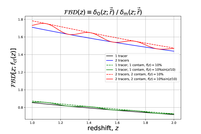
Figure 1: Example of the factor contaminant (contam), bias and growth of structure functional, $\mathcal{FBD}$, as a function of redshift, $z$, for $N=1$ order of correlation functional and different flavours of bias, and contaminant factors. The black line represents one tracer, with one bias, and no contaminant factor, while blue line represents two tracers with the same bias model and no contaminant factor. The green (red) dash line represents one (two) tracer(s) contaminated with a constant contaminant factor, $f(z)=10\%$. The same colors but with continuous line represent the same information but for a redshift evolved contaminant factor, $f(z)=10\%\sin(z/10)$. [See section 3.2.6]

3.2.6 An application on current concordance cosmology

We assume a simple cosmological model which describes part of the cosmological scales, i.e. the LSS and CMIB scales as follows. We consider the following fiducial concordance cosmology. We assume the speed of light, $c\simeq 3\times 10^{8}$ m/s, the dimensionless Hubble constant, $h=0.67$; the present baryon density ratio, $\Omega_{\rm b,0}=0.05$; the present matter density ratio, $\Omega_{\rm m,0}=0.32$; present dark energy density ratio, $\Omega_{\Lambda,0}=0.68$; the primordial power spectrum scalar amplitude, $A_{\rm s}=2.1\times 10^{-9}$; the spectral index, $n_{\rm s}=0.97$. We neglect the neutrino mass, $\sum_{i}m_{\nu_{i}}=0$ eV while the effective number of neutrinos is, $N_{\rm eff}=3.046$. We assume general relativity, by imposing that the growth rate has $\gamma=0.545$ [49, 50].

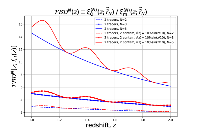
Figure 2: Example of the factor contaminant, bias and growth of structure functional, $\mathcal{FBD}$, as a function of redshift, $z$, for different $N$ order of correlation functional for two tracers assuming the same bias, and the same redshift evolved contaminant factor, $f(z)=10\%\sin(z/10)$. The blue (red) line represents two tracers with (without) contamination. The dash (dotted or continuous) line represents the order N=2 (3 or 5) of the correlation function. [See section 3.2.6]

Note that we can build an example by choosing a particular contaminant factor, bias and growth of structure model. We choose the following set as follows. We choose a simple model for the growth of structure

$$D(z)=\exp\left\{\int_{0}^{z}{\rm d}z^{\prime}\,\left[\frac{\Omega_{\rm m,0}\,(1+z^{\prime})^{3}}{H^{2}(z^{\prime})/H^{2}_{0}}\right]^{\gamma}\frac{-1}{1+z^{\prime}}\right\}\;.$$ (3.42)

We choose two functions which simulate some observations for the contaminant factor

$$f_{1}(z) =f_{0}$$ (3.43)

$$f_{2}(z) =f_{0}\sin(z/10)\;,$$ (3.44)

where $f_{0}$ is considered a free parameter with fiducial value $10\%$. We choose one popularly observed function for the deterministic bias model as,

$$b(z) =b_{0}\sqrt{1+z}\;,$$ (3.45)

where $b_{0}$ is a free parameter with fiducial value the unity.

In our application, we assume a targeted redshift range of interest, $1\leq z\leq 2$, and a contaminant redshift range of interest, $z_{\rm c}\in\left[2.0,2.5\right]$ for the first two examples, while for the last one we assume a contaminant redshift range which has smaller redshift values than the targeted one, i.e. $z_{\rm c}\in\left[0.2,0.8\right]$. In Figs. 1, 2 and 3, we present some quantitative examples of the factor contaminant, bias, and growth of structure functional as a function of redshift, $\mathcal{FBD}(z)$, as constructed by Eq. 3.29. For all cases in which we apply a sinusodial behaviour for the factor of contaminant, there is a sinusodial effect on the observed functional $\mathcal{FBD}(z)$, which is represented in all aforementioned figures.

From Fig. 1, we find as expected that

1. increasing (decreasing) number of tracers

2. increasing (decreasing) contaminant factor

results to an increasing (decreasing) functional, $\mathcal{FBD}(z)$. Doubling the number of tracers, existing in the same redshift region with the same bias model, results to a doubling of $\mathcal{FBD}(z)$. A $10\%$ increase of the contaminant factor results to a 2-1% ( 4-2.4% ) increase of the fuctional, $\mathcal{FBD}(z)$, for one (two) tracer in the targeted redshift range of interest.

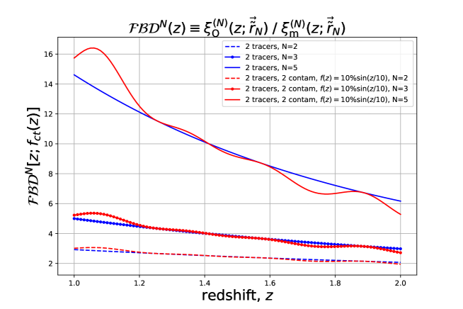
Figure 3: Similar to Fig. 2 with the difference that the contaminant redshift regions has smaller redshifts than the targeted one, i.e. the contaminant redshift region is $z_{\rm c}\in\left[0.2,0.8\right]$. [See section 3.2.6]

From Fig. 2, we additionally find that increasing (decreasing) order of correlation N, results to an increasing (decreasing) functional, $\mathcal{FBD}(z)$. For two tracers in the redshift range of interest, $1\leq z\leq 2$, an $10\%$ increase of the contaminant factor results to 20-10% ( 7-5% ) increase of the functional, $\mathcal{FBD}(z)$, for $N=5(2)$ order of correlation.

From Fig. 3, we find that for two tracers, for order of correlation $N=5(2)$, a $10\%$ increase of the contaminant factor from contaminants in lower redshift region, $z_{\rm c}\in[0.2,0.8]$, either produces up to a $18\%$ ($7\%$) increase of the $\mathcal{FBD}(z)$ functional from redshifts lower than $z_{\rm t}\lesssim 1.4$, or produces up to a $17\%$ ($6\%$) decrease of the $\mathcal{FBD}(z)$ functional at higher redshifts $z_{\rm t}\gtrsim 1.4$.

Overall, our results suggest that $10\%$ contamination from lower redshift produces up to a $18\%$ increase of the observed functional, $\mathcal{FBD}(z)$, at low redshifts $z_{\rm t}\lesssim 1.4$, while a $17\%$ decrease of $\mathcal{FBD}(z_{\rm t}\gtrsim 1.4)$, as opposed to $10\%$ contamination from higher redshifts, in which only up to a $20\%$ increase is produced, for $N=5$ order of correlation. This means that a special treatment is needed for these lower redshift contaminants.

3.3 Quantum scales (QS)

Quantum field theory has a long history with NPCF [29]. We know that the natural physical quantum systems are at least described by a Minkovskiy spacetime, in quantum scales. In this study, we expand this type of description in order to include a generalised Minkovskiy spacetime in NPCF of quantum mechanical systems. As in astronomical systems, we expect that the in quantum systems, there is also the need of a targeted quantum system and a contaminant one, which can be caused by elements which we would like not to target or observe. Therefore we can construct an NPCF in a such an object as we have achieved for astronomical scales. In quantum field theory an NPCF is described using a quantum field, $\phi(\vec{\tau x})\equiv\phi(\vec{\tau},\vec{x})$ using the equation

$$C_{N}\equiv C_{N}(\vec{\tau},\vec{x}_{1},\dots,\vec{x}_{N}) =\langle\phi(\vec{\tau},\vec{x}_{1})\dots\phi(\vec{\tau},\vec{x}_{D_{x}})\rangle_{\phi}$$ (3.46)

$$=\int_{\mathcal{M}^{\phi}}\mathcal{D}\phi\;\phi(\vec{\tau},\vec{x}_{1})\dots\phi(\vec{\tau},\vec{x}_{N})\;\exp\left\{{\frac{i}{\hbar}S[\vec{\tau x},\phi(\vec{\tau x})]}\right\}$$ (3.47)

where $S[\vec{\tau x},\phi]$ is the action which describes the physical system, $\hbar$ is the reduced Planck constant, $\mathcal{M}^{\phi}$ is the manifold of the field $\phi$, and we have used the completeness relation, i.e. $\int_{\mathcal{M}^{\phi}}\mathcal{D}\phi\;\exp\left\{{\frac{i}{\hbar}S[\vec{\tau x},\phi(\vec{\tau x})]}\right\}=1$. Note that in case which we would like to distinguish a targeted object category, in respect of several others which contaminate the targeted object category we can think the following, we can apply the description in section 2.4. Then for some targeted quantum field, $\phi_{t}(\vec{\tau x})$, some contaminated targeted quantum field, $\phi_{ct}(\vec{\tau x})$ and their respective decomposition functionals $D^{\phi}_{t}(\vec{\tau x})$, $D_{ct}^{\phi}(\vec{\tau x})\equiv D^{\phi}_{t}(\vec{\tau x})D_{ct}^{(F)\phi}(\vec{\tau x})$ and their universal quantum field functional $\phi_{\rm u}\equiv\phi_{u}(\vec{\tau_{i}x_{b}})$ we have

$$\phi(\vec{\tau x})=\phi_{\rm u}(\vec{\tau_{i}x}_{b})\sum_{t=1}^{N_{\rm t}}D^{\phi}_{t}(\vec{\tau},\vec{x})\left\{\left[1-\sum_{c=1}^{N_{{\rm c}t}}f_{ct}(\vec{\tau},\vec{x})\right]+\sum_{c=1}^{N_{{\rm c}t}}|\gamma_{ct}|^{D_{x}}(\vec{\tau})f_{ct}(\vec{\tau},\vec{x})D^{\rm(F)\phi}_{ct}(\vec{\tau},\vec{x})\right\}\;,$$ (3.48)

where $f_{ct}(\vec{\tau},\vec{x})$ is defined as the contaminant factor of targeted elementary particles which are contaminated by any natural contaminants appear at the level of their detections, such as non-targeted elementary particles, from other generalised spacetime regions, or composition of elementary particles, of even cosmic rays. Then, we can define the contaminated targeted functional as

$$\mathcal{C}^{\rm TF}(\vec{\tau x})=\sum_{t=1}^{N_{\rm t}}D^{\phi}_{t}(\vec{\tau},\vec{x})\left\{\left[1-\sum_{c=1}^{N_{{\rm c}t}}f_{ct}(\vec{\tau},\vec{x})\right]+\sum_{c=1}^{N_{{\rm c}t}}|\gamma_{ct}|^{D_{x}}(\vec{\tau})f_{ct}(\vec{\tau},\vec{x})D^{\rm(F)\phi}_{ct}(\vec{\tau},\vec{x})\right\}\;.$$ (3.49)

This means that $\phi(\vec{\tau x})=\phi_{\rm u}\;\mathcal{C}^{\rm TF}(\vec{\tau x})\;.$ In this case we have that the NPCF for a quantum field, $\phi$ is analysed as

$$C_{N}(\vec{\tau},\vec{x}_{1},\dots,\vec{x}_{N})=\int_{\mathcal{M}^{\phi}_{\rm u}}\mathcal{D}\phi_{\rm u}\left(\phi_{\rm u}\right)^{N}\int_{\mathcal{M}^{\mathcal{C}^{\rm TF}}}\mathcal{D}\mathcal{C}^{\rm TF}\;\;\mathcal{C}^{\rm TF}(\vec{\tau},\vec{x}_{1})\dots\mathcal{C}^{\rm TF}(\vec{\tau},\vec{x}_{N})\;e^{\left\{{\frac{i}{\hbar}S[\vec{\tau x},\phi_{\rm u},\mathcal{C}^{\rm TF}]}\right\}}$$ (3.50)

Note that the use of $C^{\rm FT}(\vec{\tau x})$ functional is the best way to specialise an observed NPCF for a generic quantum field. This formalism can be used in quantum field theory experiments, such as the LHC.

4 Conclusion

In this paper, we constructed a mathematical formalism for $(D_{\tau},D_{x})$-dimensional manifolds with $N$-correlators, i.e. the N-point correlation functional (NPCF) of $N_{t}$ types of objects with and without cross correlations and/or contaminants. In particular, we build this formalism using simple notions of mathematical physics, field theory, topology, algebra, statistics, N-correlators and Fourier transform. We discuss this formalism in the context of cosmological scales, i.e. from astronomical scales to quantum scales. We find that for the current interpretation of the astronomical scales, the problem of model selection can be reduced from a $(D_{\tau},D_{x})$-dimensional manifold, to a (redshift,spatial)-dimensional manifold, $\mathcal{M}^{(D_{z},D_{x})}$, using the observed functional form of the scale independent contaminant, bias and growth of structure as a function of redshift, formally written as $\mathcal{FBD}(\vec{\tau},\vec{x})\rightarrow\mathcal{FBD}(z)$, as well as the standard NPCF of the matter density field, their input functions and parameter dependences. Using current concordance cosmology, a quantitative analysis of a special configuration shows that there is up to a $20\%$ increase of the observed functional, $\mathcal{FBD}(z)$, for two possible matter tracers, in a targeted redshift region of $1\leq z_{\rm t}\leq 2$, with two possible contaminants, from higher redshifts, $2\leq z_{\rm c}\leq 2.5$, for $N\leq 5$ order of correlators. However, there is a dependence of the number of tracers and the redshift direction of these contaminants (lower or higher redshifts). This means that a special treatment is needed for these applications. We conclude that anything that affects the modelling and observation of the factor contaminant, bias and growth of structure functional, will affect also the model selection, and parameter inferences from current and future cosmological surveys and experiments. Furthermore, in quantum scales, we have found that this formalism corresponds to a specialisation of the NPCF for a generic quantum field used so far. In general, we conclude that this formalism can be used to any current and future cosmological survey and experiment, for model selection and parameter quantification inferences.

$\mathcal{O}.\mathcal{E}.\Delta$.

AKNOWLEDGEMENTS

PN would like to thank A.J.Hawken, S.Camera, A.Pourtsidou, B.Grannet, S.Avila, C. Uhlemann, F.Leclercq, Y.Wang, W.J.Percival, P. Schneider, A.Tilquin, P.L. Monaco, C. Scarlata, A.M.Dizgah, E.Sefussatti, G. E. Addison, and E.Castorina, for inspiring this project. We acknowledge open libraries support IPython [51], Matplotlib [52], NUMPY [53], SciPy 1.0 [54], IMINUIT [55], COSMOPIT [56, 57]. The FBDz code product of this analysis is publicly available.

Appendix A Statements & declarations

A.1 Funding

The authors declare that no funds, grants, or other support were received during the preparation of this manuscript.

A.2 Competing interests

The authors have no relevant financial or non-financial interests to disclose.

A.3 Author contributions

All authors contributed to the study conception and design. Material preparation, data collection and analysis were performed by Pierros Ntelis. The first draft of the manuscript was written by Pierros Ntelis and all authors commented on previous versions of the manuscript. All authors read and approved the final manuscript.

A.4 Data availability

Data sharing is not applicable to this article as no new data were created or analyzed in this study.

References

- Guth [1981] Guth, A. H. Inflationary universe: A possible solution to the horizon and flatness problems. Phys. Rev. D, 23:347–356, 1981.
- Linde [1982] Linde, A. D. A new inflationary universe scenario: A possible solution of the horizon, flatness, homogeneity, isotropy and primordial monopole problems. Physics Letters B, 108:389–393, 1982.
- Guth and Pi [1982] Guth, A. H. and S.-Y. Pi. Fluctuations in the new inflationary universe. Phys. Rev. Lett., 49:1110–1113, 1982.
- Starobinsky [1982] Starobinsky, A. A. Dynamics of phase transition in the new inflationary universe scenario and generation of perturbations. Physics Letters B, 117:175–178, 1982.
- Bardeen et al. [1983] Bardeen, J. M., P. J. Steinhardt, and M. S. Turner. Spontaneous creation of almost scale-free density perturbations in an inflationary universe. Phys. Rev. D, 28:679–693, 1983.
- Linde [1992a] Linde, A. Stochastic approach to tunneling and baby universe formation. Nuclear Physics B, 372:421–442, 1992a. arXiv:hep-th/hep-th/9110037.
- Linde [1992b] Linde, A. Strings, textures, inflation and spectrum bending. Physics Letters B, 284:215--222, 1992b. arXiv:hep-ph/hep-ph/9203214.
- Matarrese et al. [2000] Matarrese, S., L. Verde, and R. Jimenez. The Abundance of High-Redshift Objects as a Probe of Non-Gaussian Initial Conditions. Astrophysical Journal, 541:10--24, 2000. arXiv:astro-ph/astro-ph/0001366.
- Komatsu and Spergel [2001] Komatsu, E. and D. N. Spergel. Acoustic signatures in the primary microwave background bispectrum. Physical Review D, 63:063002, 2001. arXiv:astro-ph/astro-ph/0005036.
- Planck Collaboration et al. [2020a] Planck Collaboration, N. Aghanim, Y. Akrami, et al. Planck 2018 results. VI. Cosmological parameters. Astronomy and Astrophysics, 641:A6, 2020a. arXiv:astro-ph.CO/1807.06209.
- Hamaus et al. [2011] Hamaus, N., U. Seljak, and V. Desjacques. Optimal constraints on local primordial non-Gaussianity from the two-point statistics of large-scale structure. Physical Review D, 84:083509, 2011. arXiv:astro-ph.CO/1104.2321.
- Slosar et al. [2008] Slosar, A., C. Hirata, U. Seljak, et al. Constraints on local primordial non-Gaussianity from large scale structure. Journal of Cosmology and Astroparticle Physics, 2008:031, 2008. arXiv:astro-ph/0805.3580.
- Matarrese and Verde [2008] Matarrese, S. and L. Verde. The Effect of Primordial Non-Gaussianity on Halo Bias. Astrophysical Journal, Letters, 677:L77, 2008. arXiv:astro-ph/0801.4826.
- Dalal et al. [2008] Dalal, N., O. Doré, D. Huterer, et al. Imprints of primordial non-Gaussianities on large-scale structure: Scale-dependent bias and abundance of virialized objects. Physical Review D, 77:123514, 2008. arXiv:astro-ph/0710.4560.
- Castorina et al. [2019] Castorina, E., N. Hand, U. Seljak, et al. Redshift-weighted constraints on primordial non-Gaussianity from the clustering of the eBOSS DR14 quasars in Fourier space. Journal of Cosmology and Astroparticle Physics, 2019:010, 2019. arXiv:astro-ph.CO/1904.08859.
- Planck Collaboration et al. [2020b] Planck Collaboration, Y. Akrami, F. Arroja, et al. Planck 2018 results. IX. Constraints on primordial non-Gaussianity. Astronomy and Astrophysics, 641:A9, 2020b. arXiv:astro-ph.CO/1905.05697.
- Kirby et al. [2007] Kirby, E. N., P. Guhathakurta, S. M. Faber, et al. The DEEP2 Galaxy Redshift Survey: Redshift Identification of Single-Line Emission Galaxies. Astrophysical Journal, 660:62--71, 2007. arXiv:astro-ph/astro-ph/0701747.
- Pullen et al. [2016] Pullen, A. R., C. M. Hirata, O. Doré, et al. Interloper bias in future large-scale structure surveys. 2016. arXiv:astro-ph.CO/1507.05092.
- Wong et al. [2016] Wong, K., A. Pullen, and S. Ho. Filtering interlopers from galaxy surveys. arXiv e-prints, page arXiv:1606.08864, 2016. arXiv:astro-ph.IM/1606.08864.
- Addison et al. [2019] Addison, G. E., C. L. Bennett, D. Jeong, et al. The Impact of Line Misidentification on Cosmological Constraints from Euclid and Other Spectroscopic Galaxy Surveys. Astrophysical Journal, 879:15, 2019. arXiv:astro-ph.CO/1811.10668.
- Grasshorn Gebhardt et al. [2019] Grasshorn Gebhardt, H. S., D. Jeong, H. Awan, et al. Unbiased Cosmological Parameter Estimation from Emission-line Surveys with Interlopers. Astrophysical Journal, 876:32, 2019. arXiv:astro-ph.CO/1811.06982.
- Massara et al. [2020] Massara, E., S. Ho, C. M. Hirata, et al. Line confusion in spectroscopic surveys and its possible effects: Shifts in Baryon Acoustic Oscillations position. arXiv e-prints, page arXiv:2010.00047, 2020. arXiv:astro-ph.CO/2010.00047.
- Fonseca and Camera [2020] Fonseca, J. and S. Camera. High-redshift cosmology with oxygen lines from H surveys. Monthly Notices of the RAS, 495:1340--1348, 2020. arXiv:astro-ph.CO/2001.04473.
- Garrett-Roe and Hamm [2008] Garrett-Roe, S. and P. Hamm. Three-point frequency fluctuation correlation functions of the oh stretch in liquid water. The Journal of Chemical Physics, 128:104507, 2008. https://doi.org/10.1063/1.2883660.
- Berryman [1988] Berryman, J. G. Interpolating and integrating three-point correlation functions on a lattice. Journal of Computational Physics, 75:86--102, 1988.
- Dotsenko [1991] Dotsenko, V. Three-point correlation functions of the minimal conformal theories coupled to 2d gravity. Modern Physics Letters A, 06:3601--3612, 1991.
- Hwang et al. [1993] Hwang, K., B. Schmittmann, and R. K. P. Zia. Three-point correlation functions in uniformly and randomly driven diffusive systems. Phys. Rev. E, 48:800--809, 1993.
- Šanda and Mukamel [2005] Šanda, F. c. v. and S. Mukamel. Multipoint correlation functions for continuous-time random walk models of anomalous diffusion. Phys. Rev. E, 72:031108, 2005.
- Peskin and Schroeder [1995] Peskin, M. E. and D. V. Schroeder. An Introduction to Quantum Field Theory. Westview Press, 1995. Reading, USA: Addison-Wesley (1995) 842 p.
- Philcox et al. [2021] Philcox, O. H. E., Z. Slepian, J. Hou, et al. ENCORE: An {O}(N_g(2)) Estimator for Galaxy N-Point Correlation Functions. Monthly Notices of the RAS, 2021. arXiv:astro-ph.IM/2105.08722.
- Philcox and Slepian [2021] Philcox, O. H. E. and Z. Slepian. Efficient Computation of -point Correlation Functions in Dimensions. arXiv e-prints, page arXiv:2106.10278, 2021. arXiv:astro-ph.IM/2106.10278.
- Moore et al. [2001] Moore, A. W., A. J. Connolly, C. Genovese, et al. Fast Algorithms and Efficient Statistics: N-Point Correlation Functions. In Banday, A. J., S. Zaroubi, and M. Bartelmann, editors, Mining the Sky, page 71, 2001, arXiv:astro-ph/astro-ph/0012333.
- Ntelis [2020] Ntelis, P. Functors of actions. arXiv e-prints, page arXiv:2010.06707, 2020. arXiv:physics.gen-ph/2010.06707.
- Laureijs et al. [2011] Laureijs, R., J. Amiaux, S. Arduini, et al. Euclid Definition Study Report. arXiv e-prints, page arXiv:1110.3193, 2011. arXiv:astro-ph.CO/1110.3193.
- DESI Collaboration et al. [2016] DESI Collaboration et al. The DESI Experiment Part I: Science,Targeting, and Survey Design. arXiv e-prints, page arXiv:1611.00036, 2016. arXiv:astro-ph.IM/1611.00036.
- Rhodes et al. [2017] Rhodes, J., , et al. Scientific Synergy between LSST and Euclid. Astrophysical Journal, Supplement, 233:21, 2017. arXiv:astro-ph.IM/1710.08489.
- Abbott et al. [2016] Abbott, B. P. et al. Observation of gravitational waves from a binary black hole merger. Phys. Rev. Lett., 116:061102, 2016.
- Maggiore et al. [2020] Maggiore, M. et al. Science case for the Einstein telescope. Journal of Cosmology and Astroparticle Physics, 2020:050, 2020. arXiv:astro-ph.CO/1912.02622.
- Ntelis [2023] Ntelis, P. Generalised manifold-metric pairs. In preparation, 2023.
- Ntelis [2022] Ntelis, P. A probabilistic expanding Universe ! In preparation, 2022.
- Boone et al. [2021] Boone, K., , et al. The Twins Embedding of Type Ia Supernovae. II. Improving Cosmological Distance Estimates. Astrophysical Journal, 912:71, 2021. arXiv:astro-ph.CO/2105.02204.
- Ma and Bertschinger [1995] Ma, C.-P. and E. Bertschinger. Cosmological Perturbation Theory in the Synchronous and Conformal Newtonian Gauges. Astrophysical Journal, 455:7, 1995. arXiv:astro-ph/astro-ph/9506072.
- Blanton et al. [2017] Blanton, M. R. et al. Sloan Digital Sky Survey IV: Mapping the Milky Way, Nearby Galaxies, and the Distant Universe. Astronomical Journal, 154:28, 2017. arXiv:astro-ph.GA/1703.00052.
- G. Karaçaylı et al. [2021] G. Karaçaylı, N., N. Padmanabhan, Font-Ribera, et al. Optimal 1D Ly Forest Power Spectrum Estimation -- II. KODIAQ, SQUAD & XQ-100. arXiv e-prints, page arXiv:2108.10870, 2021. arXiv:astro-ph.CO/2108.10870.
- Baker and Harrison [2020] Baker, T. and I. Harrison. Constraining Scalar-Tensor Modified Gravity with Gravitational Waves and Large Scale Structure Surveys. arXiv e-prints, page arXiv:2007.13791, 2020. arXiv:astro-ph.CO/2007.13791.
- Lewis and Challinor [2006] Lewis, A. and A. Challinor. Weak gravitational lensing of the CMB. Physics Reports, 429:1--65, 2006. arXiv:astro-ph/astro-ph/0601594.
- Sherwin and Schmittfull [2015] Sherwin, B. D. and M. Schmittfull. Delensing the CMB with the CIB. Physical Review D, 92:043005, 2015. arXiv:astro-ph.CO/1502.05356.
- Ilić et al. [2021] Ilić, S., N. Aghanim, C. Baccigalupi, et al. preparation: XV. Forecasting cosmological constraints for the and CMB joint analysis. arXiv e-prints, page arXiv:2106.08346, 2021. arXiv:astro-ph.CO/2106.08346.
- Lahav et al. [1991] Lahav, O., P. B. Lilje, J. R. Primack, et al. Dynamical effects of the cosmological constant. Monthly Notices of the RAS, 251:128--136, 1991.
- Linder and Cahn [2007] Linder, E. V. and R. N. Cahn. Parameterized beyond-einstein growth. Astroparticle Physics, 28:481--488, 2007. arXiv:astro-ph/0701317v2.
- Perez and Granger [2007] Perez, F. and B. E. Granger. Ipython: A system for interactive scientific computing. Computing in Science Engineering, 9:21--29, 2007.
- Hunter [2007] Hunter, J. D. Matplotlib: A 2d graphics environment. Computing in Science & Engineering, 9:90--95, 2007.
- Walt et al. [2011] Walt, S. v. d., S. C. Colbert, and G. Varoquaux. The numpy array: A structure for efficient numerical computation. Computing in Science and Engg., 13:22--30, 2011.
- Virtanen et al. [2019] Virtanen, P., R. Gommers, T. E. Oliphant, et al. SciPy 1.0--Fundamental Algorithms for Scientific Computing in Python. arXiv e-prints, page arXiv:1907.10121, 2019. arXiv:cs.MS/1907.10121.
- James and Roos [1975] James, F. and M. Roos. Minuit: A System for Function Minimization and Analysis of the Parameter Errors and Correlations. Comput. Phys. Commun., 10:343--367, 1975.
- Ntelis et al. [2017] Ntelis, P., J.-C. Hamilton, J.-M. Le Goff, et al. Exploring cosmic homogeneity with the BOSS DR12 galaxy sample. Journal of Cosmology and Astroparticle Physics, 2017:019, 2017. arXiv:astro-ph.CO/1702.02159.
- Ntelis et al. [2018] Ntelis, P., A. Ealet, S. Escoffier, et al. The scale of cosmic homogeneity as a standard ruler. Journal of Cosmology and Astroparticle Physics, 2018:014, 2018. arXiv:astro-ph.CO/1810.09362.